Kinematics and Dynamics of kiloparsec-scale Jets in Radio Galaxies with SKA

Abstract:

We explore the use of SKA to deduce the physical parameters of kiloparsec-scale jet flows in radio galaxies. Jets in Active Galactic Nuclei are relativistic where they are first formed, but their speeds and compositions change as they propagate. It has long been known that kiloparsec-scale jets in radio galaxies can be divided into two flavours: strong (found in powerful sources, narrow and terminating in compact hot-spots) and weak (found in low-luminosity sources, geometrically flaring, unable to form hot-spots and terminating in diffuse lobes or tails). We have developed methods to model AGN jets as intrinsically symmetrical, relativistic flows by fitting to deep, well-resolved radio images in Stokes $I$, $Q$ and $U$. This has yielded a wealth of information about the brightest few weak-flavour jets. Our first key objective is to observe large samples of weak and transition jets at 0.1 – 0.5 arcsec resolution with SKA1-MID. This would allow us to see how jet propagation depends on power and environment and to quantify the energy and momentum input into the IGM. We will require typical noise levels of 1$\mu$Jy/beam, and may be able to exploit survey imaging in some cases. Our second, more challenging, application is to determine the velocity fields in strong-flavour jets. Do they have very fast ($\Gamma\approx 5-10$) spines? Is there evidence for magnetic confinement by a toroidal field? What are their energy fluxes? This is a major imaging challenge for SKA2: we need resolution better than 0.05 arcsec, ideally in the 1 – 10 GHz frequency range, with rms noise levels $\approx$10 nJy/beam and extremely high dynamic range, imaging fidelity and polarization purity.

1 Introduction

Jets from active galactic nuclei (AGN) are important in many areas of astrophysics: they extract energy from supermassive black holes, produce the most energetic photons (and perhaps cosmic rays) we observe, act as conveyors of ultrarelativistic particles and magnetic fields from the parsec-scale environments of AGN to the multi-kiloparsec scales of extended radio galaxies and quasars, and supply copious amounts of energy to their surroundings, thereby preventing cooling and profoundly affecting the evolution of massive galaxies and clusters.

An overview of the study of AGN jets with SKA is given by Agudo et al., (2015). This paper covers one aspect – the physics of jets on kpc scales – in more detail, emphasising a number of key topics (cf. Blandford, 2008), as follows.

1. What are the velocity fields? Why do some jets expand rapidly, increase in brightness and decelerate while others remain fast and collimated? How does this relate to the origin of the Fanaroff-Riley classes (Fanaroff & Riley, 1974)?

2. How does jet composition change with distance from the AGN? What are the typical mass fluxes and entrainment rates?

3. What is the magnetic-field topology on kpc scales – ordered or disordered?

4. How is jet propagation determined by the external environment (density, pressure, temperature, magnetization)?

5. How are jets confined: by external gas pressure, magnetic fields, some other mechanism or not at all?

6. Where and by what process are relativistic particles accelerated?

7. What are the jet energy and momentum fluxes?

8. What effects do the jets have on their surrounding IGM/ICM? Do they lead to shocks and heating? What effect do they have on external magnetic fields and hence on thermal transport?

It has long been known that AGN radio jets divide into strong and weak ‘flavours’ (Bridle, 1984). Strong-flavour jets are usually one-sided ($>$4:1) and well-collimated over their whole lengths and often terminate in compact hot spots. Weak-flavour jets are initially asymmetric, but tend to symmetrize far from the nucleus. They also ‘flare’ with increasing distance from the AGN in two distinct senses: geometrically (a significant increase in apparent spreading rate) and in brightness (an increase in apparent intensity, often following an initial ‘gap’, or extended region in which the radio emission is weak or undetectable). The qualitative picture is that both jet flavours are initially relativistic, but weak-flavour jets decelerate to subrelativistic speeds on kpc scales, while strong-flavour jets remain highly relativistic until they reach the outer parts of the sources.

Thus far, we have derived quantitative models only for a small number of weak-flavour jets using deep VLA observations. Strong-flavour jets are harder to study as they are narrower than weak-flavour jets (thus harder to resolve) and their counter-jets are faint and difficult to isolate from surrounding lobe emission. After outlining the modelling methods and associated imaging requirements (Section 2), we therefore consider in turn the use of SKA1-MID to observe large samples of weak-flavour jets (Section 3) and SKA2 to model strong-flavour jets for the first time with our methods (Section 4).

2 Measuring the flow parameters of jets

Although numerical (GRMHD) simulations of jet formation have made considerable progress recently (e.g. McKinney et al., 2013), the problem of simulating the propagation of a very light, relativistic, magnetized jet in three dimensions is computationally prohibitive, with poorly known initial conditions: no simulation can yet hope to follow a jet all the way from its formation on scales comparable with the gravitational radius of the central black hole to the kiloparsec scales which SKA can best resolve. A more empirical approach to estimation of jet flow parameters is therefore needed.

One powerful method is based on the realization that kpc-scale jets are both significantly relativistic and intrinsically symmetrical, in the specific sense that apparent asymmetries due to relativistic aberration are much larger than any intrinsic asymmetries. Jets emit (often highly) polarized synchrotron radiation. With the assumptions that the flows are (on average) axisymmetric, intrinsically symmetrical and stationary, the observed brightness distributions in Stokes $I$, $Q$ and $U$ can be modelled to fit for geometry, velocity field, intrinsic emissivity variation and three-dimensional magnetic field configuration. The method was first described in Laing & Bridle, 2002a ; a comprehensive overview is given by Laing & Bridle, (2014). The key to the method is to determine the velocity and inclination angle independently by comparing emission from the main and counter-jets in both total intensity and linear polarization. The observed polarizations in the approaching and receding jets are not the same because they are effectively observed at different angles to the line of sight in the rest frame, $\theta^{\prime}$. For antiparallel jets at angle $\theta$ to the line of sight in the observed frame,

$$\sin\theta^{\prime}_{\rm j} = [\Gamma(1-\beta\cos\theta)]^{-1}\sin\theta$$

$$\sin\theta^{\prime}_{\rm cj} = [\Gamma(1+\beta\cos\theta)]^{-1}\sin\theta$$

where subscripts j and cj refer to the approaching and receding jets, $\beta$ is the flow velocity in units of $c$ and $\Gamma$ is the bulk Lorentz factor. $\beta$ and $\theta$ cannot be determined independently from images of total intensity alone: the use of linear polarization is crucial.

This method has proved to be very successful in modelling the jet flows in bright, nearby (FR I) radio galaxies, as we describe in Section 3. Given the derived velocity fields (and the assumption of pressure equilibrium with the surroundings on large scales), we can also use the laws of conservation of mass, momentum and energy to estimate the energy and mass fluxes and the run of entrainment rate along the jets (Laing & Bridle, 2002b ). The magnetic-field topology is not completely determined, however. The models show that longitudinal and toroidal components dominate (at small and large distances, respectively). The observed symmetry of the transverse profiles of $I$ and $Q$ tells us that the field structure is not a simple ‘grand design’ helix on these scales (Laing et al., 2003), but leaves open the question of whether the toroidal component is vector-ordered. If it is, there should be systematic gradients in Faraday rotation across the jets (we know that thermal electrons must be entrained even if they are not present near the AGN). Such searches have so far been frustrated by large fluctuations in foreground Faraday rotation.

The observational requirements for this technique are images of both jets with good fidelity, at least 5 and preferably $>$10 beams across their widths and noise levels low enough to detect 10% polarization at $4\sigma$ everywhere. It must also be possible to correct the effects of Faraday rotation (and depolarization) to high accuracy.

These methods have so far managed to provide answers to many of the questions posed in Section 1, but only for a small number of carefully selected sources. We have been restricted to jets which are bright and easily resolved. Thus we sample a limited (intermediate) range of luminosity, and can only model jets with large opening angles. We know very little about more powerful, highly-collimated jets, intrinsically weak sources or the systematic dependences of jet physics on power and environment. To do better, we need much large samples of low-luminosity sources (high sensitivity at moderate resolution) and an instrument capable of much higher resolution and very high sensitivity for the powerful sources. We explore these applications in the following two sections.

3 Decelerating jets: SKA1-MID

3.1 Current results

Our current results on decelerating, FR I jets are summarised in Laing & Bridle, (2014), and an example is shown in Fig. 1. All of the jets first increase in opening angle and then recollimate to form conical flows at a fiducial distance $r_{0}$ (the flaring region) in the range 2 – 35 kpc from the AGN. At $\approx$0.1$r_{0}$, the jets brighten abruptly at the onset of a high-emissivity region and we find an outflow speed of $\approx$0.8$c$, with a uniform transverse profile. Jet deceleration first becomes detectable at $\approx$0.2$r_{0}$ and the outflow often becomes slower at its edges than it is on-axis. Deceleration continues until $\approx$0.6$r_{0}$, after which the outflow speed is usually constant. The dominant magnetic-field component is longitudinal close to the AGN and toroidal after recollimation, but the field evolution is initially much slower than predicted by flux-freezing. In the flaring region, acceleration of ultrarelativistic particles is required to counterbalance the effects of adiabatic losses and account for observed X-ray synchrotron emission, but the brightness evolution of the outer jets is consistent with adiabatic losses alone. These results are best interpreted as effects of the interaction between the jets and their surroundings. The initial increase in brightness occurs in a rapidly falling external pressure gradient in a hot, dense, kpc-scale corona around the AGN. We interpret the high-emissivity region as the base of a transonic ‘spine’ and suggest that a subsonic shear layer starts to penetrate the flow there. Most of the resulting entrainment must occur before the jets start to recollimate.

Figure 1: Observations and models of the nearby radio galaxy NGC 315 (Laing & Bridle, 2014). (a) Vectors with magnitudes proportional to the degree of polarization, $p$, and directions along the apparent magnetic field superposed on a false-colour plot of total intensity. (b) Model fit corresponding to (a). (c) The derived velocity field, in units of $c$.

3.2 SKA1-MID observations

While the basic process of jet deceleration in twin-jet sources has become clearer, there are still many unanswered questions. Almost all of the sources we have modelled so far have luminosities close to $P\approx 10^{24.5}$ WHz^-1 at 1.4 GHz. The next set of questions includes the following.

1. How does the characteristic recollimation scale $r_{0}$ vary with luminosity (jet power) and external pressure? Can we develop a way of predicting a priori which jets will decelerate and the form of their outer structures?

2. What are the distributions of energy and mass flux? How do these depend on black hole mass, accretion rate and ISM/IGM properties? Do they correlate with estimates from the size and pressure of jet-blown ‘cavities’ in the IGM/ICM? Can we infer the energy and momentum input integrated over the source population for comparison with galaxy formation models?

3. What causes jet emission to ‘turn on’ at the flaring point, $\approx 0.1r_{0}$?

4. How important is stellar mass input in decelerating the weakest jets (it can be differentiated from boundary-layer entrainment because no slow boundary layer is formed)?

5. Can we decide unequivocally whether the toroidal field component is vector ordered and, if so, does it contribute to jet collimation on kpc scales? [To do this, we will need to measure Faraday rotation for a sample of sources selected to have low foreground contamination.]

6. How important are intrinsic and environmental asymmetries? This cannot be assessed for an individual object, but relativistic and environmental asymmetries are expected to be uncorrelated, so we can separate their effects statistically for a sufficiently large sample.

In order to answer these questions with any statistical significance, we will need to increase the number of modelled sources from 10 to at least a few hundred and to identify sub-samples with different luminosities and environments. Our long VLA observations typically reach rms noise levels between 5 and 10$\mu$Jy/beam at angular resolutions between 0.25 and 2.5 arcsec (The upgraded Karl G. Jansky VLA is allowing us to go up to a factor of 5 deeper, but only with long multi-configuration observations in special cases). For an integral source count $N(>S)\propto S^{-1.5}$ (appropriate for these nearby sources), we would need to increase the sensitivity by a factor of 10 from the flux densities alone (i.e. an rms noise level of $0.5-1.0\mu$Jy/beam). Detailed trade-offs depend on source brightness, size and environment. For example: the need to measure low Faraday rotations argues for lower frequencies, but we cannot tolerate a significant variation of rotation across the observing beam; there are systematic variations of jet size (and therefore required resolution) with luminosity, and so on. Band 3 is therefore preferred for the measurement of low Faraday depths; Band 5 for jet modelling. These observations would also probe the magnetoionic environments of the radio galaxies in great detail (Laing et al., 2008; Guidetti et al., 2011).

An initial estimate is that we would need $\approx$300 observations (mostly pointed, but perhaps also obtained from surveys) with high image fidelity, resolution $\approx$0.25  arcsec and rms noise level   $\buildrel<\over{\sim}$  1 $\mu$Jy/beam in SKA1-MID, Band 5. For the combined SKA1-MID array (Dewdney et al., 2013, Table 9) and allowing for a factor of 2 increase in noise from weighting (Braun, 2013), this would give an average of   $\buildrel>\over{\sim}$  50 min on-source time per observation, or   $\buildrel>\over{\sim}$  240 hr in total. The observations would still be feasible in an Early Science phase, but longer integrations (by factors   $\buildrel>\over{\sim}$  4) or correspondingly smaller sample sizes would be required.

4 Fast, powerful jets: SKA2

The strong-flavour jets found in powerful radio galaxies and quasars, particularly those associated with FR II sources, are far harder to study, as they are narrow and (in the case of counter-jets) also very faint (e.g. Fig. 2).

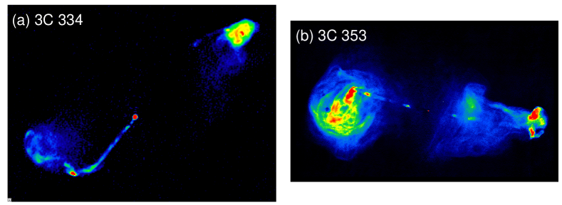
Figure 2: VLA images of (a) the powerful quasar 3C 334 (Bridle et al., 1994) and (b) the radio galaxy 3C 353 (Swain et al., 1998). Note the very narrow strong-flavour jets. 3C 334 is thought to be at $\ {\raise-2.15277pt\hbox{$\buildrel<\over{\sim}$}}\ 40^{\circ}$ to the line of sight and shows a pronounced jet/counter-jet asymmetry (the counter-jet is only visible at large distances from the AGN). In contrast, 3C 353 is close to the plane of the sky and both jets are visible, but its asymmetries are dominated by the environment.

We aim to distinguish between two hypotheses: (a) strong jets are only mildly relativistic ($\beta\approx 0.5-0.7$; $\Gamma\approx 1.2-1.4$) as inferred naively from the statistics of their integrated sidedness ratios (Wardle & Aaron, 1997; Mullin & Hardcastle, 2009) or (b) they have a two-component velocity structure, with a much faster ($\beta>0.95$) spine surrounded by a slower shear layer that dominates the emission except in very end-on cases. Case (b) has long been suspected (Bridle et al., 1994), but never proved: arguments in favour include the following.

1. High pattern speeds are inferred from VLBI proper-motion measurements for pc-scale jets in flat-spectrum quasars (the end-on counterparts of sources like 3C 334; Lister et al., 2013). If these are representative of the bulk motion, then flow Lorentz factors up to $\Gamma\approx 40$ are required. Deceleration of such powerful jets to mildly relativistic speeds on kpc scales cannot occur without disruption.

2. If the X-rays observed in the extended jets associated with core-dominated sources are generated by inverse Compton scattering of cosmic microwave background photons by relativistic electrons in the jet, then the bulk Lorentz factors must be large ($\Gamma\ {\raise-2.15277pt\hbox{$\buildrel>\over{\sim}$}}\ 10$) and the jets must be close to the line of sight (Tavecchio et al., 2000; Celotti et al., 2001). Note, however, that there are arguments against this interpretation of the X-ray emission, at least in some sources (Hardcastle, 2006; Meyer & Georganopoulos, 2013).

3. The jet/counter-jet ratio and observations of apparent superluminal speeds in the jet of M 87 both indicate $\Gamma\ {\raise-2.15277pt\hbox{$\buildrel>\over{\sim}$}}\ 6$ over at least part of its length (Asada et al., 2014).

There are a number of transition cases between weak and strong-flavour jets which do not appear to decelerate significantly but which have counter-jets that can now be imaged with the VLA. The best example is NGC 6251 (Fig 3), for which observations are under way.

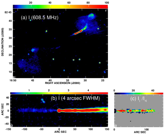
Figure 3: Images of NGC 6251. (a) Overall structure (WSRT, 609 MHz, from Mack et al., 1997). (b) Rotated image of the jets at 1665 MHz, 4 arcsec FWHM from archival VLA data. (c) Sidedness ratio $R=I_{\rm j}/I_{\rm cj}$, derived from (b) and blanked (grey) where $I<3\sigma$ in either jet. The jets in this source represent a transition between weak and strong flavours: they flare, but still maintain a large side-to-side ratio. The sidedness ratio image in panel (c) strongly suggests a substantial velocity gradient across the jets.

Modelling of true strong-flavour jets such as those found in luminous quasars is a far more challenging prospect, even for SKA2. Counter-jets can currently only be imaged with something approaching adequate s/n in sources such as 3C 353 (Fig. 2, Swain et al., 1998) which are very close to the plane of the sky (in which case our modelling technique does not work). We really need to image both jets in powerful sources which are reasonably inclined. As an example, if the straight part of the counter-jet in 3C 334 (Fig. 2) has $I\approx 10\mu$Jy/beam at 5 GHz with a beam of 0.35 arcsec (just below the current limit) and a width of 0.2 – 0.6 arcsec, we would need a resolution of $\approx$0.05 arcsec, and an rms noise level of $\ {\raise-2.15277pt\hbox{$\buildrel<\over{\sim}$}}\ 10$ nJy to be able to image and model the counter-jet in linear polarization. In turn, this requires a dynamic range of $\ {\raise-2.15277pt\hbox{$\buildrel>\over{\sim}$}}\ 10^{7}:1$ (peak:rms). Both requirements could be relaxed if adequate resolution could be obtained at a lower frequency.

5 Summary

We have outlined some of the ways in which SKA could contribute to the study of large-scale jets in radio galaxies. Extension of current work on low and intermediate luminosity sources to large samples is feasible for SKA1-MID. The case of powerful jets is an interesting challenge for SKA2.

References

- Agudo et al., (2015) Agudo, I., Böttcher, M., Falcke, H., et al. 2015, “Relativistic Jets”, in proceedings of “Advancing Astrophysics with the Square Kilometre Array”, PoS(AASKA14)093
- Asada et al., (2014) Asada K., Nakamura M., Do, A., Nagai H., & Inoue, M. 2014, ApJ, 781, L2
- Blandford, (2008) Blandford R. D. 2008, in Extragalactic Jets: Theory and Observation from Radio to Gamma Ray, ASP Conference Series, 386, 3
- Braun, (2013) Braun, R., “SKA1 Imaging Science Performance”, Document number SKA-TEL-SKO-DD-XXX Revision A Draft 2
- Bridle, (1984) Bridle A. H. 1984, AJ, 89, 979
- Bridle et al., (1994) Bridle A. H., Hough D. H., Lonsdale C. J. Burns J. O., & Laing R. A. 1994, AJ, 108, 766
- Celotti et al., (2001) Celotti A., Ghisellini G., & Chiaberge M. 2001, MNRAS, 321, L1
- Dewdney et al., (2013) Dewdney, P., Turner, W., Millenaar, R., McCool, R., Lazio, J., Cornwell, T. 2013, “SKA1 System Baseline Design”, Document number SKA-TEL-SKO-DD-001 Revision 1
- Fanaroff & Riley, (1974) Fanaroff B. L., & Riley J. M. 1974, MNRAS, 167, 31p
- Guidetti et al., (2011) Guidetti D., Laing R. A., Bridle A. H., Parma P., & Gregorini L. 2011, MNRAS, 413, 2525
- Hardcastle, (2006) Hardcastle M. J. 2006, MNRAS, 366, 1465
- (12) Laing R. A., & Bridle A. H. 2002a, MNRAS, 336, 328
- (13) Laing R. A., & Bridle A. H. 2002b, MNRAS, 336, 1161
- Laing & Bridle, (2014) Laing R. A., & Bridle A. H. 2014, MNRAS, 437, 3405
- Laing et al., (2008) Laing R. A., Bridle A. H., Parma P., & Murgia M. 2008, MNRAS, 391, 521
- Laing et al., (2003) Laing R. A., Canvin J. R., & Bridle A. H. 2003, AN, 327, 523
- Lister et al., (2013) Lister M. L., Aller M. F., Aller H. D., et al. 2013, AJ, 146, 120
- Mack et al., (1997) Mack, K.-H., Klein, U., O’Dea, C. P., Willis, A. G. 1997, A&AS, 123, 423
- McKinney et al., (2013) McKinney J. C., Tchekhovskoy A., & Blandford R. D. 2013, Science, 339, 49
- Meyer & Georganopoulos, (2013) Meyer, E. T., & Georganopoulos M. 2014, ApJ, 780, L27
- Mullin & Hardcastle, (2009) Mullin L. M., & Hardcastle M. J. 2009, MNRAS, 398, 1989
- Tavecchio et al., (2000) Tavecchio F., Maraschi L., Sambruna R. M., & Urry C. M. 2000, ApJ, 544, L23
- Swain et al., (1998) Swain M.R., Bridle A.H., & Baum, S.A., 1998 ApJ, 507, L29
- Wardle & Aaron, (1997) Wardle J.F.C., & Aaron S.E., 1997 MNRAS, 286, 425