Regularization dependence on phase diagram in Nambu–Jona-Lasinio model
Abstract
We study the regularization dependence on meson properties and the phase diagram of quark matter by using the two flavor Nambu–Jona-Lasinio model. We find that the meson properties and the phase structure do not show drastically difference depending the regularization procedures. We also find that the location or the existence of the critical end point highly depends on the regularization methods and the model parameters. Then we think that regularization and parameters are carefully considered when one investigates the QCD critical end point in the effective model studies.
I INTRODUCTION
The phase structure of quark matter on finite temperature and density has actively been studied for decades Fukushima:2010bq . Under usual condition, meaning low temperature and density, quarks are confined inside hadrons and they never be able to observed as a single particle. On the other hand, due to the nature of the asymptotic freedom Gross:1973id , quarks and gluons can be free from the confinement at high temperature and density, because the coupling strength becomes weak at high energy. It is, therefore, expected that quark matter undergoes the confined/deconfined phase transition at some temperature and density. This is important subject both in theoretical and experimental studies since it crucially relates to the quark matter properties at relativistically high energy collisions and extremely dense stellar objects such as neutron stars.
The first principle for quarks and gluons is Quantum Chromodynamics (QCD) which is a non-Abelian gauge field theory for fermions. Our goals is to evaluate the phase structure based on this first principle QCD, however, it is difficult to extract theoretical predictions due to the nature of complicated strongly interacting system. One of the most reliable approaches is to use the discretised version of QCD called the Lattice QCD (LQCD) in which theoretical calculation is performed on the discrete spacetime Wilson:1974sk . Although the LQCD works well at finite temperature for small chemical potential , there is the technical difficulty called the “sign problem” when one tries to investigate the system at intermediate chemical potential. There effective models maybe nicely adopted because some models can consistently treat the system at finite temperature and chemical potential.
For the sake of evaluating the phase structure of quark matter at finite temperature and chemical potential, we will employ the Nambu–Jona-Lasinio (NJL) model NJL which is the most frequently used one in this context (there are a lot of nice review papers on the model, see, e.g. Vogl:1991qt ; Klevansky:1992qe ; Hatsuda:1994pi ; Buballa:2005rept ; Huang:2004ik .) The model is constructed by incorporating the four point quark interaction into the model Lagrangian, so it is not renormalizable due to this higher dimensional operator. Therefore, the physical predictions of the model inevitably depend on the regularization procedure and the model parameters chosen. The resulting phase diagram on the plane is as well affected by the parameters and regularization prescriptions. So it is an important issue to study whether the phase structure obtained in one regularization method is consistent with the ones from different regularization methods.
In this paper, we are going to study the phase structure of quark matter in the NJL model with various regularization ways, which are three dimensional (D) momentum cutoff, four dimensional (D) momentum cutoff, Pauli-Villars (PV) regularization, proper-time (PT) regularization, and the dimensional regularization (DR). The D cutoff scheme is the most popular method in this model and a lot of works have been done in this way. The D cutoff method preserves the Lorentz symmetry in which space and time are treated on equal footing. The Pauli-Villars regularization is based on the subtraction of the amplitude considering the virtually heavy particle to suppress the unphysical high energy contribution coming from loop integrals Pauli:1949zm ; Itzykson1980 ; Cheng1984 . The proper-time regularization makes integrals finite through the exponentially dumping factor Schwinger:1951nm ; Itzykson1980 . The dimensional regularization analytically continues the spacetime dimension in the loop integrals to a non-integer value, then try to obtain finite contribution from the integrals 'tHooft:1972fi . Beside from the frequently used D cutoff way, there have been a lot of works by using the D Klevansky:1992qe ; Hatsuda:1994pi , PV Klevansky:1992qe ; Kahana:1992jm ; Osipov:2004bj ; Moreira:2010bx , PT Klevansky:1992qe ; Suganuma:1990nn ; Klimenko:1990rh ; Klimenko:1991he ; Gusynin:1994re ; Inagaki:1997nv ; Inagaki:2003yi ; Inagaki:2004ih ; Inagaki:2003ac ; Cui:2014hya , and DR Krewald:1991tz ; jafarov:2004 ; jafarov:2006 ; inagaki:2008 ; Inagaki:2011uj ; Inagaki:2012re . The physical consequences depend on the regularization fujihara:2009 .
This paper is organized as follows; Section II introduces the model Lagrangian, and show the model treatment on the meson properties and the explicit formalism at finite temperature and chemical potential. In Sec. III, we present various regularization procedures, D, D, PV, PT and DR prescriptions with explicit equations. We then perform the parameter fitting in Sec. IV. In Sec. V, the numerical results of the meson properties are shown. We then draw the phase diagrams with several parameter sets using various regularization methods in Sec. VI. We also study the phase diagram with the parameters fixed under the condition with the same constituent quark mass in Sec. VII. In Sec. VIII, we give the discussions on the obtained results. Finally, we write the concluding remarks in Sec. IX. Several detailed calculations are shown in Appendix.
II Two flavor NJL model
In this paper we consider two light quarks with equal mass. The model has flavor symmetry at the massless limit, .
II.1 The Lagrangian and gap equation
The Lagrangian of the two flavor NJL model is given by
| (1) |
where is the diagonal mass matrix and is the effective coupling strength of the four point interaction. We set in this paper. The application of the mean-field approximation
| (2) |
leads the following mean-field Lagrangian
| (3) |
with the constituent mass . The flavor symmetry is broken down, , by non-vanishing current quark mass, , and dynamically generated . Thanks to the simple form of the Lagrangian, one can easily evaluate the effective potential, where is the partition function
| (4) |
and is the volume of the system. After some algebra, we see
| (5) |
The detailed derivation of the effective potential is presented in Huang:2004ik .
The gap equation is obtained through the extreme condition of the potential with respect to , namely,
| (6) |
This condition leads the following gap equation
| (7) |
with the number of flavors and
| (8) |
where trace takes the spinor and color indices. This is the key equation in the model because it determines the values of the chiral condensate and the constituent quark mass .
II.2 Meson properties
The properties of the pion and sigma meson can be studied based on the model with the determined chiral condensate. The interacting Lagrangian of the pion and quarks is written by
| (9) |
where are matrices in the flavor space and represent the pion fields. The explicit expression is , with and where are the Pauli matrices.
By applying the random phase approximation, we can write the pion propagator as the summation of the geometrical series of the one-loop diagram, which gives
| (10) |
where is the following quark loop contribution
| (11) |
with the quark propagator
| (12) |
The explicit derivation of Eq. (10) is discussed in the review paper Klevansky:1992qe . The pion mass is calculated at the pole position of the propagator, so the condition reads
| (13) |
It should be noted that the residue at the pole coincides with the square of the coupling strength so we have the relation
| (14) |
In the similar manner, the sigma meson mass is evaluated at the pole of the propagator,
| (15) |
with
| (16) |
Therefore the condition which determines the sigma meson mass becomes
| (17) |
The pion decay constant is calculated from the following equation
| (18) |
The explicit form becomes
| (19) |
II.3 Explicit formalism at finite temperature
Since our purpose is to study the phase structure on temperature and chemical potential , we need to extend the equations to finite temperature. According to the imaginary time formalism, the integral region of the temporal component becomes finite due to the periodic or anti-periodic condition of fields as
| (20) |
where is imaginary time and is the inverse temperature . Consequently, continuous integral in the temporal direction is replaced by the following discrete summation,
| (21) |
where or depending on the statistical property of field, i.e., for bosons or fermions, and the chemical potential seen in Eq. (20) appears in the way . In this paper, we only treat fermionic quark loop contributions then is always the case.
With the help of the formalism Eq.(21), we see that the gap equation at finite temperature becomes
| (22) | |||
| (23) | |||
| (24) |
where is the number of colors, , and . It is important to note that the contributions can be expressed by the summation of the independent part () and dependent part (). This characteristic is general if one takes the infinite number of the frequency summation in finite temperature field theory and crucial when we apply the regularization procedures to the appearing integrals.
Since the gap equation is derived by differentiating the effective potential with respect to , then the effective potential can be obtained by integrating the gap equation (see, for example, Inagaki:1995 ),
| (25) |
where we have dropped the suffix in and just written for notational simplicity. Thereafter the effective potential at finite temperature is evaluated as
| (26) | |||
| (27) | |||
| (28) |
It is important to note that, if we apply some regularizations, the results between the direct calculation from Eq. (5) and the one after integrating the gap equation may become different, because regularization essentially means the subtraction and there are several ways of subtractions. Therefore, in this paper, we persistently use the latter way shown in Eq. (25) so that the model treatment becomes consistent. It should be noticed that the finite temperature correction, , contains no divergent integral. A finite result can be obtained for the finite temperature correction without applying any regularizations.
Next, we carry on the integral in the meson properties; the one loop contribution can be written as
| (29) |
with
| (30) |
Since is already evaluated above, the remaining task is to calculate , and it becomes
| (31) | |||
| (32) |
Similarly, the one-loop diagram of the scalar channel can be written as
| (33) |
We now have already evaluated all the ingredients of above in Eqs. (23), (24), (31) and (32), so we do not need further calculations.
Finally, let us derive the equation for the pion decay constant. After a bit of algebra we obtain the relation,
| (34) |
Here we evaluate at following Klevansky:1992qe .
III Regularization procedures
Since the integrals obtained in the previous section include infinities, we need to apply some regularization so that the model leads finite quantities. As mentioned in the introduction, the model is not renormalizable, then the model predictions inevitably depend on regularization procedures chosen. Here, we shall present possible regularization methods in this section.
III.1 Three dimensional cutoff scheme
The idea of the three dimensional (3D) cutoff is simple; one drops high frequency mode by introducing the cutoff scale into the integrals. We work in the 3-dimensional polar coordinate system and cut the radial coordinate as
| (35) |
By performing the integrals, we have for the gap equation ,
| (36) | |||||
| (37) |
The effective potential can also be calculated as
| (38) | |||||
| (39) |
The quark loop integral in the meson properties reads
| (40) | |||
| (41) |
Note that the integral diverges around , and we apply the principal integral to avoid this divergence Asakawa:1989bq . It may be worth mentioning that the integral can be performed analytically when for , then one has for the pion decay constant,
| (42) |
We thus obtain the required quantities in evaluating the phase diagram and meson properties.
III.2 Four dimensional cutoff scheme
In the four dimensional (4D) cutoff regularization scheme, we introduce the cutoff scale in the Euclidean space after performing the Wick rotation,
| (43) |
This is well known four dimensional cutoff method for case. As the natural extension to finite temperature, we introduce the cutoff scale by
| (44) |
where is the maximum integer which does not exceed .
In the 4D cutoff way, it is difficult to divide the contribution into the temperature independent and dependent parts, since there is also cutoff in the frequency summation.
The explicit form of and the effective potential become
| (45) | |||||
| (46) |
where .
For , the integral can be performed analytically by using the Feynman parameter method,
| (47) | |||||
| (48) |
One should give the special attention in calculating , because the integral includes divergence to be cured as seen in the 3D cutoff case. The analytic expression of will be given in appendix A
Again we show the explicit form for the pion decay constant at ,
| (49) |
III.3 Pauli-Villars regularization
In this regularization, the divergences from loop integrals are subtracted by introducing virtually heavy particles as
| (50) |
This manipulation induces virtual frictional force so that the contribution from unphysical high frequency mode is suppressed.
In evaluation the gap equation, we apply the following subtraction
| (51) |
where
| (52) |
By setting the cutoff scales after the subtraction, we have
| (53) | ||||
| (54) |
where and . By integrating the above equation, we obtain the effective potential
| (55) | ||||
| (56) |
Since the divergence coming from the integral is order of , one subtraction is enough to make it finite, so we get
| (57) | |||
| (58) |
The pion decay constant at becomes
| (59) |
III.4 Proper-time regularization
The basic idea of the proper-time regularization is based on the following manipulation of the Gamma function,
| (60) |
where the lower cut induces the dumping factor into the original propagator since, for example with ,
| (61) |
Therefore in this regularization high frequency contribution is dumped by the factor , so the original divergent integral turns out to be finite. For contains a imaginary part, Eq. (60) is modified as,
| (62) |
Under this procedure, the integral of in the gap equation becomes
| (63) | |||||
| (64) |
where is the exponential-integral function. For , Eq. (63) is expanded as
| (65) |
We rotate the contour of the integration in Eq. (64) to the imaginary axis of Inagaki:2003yi ; Inagaki:2004ih ; Inagaki:2003ac . For , the trace becomes
| (66) |
and for ,
| (67) | |||||
where . Similarly, the effective potential can be calculated through
| (68) |
For , one has
| (69) |
and for ,
| (70) | |||||
can also be calculated by
| (71) |
where is the Feynman integration parameter and . Then the integral can be written
| (72) | |||||
where .
The pion decay constant at reads the following simple form,
| (73) |
For , we have
| (74) |
III.5 Dimensional regularization
In the dimensional regularization method, we obtain finite quantities through analytically continuing the dimension in the loop integral to a non-integer value, , as
| (75) |
where the scale parameter is inserted so as to adjust the mass dimension of physical quantities. The method is well known since it preserves most of symmetries. Note that this result is the same as the result obtained from the proper-time integral () and expressed by the poles of the Gamma function.
The trace in the gap equation reads
| (76) | |||
| (77) |
where
| (78) |
The effective potential becomes
| (79) | |||
| (80) |
In the similar manner, the integral appearing in the meson propagator is calculated as
| (81) | |||
| (82) |
Note we need to perform the principal integration for .
The pion decay constant at reads the following simple form,
| (83) |
We show a concrete example of and for in appendix B.
IV Model parameters
Having obtained the equation which determines the pion mass and pion decay constant, we are now ready to perform the parameter fitting. In the previous section we suppose that all the cutoff scales are equal in each regularization to reduce the parameters. Thus the model has three parameters: the cutoff scale , the current quark mass and the coupling strength . Whereas in the DR there appears one more parameter, so the total number becomes four: the current mass , dimension , scale parameter and the coupling , as discussed in Ref. Inagaki:2010nb . In this section, we shall set the model parameters by fitting the pion mass and decay constant. The actual values we use are shown below
| (84) |
For the case with the DR, we perform fitting with one more quantity, the neutral pion decay constant to two photons, which will be discussed later.
IV.1 Parameters in various regularizations
Here we align the model parameters in various regularizations in this subsection.
| (MeV) | (MeV) | (MeV-2) | (MeV) | (MeV) |
|---|---|---|---|---|
| 3.0 | 942 | 2.00 | 220 | |
| 4.0 | 781 | 3.09 | 255 | |
| 5.0 | 665 | 4.71 | 311 | |
| 5.5 | 609 | 6.26 | 375 |
| (MeV) | (MeV) | (MeV-2) | (MeV) | (MeV) |
|---|---|---|---|---|
| 3.0 | 1397 | 1.80 | 198 | |
| 5.0 | 1027 | 3.64 | 242 | |
| 7.1 | 827 | 6.66 | 311 | |
| 8.0 | 768 | 8.88 | 369 |
| (MeV) | (MeV) | (MeV-2) | (MeV) | (MeV) |
|---|---|---|---|---|
| 3.0 | 1420 | 1.77 | 195 | |
| 5.0 | 1071 | 3.45 | 229 | |
| 9.94 | 780 | 9.56 | 311 | |
| 10.0 | 778 | 9.64 | 312 | |
| 15.0 | 729 | 19.4 | 417 |
| (MeV) | (MeV) | (MeV-2) | (MeV) | (MeV) |
|---|---|---|---|---|
| 3.0 | 1464 | 1.61 | 178 | |
| 5.0 | 1097 | 3.07 | 204 | |
| 10.0 | 755 | 8.13 | 265 | |
| 12.6 | 680 | 12.1 | 311 | |
| 15.0 | 645 | 17.2 | 372 |
Table 1, 2, 3 and 4 show how the parameters change according to the current quark mass , where we first set the value of then search the parameters and which lead MeV and MeV. One sees the tendency that cutoff scale becomes smaller with increasing , while becomes larger according to . We confirm that the values of the cutoff and four point coupling are O and O in MeV scale in these regularizations.
We also showed the values of the constituent quark mass and the chiral condensate which are the predicted quantities in the models. We note that the values of are about MeV which are comparable to one third of the proton mass. We also note that increases with respect to , while the absolute value of decreases when becomes large. Since the relation holds, even becomes smaller can be larger due to the large value of , which is actually the case in these regularizations.
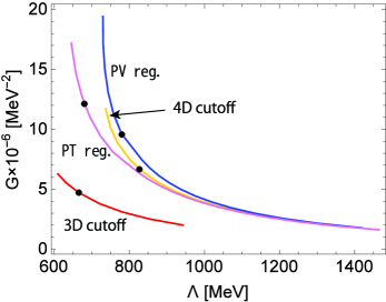
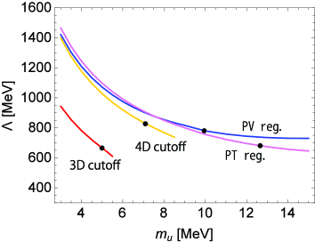
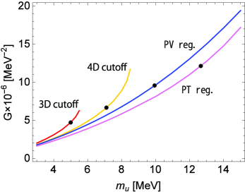
We plot the parameters of each regularization in Fig.1. The black circles denote the value which satisfy MeV for each regularization. The relation between the cutoff scale and for the D cutoff, Pauli-Villars regularization and proper-time regularization resembles each other. The relation between and for these regulatizations also resembles each other. In the case of same value for , the dependence of is large. However, the values of are close, MeV. In the case of same value for , the dependence on is large and the values of are separate in each regularization. The relation between and is different in each regularization.
IV.2 Parameter fitting in the dimensional regularization
For the sake of the parameter fitting in the DR, we present the calculation of the pion to two photon decay rate, , in this subsection. The decay rate can be evaluated through the following one-loop amplitude, ,
| (85) | |||
| (86) |
where is the QED coupling constant and and are the external momentum of emitted photons so the square of the total momentum coincides with that of the original pion, namely, . By using , the decay rate, , is expressed as
| (87) |
The detailed derivation is presented in the paper Krewald:1991tz . After some algebra, one obtains
| (88) |
with , and .
With the observables, , and
| (89) |
we perform the parameter fitting in the DR following Krewald:1991tz . Table. 5 shows the fitted parameters in the DR case.
| (MeV) | (MeV-2) | (MeV) | (MeV) | (MeV) | |
|---|---|---|---|---|---|
| 3.0 | 2.37 | 110 | |||
| 5.0 | 2.56 | 97 | |||
| 8.0 | 2.78 | 80 | |||
| 20.9 | 3.32 | 37 |
We note that both the constituent quark mass and chiral condensate grow up with increasing , which is the characteristic feature in this regularization Inagaki:2010nb .
V Meson properties
We have presented the required equations in the model, then set the parameters for various regularizations. It is now ready for the actual numerical analysis on the model predictions. Here we shall show the thermal meson properties, which are the pion mass, the pion decay constant, and the sigma meson mass.
At finite temperature, there are two ways of the application of each regularization; one is to apply the regularization only for the temperature independent contribution because the temperature dependent contributions are always finite due to the characteristic factor of the Fermi-Dirac distribution, i.e., . The other is to apply the regularization both for the temperature independent and dependent parts, since the regularization essentially relates to the cutoff of the model so the introduction of the same cutoff clearly determines the model scale. On the other hand, the former method retains more symmetry of the model. Then the physical meaning of these prescriptions are that the former one respects the model symmetry, and the latter does the cutoff scale of the model. Since the model is not renormalizable, the predictions depend on the regularization ways and our purpose in this paper is to study the regularization dependence on the model. Therefore we shall study all the cases and compare the results among various regularizations.
V.1 Results with regularizing -independent contribution
In this subsection, we show the results of meson properties based on the procedure of applying the regularization only to the temperature independent part. The required integrals are and , and we evaluate the following combination,
| (90) |
where is for . The lower index indicates each regularization, namely, , , , and . For the temperature dependent part , here we use the form shown in Eq. (24). Similarly for , we use the equivalent expression,
| (91) |
with for each regularization way.
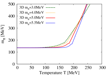
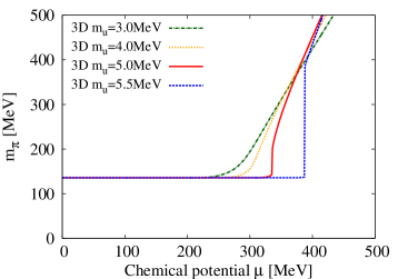
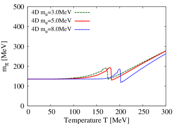
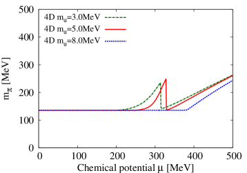
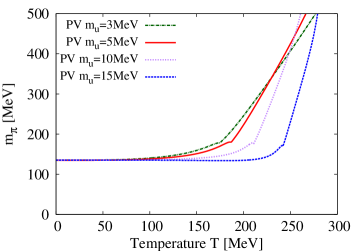
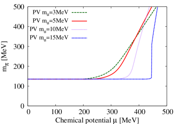
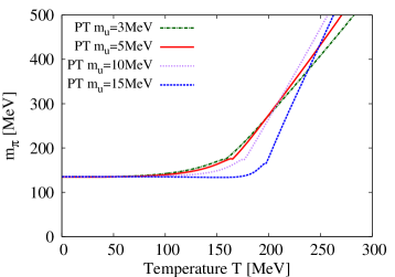
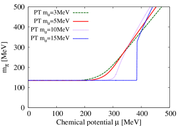
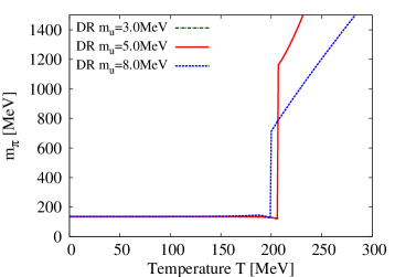
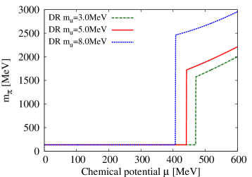
Figure 2 shows how the pion mass changes with respect to and for various parameter sets in the previous section. It should be noted that, for some parameter sets, no real solution exists at high temperature as seen in the case with the DR and MeV Inagaki:2011uj . We observe the similar behavior in each regularization; the pion mass remains almost constant for low and , then raises up for higher and . This comes from the fact that the chiral symmetry is broken at low and and restores at high and . The pion has smaller mass when the symmetry is broken due to the Nambu-Goldstone theorem, while the mass becomes large after symmetry restoration. We see that the mass starts to increase around MeV which is comparable to the critical temperature for the chiral symmetry breaking. We see that the temperature and chemical potential where the pion mass glows up become larger with respect to for the 3D cutoff, 4D cutoff, PV and PT, while they become smaller for the DR. We also see that the discontinuity seen around the transition temperature is considerably larger in the DR case compare to the other regularizations. Then we expect that the tendency of the first order phase transition is strong for the DR comparing the other regularizations. We will discuss it in the next section.
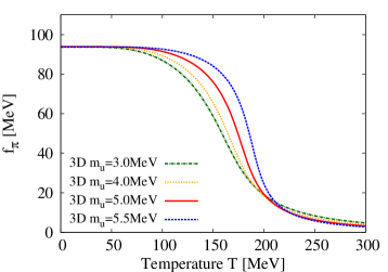
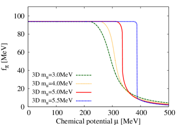
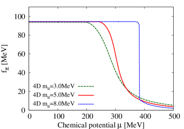
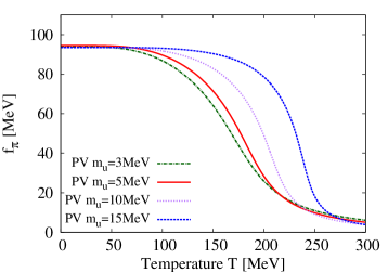
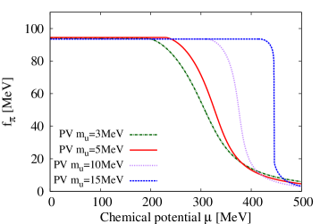
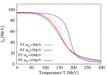
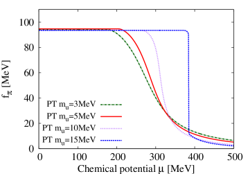
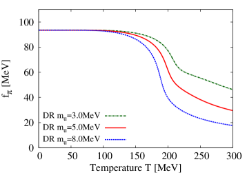
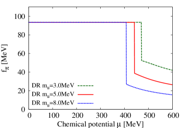
The results of the pion decay are shown in Fig. 3. One sees the similar tendency as well; the decay constant is almost constant for low and , and it decreases when and exceed certain values which are around MeV and MeV. It is interesting to note that the decay constant drops discontinuously at high for some parameter sets in the D, D, PV, PT regularizations, while the discontinuity is always the case in the DR. The existence of the gap is the signal of the first order phase transition, and the tendency becomes stronger with increasing . This is because the coupling strength is larger for higher as seen from the parameter tables, so quarks have stronger correlations when the parameter is larger in the D, D, PV, PT cases.
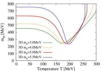
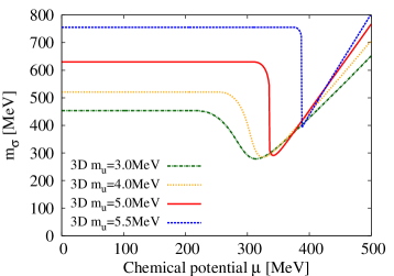
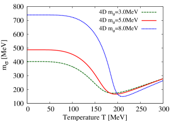
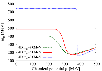
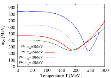
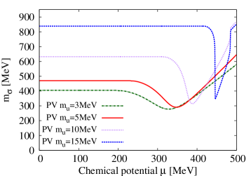
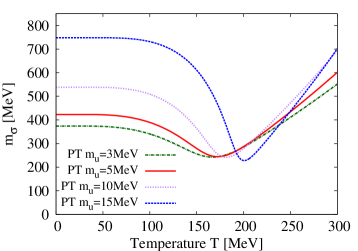
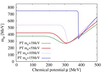
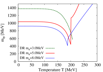
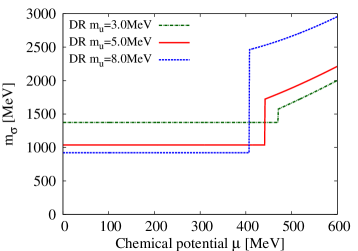
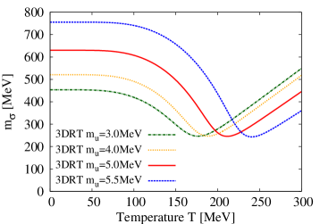
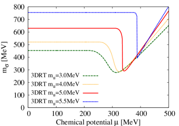
Having fixed the parameters with the pion mass and decay constant. We will calculate the sigma meson mass. It is one of the predictions of the model. Figure 4 shows the numerical results of the sigma mass. At and we find the band around MeV in D, D, PV, PT regularizations, MeV in the DR. Then, in the DR case, the predicted values are larger than the experimental value MeV Agashe:2014kda , in the leading order of the expansion. As is known we can obtain much smaller sigma meson width in this order. We should also check the next to leading order contributions for the sigma meson mass and width. The features of the curves are the similar to that of the pion; the mass decreases with increasing and until some values, then it increases after exceeding the certain values. As seen in the pion mass case, the solution of the sigma mass on the real axis disappears for some parameter set at high temperature.
V.2 Results with regularizing all contribution
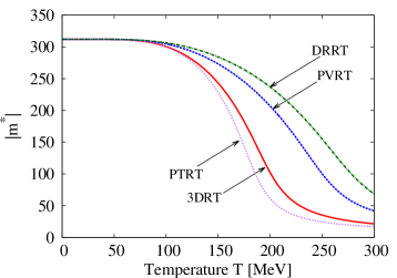
In this subsection, we study the meson properties by applying each regularization procedure to both temperature dependent and independent contributions. It is worth mentioning that the case with D cutoff method does not give credible results because enough number of frequency summations is not taken in this method. The cutoff scale of the D case is around GeV, which means that at MeV only four terms in the Matsubara mode summation, (), are taken into account. It is known that finite temperature field theory does not lead reliable predictions when the number of the frequency summation is small Chen:2010sy . Therefore, we will not show the results in the case of D cutoff scheme here, and consider the other four cases D, PV, PT and DR and call these cases DRT, PVRT, PTRT and DRRT, respectively. It is also worth mentioning that the calculations technically become impossible at in the PTRT case as can be read from Eqs. (67) and (72). Then, we will show the results with as the representative values on dependence at low .
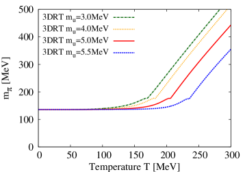

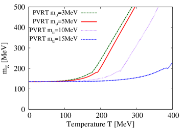
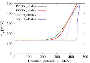
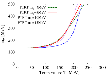
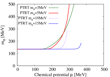
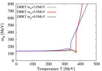
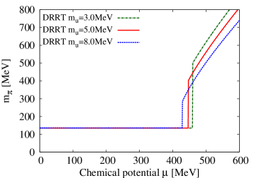
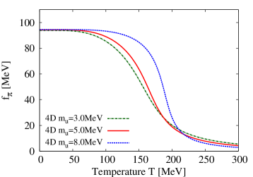
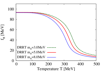
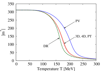
Figure 5 displays the results of the pion mass. One sees that the qualitative feature does not change comparing to the previous case with regularizing only the temperature independent contributions. Quantitatively, we note that the changes become smoother at high and . This can easily be understood because the regularization procedure suppresses the thermal contribution, so the finite temperature term reduces to give smoother curve with respect to and .
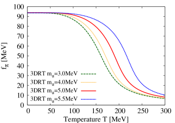
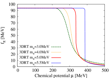
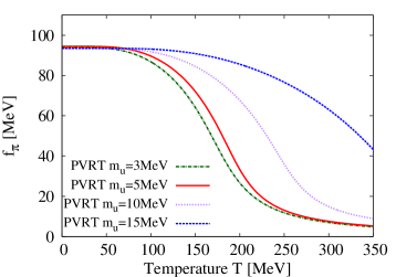
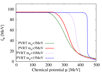
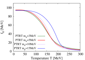
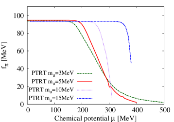
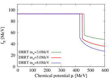
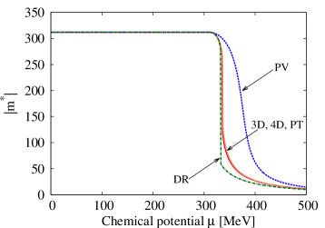
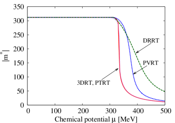
We aligned the results of the pion decay constant in Fig. 6. As seen in the pion mass case, the numerical results do not alter qualitatively, the curves become smooth. Note that, although the dependence becomes considerably smother, the transition chemical potential does not change. This is due to the fact that finite temperature contributions become proportional to the step function for , then the transition chemical potential is not affected by the regularization procedure in this model treatment.
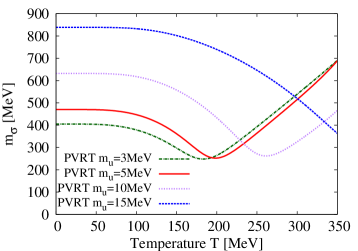
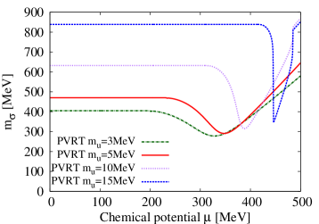
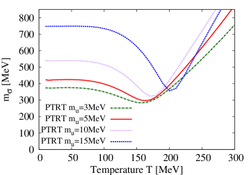
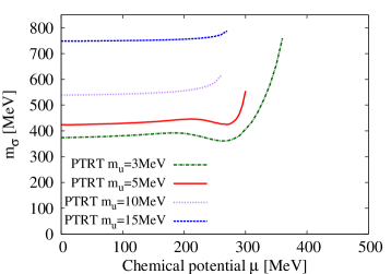
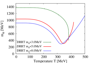
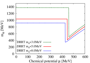
The predictions on the sigma meson mass are shown in Fig. 7. The deviations from the results in the previous subsection in Fig. 4 are more or less similar to the deviations on the pion mass; the curves become flatter with respect to while dependence does not indicate much difference for the D, PV and PT cases. However, there appears substantial difference between the cases of the DR and DRRT where the values of the sigma meson mass at MeV are around MeV for the DR and around MeV for the DRRT case. This comes from the difference of the integral values between these two cases, which we will discuss in more detail in Sec. VIII.
We find that the solution on the real axis always disappears for high and low in the PTRT with , MeV. This is because for high some quantities become pure imaginary number in the calculation due to the complicated counter integral of as seen in Eq. (72). Then one can not find a real solution in that case. This is the numerical reason why the meson properties behave badly for high in PTRT case.
VI Phase diagram
We shall draw the phase diagram in this section. We search the phase transition point by the condition that the maximum change of the chiral condensate with respect to and . In more concrete, we numerically differentiate the condensate with respect to , then the condition can be written
| (92) |
We should be careful on the case with the first order transition, because the condensate has the discontinuous point where we need to find the minimum of the thermodynamic potential then determine the chiral condensate. No matter whether the phase transition is the first order or cross over, we can also use the above criterion since at the first order point, holds, therefore it is consistent in both cases.
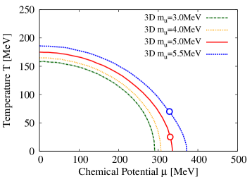
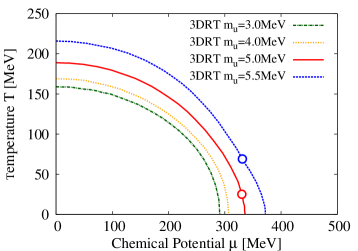
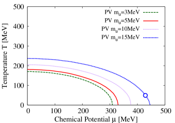
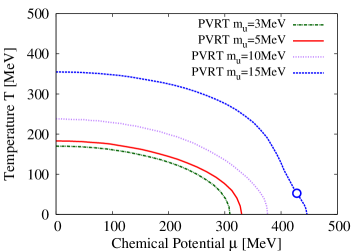
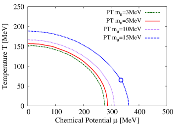
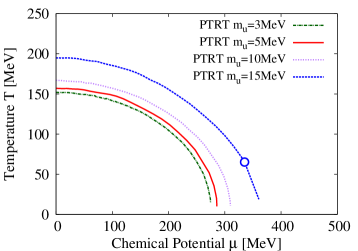
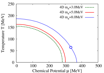
By searching the maximum number of the differentiate of the chiral condensate following the condition Eq. (92), we draw a phase boundary for the chiral symmetry. Figure 8 shows the phase diagrams for the various parameter sets and regularizations. One sees that the critical temperatures, is found between and MeV at if we regularize only the temperature independent parts (left four panels and the bottom panel). On the other hand, a higher critical temperature is observed when the regularization is applied to the temperature dependent and independent parts. The regularizations DRT and PTRT give a critical temperature around MeV at , the PVRT induces a higher critical temperature near MeV with MeV, and the DRRT indicates it around MeV. One also sees that the critical chemical potential, , has no large dependence on the application of the regularization to finite temperature term, because the terms are dominated by the step function as mentioned in the previous section. Consequently, the area of phase boundary enlarges in the direction when we apply the regularization to the temperature dependent term, which is numerically confirmed by the figure.
We think the most interesting comparison from the figure is on the existence of the critical end point where the first order phase transition starts on the phase boundary. For D, D, PV, PT, no critical end point appears for the parameter sets with small . While the critical end point always appears in DR. Then we can numerically conclude that the DR has stronger tendency of the first order phase transition comparing with the other regularizations. The existence of the critical end point in the other four regularizations can be understood by seeing the value of the parameter . Briefly speaking, the critical end point appears when is large. This is physically reasonable because represents the strength of the correlation between quarks, then the larger makes the condensation stronger.
VII Phase diagram with fixing
We have seen the phase diagram and how the location of the critical end point depends on the parameters in the various regularizations. Considering the fact that the transition and is essentially determined by the value of the constituent quark mass since its dependence appears in the thermal distribution, , with , we think it may as well be interesting to compare the phase diagram with the parameter sets which lead the same value of (MeV) at and instead of fixing the current quark mass, .
First, we see the results based on the one with regularizing only the temperature independent parts, 3D, 4D, PV, PT and DR. The behaviors of for each regularization are shown in Fig. 9. All the results have no large difference, because the gap equations of the temperature independent part for each regularization has the similar behavior. The gap equations contain the following form,
| (93) |
in the regularizations, 3D, 4D, PV and PT. While in DR and are replaced by and in some parts (see appendix B). In Fig. 9, we note that the results almost coincide in three regularizations, 3D, 4D and PT. The behavior in PV shows a smaller and DR gives steeper slope than the others.
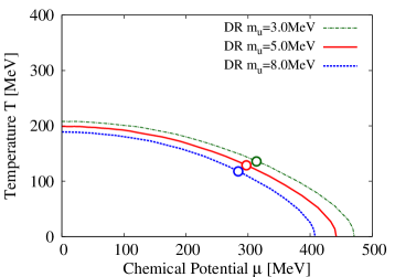
In Fig. 10 the phase diagram is illustrated in each regularization. The phase boundaries of 3D, 4D and PT show almost equivalent behavior. The area of the chiral symmetry broken phase for PV is larger than the others. This tendency comes from the behavior of in Fig. 9. Since the is entered in the form of the dynamical mass, the chiral symmetry breaking contribution is enhanced than the other regularizations. The area for the chiral symmetry broken phase for the DR is smaller than the others. The critical end point for the DR locates higher temperature than the one for 3D, 4D and PT. These tendency also comes from the behavior of in Fig. 9.
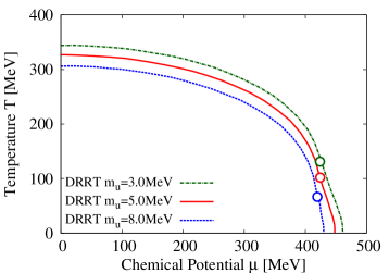
Next, we discuss the results with regularizing both the temperature independent and dependent parts, 3DRT, PVRT, PTRT and DRRT. The behavior of for each regularization is shown in Fig. 11. We find that the finite temperature effect becomes smaller or softer than 3D, PV, PT and DR, respectively. The behavior of in DRRT is the most closest behavior to the case of its regularizing only temperature independent part.
The chemical potential has the similar contribution for 3DRT, PTRT, and PVRT. The behaviors of in DRRT and DR have large difference. This difference is caused by the reduction of the momentum integral dimension, , from to .
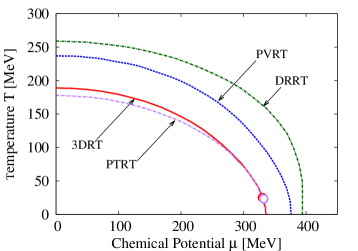
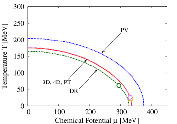
The phase diagram in each regularization is shown in Fig. 12. To compare with Fig. 10, the region of the broken phase enlarges in PTRT, 3DRT and PVRT for a low chemical potential. However, the critical chemical potentials in PTRT, 3DRT and PVRT for a low temperature are almost equivalent to that in PT, 3D and PV, respectively. From the behavior of in Fig. 11, we observe a larger critical temperature and chemical potential for DRRT. We display the location of the critical end points for each regularization in Table.6.
| Regularization | (MeV) | (MeV) |
|---|---|---|
| 3D | 330 | 25.0 |
| 4D | 333 | 46.8 |
| PT | 330 | 26.0 |
| DR | 289 | 74.7 |
| 3DRT | 330 | 25.0 |
| PTRT | 332 | 23.2 |
VIII Discussions
We have introduced the regularization methods then studied the meson properties and phase diagram in previous sections. In this section, we are going to present more detailed discussions on the obtained results.
In comparing the left panels v.s. right panels in Fig. 8, one can observe the contribution to apply the regularization procedure to the thermal correction. The phase diagram does not show considerable difference for D and PT cases, while in PV the area of the phase boundary becomes larger in the right panel when is large, and the areas in DRRT case is larger than DR case for all the parameter sets. These difference can be understood through the following discussion.
The loop integral, , essentially has the following subtracted forms for DRT, PVRT, and PTRT,
| (94) | |||
| (95) | |||
| (96) |
Where the typical form of is given by with some constant value, . Thus the subtracted terms basically relate to the suppression on the high energy contributions which are expected to be small. We numerically confirmed that the subtracted parts are small for almost all the cases, then the phase diagrams does not change drastically. However, in the PV case with large , the difference between and is small since the constituent quark mass becomes comparable to the cutoff scale, e.g., MeV and MeV for MeV in PV. Consequently, the thermal contribution strongly suppressed in the PV case with large .
We saw that the area of the phase boundary does not alter so much in D, PV and PT regularizations. The essential reason is that the infinities appearing from loop integrals are subtracted at high energy. However in DR, the situation is different since the integral is replaced as
| (97) |
so this modifies the integral kernel rather than the subtraction of high energy modes. This is the reason why DR shows considerable difference, if we apply the regularization to both temperature independent and dependent contributions.
We also saw the location (or existence) of the critical end point is non-trivial. In Fig. 10, the diagram has the critical end point for D, D, PT and DR. No critical end point appears in the PV. Thus we find that the PV has weaker tendency of the first order phase transition than that of the other regularization methods. Particularly, the temperature of the critical end point in the DR case is higher then others, which may enable us to conclude that the DR has the stronger tendency of the first order phase transition.
IX Concluding remarks
We have studied the regularization dependence on the phase diagram of quark matter on plane by using the NJL model. We have first presented the regularization procedure at finite temperature and chemical potential, then fitted parameters within various regularization methods. Thereafter, we have studied the meson properties and the phase structure.
We find that the model produces the reliable predictions on the meson properties whose behavior for finite temperature and chemical potential does not alter drastically, which indicates that all the regularizations employed in this paper nicely capture physics on the meson properties. We can conclude that the regularizations are safely adopted. In this context the regularization parameter independent approach is also interesting inagaki:2013 ; inagaki:2014 .
It is expected that observation of the critical end point can distinguish a suitable regularization for an effective model of QCD by comparing with the resulting phase diagrams. The important difference is the existence of the critical end point. The model predicts that the critical end point appears at intermediate chemical potential around MeV. This density coincides the one in which different quark state such as color superconductivity may occur, there the order of the phase transition might affect crucially on such the dense states. Moreover the color superconductivity may be realized in the dense stellar objects, like quark stars and neutron stars fujihara:2009 . Therefore the study of the order of the phase transition has important meaning as well in cosmological observations. So we believe that the further and more extensive investigations are necessary on this subject.
Acknowledgements.
TI is supported by JSPS KAKENHI Grant Number 26400250. HK is supported by MOST 103-2811-M-002-087.Appendix A Analytic expressions for
Since the integral can be evaluated analytically, we will present the explicit expression for various regularizations.
One needs special care in performing integral since it contains divergent contribution as seen in the 3D cutoff scheme. becomes for ,
| (98) |
and for ,
| (99) |
where
| (100) |
Concerning on , it is convenient that we divide the integral as
| (101) |
where is subtracted part in the original integral and it becomes
| (102) |
with
| (103) |
As seen above, we need to separately evaluate the integral depending on the values of and . It becomes for ,
| (104) |
and for ,
| (105) |
where
| (106) |
Appendix B and for
We arrange the concrete expressions for and .
For we have
| (107) | |||||
| (108) |
For we have
| (109) | |||||
| (110) |
For we have
| (111) | |||||
| (112) |
References
- (1) M. A. Stephanov, Prog. Theor. Phys. Suppl. 153, 139 (2004), Int. J. Mod. Phys. A 20, 4387 (2005), PoS LAT 2006, 024 (2006), O. Philipsen, Prog. Theor. Phys. Suppl. 174, 206 (2008), arXiv:1111.5370 [hep-ph], W. Weise, Prog. Theor. Phys. Suppl. 186, 390 (2010), arXiv:1201.0950 [nucl-th], K. Fukushima and T. Hatsuda, Rept. Prog. Phys. 74, 014001 (2011), G. Endrodi, Z. Fodor, S. D. Katz and K. K. Szabo, JHEP 1104, 001 (2011).
- (2) D. Gross and F.Wilczek, Phys. Rev. Lett. 30, 1343 (1973).
- (3) K. G. Wilson, Phys. Rev. D 10, 2445 (1974).
- (4) Y. Nambu and G. Jona-Lasinio, Phys. Rev. 122, 345 (1961); 124, 246 (1961).
- (5) U. Vogl and W. Weise, Prog. Part. Nucl. Phys. 27, 195 (1991).
- (6) S. P. Klevansky, Rev. Mod. Phys. 64, 649 (1992).
- (7) T. Hatsuda and T. Kunihiro, Phys. Rept. 247, 221 (1994).
- (8) M. Buballa, Phys. Rept. 407, 205 (2005).
- (9) M. Huang, Int. J. Mod. Phys. E 14, 675 (2005).
- (10) W. Pauli and F. Villars, Rev. Mod. Phys. 21 434 (1949).
- (11) C. Itzykson and J. B. Zuber, Quantum Field Theory (McGrow-Hill Inc. Press, 1980).
- (12) T. P. Cheng and L. F. Li, Gauge Theory of Elementary Particle Physics (Oxford University Press, 1984).
- (13) J. S. Schwinger, Phys. Rev. 82 664 (1951).
- (14) G. ’t Hooft and M. J. G. Veltman, Nucl. Phys. B 44 189 (1972).
- (15) D. Kahana and M. Lavelle, Phys. Lett. B 298 397 (1993).
- (16) A. A. Osipov, H. Hansen and B. Hiller, Nucl. Phys. A 745 81 (2004).
- (17) J. Moreira, B. Hiller, A. A. Osipov and A. H. Blin, Int. J. Mod. Phys. A 27 1250060 (2012).
- (18) H. Suganuma and T. Tatsumi, Annals Phys. 208 470 (1991).
- (19) K. G. Klimenko, Theor. Math. Phys. 89 1161 (1992) [Teor. Mat. Fiz. 89 211 (1991)].
- (20) K. G. Klimenko, Z. Phys. C 54 323 (1992).
- (21) V. P. Gusynin, V. A. Miransky and I. A. Shovkovy, Phys. Rev. Lett. 73 3499 (1994) [Erratum-ibid. 76 1005 (1996)].
- (22) T. Inagaki, S. D. Odintsov and Y. I. Shil’nov, Int. J. Mod. Phys. A 14 481 (1999).
- (23) T. Inagaki, D. Kimura and T. Murata, Prog. Theor. Phys. Suppl. 153 321 (2004).
- (24) T. Inagaki, D. Kimura and T. Murata, Prog. Theor. Phys. 111 371 (2004).
- (25) T. Inagaki, D. Kimura and T. Murata, Int. J. Mod. Phys. A 20 4995 (2005).
- (26) Z. F. Cui, Y. L. Du and H. S. Zong, Int. J. Mod. Phys. Conf. Ser. 29 1460232 (2014).
- (27) S. Krewald and K. Nakayama, Annals Phys. 216, 201 (1992).
- (28) R. G. Jafarov and V. E. Rochev, Central Eur. J. Phys. 2, 367 (2004).
- (29) R. G. Jafarov, and V. E. Rochev, Russ. Phys. J. 49, 364 (2006), Izv. Vuz. Fiz. 49, 20 (2006).
- (30) T. Inagaki, D. Kimura and A. Kvinikhidze, Phys. Rev. D 77, 116004 (2008).
- (31) T. Inagaki, D. Kimura, H. Kohyama and A. Kvinikhidze, Phys. Rev. D 85, 076002 (2012).
- (32) T. Inagaki, D. Kimura, H. Kohyama and A. Kvinikhidze, Phys. Rev. D 86, 116013 (2012).
- (33) T. Fujihara, D. Kimura, T. Inagaki and A. Kvinikhidze, Phys. Rev. D 79, 096008 (2009).
- (34) M. Asakawa and K. Yazaki, Nucl. Phys. A 504, 668 (1989).
- (35) T. Inagaki, T. Kouno and T. Muta, Int. J. Mod. Phys. A10, 2241 (1995).
- (36) T. Inagaki, D. Kimura, H. Kohyama and A. Kvinikhidze, Phys. Rev. D 83, 034005 (2011).
- (37) K. A. Olive et al. [Particle Data Group Collaboration], Chin. Phys. C 38, 090001 (2014).
- (38) J. W. Chen, H. Kohyama and U. Raha, Phys. Rev. D 83, 094014 (2011) [arXiv:1009.4456 [hep-ph]].
- (39) T. Inagaki, D. Kimura, H. Kohyama and A. Kvinikhidze, Int. J. Mod. Phys. A28, 1350164 (2013).
- (40) T. Inagaki, D. Kimura and H. Kohyama, Int. J. Mod. Phys. A29, 1450048 (2014).