The Imaginary Potential and Thermal Width of Moving Quarkonium from Holography
Kazem Bitaghsir Fadafan, Seyed Kamal Tabatabaei

Physics Department, Shahrood University, Shahrood, Iran

We study the effect of finite ’t Hooft coupling corrections on the imaginary potential and the thermal width of a moving heavy quarkonium from the AdS/CFT correspondence. To study these corrections, we consider $\mathcal{R}^{4}$ terms and Gauss$-$Bonnet gravity. We conclude that the imaginary potential of a moving or static heavy quarkonium starts to be generated for smaller distances of quark and antiquark. Similar to the case of static heavy quarkonium, it is shown that by considering the corrections the thermal width becomes effectively smaller. The results are compared with analogous calculations in a weakly coupled plasma.

1 Introduction

In heavy ion collisions at the LHC and RHIC, heavy quark related observables are becoming increasingly important [1]. In these collisions, one of the main experimental signatures of the formation of a strongly coupled quark$-$gluon plasma (QGP) is melting of quarkonium systems, like $J/\psi$ and excited states, in the medium. In this case, the main mechanism responsible for this suppression is color screening [2]. Recent studies suggest a more important reason than screening, which is the existence of an imaginary part of the potential [3, 4]. Then the thermal width of these systems is an important subject in QGP. In the effective field theory framework, thermal decay widths have been studied in [5, 6]. It was shown that at leading order, two different mechanisms contribute to the decay width, namely Landau damping and singlet-to-octet thermal breakup [7]. The analytic estimate of the imaginary part of the binding energy and the resultant decay width were studied in [8]. The peak position and its width in the spectral function of heavy quarkonium can be translated into the real and imaginary part of the potential [9]. The effect of the imaginary part of the potential on the thermal widths of the states in both isotropic and anisotropic plasmas has been studied in [10].

In heavy ion collisions, most of quarkonium observed experimentally are moving through the medium with relativistic velocities. They have finite probability to survive, even at infinitely high temperature. Two mechanisms of charmonium attenuation by considering final state interactions have been studied in [11]. The bottomium suppression in PbPb collisions at LHC energies is studied in [12]. Study of heavy quarkonium moving in a quark-gluon plasma from effective field theory techniques has been done in [14, 13]. It is shown that in the regime relevant for dissociation and for very large velocities the thermal width decreases with increasing velocity of quarkonium [14].

A new method for studying different aspects of QGP is the AdS/CFT correspondence [15]. This method has yielded many important insights into the dynamics of strongly coupled gauge theories. It has been used to study hydrodynamical transport quantities at equilibrium and real$-$time processes in non-equilibrium [16]. Methods based on AdS/CFT relate gravity in $AdS_{5}$ space to the conformal field theory on the four-dimensional boundary [17]. It was shown that an $AdS$ space with a black brane is dual to a conformal field theory at finite temperature [18].

We have studied the imaginary potential and the thermal width of static quarkonium from the AdS/CFT correspondence in [19]. These quantities initially studied in [20]. In this approach, the thermal width of heavy quarkonium states originates from the effect of thermal fluctuations due to the interactions between the heavy quarks and the strongly coupled medium. This method was revisited in [21] and general conditions for the existence of an imaginary part for the heavy quark potential were obtained. In the context of AdS/CFT, there are other approaches which can lead to a complex static potential [22, 23]. The case of anisotropic plasma has been studied in [24, 25] and imaginary potential formula in a general curved background was obtained. It was also shown that the thermal width is decreased in presence of anisotropy and bigger decrease happens along the transverse plane. With using a probe D7-brane in the dual gravity theory, thermal width is investigated in [26]. The effects of deformation parameter on thermal width of moving quarkonium has been studied in [27].

The imaginary potential and the thermal width of a moving heavy quark$-$antiquark pair in an isotropic plasma, depend on the angle $\theta$ between the direction of the pair and the velocity of the wind $v$ . Then it would be possible to consider different alignments for quark$-$antiquark pair with respect to the plasma wind. They are parallel ($\theta=0$), transverse ($\theta=\pi/2$) or arbitrary direction to the wind ($\theta$). By increasing the angle from zero to $\pi/2$ the imaginary potential and the thermal width for a fixed velocity is changing. We will examine this idea in the presence of higher derivative corrections. Including the higher derivative corrections would be important from a phenomenology point of view. Two extreme cases, transverse and parallel to the wind have been studied in [28]. The case where the axis of the moving pair has an arbitrary orientation with respect to the wind has been done in [29]. It should be noticed that the extreme cases are much simpler than arbitrary case to study. In this article, we have studied all cases.

Using the AdS/CFT correspondence, we have studied melting of a heavy meson like $J/\psi$ and excited states like $\chi_{c}$ and $\psi^{\prime}$ in the quark medium in [30]. It was shown that the excited states melt at higher temperatures. Also heavy quarks in the presence of higher derivative corrections have been studied in [31, 32]. In this paper, we continue our study in [19] to a moving quarkonium. Finite ’t Hooft coupling corrections have been considered. These corrections correspond to $\mathcal{R}^{4}$ corrections and Gauss$-$Bonnet terms, respectively. An understanding of how the imaginary part of the potential and the thermal width of heavy quarkonium are affected by these corrections may be essential for theoretical predictions. Actually, to study more realistic models we added higher derivative Gauss$-$Bonnet corrections. They are the leading $1/N_{c}$ corrections in the presence of a D7-brane. It has been shown that these type of corrections can increase the nuclear modification factor $R_{AA}$ [33, 34].

We compare our results with static case and conclude that the imaginary potential of a moving or static heavy quarkonium starts to be generated for smaller distances of quark and antiquark. Also similar to the case of static heavy quarkonium, it is shown that by considering these corrections the thermal width becomes effectively smaller. The same results also can be found in calculations in a weakly coupled plasma [14].

This paper is organized as follows. In the next section, we will present the finite coupling corrections. We give the general expressions to study the imaginary potential and the thermal width for ($\theta=\pi/2$) in Sect. 3. For ($\theta=0$) and arbitrary angle ($\theta$), we address the relevant papers and concern mainly on the results. Also in this section, we show the effect of the corrections in the different plots. The thermal width behavior has been explored in Sect. 4. We discuss the limitations of the method, too. In the last section we summarize our results.

2 On finite coupling corrections

One may consider the general gravity as follows:

$$ds^{2}=G_{tt}dt^{2}+G_{xx}dx_{i}^{2}+G_{uu}du^{2},$$ (2.1)

here the metric elements are functions of the radial distance $u$ and $x_{i}=x,y,z$ are the boundary coordinates. In these coordinates, the boundary is located at infinity.

From the AdS/CFT, the coupling which is denoted as ’t Hooft coupling $\lambda$ is related to the curvature radius of the $AdS_{5}$ and $S_{5}$ $(R)$, and the string tension $(\frac{1}{2\pi\alpha^{\prime}})$ by $\sqrt{\lambda}=\frac{R^{2}}{\alpha^{\prime}}$. A general result of the AdS/CFT correspondence states that the effects of finite but large $\lambda$ coupling in the boundary field theory are captured by adding higher derivative interactions in the corresponding gravitational action. In our study, the corrections to the AdS-Schwarzschild black brane are $\mathcal{R}^{4}$ and $\mathcal{R}^{2}$ corrections.

• $\mathcal{R}^{4}$ corrections:

Since the $AdS/CFT$ correspondence refers to complete string theory, one should consider the string corrections to the 10D supergravity action. The first correction occurs at order $(\alpha^{\prime})^{3}$ [35]. In the extremal $AdS_{5}\times S^{5}$ it is clear that the metric does not change [36]; conversely this is no longer true in the non-extremal case. Corrections in inverse ’t Hooft coupling $1/\lambda$, which correspond to $\alpha^{\prime}$ corrections on the string theory side, were found in [35]. The functions of the $\alpha^{\prime}$-corrected metric are given by [37]

$$G_{tt} = -u^{2}(1-w^{-4})T(w),$$

$$G_{xx} = u^{2}X(w),$$

$$G_{uu} = u^{-2}(1-w^{-4})^{-1}U(w),$$ (2.2)

where

$$T(w) = 1-k\bigg{(}75w^{-4}+\frac{1225}{16}w^{-8}-\frac{695}{16}w^{-12}\bigg{)}+\dots,$$

$$X(w) = 1-\frac{25k}{16}w^{-8}(1+w^{-4})+\dots,$$

$$U(w) = 1+k\bigg{(}75w^{-4}+\frac{1175}{16}w^{-8}-\frac{4585}{16}w^{-12}\bigg{)}+\dots,\$$ (2.3)

and $w=\frac{u}{u_{h}}$. There is an event horizon at $u=u_{h}$ and the geometry is asymptotically $AdS$ at large $u$ with a radius of curvature $R=1$. The expansion parameter $k$ can be expressed in terms of the inverse ’t Hooft coupling as

$$k=\frac{\zeta(3)}{8}\lambda^{-3/2}\sim 0.15\lambda^{-3/2}.$$ (2.4)

The temperature is given by

$$T=\frac{u_{h}}{\pi R^{2}(1-k)}.$$ (2.5)

• $\mathcal{R}^{2}$ corrections:

In five dimensions, we consider the theory of gravity with quadratic powers of curvature as Gauss$-$Bonnet (GB) theory. The exact solutions and thermodynamic properties of the black brane in GB gravity are discussed in [38, 39, 40]. The metric functions are given by

$$G_{tt}=-N\,u^{2}\,h(u),\,\,\,\,\,\,G_{uu}=\frac{1}{u^{2}h(u)},\,\,\,\,\,G_{xx}=G_{yy}=G_{zz}=u^{2},$$ (2.6)

where

$$h(u)=\frac{1}{2\lambda_{GB}}\left[1-\sqrt{1-4\lambda_{GB}\left(1-\frac{u_{h}^{4}}{u^{4}}\right)}\right].$$ (2.7)

In (2.6), $N=\frac{1}{2}\left(1+\sqrt{1-4\lambda_{GB}}\right)$ which is an arbitrary constant that specifies the speed of light of the boundary gauge theory and we choose it to be unity. Beyond $\lambda_{GB}<1/4$ there is no vacuum AdS solution and one cannot have a conformal field theory at the boundary. Causality leads to new bounds for the value of the Gauss$-$Bonnet coupling constant as $-7/36<\lambda_{GB}<9/100$ [41]. In our method for computing the thermal width, we find that only positive values of $\lambda_{GB}$ is valid. The temperature also is given by

$$T=\sqrt{N}\,\frac{u_{h}}{\pi R^{2}}.$$ (2.8)

Also the ’t Hooft coupling of the dual strongly coupled CFT is $\lambda=\frac{N^{2}R^{4}}{\alpha^{\prime 2}}$ .

3 Finding the imaginary potential

In our study, we assume that the quark$-$antiquark pair is moving with rapidity $\eta$. One should notice that in our reference frame the plasma is at rest. Then we boost the frame in the $x_{3}$ direction with rapidity $\eta$ so that $dt^{\prime}=dt^{\prime}\cosh\eta-dx^{\prime}_{3}\sinh\eta$ and $dx_{3}=-dt^{\prime}\sinh\eta+dx^{\prime}_{3}\cosh\eta.$ After dropping the primes, the metric becomes

$$ds^{2}= -\left(|G_{tt}|\cosh^{2}\eta-G_{xx}\sinh^{2}\eta\right)dt^{2}+\left(G_{xx}\cosh^{2}\eta-|G_{tt}|\sinh^{2}\eta\right)dx_{3}^{2}$$

$$-2\,\sinh\eta\,\cosh\eta\left(G_{xx}-|G_{tt}|\right)\,dt\,dx_{3}+G_{xx}(dx_{1}^{2}+dx_{2}^{2})+G_{uu}du^{2},$$ (3.1)

We define new metric functions as follows:

$$\tilde{W}(u)\equiv W(u)\cosh^{2}\eta-N(u)\sinh^{2}\eta$$ (3.2a)

$$\tilde{V}(u)\equiv V(u)\cosh^{2}\eta-P(u)\sinh^{2}\eta$$ (3.2b)

where $V(u)\equiv-|G_{tt}|G_{xx},\,\,\,W(u)\equiv-|G_{tt}|G_{uu},\,\,P(u)=G_{xx}^{2}$ and $N(u)=G_{xx}G_{uu}.$

Now one should use the usual orthogonal Wilson loop, which corresponds to the heavy QQ̄ pair.

3.1 Transverse to the wind ($\theta=\pi/2$)

Assuming the system to be aligned perpendicularly to the wind, in the $x_{1}$ direction

$$t=\tau,\quad x_{1}=\sigma,\quad u=u(\sigma)~{},$$ (3.3)

The distance between $Q\bar{Q}$ pair depends on the velocity and angle, $L(\pi/2,\eta)$, we call it $L$. The quarks are located at $x_{1}=-\frac{L}{2}$ and $x_{1}=+\frac{L}{2}$. One finds the following generic formulas for the heavy meson. In these formulas $u_{*}\equiv u(x=0)$ is the deepest point of the U-shaped string.

• The distance between quark and antiquark, $L$, is given by

  $$L(\pi/2,\eta)=2\,\int_{u_{*}}^{\infty}du~{}\left[\frac{\tilde{V}(u)}{\tilde{W}(u)}\left(\frac{\tilde{V}(u)}{\tilde{V}(u_{*})}-1\right)\right]^{-\frac{1}{2}}.$$ (3.4)

• The real part of heavy quark potential, $ReV_{Q\bar{Q}}(\pi/2,\eta)$ is as follows:

  $$ReV_{Q\bar{Q}}=\frac{1}{\pi\alpha^{\prime}}\left[\int_{u_{*}}^{\infty}du~{}\left(\left(\frac{1}{\tilde{W}(u)}-\frac{\tilde{V}(u_{*})}{\tilde{V}(u)\tilde{W}(u)}\right)^{-1/2}-\sqrt{\tilde{W}_{0}(u)}\right)-\int_{u_{h}}^{u_{*}}du~{}\sqrt{\tilde{W}_{0}(u)}\right],$$

  (3.5)

  here $\tilde{W}_{0}(u)=\tilde{W}(u\rightarrow\infty)$.

• The imaginary part of the potential is negative and it is given by

  $$\text{Im}V_{Q\bar{Q}}(\pi/2,\eta)=-\frac{1}{2\sqrt{2}\alpha^{\prime}}\left[\frac{\tilde{V}^{\prime}(u_{*})}{2\tilde{V}^{\prime\prime}(u_{*})}-\frac{\tilde{V}(u_{*})}{\tilde{V}^{\prime}(u_{*})}\right]~{}\sqrt{\tilde{W}(u_{*})}~{}.$$ (3.6)

  The derivatives are with respect to $u$. For the static quarkonium and special case of $W(u)=1$, this formula reduces to the case of an isotropic plasma [20], while $W(u)\neq 1$ corresponds to the anisotropic plasma [24, 25] .

These generic formulas give the related information of the moving heavy quarkonium in terms of the metric elements of a background (2.1).

To find $\text{Im}V$, one should express it in terms of the length $L$ of the Wilson loop instead of $u_{*}$ using the equation (3.4). There is an important point for long U-shaped strings, because it would be possible to add new configurations [42]. Here we are interested mostly in distances $LT<1$ and do not consider such configurations.

To begin with, we calculate the imaginary potential in the $N=4$ SYM. The metric functions are

$$V(u)=\frac{u^{4}-u_{h}^{4}}{R^{4}},\,\,\,\,\,W(u)=1,\,\,\,P(u)=\frac{u^{4}}{R^{4}},\,\,\,N(u)=\left(1-\frac{u_{h}^{4}}{u^{4}}\right)^{-1}.$$ (3.7)

where the horizon is located at $u_{h}$ and the temperature of the hot plasma is given by $u_{h}=\pi R^{2}T$. In this case we do not consider any correction and find the imaginary potential from (3.6) to be

$$\text{ImV}_{Q\bar{Q}}(\pi/2,\eta)=-\frac{\pi\sqrt{\lambda}\,T}{24\sqrt{2}\xi}\,\sqrt{\frac{1-\xi^{4}cosh^{2}\eta}{1-\xi^{4}}}\left(3\xi^{4}cosh^{2}\eta-1\right),\,\,\,\,\,\,\,\xi=\frac{u_{h}}{u_{*}}.$$ (3.8)

The imaginary potential is negative; it implies that there is a lower bound for the deepest point of the U-shaped string, i.e. $\xi_{min}^{2}=\frac{1}{\sqrt{3}cosh^{2}\eta}$. This minimum value is found by solving $\text{ImV}_{Q\bar{Q}}=0$. The maximum value $\xi_{max}$ occurs when the distance $L$ approaches the maximum value.

  

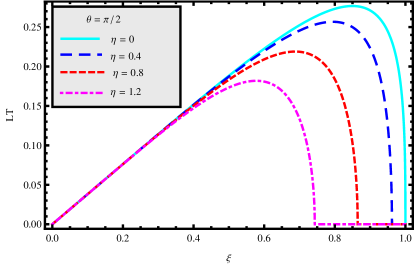
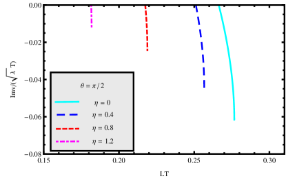
Figure 1: Left: The distance between quark and antiquark versus the $\xi$ when the quarkonium is moving transverse to the wind. Right: The imaginary potential for the valid values of $\xi$ or $L$.

The imaginary potential for accepted values of $\xi$ is shown in the right plot of Fig. 1. It is clearly seen that the imaginary potential starts to be generated at $L_{min}$ or $\xi_{min}$ and increases in absolute value with $L$ until a value $L_{max}$ or $\xi_{max}$. It should be noticed that for $\xi$ very close to the horizon one should consider higher order corrections [42].

3.2 Parallel to the wind $(\theta=0)$

Assuming the system to be aligned parallel to the wind, in the $x_{3}$ direction

$$t=\tau,\quad x_{3}=\sigma,\quad u=u(\sigma)~{},$$ (3.9)

The distance between $Q\bar{Q}$ pair is called again $L$ and quarks are located at $x_{3}=-\frac{L}{2}$ and $x_{3}=+\frac{L}{2}$. One finds the generic formulas for finding $L$ and imaginary potential in [28]. Here, we focus on the resultant plots.

In the left plot of Fig. 2, the distance between quark and antiquark versus the $\xi$ has been shown. The imaginary potential also is given in the right plot of this figure. Comparing the absolute value of imaginary potential in two extreme cases has been done in [28, 29]. It is found that stronger modification occurs when quarkonium is moving orthogonal to the wind. This is similar to the screening length where decreases as the quarkonium is moving transverse with respect to the wind [43]. One finds that by increasing rapidity the imaginary potential happens for smaller LT. Thus, the magnitude of the imaginary potential vanishes for ultra-relativistic moving quarkonium. One important reason for this observation is coming from the saddle point approximation. It was argued that this approximation correspond to large velocity of moving quarkonium [29]. Then one may discuss only the case of slowly moving quarkonium.

  

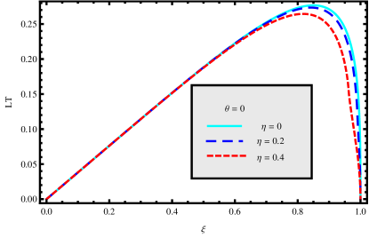
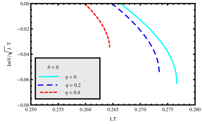
Figure 2: Left: The distance between quark and antiquark versus the $\xi$ when the quarkonium is moving parallel to the wind. Right: The imaginary potential for the accepted values of $\xi$ or $L$.

3.3 Arbitrary angle to the wind ($\theta$)

Assuming the wind in the $x_{3}$ direction, we consider the quarkonium to be aligned arbitrary to the wind as $\theta$ angle. Then the parametrization changes

$$t=\tau,\quad x_{1}=\sigma,\quad x_{3}=x_{3}(\sigma),\quad u=u(\sigma)~{},$$ (3.10)

The distance between $Q\bar{Q}$ pair is called again $L$ and the projections of the system of quarks on the $x_{1}$ and $x_{3}$ direction are of length $L\sin\theta$ and $L\cos\theta$, respectively. In this case, the shape of the string is found by $x_{3}(\sigma)$ and $u(\sigma)$. Especially, the $u(\sigma)$ is not a straight line. More details about the shape of string and solutions are given in [43]. The velocity dependence of the potential also has been discussed. One finds the generic formulas for finding the imaginary potential in [29]. We have done the same calculations as before. We found the distance between quark$-$antiquark ($Q\bar{Q}$) versus the $\xi$ for different angles. Also the imaginary potential for different angles has been studied. For example in the left plots of Fig. 3 and Fig. 4, the $\theta=\pi/3$ has been considered.

One finally concludes the main results about the imaginary potential as follows:

• The imaginary potential strongly depends on the velocity of the moving quarkonium and the angle $\theta$.

• At fixed angle, by increasing the velocity the absolute value of the imaginary potential decreases.

• At fixed velocity, by increasing the $\theta$ the absolute value of the imaginary potential increases.

• The velocity of moving quarkonium has important effect when it is moving transverse to the wind comparing with the parallel motion.

3.4 Finite coupling corrections

• $\mathcal{R}^{4}$ corrections

The distance between the quark and antiquark versus the $\xi$ for different values of the coupling $\lambda$ has been studied. We find that decreasing $\lambda$ leads to decreasing of the maximum value of the quark$-$antiquark distance. This behavior is the same as the static case in Fig. 2 of [19]. The imaginary potential at $(\theta=\pi/3,\eta=.5)$ and $(\theta=0,\eta=.3)$ have been shown in the left and right plot of Fig. 3, respectively. In each plot, we assume $\lambda=8,12,20$. As it was pointed out in the section 2, such corrections decrease the ’t Hooft coupling from infinity to finite number. Thus, turning on $\mathcal{R}^{4}$ corrections leads to generating the imaginary potential for smaller quark$-$antiquark distances. This behavior is the same as the static quarkonium [19].

• Gauss$-$Bonnet corrections

We find that only positive values of $\lambda_{GB}$ are valid in our approach to produce the imaginary potential. The study of the behavior of $L$ in terms of $\xi$ for different values of $\lambda_{GB}$ shows that by increasing the coupling constant the maximum value of $L$ decreases. As in the static case, this behavior is not the same as the $\mathcal{R}^{4}$ corrections [19]. The imaginary potential at $(\theta=\pi/3,\eta=.5)$ and $(\theta=0,\eta=.3)$ have been shown in the left and right plot of Fig. 4, respectively. In each plot, we assume $\lambda_{GB}$=0.04, 0.065, 0.08. The imaginary potential in the Gauss$-$Bonnet gravity starts to be generated for smaller distances. It means that by turning on the Gauss$-$Bonnet coupling, the imaginary potential starts to be generated for smaller distances of quark$-$antiquark. Also the absolute value of the imaginary potential becomes smaller. The effect of higher derivative corrections on the imaginary potential of a static quarkonium has the same behavior [19]. This would be a general feature of higher derivative corrections:

• The imaginary part of the potential of a moving or static heavy quarkonium starts to be generated for smaller distances of quark$-$antiquark.

• The absolute value of the imaginary part of the potential of a moving or static heavy quarkonium becomes smaller.

We call the maximum distance of quark$-$antiquark where the imaginary part of the potential starts as $LT_{max}$. To more clarify the above general results, we plot $LT_{max}$ versus the rapidity $\eta$ in Fig. 5. We see that $LT_{max}$ decreases monotonically with $\eta$. Such a behavior is the same as the $LT_{min}$ for the onset of the imaginary part of the potential, as shown in [29]. It is clearly seen that higher derivative corrections decreases this quantity.

 

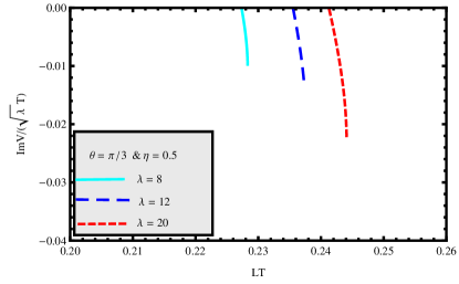
Figure 3: The imaginary potential versus $LT$ in the presence of $\mathcal{R}^{4}$ corrections. Left: $(\theta=\pi/3,\eta=.5)$. Right: $(\theta=0,\eta=.3)$. In each plot we assume $\lambda$= 20, 12, 8.

  

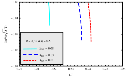
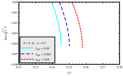
Figure 4: The imaginary potential versus $LT$ in the presence of Gauss$-$Bonnet corrections. Left: From left to right $\lambda_{GB}$=0.08, 0.03, 0.01 and $(\theta=\pi/3,\eta=.5)$. Right: From left to right $\lambda_{GB}$=0.08, 0.065, 0.04 and $(\theta=0,\eta=.3)$.

  

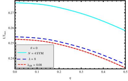
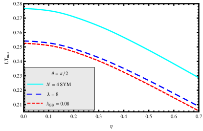
Figure 5: $LT_{max}$ versus the rapidity for different corrections. Left: Parallel to the wind $(\theta=0)$. Right: transverse to the wind $(\theta=\pi/2)$.

4 Thermal width from holography

In this section, we consider the moving quarkonium and compute the corrections on the thermal width from holography. The static case has been studied in [25], it was also pointed out that the imaginary potential for confining geometry is zero. To calculate the thermal width of a heavy quarkonium like $\Upsilon$ meson, we use a first-order non-relativistic expansion,

$$\Gamma=-<\psi|\text{ImV}_{Q\bar{Q}}|\psi>,$$ (4.1)

also $|\psi>$ is the Coulombic wave function of the Coulomb potential of the heavy quarkonium. Important points about finding the Coulombic part in the presence of different corrections have been discussed in [25]. By finding the imaginary potential, the thermal width in the ground state of the energy levels of the bound state of heavy quarks with mass of $m_{Q}$ finds from (4.1) as

$$\Gamma=-\frac{4}{a_{0}^{3}}\int_{0}^{\infty}L^{2}dLe^{-2L/a_{0}}\text{ImV}_{Q\bar{Q}}.$$ (4.2)

also the Bohr radius is defined as $a_{0}=2/m_{Q}A$. And one should find $A$ from Columbic-like potential $-A/L$ . Then for each velocity of quarkonium the Bohr radius should also computed. We will use the previous results to compute the thermal width.

4.1 Limitations of the method

Now we explain the limitation to the calculation of the thermal width from holography [21, 25]. The point is that the imaginary potential is defined in the region $(L_{min}~{},~{}L_{max})$ while we take the integral in (4.2) from zero to infinity. This valid region in the case of moving quarkonium depends on the velocity. As it was shown, the absolute value of $ImV$ vanishes by increasing the velocity. To compute the width, one may consider the region $(L_{min}~{},~{}\infty)$ by using a reasonable extrapolation (straight line fitting) for imaginary potential. This approach has been followed in [20] for a static quarkonium and in [28] for a moving quarkonium. When one considers the straight-line fitting for $ImV$, we call it ”approximate solution”. More details on using this method has been discussed also in [25]. One should notice that the imaginary potential is not defined in the other regions $(0~{},~{}L_{min})$ and $(L_{max}~{},~{}\infty)$. Then one may consider the valid region $(L_{min}~{},~{}L_{max})$ and compute the width. In this case, we call the solution as ”exact”. As it was explained in [29], in this case only slowly moving quarkonium can be considered. This is so because for large velocities the valid region of the saddle point approximation strongly decreases and the absolute value of the imaginary part of the potential vanishes.

We have computed the thermal width from two different approaches in Fig. 6. It is clearly seen that the final results are not the same. In the approximate solution, the width is increasing by increasing the velocity of the quarkonium. We checked this behavior for larger velocities and found that the width is monotonically increasing. In the case of exact solution for imaginary potential, as it is clear, the maximum value of $\Gamma$ occurs for small velocity of heavy quarkonium and one finds that the width vanishes for ultra-high velocity. This is the case for a weakly coupled QCD plasma in [14]. As it was pointed out, the case corresponding to large quarkonium velocities would require to go beyond the saddle point approximation. However, we see the different behavior of the two approaches occurs at small velocities. These two different observations can be found in a weakly coupled plasma in [13, 14].

The approximate solution for a moving heavy quarkonium has been followed in [28] and the results compared with the weakly coupled calculations in [13]. It is found that increasing of velocity leads to higher decay rate for the quarkoniums.

Regarding the poor assumption in the case of approximate solution, we follow the exact solution to compute the width. This approach has been followed also in the static case in [25, 21]. To compute the width for $\Upsilon$, we assumed $m_{Q}=4.7GeV,\lambda=9,R=1$. For example at $T=0.3GeV$ and without any corrections, the width is $\Gamma=.487MeV$. In the next plots for the width, one may normalize the thermal widths in the presence of corrections to this value.

Figure 6: The thermal width versus the rapidity for two different approaches. With using approximate solution, one finds the increasing curve while exact solution gives us the decreasing curve.

  

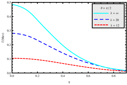
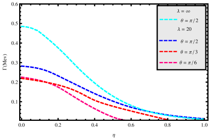
Figure 7: The thermal width versus the rapidity with finite coupling corrections. In this figure $\lambda={\infty}$ means that we have not considered any correction in the theory. Left: From top to down $\lambda=\infty,20,12$ and $\theta=\pi/2$. Right: From top to down for each curve, we assume $(\lambda=\infty,\theta=\pi/2)$, $(\lambda=20,\theta=\pi/2)$,$(\lambda=20,\theta=\pi/3)$, $(\lambda=20,\theta=\pi/6)$.

  

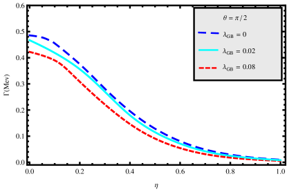
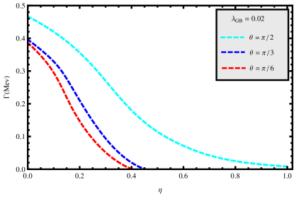
Figure 8: The thermal width versus the rapidity by considering the Gauss$-$Bonnet corrections. In the left plot, we fixed the angle as $(\theta=\pi/2)$ and from top to down $\lambda_{GB}$= 0, 0.02, 0.08. In the right plot we fixed the Gauss$-$Bonnet coupling $\lambda_{GB}=0.02$ and change the angle from top to down as $(\theta=\pi/2,\pi/3,\pi/6)$.

4.2 Thermal width at finite coupling

Now we plot the thermal width in the presence of $\mathcal{R}^{4}$ and Gauss$-$Bonnet corrections in Fig. 7 and Fig. 8, respectively. In Fig. 7, we plotted the thermal width versus the rapidity with the finite coupling corrections. In this figure, $\lambda={\infty}$ means that we have not considered any correction in the theory. By turning on the corrections, $\lambda$ decreases and the width also reduces. We have considered different angles for moving quarkonium to the wind in the right plot. One confirms that decreasing angle leads to decreasing the width. In Fig. 8, we considered Gauss$-$Bonnet quadratic curvature corrections to the AdS geometry. We fixed the angle $(\theta=\pi/2)$ and the Gauss$-$Bonnet coupling $(\lambda_{GB}=0.02)$ in the left and right plot, respectively. As it is clear, in the left plot from top to down $\lambda_{GB}$= 0, 0.02, 0.08 and in the right plot from top to down $(\theta=\pi/2,\pi/3,\pi/6)$. One concludes that at small rapidity decreasing coupling ($\lambda$ or $\lambda_{GB}$) leads to decreasing thermal width. More decreasing occurs in the case of $\mathcal{R}^{4}$ corrections. Thus one finds that the thermal width of static and moving quarkonium decreasing with considering the higher derivative corrections.

5 Conclusion

The main mechanism responsible for the suppression of quarkoniums is proposed to be color screening [2]. Recent studies show a more important reason than screening, which is the existence of an imaginary part of the potential. In this paper, we studied the effects of finite ’t Hooft coupling corrections on the imaginary potential and the thermal width of a moving heavy quarkonium from holography. An understanding of how these quantities change by these corrections may be essential for theoretical predictions in perturbative QCD [44, 7].

We discussed the limitations to the calculations of the imaginary potential and the thermal width in our method. It was explained that the valid region of the quark$-$antiquark distance for the onset of the imaginary part of the potential depends on the velocity of quarkonium. Also two different approaches for finding the thermal width have been studied in Fig. 6. Regarding the poor assumption in the case of approximate solution, we followed the exact solution to compute the width. As a result, one may conclude that the width vanishes for larger velocities of quarkonium.

Comparing with the static quarkonium [19], we find qualitatively the same results by considering higher derivative corrections. Briefly, in the presence of higher derivative corrections the following is found.

• The absolute value of the imaginary part of the potential of a moving or static heavy quarkonium becomes smaller.

• The thermal width of static or moving quarkonium decreasing with considering the higher derivative corrections.

Our results for the thermal width is similar to analogous calculations in perturbative QCD . It was argued that at strong coupling for a quarkonium with a very heavy constituent mass, the thermal width can be ignored [3, 45] which is in good agreement with our result. It is also interesting that in the ultra relativistic limit such corrections are not so important. It has been shown also that Gauss$-$Bonnet corrections can increase the nuclear modification factor $R_{AA}$, which leads decreasing the width [33, 34]. We found the same result, i.e. by considering the corrections the thermal width becomes effectively smaller.

Including other phenomenological parameters controlling the plasma properties would be interesting. It will be also very interesting to investigate the thermal width of a quarkonia in more realistic holographic backgrounds, such as in [46] and [47].

References

- [1] M. Laine, News on hadrons in a hot medium. arXiv:1108.5965 [hep-ph].
- [2] T. Matsui, H. Satz, J/psi Suppression by Quark-Gluon Plasma Formation. Phys. Lett. B 178 (1986) 416.
- [3] M. Laine, O. Philipsen, P. Romatschke, M. Tassler, Real-time static potential in hot QCD. JHEP 03 (2007) 054, arXiv:hep-ph/0611300.
- [4] M. A. Escobedo, The relation between cross-section, decay width and imaginary potential of heavy quarkonium in a quark-gluon plasma. J. Phys. Conf. Ser. 503 (2014) 012026 [arXiv:1401.4892 [hep-ph]].
- [5] N. Brambilla, J. Ghiglieri, A. Vairo, P. Petreczky, Static quarkantiquark pairs at finite temperature. Phys. Rev. D 78 (2008) 014017 [arXiv:0804.0993 [hep-ph]].
- [6] N. Brambilla, M. A. Escobedo, J. Ghiglieri, J. Soto, A. Vairo, Heavy Quarkonium in a weakly-coupled quark-gluon plasma below the melting temperature. JHEP 1009 (2010) 038 [arXiv:1007.4156 [hep-ph]].
- [7] N. Brambilla, M. A. Escobedo, J. Ghiglieri, A. Vairo, Thermal width and gluo-dissociation of quarkonium in pNRQCD. JHEP 1112 (2011) 116 [arXiv:1109.5826 [hep-ph]].
- [8] A. Dumitru, Quarkonium in a non-ideal hot QCD Plasma. Prog. Theor. Phys. Suppl. 187 (2011) 87 [arXiv:1010.5218 [hep-ph]].
- [9] A. Rothkopf, T. Hatsuda, S. Sasaki, Complex Heavy-Quark Potential at Finite Temperature from Lattice QCD. Phys. Rev. Lett. 108 (2012) 162001 [arXiv:1108.1579 [hep-lat]].
- [10] M. Margotta, K. McCarty, C. McGahan, M. Strickland, D. Yager-Elorriaga, Quarkonium states in a complex-valued potential. Phys. Rev. D 83 (2011) 105019 [Erratum-ibid. D 84 (2011) 069902] [arXiv:1101.4651 [hep-ph]].
- [11] B. Z. Kopeliovich, I. K. Potashnikova, I. Schmidt, M. Siddikov, Survival of charmonia in a hot environment. arXiv:1409.5147 [hep-ph].
- [12] F. Nendzig, G. Wolschin, Bottomium suppression in PbPb collisions at LHC energies. J. Phys. G 41 (2014) 095003 [arXiv:1406.5103 [hep-ph]].
- [13] T. Song, Y. Park, S. H. Lee, C. Y. Wong, The Thermal width of heavy quarkonia moving in quark gluon plasma. Phys. Lett. B 659 (2008) 621 [arXiv:0709.0794 [hep-ph]].
- [14] M. A. Escobedo, F. Giannuzzi, M. Mannarelli, J. Soto, Heavy Quarkonium moving in a Quark-Gluon Plasma. Phys. Rev. D 87 (2013) 11, 114005 [arXiv:1304.4087 [hep-ph]].
- [15] J. Casalderrey-Solana, H. Liu, D. Mateos, K. Rajagopal, U. A. Wiedemann, Gauge/string duality, hot QCD and heavy ion collisions. arXiv:1101.0618 [hep-th].
- [16] O. DeWolfe, S. S. Gubser, C. Rosen, D. Teaney, Heavy ions and string theory. arXiv:1304.7794 [hep-th].
- [17] E. Witten, Anti-de Sitter space and holography. Adv. Theor. Math. Phys. 2 (1998) 253 [arXiv:hep-th/9802150].
- [18] E. Witten, Anti-de Sitter space, thermal phase transition, and confinement in gauge theories. Adv. Theor. Math. Phys. 2 (1998) 505 [arXiv:hep-th/9803131].
- [19] K. B. Fadafan and S. K. Tabatabaei, Thermal width of quarkonium from holography. Eur. Phys. J. C 74 (2014) 2842 [arXiv:1308.3971 [hep-th]].
- [20] J. Noronha, A. Dumitru, Thermal width of the at large t’ Hooft coupling. Phys. Rev. Lett. 103 (2009) 152304 [arXiv:0907.3062 [hep-ph]].
- [21] S. I. Finazzo, J. Noronha, Estimates for the thermal width of heavy quarkonia in strongly coupled plasmas from holography. arXiv:1306.2613 [hep-ph].
- [22] J. L. Albacete, Y. V. Kovchegov, A. Taliotis, Heavy quark potential at finite temperature in AdS/CFT revisited. Phys. Rev. D 78 (2008) 115007 [arXiv:0807.4747 [hep-th]].
- [23] T. Hayata, K. Nawa, T. Hatsuda, Time-dependent heavyquark potential at finite temperature from gauge/gravity duality. arXiv:1211.4942 [hep-ph].
- [24] D. Giataganas, Observables in Strongly Coupled Anisotropic Theories. arXiv:1306.1404 [hep-th].
- [25] K. B. Fadafan, D. Giataganas and H. Soltanpanahi, The imaginary part of the static potential in strongly coupled anisotropic plasma. arXiv:1306.2929 [hep-th].
- [26] M. Ali-Akbari, Z. Rezaei, A. Vahedi, Thermal fluctuation and meson melting: holographic approach. arXiv:1406.2900 [hep-th].
- [27] J. Sadeghi, S. Tahery, The effects of deformation parameter on thermal witdth of moving quarqonia in plasma. arXiv:1412.8332 [hep-th].
- [28] M. Ali-Akbari, D. Giataganas, Z. Rezaei, Imaginary potential of heavy quarkonia moving in strongly coupled plasma. Phys. Rev. D 90 (2014) 8, 086001 [arXiv:1406.1994 [hep-th]].
- [29] S. I. Finazzo, J. Noronha, Thermal suppression of moving heavy quark pairs in strongly coupled plasma. arXiv:1406.2683 [hep-th].
- [30] K. B. Fadafan and E. Azimfard, On meson melting in the quark medium. Nucl. Phys. B 863 (2012) 347 [arXiv:1203.3942 [hep-th]].
- [31] J. Noronha, A. Dumitru, The heavy quark potential as a function of shear viscosity at strong coupling. Phys. Rev. D 80 (2009) 014007 [arXiv:0903.2804 [hep-ph]].
- [32] K. B. Fadafan, Heavy quarks in the presence of higher derivative corrections from AdS/CFT. Eur. Phys. J. C 71 (2011) 1799 [arXiv:1102.2289 [hep-th]].
- [33] A. Ficnar, S. S. Gubser, M. Gyulassy, Shooting string holography of jet qenching at RHIC and LHC. Phys. Lett. B 738 (2014) 464 [arXiv:1311.6160 [hep-ph]].
- [34] A. Ficnar, J. Noronha, M. Gyulassy, Falling strings and light quark jet quenching at LHC. Nucl. Phys. A 910-911 (2013) 252 [arXiv:1208.0305 [hep-ph]].
- [35] J. Pawelczyk, S. Theisen, AdS black hole metric at O(). JHEP 9809 (1998) 010, [hep-th/9808126];
- [36] T. Banks, M. B. Green, Non-perturbative effects in AdS(5) x S**5 string theory and d = 4 SUSY Yang-Mills. JHEP 9805, 002 (1998) [arXiv:hep-th/9804170];
- [37] S.S. Gubser, I.R. Klebanov, A.A. Tseytlin, Coupling constant dependence in the thermodynamics of supersymmetric Yang-Mills theory. Nucl. Phys. B534 (1998) 202, [hep-th/9805156];
- [38] R. G. Cai, GaussBonnet black holes in AdS spaces. Phys. Rev. D 65 (2002) 084014 [arXiv:hep-th/0109133].
- [39] S. Nojiri, S. D. Odintsov, Anti-de Sitter black hole thermodynamics in higher derivative gravity and new confining-deconfining phases in dual CFT. Phys. Lett. B 521 (2001) 87 [Erratum-ibid. B 542 (2002) 301] [arXiv:hep-th/0109122].
- [40] S. Nojiri, S. D. Odintsov, (Anti-) de Sitter black holes in higher derivative gravity and dual conformal field theories. Phys. Rev. D 66 (2002) 044012 [arXiv:hep-th/0204112].
- [41] M. Brigante, H. Liu, R. C. Myers, S. Shenker, S. Yaida, The viscosity bound and causality violation. arXiv:0802.3318 [hep-th]. A. Buchel, R. C. Myers, Causality of holographic hydrodynamics. JHEP 0908 (2009) 016 [arXiv:0906.2922 [hep-th]]. D. M. Hofman, Higher Derivative Gravity, Causality and Positivity of Energy in a UV complete QFT. Nucl. Phys. B 823 (2009) 174 [arXiv:0907.1625 [hep-th]].
- [42] D. Bak, A. Karch, L. G. Yaffe, Debye screening in strongly coupled N=4 supersymmetric YangMills plasma. JHEP 0708 (2007) 049 [arXiv:0705.0994 [hep-th]].
- [43] H. Liu, K. Rajagopal, U. A. Wiedemann, Wilson loops in heavy ion collisions and their calculation in AdS/CFT. JHEP 0703 (2007) 066 [hep-ph/0612168].
- [44] N. Brambilla, M. A. Escobedo, J. Ghiglieri, A. Vairo, Thermal width and quarkonium dissociation by inelastic parton scattering. JHEP 1305 (2013) 130 [arXiv:1303.6097 [hep-ph]].
- [45] M. Laine, Resummed perturbative estimate for the quarkonium spectral function in hot QCD. JHEP 05 (2007) 028, arXiv:0704.1720 [hep-ph].
- [46] U. Gursoy, E. Kiritsis, L. Mazzanti, F. Nitti, Deconfinement and Gluon Plasma Dynamics in Improved Holographic QCD,” Phys. Rev. Lett. 101 (2008) 181601 [27] S. S. Gubser, A. Nellore, S. S. Pufu and F. D. Rocha, Thermodynamics and bulk viscosity of approximate black hole duals to finite temperature quantum chromodynamics. Phys. Rev. Lett. 101 (2008) 131601
- [47] B. -H. Lee, S. Mamedov, S. Nam, C. Park, Holographic meson mass splitting in the Nuclear Matter. JHEP 1308 (2013) 045 [arXiv:1305.7281 [hep-th]].