Monetary Policy and Dark Corners in a stylized Agent-Based Model

Abstract

We extend in a minimal way the stylized macroeconomic Agent-Based model introduced in our previous paper Tipping , with the aim of investigating the role and efficacy of monetary policy of a ‘Central Bank’ that sets the interest rate such as to steer the economy towards a prescribed inflation and employment level. Our major finding is that provided its policy is not too aggressive (in a sense detailed in the paper) the Central Bank is successful in achieving its goals. However, the existence of different equilibrium states of the economy, separated by phase boundaries (or “dark corners”), can cause the monetary policy itself to trigger instabilities and be counter-productive. In other words, the Central Bank must navigate in a narrow window: too little is not enough, too much leads to instabilities and wildly oscillating economies. This conclusion strongly contrasts with the prediction of DSGE models.

I Introduction

The Agent Based Model (ABM) studied in this paper is a generalization of the “toy-ABM” (dubbed Mark-0) recently introduced in Tipping , following previous work by the group of Delli Gatti et al. DelliGatti . Mark-0 considers a stylized economy with firms and households, but no banks, no interest rates on loans and deposits, and therefore no direct concept of “monetary policy”. As discussed at length in Tipping , the original motivation of Mark-0 was mostly to illustrate the importance of phase diagrams and phase transitions in the context of ABMs, in particular the sensitivity of the state of the (artificial) economy on a subset of parameters. Small changes in the value of these parameters were indeed found to induce sharp variations in aggregate output, unemployment or inflation. In other words, endogenous crises can occur in such economies, as the result of insignificant or anecdotal changes in the environment. This possibility is quite interesting in itself, and must be contrasted with more traditional economic models, such as the popular DSGE framework DSGE ; Review , where the dynamics is linear and only large exogenous shocks can cause havoc. As recently pointed out by O. Blanchard in a very inspiring piece Blanchard : We in the field did think of the economy as roughly linear, constantly subject to different shocks, constantly fluctuating, but naturally returning to its steady state over time. […]. The main lesson of the crisis is that we were much closer to “dark corners” – situations in which the economy could badly malfunction – than we thought.

Because they can deal with non-linearities, heterogeneities and crises, ABMs are often promoted as possible alternatives to the DSGE models used in central banks as guides for monetary policy Eurace ; SantAnna ; Lagom ; Review . It is therefore clear that introducing interest rates monitored by a central bank in Mark-0 is mandatory for policy makers to develop any interest in the ABM research program in general and our model in particular. The aim of the present paper is to parsimoniously extend Mark-0 as to capture the effects of monetary policy on the course of the economy. We first identify and model several channels through which interest rates can feed into the behavior of firms and households. We then study different policy experiments, whereby the “Central Bank” attempts to reach a target inflation and/or unemployment level using a Taylor rule to set the interest rate (see Eq. (3) below). We find that provided the economy is far from phase boundaries (or “dark corners” Blanchard ) such policies can be successful, whereas too aggressive policies may in fact, unwillingly, drive the economy to an unstable state, where large swings of inflation and unemployment occur.

Our Agent-Based framework is voluntarily bare bones. It posits a minimal set of plausible ingredients that are most probably present in the real world in one form or the other. For example, we assume reasonable heuristic rules for the hiring/firing and wage policies of firms confronted with over- or under-production, or with a rising level of debt. Similarly, our model encodes in a schematic manner the consumption behavior of households facing inflation and rising rates, that is in fact similar to the standard Euler equation for consumption in general equilibrium/DSGE models DSGE . Our approach is therefore prone to the usual critique addressed to ABMs: the rules we implement are – although reasonable – to some degree arbitrary. The ABM community is of course aware of this weakness, with many attempts to resolve it, such as imposing consistency constraints on behavioral assumptions (see Dawid , Appendix A), or, even better, relying on micro-panel data that reveal how firms and households actually make decisions under different macro-economic or specific conditions (see for example Lein ; rates for the behavior of firms, and Souleles ; Ludvigson ; recession for the behaviour of households). However, reliable empirical data are still rather scarce and do not allow yet to answer all the questions needed to constrain and calibrate an ABM, even simple ones like Mark-0.

Our philosophy, explained in detail in Tipping , is different. We argue that the qualitative, aggregate behavior elicited by the Mark-0 model is in fact robust and generic, although the actual quantitative aspects may not be (as, for example, the precise value of the parameters of the Taylor rule beyond which instabilities occur). In other words, if one forgoes the idea of quantitatively predicting the macro-behaviour of the economy but is satisfied (at least temporarily) with a qualitative description of the possible aggregate behaviour, some progress is possible without detailed knowledge of the micro-rules. Our belief is backed by the idea – pervasive in many areas of science – that the aggregate properties of interacting entities can be classified in different phases, separated by phase boundaries across which radical changes of the emergent behavior take place. This idea has a long history, in particular in economics – remember, for example, the title of Thomas Schelling’s famous book: Micromotives and Macrobehaviour Schelling ; for more recent progress see e.g. Kirman ; Hommes ; Marsili ; Marsili2 ; Haldane ; Joao and for recent reviews: JPB ; Marsili-review . To bolster our belief that emergent aggregate properties are robust against micro-changes, we have tested many variants of the model presented below and indeed found that the overall behavior of our artificial economy is remarkably robust – in particular the presence of instabilities and crises. Following up on O. Blanchard’s lament Blanchard , the existence of large swaths of the parameter space where the economy is prone to violent crises seems to be an unavoidable fact that we have to learn to confront with Kirman ; Caballero .

The work presented in this paper is part of a growing literature of macroeconomic agent-based model testfatsion1 ; testfatsion2 . In the recent years several such models have been developed, allowing both to reproduce macro-stylized facts and to study policy design Dawid-review . Building upon SantAnna , Dosi et al. Dosi1 ; Dosi2 characterize the impact of fiscal and monetary policies on macroeconomics fluctuations. Fiscal policies are found to have a greater role in dampening business cycles, reducing unemployment and the likelihood of economic crises. Another example somewhat related to our work is Ref. Lengnick1 , which focuses on a simple ABM of financial markets coupled with a New Keynesian DSGE model, which allows one to reproduce endogenously stock price bubbles and business cycles and to study the introduction of financial taxes. Calibration and validation procedures have been explored in Haber ; Bianchi ; Fagiolo .

Although similar in spirit, the present study builds upon a slightly different perspective, following the framework and philosophy developed in Tipping . In particular, we model an idealized closed economy with linear production capabilities, no capital (labor is the only input for production), no innovation and growth, no financial sector, and only a minimal set of additional behavioural rules which couple the Central Bank monetary policy to firms’ and agents’ choices. In this sense, our model is much more parsimonious than what is found in the recent ABM literature and voluntarily overlooks important actors and processes at play in the real world. Our central concern is instead to characterize the qualitative behaviour of the emerging economy and investigate its dynamical stability with respect to the Central Bank’s policy.

The outline of the paper is as follows. In Section II we give a brief description of the Mark-0 model proposed in Tipping and detail the minimal additional rules we need to couple the monetary policy with firms’ and agents’ decisions. In Section III, we investigate the “natural” state of our toy-economy, in the presence of interest rates but without any Central Bank intervention. In Section IV, we perform several policy experiments: an expansionary monetary shock, and the implementation of a Taylor-rule monitoring of the interest rate by the Central Bank to achieve given employement and inflation targets. We establish the phase diagram of our model in the presence of this Taylor-rule based intervention. We briefly compare our findings to the prediction of DSGE models. We conclude in Section V. Appendix A gives further details about Mark-0; Appendix B investigates the continuous phase transition induced by the wary behaviour of indebted firms; finally, Appendix C gives a full pseudo-code of our model that should allow easy duplication of our results.

II Description of the model

II.1 Brief summary of the minimal “Mark-0” model

The Mark-0 closed economy is made of firms and households. While the latter sector is represented at an aggregate level, firms are heterogeneous and treated individually. Each firm $i=1,\dots,N_{F}$ at time $t$ produces a quantity $Y_{i}(t)$ of perishable goods that it attempts to sell at price $p_{i}(t)$. It needs a number of $N_{i}(t)=Y_{i}(t)/\zeta_{i}$ of employees to produce $Y_{i}(t)$, and pays a wage $W_{i}(t)$. The demand $D_{i}$ for good $i$ depends on the global consumption budget of households $C_{B}(t)$, itself determined as a fraction of the household savings (that include the last wages), and it is a decreasing function of the asked price $p_{i}(t)$, with a price sensitivity parameter that can be tuned – see Appendix A.

To update their production, price and wage policy, firms use reasonable “rules of thumb” Tipping that we detail in Appendix A and that were already (partly) justified in the original work of Delli Gatti et al. DelliGatti . For example, production is decreased and employees are made redundant whenever $Y_{i}>D_{i}$, and vice-versa. The adjustment speed can however be asymmetric, i.e. the ratio $R$ of hiring adjustement speed to firing adjustement speed is not necessarily equal to one, for example because of labour laws. This turns out to be one of the most important control parameter that determines the fate of the overall economy.

In the initial state of the economy, firms are heterogenous in size and prices (with a uniform distribution around the average size and price, see Appendix C for details), but all offer the same wage and see the same demand. This is arbitrary and of little importance, because the stationary state of the model is statistically independent of the initialization.

When the Mark-0 economy is set in motion, it soon becomes clear that some firms have to take up loans in order to stay in business. One therefore immediately has to add further rules for this to take place. In the zero-interest rate world of Mark-0, we let firms freely accumulate a total debt up to a threshold that is a multiple $\Theta$ of total payroll, beyond which the firm is declared bankrupt (its debt is then repaid partly by households and partly by surviving firms, such that there is no net creation of money). From this point of view the parameter $\Theta$ determines the maximum credit supply available to firms. Fixing the value of $\Theta$ plays the role of a primitive monetary policy, since the total amount of money circulating in the economy (‘broad money’) directly depends on $\Theta$ Tipping . When $\Theta=0$, no debt is allowed (zero leverage), while when $\Theta\rightarrow\infty$, firms have not limit on the loans they need to continue business (unbounded leverage).

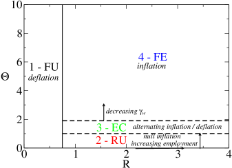
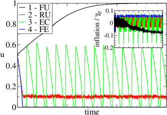
Figure 1: (Left) Phase diagram in the $R-\Theta$ plane of the basic Mark-0 model as obtained in Tipping with wage update. There are four distinct phases separated by critical lines. The Full Employment (FE) phase ($R>R_{c}$, $\Theta$ large) is characterized by positive average inflation, while there is deflation in the Full Unemployment (FU) phase ($R<R_{c}$). Endogenous Crises (EC) are characterized by alternating cycles of inflation and deflation, and occur for $R>R_{c}$, $\Theta$ intermediate. Finally, $R>R_{c}$, small $\Theta$ correspond to a region of small inflation and Residual Unemployment (RU). The location of phase boundaries is only weakly affected by the choice of the other parameters of Mark-0, see Tipping . (Right) Typical trajectories of the unemployment rate $u(t)$ for each of the phases. In the inset, the price variations are shown, displaying either inflation (in the FE phase) or deflation (in the FU phase). $\gamma_{p}^{-1}$ (resp. $\gamma_{w}^{-1}$) sets the characteristic time scale for price adjustments (resp. wages) in the model, see Appendix A. The surprising occurrence of endogenous oscillations in the EC phase can be fully understood analytically, see Synchro .

While there are several other parameters needed to define completely Mark-0 (9 parameters in total, see Appendix A), the detailed investigation of Tipping has established that only $R$ and $\Theta$ are the ones determining the phase-diagram of the model, shown in Fig. 1, where we also plot typical trajectories of the economy in each phase. It is important to stress that this diagram is extremely robust against both details of the model specification and the value of the other parameters, which only affect the above phenomenology quantitatively, but leave the qualitative emergent behavior essentially unchanged. Its salient features are Tipping :

• When $\Theta=\infty$ the economy is characterized by two distinct phases separated by a first order (discontinuous) phase transition as a function of the parameter $R$. When $R<R_{c}$ (i.e. fast downward production adjustments), one finds at long times a collapse of the economy towards a deflationary/low demand/full unemployment state (FU). For $R>R_{c}$, on the other hand, the long run state of the economy is characterized by a positive inflation/high demand/full employment phase (FE).

• When $\Theta<\infty$ the above description holds but must be refined to allow for the appearance of three sub-phases for $R>R_{c}$:

  1. a full employment and inflationary phase for high values of $\Theta$ (the FE phase, similar to the $\Theta=\infty$ case);

  2. a phase for intermediate values of $\Theta$ characterized by high employment and inflation on average, which is, however, intermittently disrupted by “endogenous crises” (EC), that temporarily bring deflation and high unemployment spikes;

  3. a phase with zero inflation and residual unemployment for small $\Theta$ (the RU phase), where the impossibility to obtain loans creates a positive stationary level of bankruptcies.

Note that the unexpected occurrence of purely endogenous oscillations in the EC phase can in fact be understood fully analytically Synchro and it is a robust feature that only relies on very mild assumptions about the destabilizing feedback mechanisms present in the economy.

II.2 Introducing interest rates in Mark-0

We now introduce in the model a banking system made up of a Central Bank (CB) which sets the base interest rate $\rho_{0}(t)$ (and, as part of a prudential policy, the parameter $\Theta$ that controls the maximum credit supply available to firms), and a private banking system that will act as a transmission belt for the CB policy, by setting interest rates on deposits ($\rho^{\text{d}}(t)$) and on loans ($\rho^{\ell}(t)$). These interest rates will in turn impact the economy through three channels that we detail below: a) direct cost of loans and gains on deposits; b) behavior of the firms; c) behavior of households.

II.2.1 The Central Bank policy

The CB attempts to steer the economy towards a target inflation level $\pi^{*}$ and employment level $\varepsilon^{*}$ (equivalent to a target output, since the productivity $\zeta$ is set to unity in the present version of the model). The instantaneous inflation $\pi(t)$ and employment level $\varepsilon(t)$ are defined here as:

$$\pi(t)=\frac{\overline{p}(t)-\overline{p}(t-1)}{\overline{p}(t-1)};\qquad\overline{p}(t)=\frac{\sum_{i}p_{i}(t)Y_{i}(t)}{\sum_{i}Y_{i}(t)},$$ (1)

where $\overline{p}(t)$ is the production-weighted average price, and:

$$\varepsilon(t)=\frac{1}{N}\sum_{i}Y_{i}(t)\ ,\qquad u(t)=1-\varepsilon(t),$$ (2)

where $N$ is the total workforce, and $\varepsilon(t),u(t)$ are respectively the employment and unemployment rate.

We will assume that the monetary policy followed by the CB for fixing the base interest rate is described by a standard Taylor rule of the form Mankiw ; DSGE :

$$\rho_{0}(t)=\max\left(\rho^{*}+10\ \phi_{\pi}[\widetilde{\pi}(t)-{\pi}^{*}]+\phi_{\varepsilon}\log{[\widetilde{\varepsilon}(t)/\widehat{\varepsilon}^{*}]},\,0\right)$$ (3)

where $\rho^{*}$ is the “natural” interest rate that would prevail if the target inflation ${\pi}^{*}$ and target employment $\varepsilon^{*}$ were reached, and $\alpha_{\pi,\varepsilon}>0$ quantify the intensity of the policy (high values of the parameters correspond to aggressive policies). Note that $\rho_{0}$ is constrained to be non-negative. The factor $10$ in front of $\phi_{\pi}$ is only there for convenience, such that interesting values of $\phi_{\pi}$ and $\phi_{\varepsilon}$ are of the same order of magnitude. The notation $\widetilde{x}(t)$ corresponds to the exponential moving average of the variable $x(t)$, defined as:

$$\widetilde{x}(t+1)=\omega x(t)+(1-\omega)\widetilde{x}(t).$$ (4)

In order to avoid unnecessary excessive policy response when the target employment rate is too far from the actual employment rate, we actually define a one-time-step target employment rate $\widehat{\varepsilon}^{*}$ as

$$\widehat{\varepsilon}^{*}=\min{\{1.025\ \widetilde{\varepsilon}(t),{\varepsilon}^{*}\}}$$ (5)

meaning that if the employment rate is much lower than the policy target ${\varepsilon}^{*}$ the CB will try to increase it by $2.5\%$ at each time step until the target is reached. Such a regularization was found not to be needed for inflation.

II.2.2 The banking sector

Households in the Mark-0 economy cannot borrow and are thus characterized by their total savings $S(t)\geq 0$. Firms, on the other hand, can have either deposits (${\cal E}_{i}>0$) or liabilities (${\cal E}_{i}<0$). Defining ${\cal E}^{+}=\sum_{i}\max{({\cal E}_{i},0)}$ and ${\cal E}^{-}=-\sum_{i}\min{({\cal E}_{i},0)}$, the balance sheet of the banking system reads:

$$M+{\cal E}^{-}(t)=S(t)+{\cal E}^{+}(t)\equiv\mathcal{X}(t),$$ (6)

where $M$ is the amount of currency (or initial deposits) created by the central bank, which is kept fixed in time, and $\mathcal{X}$ is the total amount of deposits, therefore to initial deposits $M$ plus the money created by the banking system when issuing loans.

We now assume that the banking sector fixes the interest rates on deposits and loans ($\rho^{\text{d}}(t)$ and $\rho^{\ell}(t)$ respectively) uniformly for all lenders and borrowers according to the following rules:

$$\rho^{\ell}(t) = \rho_{0}(t)+f\frac{{\cal D}(t)}{{\cal E}^{-}(t)}$$

$$\rho^{\text{d}}(t) = \frac{\rho_{0}(t){\cal E}^{-}(t)-(1-f){\cal D}(t)}{{\cal X}(t)}\ .$$ (7)

where ${\cal D}(t)$ is the aggregate costs coming from all firms that just defaulted, bearing on the banking sector. Note that $\rho^{\text{d}}\leq\rho_{0}\leq\rho^{\ell}$. The parameter $f\in[0,1]$ reflects the impact of these defaults – either entirely on the cost of loans ($f=1$) or on the revenue of deposits ($f=0$). The logic behind rule Eq. (II.2.2) is that the interest rate on loan increases when defaults increase, while the rate on deposits is chosen in such a way that the profits of the banking sector are exactly zero at each time step. Indeed, one has, for any value of $f$:

$$\underbrace{\rho^{\ell}(t){\cal E}^{-}(t)}_{\text{interest from loans}}\quad-\underbrace{\rho^{\text{d}}(t){\cal X}(t)}_{\text{interest paid on deposits}}\quad-\underbrace{{\cal D}(t)}_{\text{cost of defaults}}\equiv\,0.$$ (8)

Note that $\rho^{\text{d}}(t)$ can become negative for large enough ${\cal D}(t)$ when $f\neq 1$, i.e. the deposits are taxed by the banking sector. This could be interpreted as a kind of “bail-in tax” to absorb debt in extreme cases. In our simulations where $f=0.5$, this situation does occur in the unstable phases of the economy during a relatively short fraction of the time, corresponding to the peaks of the unemployment spikes. Finally, one could introduce an extra haircut in $\rho^{\ell}$ or $\rho^{\text{d}}$ if one wants to model a profit-seeking banking sector, but the resulting profits would somehow have to be re-injected in the economy – an extra modeling step that we avoid at this stage by assuming the above no-profit rule.

II.2.3 Households’ consumption budget

As mentioned above, one major simplification of Mark-0 is to treat the whole household sector at the aggregate level, and to represent it with only a few variables: total savings $S(t)$, total wages $W_{T}(t)=\sum_{i}W_{i}(t)Y_{i}(t)$, and total consumption budget $C_{B}(t)$ (which, as emphasized in Tipping , is in general larger than the actual consumption $C(t)$).

The effect of interest rates on households is two-fold. First, quite trivially, they receive some interest on their savings $S(t)$ that adds to the wages $W_{T}(t)$ and dividends as their total income. Second, the comparison between interest rates and inflation creates an incentive to consume or to save. This is in the spirit of the standard Euler equation of DSGE models where consumption is found to depend on the difference of rates on deposits $\rho^{\text{d}}(t)$ and inflation $\pi(t)$ (see e.g. Mankiw ; DSGE ). We therefore posit that the consumption budget of households $C_{B}(t)$ is given by:

$$C_{B}(t)=c(t)\left[S(t)+W_{T}(t)+\rho^{\text{d}}(t)S(t)\right]\quad\text{with}\quad c(t)=c_{0}\left[1+\alpha_{c}(\widetilde{\pi}_{t}-\widetilde{\rho}^{\text{d}}_{t})\right],$$ (9)

where $c(t)\in[0,1]$ is the consumption propensity (taken to be a constant in Mark-0) and $\alpha_{c}>0$ is a coupling constant that determines the sensitivity of households to the (moving average of the) difference between inflation and the interest paid on their savings. The larger the difference between the two, the larger the propensity to consume, as in standard equilibrium models Mankiw , but with here undetermined phenomenological parameters $c_{0},\alpha_{c}$ that should in principle be measured on micro-data (surveys, laboratory experiments, etc., see e.g. Souleles ; Ludvigson ; recession ).

Apart from these changes, the behavior of households is exactly the same as in Mark-0, see Tipping and Appendix A for details.

II.2.4 Firms’ policy when debt is costly

Financial fragility.

Unlike households the $N_{\rm F}$ firms are heterogeneous and treated individually. Each firm is characterized by its production $Y_{i}$ (equal to its workforce), demand for its goods $D_{i}$, price $p_{i}$, wage $W_{i}$ and cash balance ${\cal E}_{i}$. The debt level of a firm is measured through the ratio

$$\Phi_{i}=-{\cal E}_{i}/(W_{i}Y_{i}),$$ (10)

which we interpret as an index of financial fragility. If $\Phi_{i}(t)<\Theta$, i.e. when the flux of credit needed from the bank is not too high compared to the size of the company (measured as the total payroll), the firm is allowed to continue its activity. If on the other hand $\Phi_{i}(t)\geq\Theta$, the firm defaults and contributes to total default costs ${\cal D}(t)$.

Production and wage update.

If the firm is allowed to continue its business, it adapts its price, wages and productions according to reasonable “rules of thumb” introduced in Tipping – see Appendix A. In particular, the production update is chosen as:

$$\begin{split}\text{If }Y_{i}(t)<D_{i}(t)&\hskip 10.0pt\Rightarrow\hskip 10.0ptY_{i}(t+1)=Y_{i}(t)+\min\{\eta^{+}_{i}(D_{i}(t)-Y_{i}(t)),u^{*}_{i}(t)\}\\ \text{If }Y_{i}(t)>D_{i}(t)&\hskip 10.0pt\Rightarrow\hskip 10.0ptY_{i}(t+1)=Y_{i}(t)-\eta^{-}_{i}[Y_{i}(t)-D_{i}(t)]\\ \end{split}$$ (11)

where $u^{*}_{i}(t)$ is the maximum number of unemployed workers available to the firm $i$ at time $t$ (see Appendix A). The coefficients $\eta^{\pm}\in[0,1]$ express the sensitivity of the firm’s target production to excess demand/supply, and they were constant in Mark-0.

Here, we further postulate that the production adjustment depends on the financial fragility $\Phi_{i}$ of the firm. Firms that are close to bankruptcy are arguably faster to fire and slower to hire, and vice-versa for healthy firms. In order to model this tendency, we posit that the coefficients $\eta^{\pm}_{i}$ for firm $i$ are given by:

$$\eta^{-}_{i}=\eta_{0}\max(1+\Gamma\Phi_{i}(t),0)$$

$$\eta^{+}_{i}=R\eta_{0}\max(1-\Gamma\Phi_{i}(t),0)$$ (12)

where $\eta_{0}$ is a fixed coefficient, identical for all firms, and $R$ is the propensity ratio discussed in the previous section. The factor $\Gamma>0$ measures how the financial fragility of firms influences their hiring/firing policy, since a larger value of $\Phi_{i}$ then leads to a faster downward adjustment of the workforce when the firm is over-producing, and a slower (more cautious) upward adjustment when the firm is under-producing. The above definition however ensures that $\eta^{\pm}$ always remain non-negative, i.e. the reaction of the firms is always in the intuitive direction.

It is plausible that the financial fragility of the firm also affects its wage policy: we give in Appendix A the wage update rules of Mark-0 and their modification to account for financial fragility, through the very same parameter $\Gamma$. In essence, deeply indebted firms seek to reduce wages more rapidly, whereas flourishing firms tend to increase wages quickly.

The baseline Mark-0 model corresponds to $\Gamma\equiv 0$, and leads to the phase diagram shown in Fig. 1 above. Interestingly, a non-zero value of $\Gamma=\Gamma_{0}$ (constant across firms and in time) changes substantially the nature – but not the existence – of the phase transition between the full employment (FE) and full unemployment (FU) phase. The first order (discontinuous) transition for $\Gamma_{0}=0$, $\Theta=\infty$ found in Tipping and shown in Fig. 1, is replaced by a second order (continuous) transition when the firms adapt their behavior as a function of their financial fragility, i.e. when $\Gamma_{0}>0$. Moreover, the “bad” FU phase for $R<R_{c}$ becomes a partial unemployment phase with $u<1$ that continuously varies with $R$: see Appendix B and Fig. 9 for full details. As firms become more careful, employment can be to some extent preserved – as expected.

The “good” phase of the economy, on the other hand, is only mildly affected by a non zero $\Gamma_{0}$ – for example the FE region of Fig. 1 expands downwards, which is expected since firms manage more carefully their balance sheet, reducing the occurrence of defaults.

The influence of interest rates on the strategy of firms.

We now argue that $\Gamma$ should in fact depend on the difference between the interest rate and the inflation: high cost of credit makes firms particularly wary of going into debt and their sensitivity to their financial fragility should be increased. Therefore, we postulate that interest rates feedback into the behavior of the firm primarily through the $\Gamma$ parameter, that we model in the simplest possible way as:

$$\Gamma=\max{\{\alpha_{\Gamma}(\widetilde{\rho}^{\ell}(t)-\widetilde{\pi}(t)),\Gamma_{0}\}},$$ (13)

where $\alpha_{\Gamma}$ (similarly to $\alpha_{c}$ above) captures the influence of the real interest rate $\widetilde{\rho}^{\ell}(t)-\widetilde{\pi}(t)$ on the hiring/firing policy of the firms. Whenever the real interest rate stays below $\Gamma_{0}/\alpha_{\Gamma}$, the response of firms to changes of interest rates is negligible (perhaps as reported in rates ), whereas larger rates lead to a substantial change in the firms policy. The case $\alpha_{\Gamma}=0$ but $\Gamma_{0}>0$ corresponds to the above discussion and it is interesting in itself (see Appendix B). However, since we will be mostly concerned with policy issues, we will concentrate below on the other extreme case, $\alpha_{\Gamma}>0$ and $\Gamma_{0}=0$, keeping in mind that reality is probably in-between. Note that $\Gamma$ as defined above is now zero when real interest rates are negative, and is positive otherwise.

II.3 Summary

II.3.1 How many new assumptions?

In our attempt to include interest rates and monetary policy into the Mark-0 framework, we have made new behavioral assumptions, that we tried to keep as simple and as parsimonious as possible:

• For the Central Bank, we have merely adapted the standard Taylor rule to our setting, introducing three monetary policy parameters $\rho^{*}$ (the natural interest rate) and $\phi_{\pi},\phi_{\varepsilon}$ (the Taylor rule parameters), and two targets: inflation $\pi^{*}$ and employment $\varepsilon^{*}$.

• For the banking sector, we have essentially used trivial accounting rules to ensure a no-profit condition on loans and deposits. The only new parameter is $f$ and determines how much of the cost of bankruptcy must be paid by loans or by deposits. However, this parameter plays very little role in the qualitative behaviour of the economy, so we set it to $f=1/2$ henceforth.

• For the households, we assume an Euler-like behaviour of the consumption budget as a function of the real interest rate on deposits, i.e. the consumption budget decreases when the real rate is high and increases when it is low, with a slope given by parameter $\alpha_{c}$.

• For the firms, the hiring/firing and wage policy is affected by the real rate on loans. When it is high, indebted firms are more careful, firing more rapidly and hiring less. The unique parameter coupling the real interest rate to the firms policy is $\alpha_{\Gamma}$.

These last two additional rules are to some extent arbitrary. However, they capture effects that certainly exist in the real world; furthermore changing the detailed implementation we chose here while keeping the spirit of these rules lead to very similar conclusions. This is in line with our general claim that macro-behaviour is to a large degree insensitive to micro-rules.

In summary, we want to emphasize that our extension of Mark-0 is very parsimonious: we have only added two behavioral parameters ($\alpha_{c},\alpha_{\Gamma}$).

II.3.2 Recovering Mark-0

From the above discussion, we see that the core Mark-0 model of Tipping is recovered whenever the baseline interest rate is zero $\rho^{*}=0$, the CB is inactive ($\phi_{\pi}=\phi_{\varepsilon}=0$), and households and firms are insensitive to interest rates and inflation (i.e. setting $\alpha_{c}=\alpha_{\Gamma}=0$).

There is however a slight remaining difference with Mark-0 in the resolution of bankruptcies. The closest one can get is by setting $f=0$, i.e. absorbing default costs only through savings. In this case the only non-zero interest rate remaining in the dynamics of the model is the one on deposits, which is negative: $\rho^{\text{d}}=-{{\cal D}(t)}/{{\cal X}(t)}\leq 0$. This indeed roughly corresponds to the default resolution described in Tipping where default costs are paid by households and firms savings. There are also minor differences in the time-line of the model (in particular bankruptcies are resolved before price, production and wages are updated). All these differences however have a negligible quantitative impact on the results below.

III The “natural” behavior of the economy (without monetary policy)

In this section we analyze the features of the model that arise from the introduction of interest rates in the Mark-0 economy, disregarding for a while any active monetary policy (i.e. setting $\phi_{\pi}=\phi_{\varepsilon}\equiv 0$ in Eq. (3) above). In other words, we study an economy where the baseline interest rate is equal to $\rho^{*}$, constant in time, and affects both the consumption propensity of households through the parameter $\alpha_{c}$ appearing in Eq. (9), and the firms hiring/firing propensity through the parameter $\alpha_{\Gamma}$ appearing in Eq. (13), with $\Gamma_{0}=0$ henceforth.

When interest rates do not feedback at all into firms’ and agents’ behavior (i.e. for $\alpha_{\Gamma}=\Gamma_{0}=0$ and $\alpha_{c}=0$) the phenomenology of the Mark-0 model is basically unaffected; in particular the phase diagram Fig. 1 is unchanged.

III.1 Coupling between interest rates and firms behavior

When $\alpha_{\Gamma}>0$, on the other hand, the overall behavior of the economy evolves as expected: as long as $\rho^{*}$ is less than the inflation rate, nothing much happens, in particular because Eq. (13) gives $\Gamma=\Gamma_{0}\equiv 0$ here. When $\rho^{*}$ exceeds the inflation rate, one observes that the unemployment rate $u$ starts increasing with $\rho^{*}$, while the demand for credit and the inflation rate itself nosedive as expected.

In Fig. 2 (left) we plot the phase diagram of the model in the $\rho^{*}-\Theta$ plane when $R=2>R_{c}$, and for a fixed value $\alpha_{\Gamma}=50$. For $\rho^{*}$ smaller than a certain value $\rho^{**}\approx 1.3$, one observes the familiar three phases FE-EC-RU as $\Theta$ is decreased, as in Fig. 1. However, for a baseline rate larger than $\rho^{**}$, the FE and EC phase disappear entirely, and the Residual Employment phase (with $u\sim 30\%$) prevails for all values of $\Theta$. To wit, when interest rates are too high, firms hesitate to accumulate more debt (even if they are allowed to when $\Theta$ is high). Rather, they prefer reducing their work force when needed, keeping the unemployement at a relatively high level.

Fig. 2 (right) allows one to understand the role of $\alpha_{\Gamma}$: there we show the phase diagram in the $\rho^{*}-\alpha_{\Gamma}$ plane for fixed values of $R=2$ and $\Theta=3$, such that the economy is in the Full Employment phase for $\alpha_{\Gamma}=0$. A sudden phase transition between the FE and RU phases occurs for a critical value $\rho^{**}(\alpha_{\Gamma})$; the larger the sensitivity to interest rates – i.e. the larger $\alpha_{\Gamma}$ – the smaller the critical value of the baseline interest rate beyond which the economy is destabilized. It is interesting (and quite counterintuitive) that the aggregate behavior of the economy is not a smooth function of the interest rate. When firms are risk averse and fear going into debt, large enough interest rates lead to more unemployment that spirals into a destabilizing feedback loop. This is one of the “dark corners” that ABMs can help uncovering.

III.2 Coupling between interest rates and household behavior

Perhaps unexpectedly, the coupling between interest rate and consumption (captured by parameter $\alpha_{c}$) appears to have much smaller influence on the “natural” state of the economy, at least when $\alpha_{c}$ is chosen within a reasonable range. Its main influence is to increase the output fluctuations around the steady state, by amplifying price trends through the resulting reduction/increase in consumption. Interestingly, we find that for $\Theta\gg 1$ and independently of $\rho^{*}$, $\alpha_{c}$ has a stabilising effect on the economy: $R_{c}$ shifts to lower values as $\alpha_{c}$ increases (in the absence of monetary policy). Clearly, micro-data is needed to estimate the value of $\alpha_{c}$ for realistic applications; but since this parameter plays a small role we will choose rather arbitrarily $\alpha_{c}=4$, unless explicitly stated. This corresponds to a moderate sensitivity to inflation/interest rates: a rise of the interest rate of $1\%$/year corresponds to a decrease of $4\%$ of the consumption propensity.

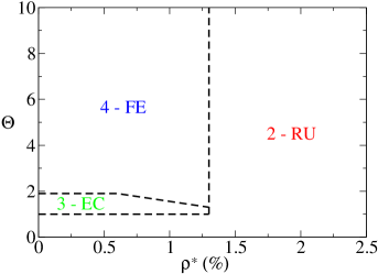
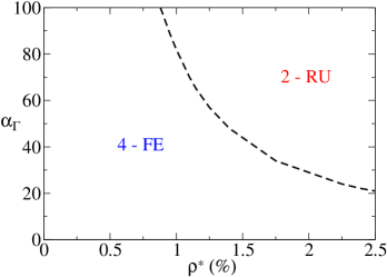
Figure 2: Left: Phase diagram of the “natural” state of the economy in the $\rho^{*}-\Theta$ plane (i.e. with no monetary policy, $\phi_{\varepsilon}=\phi_{\pi}=0$) when both firms’ and households’ decisions are sensitive to the rate level: $\alpha_{\Gamma}=50$ and $\alpha_{c}=4$. For small enough rates $\rho^{*}<\rho^{**}$, one recovers the FE-EC-RU phases as $\Theta$ is decreased. When $\rho^{*}>\rho^{**}$, however, the RU phase prevails for all values of $\Theta$, which becomes irrelevant. Right: Phase diagram in the $\rho^{*}-\alpha_{\Gamma}$ plane for $\Theta=3$, showing the dependence of the critical value $\rho^{**}$ on $\alpha_{\Gamma}$. The other parameters of the model are set to: $R=2$ (with $\eta^{0}_{-}=0.1$), $c_{0}=0.5$, $\Gamma_{0}=0$, $\varphi=0.1$, $\gamma_{p}=\gamma_{w}=0.05$, $\beta=2$, $\delta=0.02$, $f=0.5$, $N_{F}=2000$ (see Appendix A for a definition of all these parameters).

IV Monetary policy experiments

We now consider a simple policy framework where the Central Bank adjusts the base interest rate $\rho_{0}(t)$ in order to achieve its inflation and employment targets. Given the simplicity of our model we are mainly interested here in gaining a qualitative understanding of the possible consequence of a Taylor-rule based monetary policy in a stylized Agent-Based framework. We defer parameter calibration, detailed comparison with simple DSGE models and more quantitative insights to future studies.

Our major finding is that provided its policy is not too aggressive and the economy not too close to a phase transition, the CB is successful in steering the economy towards its targets. However, the mere presence of different equilibrium states of the economy separated by phase boundaries (i.e. “dark corners”) may deeply alter the impact of monetary policy. Indeed, we will exhibit cases where the monetary policy by itself triggers large instabilities and is counter-productive.

As in the previous section, we will refer to the state obtained without any response of the CB, i.e. when $\phi_{\pi}=\phi_{\varepsilon}=0$, as the “natural” state of the economy (for a given set of parameters). The corresponding “natural” value of a variable $x$ will be denoted by $x_{\text{nat}}$. In order to simplify the analysis and since most of the parameters of our model play little role in the qualitative behavior of the economy we set once and for all some of them to the values given in the caption of Fig. 2 and choose $\rho^{*}=2\%$. We only focus on the four parameters defining the CB policy (i.e. $\phi_{\pi},\ \phi_{\varepsilon},\ {\varepsilon}^{*}$ and ${\pi}^{*}$), the parameters of the transmission channels (i.e. $\alpha_{c}$ and $\alpha_{\Gamma}$), and the two parameters locating the system in the phase diagram of Fig. 1 (i.e. the hiring/firing ratio $R$ and the bankruptcy threshold $\Theta$).

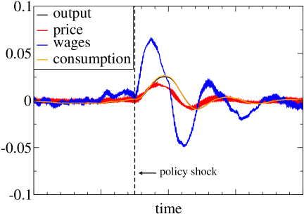
Figure 3: Aggregate response of the economy to a policy shock represented by a drop in the interest rate $\rho_{0}$ set by the central bank (from $2\%$ to $1.8\%$). The vertical dashed line gives the timing of the policy shock. All aggregate variables are represented as a relative variation from their average values prior to the shock. For a better visualization, we amplified by a factor $100$ the wage and price responses. Note that the damped oscillation relaxation towards equilibrium. Parameters are $\Theta=3$, $\rho^{*}=2\%$, $\alpha_{\Gamma}=50$, $\alpha_{c}=4$, and other parameters as in Fig. 2.

IV.1 A monetary shock

In order to check that our framework produces reasonable results, it is interesting to start with the simplest policy experiment, i.e. an expansionary monetary policy shock where the baseline interest rate is instantaneously decreased from $2\%$ to $1.8\%$, all other parameters of the model being fixed, and with no further intervention of the Central Bank (i.e. $\phi_{\pi}=\phi_{\varepsilon}=0$). The resulting dynamics of output, wages and prices is shown in Fig. 3 and can be compared with e.g. Fig 1 of Ref. Christiano . It is gratifying to see that our simple modelling strategy, in particular the way the monetary policy is channelled to the economy, does lead to a quite realistic shape of impulse response functions, at least qualitatively. In fact, the empirical hump-shaped response of the output reported in Christiano is quite well reproduced by their DSGE model with nominal rigidities. Although the underlying microfundations are very different, our ABM indeed includes frictions: all adjustments (of production, wages and prices) in our model are only made progressively. So our framework is indeed able to capture effects predicted by enhanced DSGE models. No attempt was made here to adjust parameters to quantitatively match empirical data, in particular the time scales: this is beyond the scope of the present study which is primarily intended to be a description of the qualitative behavior of our toy-economy.

IV.2 Mild vs aggressive monetary policy

In Fig. 4 for example, we show the result of the policy of the Central Bank that attempts to bring down the natural unemployment rate of $u_{\text{nat}}\approx 0.33$ (a rather large value corresponding to $\Theta=2$, $R=2$ and $\rho^{*}=2\%$) to a low target of $1-{\varepsilon}^{*}=u^{*}=0.05$. The target inflation is ${\pi}^{*}=0.2\%$ per time step (corresponding to $2.4\%$ annual if one interprets the time step to be a month), compared to a natural inflation that fluctuates around zero: $\pi_{\text{nat}}\approx 0$. The left graph corresponds to a mild monetary policy, with Taylor-rule parameters set to $\phi_{\pi}=\phi_{\varepsilon}=0.5$. The policy is seen to be rather successful: the inflation is on target, while unemployment goes down to $u\approx 0.07$, not far from the target of $0.05$. But now look at the graph on the right, where the only difference is the aggressiveness of the CB that attempts to reach target too quickly, merely doubling the value of $\phi_{\pi}=\phi_{\varepsilon}\rightarrow 1$. In this case, the monetary policy has induced strong instabilities, with “business cycles” of large amplitude and inflation all over the place.

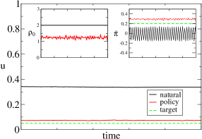
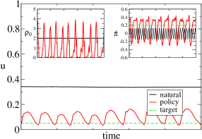
Figure 4: In these plots we select the same natural state of the economy with $\Theta=2$, $R=2$, $\rho^{*}=2\%$ and $\alpha_{\Gamma}=50$, such that $u_{\text{nat}}\approx 0.33$ and $\pi_{\text{nat}}\approx 0$ (but fluctuating). The CB sets a much lower unemployment target of $u^{*}=0.05$ and an inflation target of ${\pi}^{*}=0.2\%$. In the left plot the CB policy is moderate ($\phi_{\pi}=\phi_{\varepsilon}=0.5$) and basically achieves its goals, while in the right plot the policy is aggressive ($\phi_{\pi}=\phi_{\varepsilon}=1$) and destabilizes the whole economy. In the insets, $\rho_{0}$ and $\pi$ are given in $\%$s. The period of the business cycles in the right plot corresponds to $\approx 4$ years if the elementary time unit of the model is one month. Larger spikes of unemployment are also observed with much lower frequency (not shown).

We show in Fig. 5 the result of an extensive exploration of the role of $\phi_{\pi}$ and $\phi_{\varepsilon}$ when $\Theta=2$, $R=2$ and $\rho^{*}=2\%$. One sees that there is a wedge-like region around $\phi_{\pi}=\phi_{\varepsilon}=0$ where the policy does not induce instabilities (signaled by a yellow/orange hue in Fig. 5-right). However, the region of parameters where the unemployment rate is significantly reduced is only a subset of this wedge, corresponding to the black region in Fig. 5-left, where $\phi_{\varepsilon}\sim 0.5$, $\phi_{\pi}\leq 0.5$. In other words, the Central Bank must navigate in a narrow window: too little is not enough, too aggressive is counterproductive and leads to instabilities and wildly oscillating economies.

Fig. 5 also reveal that in our toy-world, a Central Bank with a dual mandate (inflation and output) enjoys a wider region of stability compared to a Central bank with inflation as the only mandate. Steering inflation and output simultaneously increases the probability of a successful monetary policy.

Figure 5: Policy performance in the $(\phi_{\pi},\phi_{\varepsilon})$ plane (the origin corresponds to the natural state of the economy), for $\Theta=2$, $R=2$, $\rho^{*}=2\%$, $\alpha_{\Gamma}=50$ and $\alpha_{c}=4$. The target inflation and unemployment are, respectively, $\pi^{*}=0.2\%$ and $u^{*}=0.05$. Left: Color map of the average unemployment; Right: Color map of the amplitude of the business cycle, measured as $\max_{t}(u)-\min_{t}(u)$. Yellow/orange regions correspond to unstable economies with crises of large amplitude. As one can see the policy is effective as long as it is not too aggressive, with a sharp transition to a regime where it becomes detrimental. The closer the natural economy to a phase boundary, the more destabilizing the policy – see Fig. 6.

IV.3 The role of phase boundaries

The fragility of the economy is clearly due to the proximity of the phase boundary that appears in Fig. 2. As one moves away from the boundary, for example by increasing $\Theta$, one finds that the region where the CB policy is harmful shrinks. We illustrate this by moving along the line $\phi_{\pi}=\phi_{\varepsilon}\equiv\phi_{\text{CB}}$ in parameter space. We display in Fig. 6 the phase diagram of the model in the $(\phi_{\text{CB}},\Theta)$ plane and in the $(\phi_{\text{CB}},R)$ plane. One clearly sees from the left graph on the top row that the deep blue region (corresponding to low unemployment) expands for larger $\Theta$, and that the yellow/orange region of the graph on the right (corresponding to strong oscillations) recedes.

The bottom graphs illustrate the role of $R$. One mostly observes that:

• (a) deep in the FU phase ($R<0.75$), the monetary policy is helpless in restoring employment;

• (b) for intermediate values of $R$, large enough values of $\phi_{\text{CB}}$ do lead to small unemployment rates;

• (c) when $R$ and $\phi_{\text{CB}}$ are simultaneously large, instabilities appear (see Fig. 6 right bottom graph, north-east corner).

Point (a) above is interesting and can be understood as follows: when $R$ is small, firms are so quick to adjust production downwards that they never need credit, and their financial fragility is low or even negative. The interest-rate impact parameter $\alpha_{\Gamma}$ then becomes completely ineffective in this case. This could be relevant to understand the aftermath of the 2008 crisis: if one interprets strong downsizing (i.e. small $R$) as a result of a drop of confidence induced by the Lehman crisis, the above discussion suggests that a low interest rate policy might not be as effective as one may have expected.

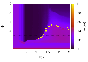
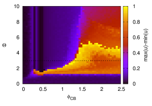
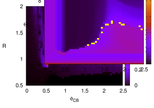
Figure 6: A more systematic diagram of the effect observed in Fig. 5. Here we move on the diagonal $\phi_{\pi}=\phi_{\varepsilon}$ of Fig. 5 on the $\phi_{\text{CB}}$-axis and plot the average unemployment $u$ and unemployment variations $\max_{t}(u)-\min_{t}(u)$. The other axis is either $\Theta$ (top row, for $R=2$) or $R$ (bottom row, for $\Theta=10$), still with $\alpha_{\Gamma}=50$, $\alpha_{c}=4.$, $\pi^{*}=0.2\%$ and $u^{*}=0.05$. Note that since $\alpha_{\Gamma}>0$, the transition at $R_{c}\approx 1,\phi_{\text{CB}}=0$ is second order (see Appendix B). As above, yellow/orange regions in the plots on the right, correspond to unstable economies with crises of large amplitude.

As a complement to the above analysis we also investigated the performance of the policy as a function of the distance between target and natural values. We find, not surprisingly, that when targets are not too far from the natural state of the economy the CB manages to achieve its targets without triggering any instability. When however targets are far from the natural state even a mild policy may become detrimental and trigger instabilities.

IV.4 The role of households and firms sensitivity to rates

We have also investigated the role of the two policy transmission channels ($\alpha_{\Gamma}$, firms and $\alpha_{c}$, households) separately, and found that both channels in isolation may trigger instabilities. In Fig. 7 we plot the policy performance in the $(\phi_{\text{CB}},\alpha_{c})$ plane and the $(\phi_{\text{CB}},\alpha_{\Gamma})$ plane, with all other parameters fixed, in particular $R=2$ and $\Theta=3$. As expected, the top row shows that the larger the value of $\alpha_{c}$, the more careful the monetary policy has to be in order to avoid instabilities. Note, interestingly, that there is a thin region in the $(\phi_{\text{CB}},\alpha_{c})$ plane (spot the yellow dots) where unemployment goes to $u\approx 1$, i.e. the economy is completely destabilized by the monetary policy!

The bottom row of Fig. 7 shows the interplay between policy aggressiveness $\phi_{\text{CB}}$ and firms sensitivity to the real interest rate $\alpha_{\Gamma}$. When $\phi_{\text{CB}}=0$, one recovers the FE-RU transition for $\alpha_{\Gamma}\approx 30$ already observed in Fig. 2. For larger $\alpha_{\Gamma}$’s, the CB policy is at first successful in reinstalling the FE phase, before destabilizing again the economy beyond $\phi_{\text{CB}}^{*}\approx 0.9$. When $\alpha_{\Gamma}$ becomes small, a portion of the FE region expands up to higher values of $\phi_{\text{CB}}\approx 1.25$.

A detailed comparison between Fig. 6 (top row) and Fig. 7 (bottom row) reveals that the simultaneous presence of the two transmission channels has an overall stabilizing effect. Indeed, when only one channel is present (i.e. either $\alpha_{c}$ or $\alpha_{\Gamma}$ is zero) the value of $\phi_{\text{CB}}$ beyond which the system is unstable is smaller than when both channels are active. For example, for $\Theta=3$, $\alpha_{c}=4.$ and $\alpha_{\Gamma}=50.$ one sees from Fig. 6 (top row; left, horizontal line) that the economy is destabilized for $\phi_{\text{CB}}^{*}\approx 1.3$, to be compared to $\phi_{\text{CB}}^{*}\approx 0.9$ when $\alpha_{c}=0$ and to $\phi_{\text{CB}}^{*}\approx 0.5$ when $\alpha_{\Gamma}=0$. Although we cannot provide a complete interpretation, this interesting observation might be due to the fact that the $\alpha$ parameters can be interpreted as “awareness” parameters that allow firms and agents to better anticipate crises and thus dampen the destabilising influence of the Central Bank policy.

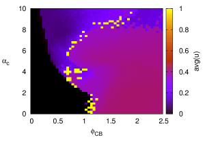
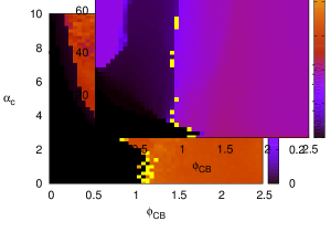
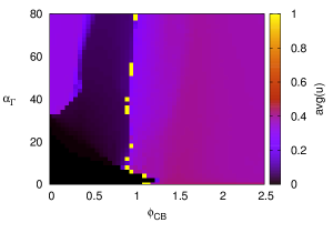
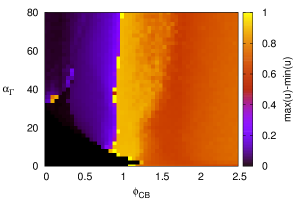
Figure 7: Policy performance, as in the previous two plots, now separately as a function of the households sensitivity to rates $\alpha_{c}$ and the firms sensitivity to rates $\alpha_{\Gamma}$. The $x$-axis is again $\phi_{\pi}=\phi_{\varepsilon}\equiv\phi_{\text{CB}}$, whereas $\Theta=3$, $R=2$ and $\rho^{*}=2\%$, with again $\pi^{*}=0.2\%$ and $u^{*}=0.05$. (Top row) Here $\alpha_{\Gamma}=0$ and $\alpha_{c}>0$. The FE (black) region prevailing for $\alpha_{c}=\phi_{\text{CB}}=0$ is destabilized beyond a certain $\phi_{\text{CB}}^{*}$ that decreases as $\alpha_{c}$ increases. Note the constellation of yellow points that correspond to a completely broken economy. (Bottom row) We now set $\alpha_{c}=0$ and vary $\alpha_{\Gamma}>0$. When $\phi_{\text{CB}}=0$, one recovers the FE-RU transition for $\alpha_{\Gamma}\approx 30$ observed in Fig. 2. One sees that for larger $\alpha_{\Gamma}$’s, the CB policy is at first successful in reinstalling the FE phase, before destabilizing again the economy beyond the vertical line $\phi_{\text{CB}}^{*}\approx 0.9$.

IV.5 Comparison with DSGE models

It is quite interesting to compare the diagram of Fig. 5 with its DSGE counterpart (see e.g DSGE , section 4.3). Within our Agent-Based framework, small values of $\phi_{\pi},\phi_{\varepsilon}$ are at worst ineffective wheras large values of $\phi_{\pi},\phi_{\varepsilon}$ lead to instabilities. This is at the opposite of what is observed in the fully rational world of DSGE models, where small values of $\phi_{\pi},\phi_{\varepsilon}$ lead to instabilities, while large values of $\phi_{\pi},\phi_{\varepsilon}$ allow the Central Bank to funnel the economy on a stability path DSGE . The intuition for this is made crystal clear by Galì in DSGE : The monetary authority should respond to deviations of inflation and the output gap from their target levels by adjusting the nominal rate with “sufficient strength”; […] it is the presence of a “threat” of a strong response by the monetary authority to an eventual deviation of the output gap and inflation from target that suffices to rule out any such deviation in equilibrium. In other words, fully rational, forward looking agents know that inflation will be tamed by the response of central authorities, an element that is indeed completely absent in the myopic forecast world of most ABMs (including Mark-0), where agents only use their knowledge of the past and present situation and adapt their behavior accordingly. The fact that the outcome of these two hypotheses on the stability of the economy are so radically different should be a strong caveat. Which of these two extreme visions of the world is closest to reality is of course a matter of empirical investigation (on this point, see Hommes-DSGE , and for recent attempts to include deviations from perfect rationality in DSGE models, see e.g. Woodford ).

V Summary, Conclusion

In this paper, we parsimoniously extended the stylized macroeconomic Agent-Based Mark-0 model introduced in Tipping , with the aim of investigating the role and efficacy of monetary policy. We focused on three effects induced by a non-zero interest rate in the model, that are arguably the most important transmission channels of the Central Bank policy: i) a change of the accounting rules to factor in the cost of debt and the extra revenue of deposits; ii) a change of the consumption behavior of household that depends negatively on the real interest rate and iii) a change in the hiring/firing and wage policies of firms, that avoid running into debt when interest rates increase. This amounts to adding only two new parameters to the baseline Mark-0 model of Tipping .

We first studied the model in the absence of monetary policy, i.e. without a “Taylor-rule” that creates a feedback between inflation, unemployment and interest rates. The introduction of a coupling between the financial fragility of firms and the hiring/firing and wage policies has two main effects: a) the first order (discontinuous) phase transition between a ‘good’ and a ‘bad’ phase of the economy, discussed in Tipping is replaced by a second order (continuous) transition; b) a new first order transition to a phase with high residual unemployment (RU) appears when the interest rate is larger than some critical value, even in the region where full employment (FE) is achieved for zero-interest rate (i.e. $\Theta\gg 1$ in Fig. 1). The larger the sensitivity to interest rates, the smaller the value of the baseline rate beyond which the economy is destabilized. In that region, allowing firms to accumulate more debt does not help stabilizing the economy.

We then allowed the Central Bank to adjust the baseline rate so as to steer the economy towards prescribed levels of inflation and employment. Our major finding is that provided its policy is not too aggressive (i.e. when the targets are not too far from the ‘natural’ state of the economy, and for a low enough adjustment speed) the Central Bank is successful in achieving its goals. However, the mere presence of different states of the economy separated by phase boundaries, besides being interesting per se, can cause the monetary policy itself to trigger instabilities and be counter-productive. The destabilizing influence of the Central Bank also depends on the firms/households sensitivities to rates. Perhaps ironically, too small sensitivities make the Central Bank policy inefficient, but too large sensitivities make the same policy dangerous. Seen differently, the Central Bank must navigate in a narrow window: too little is not enough, too much leads to instabilities and wildly oscillating economies Felix . As mentioned in the last paragraph, this conclusion strongly contrasts with the prediction of DSGE models. Interestingly, we also find that a Central Bank with a dual mandate (inflation and output) enjoys a wider region of stability compared to a Central bank with inflation as the only mandate.

As we emphasized in the introduction, the key message of both our previous paper Tipping and the present one is that even over-simplified macroeconomic ABMs generically display a rich phenomenology with an economy characterized by different states separated by phase boundaries across which radical changes of the emergent behavior take place. These are, we believe, the “dark corners” alluded to by O. Blanchard in Blanchard , that both academics and policy makers should account for and wrestle with. We believe that the major advantage of ABMs over DSGE-like models is the very possibility of crises at the aggregate level, mediated by generic feedback mechanisms whose destabilizing role may not be immediately obvious or intuitive. Rather than the precisely calibrated predictive tools that standard equilibrium models claim to provide Caballero , ABMs offer extremely valuable qualitative tools for generating scenarios, that can be used to foresee the unintended consequences of some policy decisions. Some of this outcomes, which would be “Black Swans” Taleb in a DSGE framework, can in fact be fully anticipated by schematic ABMs Foley . As expressed with remarkable insight by Mark Buchanan Buchanan : Done properly, computer simulation represents a kind of “telescope for the mind,” multiplying human powers of analysis and insight just as a telescope does our powers of vision. With simulations, we can discover relationships that the unaided human mind, or even the human mind aided with the best mathematical analysis, would never grasp.

Appendix A Price, production and wage updates

A.1 The households timeline

• At the beginning of the time step households are characterized by a certain amount of savings $S(t)\geq 0$.

• After each firm chooses its production $Y_{i}(t)$, price $P_{i}(t)$ and wage $W_{i}(t)$ for the current time step (see later) wages are paid. Since firms use a one-to-one linear technology taking only labor as input and productivity is set to $1$, the production equal the workforce of the firm. Hence, the total amount of wages paid is given by

  $$W_{T}(t)=\sum_{i}W_{i}(t)Y_{i}(t)$$ (14)

• Once the total payroll of the economy is determined, interests on deposits are paid and households set a consumption budget as

  $$C_{B}(t)=c(t)[S(t)+W_{T}(t)+\rho^{\text{d}}(t)S(t)]$$ (15)

  where $c(t)\in[0,1]$ is the propensity to consume and may depend on inflation/interests on deposits, see Eq. (9).

• The consumption budget is distributed among firms using an intensity of choice model Anderson . The demand of goods for firm $i$ is therefore:

  $$D_{i}(t)=\frac{C_{B}(t)}{p_{i}(t)}\frac{e^{-\beta p_{i}(t)/\overline{p}(t)}}{\sum_{i}e^{-\beta p_{i}(t)/\overline{p}(t)}}\ ,$$ (16)

  where $\beta$ is the price sensitivity parameter determining an exponential dependence of households demand to the price offered by the firm. Indeed, $\beta=0$ corresponds to complete price insensitivity and $\beta\rightarrow\infty$ means that households select only the firm with the lowest price. In this sense, as long as $\beta>0$ firms compete on prices.

• The actual consumption $C(t)$ (limited by production) is given by

  $$C(t):=\sum_{i=1}^{N_{\rm F}}p_{i}(t)\min{\{Y_{i}(t),D_{i}(t)\}}\leq C_{B}(t)=\sum_{i=1}^{N_{\rm F}}p_{i}(t)D_{i}(t)$$ (17)

  and households accounting therefore reads

  $$S(t+1)=[1+\rho^{\text{d}}(t)]S(t)+W_{T}(t)-\sum_{i}P_{i}(t)\min{\{D_{i},Y_{i}\}}+\Delta(t)$$ (18)

  where $\Delta(t)$ are dividends paid (see below for a definition of this last term).

A.2 The firms timeline

• At the beginning of the time step $t$ firms with $\Phi_{i}(t)\geq\Theta$ become inactive and are removed from the simulation. Default costs are computed as

  $${\cal D}(t)=-\sum_{i\ \mbox{\footnotesize bankrupt}}{\cal E}_{i}(t)\ .$$ (19)

  Firms with $\Phi_{i}(t)<\Theta$ are instead allowed to continue their activity and contribute to total loans ${\cal E}^{-}(t)$ and total firms savings ${\cal E}^{+}(t)$ as

  $${\cal E}^{-} = -\sum_{i\ \mbox{\footnotesize not bankrupt}}\min{\{{\cal E}_{i}(t),0\}}$$

  $${\cal E}^{+} = \sum_{i\ \mbox{\footnotesize not bankrupt}}\max{\{{\cal E}_{i}(t),0\}}.$$ (20)

• Active firms set production, price and wage for the current time step following simple adaptive rules which are meant to represent an heuristic adjustment. In particular:

  1. Price:
     Prices are updated through a random multiplicative process which takes into account the production-demand gap experienced in the previous time step and if the price offered is competitive (with respect to the average price). The update rule for prices reads:

     $$\begin{split}\text{If }Y_{i}(t)<D_{i}(t)&\hskip 10.0pt\Rightarrow\hskip 10.0pt\begin{cases}&\text{If }p_{i}(t)<\overline{p}(t)\hskip 10.0pt\Rightarrow\hskip 10.0ptp_{i}(t+1)=p_{i}(t)(1+\gamma_{p}\xi_{i}(t))\\ &\text{If }p_{i}(t)\geq\overline{p}(t)\hskip 10.0pt\Rightarrow\hskip 10.0ptp_{i}(t+1)=p_{i}(t)\\ \end{cases}\\ \text{If }Y_{i}(t)>D_{i}(t)&\hskip 10.0pt\Rightarrow\hskip 10.0pt\begin{cases}&\text{If }p_{i}(t)>\overline{p}(t)\hskip 10.0pt\Rightarrow\hskip 10.0ptp_{i}(t+1)=p_{i}(t)(1-\gamma_{p}\xi_{i}(t))\\ &\text{If }p_{i}(t)\leq\overline{p}(t)\hskip 10.0pt\Rightarrow\hskip 10.0ptp_{i}(t+1)=p_{i}(t)\\ \end{cases}\end{split}$$ (21)

     where $\xi_{i}(t)$ are independent uniform $U[0,1]$ random variables and $\gamma_{p}$ is a parameter setting the relative magnitude of the price adjustment (we set it to $5\%$ unless stated otherwise). Fig. 8, which plots the average profit of firms as a function of the offered price, shows that these rules lead to a reasonable emergent “optimizing” behavior of firms. As expected, the profit reaches a maximum for prices slightly above the average price $\overline{p}(t)$. Higher prices are not competitive and firms lose clients, while lower prices do not cover production costs.

     

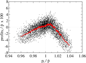
     Figure 8: Scatter plot in one time step of firm profits vs the price offered. The red line correspond to a moving flat average of $100$ consecutive points. Parameters are: $R=2$ (with $\eta^{0}_{-}=0.1$), $\Theta=2$, $\gamma_{p}=\gamma_{w}=0.05$, $\alpha_{\Gamma}=50$, $\Gamma_{0}=0$, $\beta=2$, $\alpha_{c}=4$, $N=5000$ and $\rho^{*}=0.5\%$.

  2. Production:
     Independently of their price level, firms try to adjust their production to the observed demand. When firms want to hire, they open positions on the job market; we assume that the total number of unemployed workers, which is $N_{\rm F}u(t)$, is distributed among firms according to an intensity of choice model which depends on both the wage offered by the firm and on the same parameter $\beta$ as it is for Eq. (16); therefore the maximum number of available workers to each firm is:

     $$u^{*}_{i}(t)=\frac{e^{\beta W_{i}(t)/\overline{w}(t)}}{\sum_{i}e^{\beta W_{i}(t)/\overline{w}(t)}}N_{\rm F}u(t)\ .$$ (22)

     The production update is then defined as:

     $$\begin{split}\text{If }Y_{i}(t)<D_{i}(t)&\hskip 10.0pt\Rightarrow\hskip 10.0ptY_{i}(t+1)=Y_{i}(t)+\min\{\eta^{+}_{i}(D_{i}(t)-Y_{i}(t)),u^{*}_{i}(t)\}\\ \text{If }Y_{i}(t)>D_{i}(t)&\hskip 10.0pt\Rightarrow\hskip 10.0ptY_{i}(t+1)=Y_{i}(t)-\eta^{-}_{i}[Y_{i}(t)-D_{i}(t)]\\ \end{split}$$ (23)

     where $\eta^{\pm}\in[0,1]$ are what we denote as the hiring/firing propensity of the firms. According to this mechanism, the change in output responds to excess demand (there is an increase in output if excess demand is positive, a decrease in output if excess demand is negative, i.e. if there is excess supply). The propensities to hire/fire $\eta_{\pm}$ are the sensitivity of the output change to excess demand/supply.

  3. Wage:
     The wage update rule we chose follows (in spirit) the choices made for price and production. We propose that at each time step firm $i$ updates its wage as:

     $$\begin{split}W^{T}_{i}(t+1)=W_{i}(t)[1+\gamma_{w}(1-\Gamma\Phi_{i})\varepsilon\xi^{\prime}_{i}(t)]\quad\mbox{if}\quad\begin{cases}Y_{i}(t)&<D_{i}(t)\\ {\cal P}_{i}(t)&>0\end{cases}\\ W_{i}(t+1)=W_{i}(t)[1-\gamma_{w}(1+\Gamma\Phi_{i})u\xi^{\prime}_{i}(t)]\quad\mbox{if}\quad\begin{cases}Y_{i}(t)&>D_{i}(t)\\ {\cal P}_{i}(t)&<0\end{cases}\end{split}$$ (24)

     where $\gamma_{w}$ is a certain parameter, ${\cal P}_{i}(t)$ is the profit of the firm at time $t$ and $\xi^{\prime}_{i}(t)$ an independent $U[0,1]$ random variable. If $W^{T}_{i}(t+1)$ is such that the profit of firm $i$ at time $t$ with this amount of wages would have been negative, $W_{i}(t+1)$ is chosen to be exactly at the equilibrium point where ${\cal P}_{i}(t)=0$ otherwise $W_{i}(t+1)=W^{T}_{i}(t+1)$.

     The above rules are intuitive: if a firm makes a profit and it has a large demand for its good, it will increase the pay of its workers. The pay rise is expected to be large if the firm is financially healthy and/or if unemployment is low (i.e. if $\varepsilon$ is large) because pressure on salaries is high. Conversely, if the firm makes a loss and has a low demand for its good, it will reduce the wages. This reduction is drastic if the company is close to bankruptcy, and/or if unemployment is high, because the pressure on salaries is then low. In all other cases, wages are not updated.

     The parameters $\gamma_{p,w}$ allow us to simulate different price/wage update timescales, i.e. the aggressivity with which firms react a change of their economic conditions. In the following we set $\gamma_{p}=0.05$ and $\gamma_{w}=\gamma_{p}$. The case $\gamma_{w}=0$ corresponds to removing completely the wage update rule, such that the version of the model with constant wage is recovered.

• After prices, productions and wages are set and interests paid, consumption and accounting take place. Since each firm has total sales $p_{i}\min{\{Y_{i},D_{i}\}}$ firms profits are

  $${\cal P}_{i}(t)=p_{i}(t)\min{\{Y_{i}(t),D_{i}(t)\}}-W_{i}(t)Y_{i}(t)+\rho^{\text{d}}\max{\{{\cal E}_{i}(t),0\}}+\rho^{\ell}\min{\{{\cal E}_{i}(t),0\}}\ .$$ (25)

  When firms have both positive ${\cal E}_{i}$ and ${\cal P}_{i}$ dividends are paid as a fraction $\delta$ of the firm cash balance ${\cal E}_{i}$. The update rule for firms cash balance is therefore

  $${\cal E}_{i}(t+1)={\cal E}_{i}(t)+{\cal P}_{i}(t)-\delta{\cal E}_{i}(t)\theta({\cal P}_{i}(t))\theta({\cal E}_{i}(t))$$ (26)

  where $\theta(x)=1$ if $x>0$ and $0$ otherwise. Correspondingly, households savings are updated as

  $$S(t+1)=S(t)+\sum_{i}W_{i}(t)Y_{i}(t)-\sum_{i}p_{i}(t)\min{\{Y_{i}(t),D_{i}(t)\}}+\delta\sum_{i}{\cal E}_{i}(t)\theta({\cal P}_{i}(t))\theta({\cal E}_{i}(t)).$$ (27)

  The dividends share $\delta$ is set to $2\%$ unless stated otherwise and the $\Delta(t)$ term in Eq. (18) is given by

  $$\Delta(t)=\delta\sum_{i}{\cal E}_{i}(t)\theta({\cal P}_{i}(t))\theta({\cal E}_{i}(t))$$ (28)

• Finally, an inactive firm has a finite probability $\varphi$ (which we set to $0.1$) per unit time to get revived; when it does so its price is fixed to $p_{i}(t)=\overline{p}(t)$, its wage to $w_{i}(t)=\overline{w}(t)$, its workforce is the available workforce $Y_{i}(t)=\mu u(t)$ and its cash-balance is the amount needed to pay the wage bill ${\cal E}_{i}(t)=W_{i}(t)Y_{i}(t)$. This small ’liquidity’ is provided by firms with positive ${\cal E}_{i}$ in shares proportional to their wealth ${\cal E}_{i}$.

Appendix B Firms’ adaptive behavior leads to a second order phase transition

We start by analysing the effect of adaptation of firms. In order to get a first insight it is useful to consider a simplified setting where $\Gamma=\Gamma_{0}$ (i.e. $\alpha_{\Gamma}=0$), $\rho^{\ell}(t)=\rho_{0}(t)=0$, $f=1$, $c(t)=c_{0}=0.5$ (hence $\alpha_{c}=0$) and wages are constant and equal to $1$ ($\gamma_{w}=0$). In this case the basic model described in Tipping (with constant wages) is recovered.

Intuitively, the coupling between financial fragility and hiring/firing propensity should have a stabilizing effect on the economy. Moreover, the full unemployment phase at $R<R_{c}$ is deeply affected by the presence of $\alpha_{\Gamma}$: for $\alpha_{\Gamma}\neq 0$ the unemployment rate in this phase is no longer one, but becomes smaller than one and continuously changing with $R$. In order to derive an estimate of these continuous values we use an intuitive argument (at $\Theta=\infty$) which is justified a posteriori by the good match with numerical results. Given the critical ratio $R=\eta^{0}_{+}/\eta^{0}_{-}=R_{c}$ separating the high/low unemployment phases when there is no adaptation (i.e. $\Gamma_{0}=0$) one can expect that equilibrium values of the unemployment rate different from $0$ and $1$ can only be stable if $\eta_{+}^{i}/\eta_{-}^{i}$ remains around the critical value $R_{c}$ at $\Gamma_{0}=0$. Near criticality therefore we enforce that:

$$\frac{\eta_{+}^{i}}{\eta_{-}^{i}}=\frac{\eta^{0}_{+}(1-\Gamma_{0}\Phi_{i})}{\eta^{0}_{-}(1+\Gamma_{0}\Phi_{i})}=R_{c}\hskip 10.0pt\Rightarrow\hskip 10.0pt-\Gamma_{0}\Phi\approx\frac{R_{c}\eta_{-}^{0}-\eta_{+}^{0}}{R_{c}\eta_{-}^{0}+\eta_{+}^{0}}.$$ (29)

An explicit form of $\Phi$ in terms of the employment rate $\varepsilon={\overline{Y}}$ can be obtained with the additional assumption that the system is always close to equilibrium (i.e. $p\approx 1$ and $D\approx Y$, at least when $\eta^{i}_{+}/\eta^{i}_{-}\sim R_{c}$), which allows one to express households savings in terms of the firms’ production. Indeed (see the discussion in Tipping ) at equilibrium $W=B=N_{\rm F}Y=c(W+S)$, from which it follows that $N_{\rm F}Y=W=Sc/(1-c)$. For $c=0.5$ as in our simulations one thus has $S=N_{\rm F}Y$. Since the total amount of money is conserved (in our simulations $N_{\rm F}\overline{{\cal E}}+S=N_{\rm F}\overline{{\cal E}}+N_{\rm F}Y=N_{\rm F}$, see Appendix C) one finally obtains that $\overline{{\cal L}}=1-Y$ and $\Phi=(Y-1)/Y=(\varepsilon-1)/\varepsilon$, hence

$$\frac{\Gamma_{0}}{\varepsilon}=\frac{R_{c}\eta_{-}^{0}-\eta_{+}^{0}}{R_{c}\eta_{-}^{0}+\eta_{+}^{0}}+\Gamma_{0}=\frac{R_{c}-R}{R_{c}+R}+\Gamma_{0}\ .$$ (30)

Note that according to this formula the employment goes to $\varepsilon=1$ at the critical point $R=R_{c}$. Above this value, the economy is in the “good” state and employment sticks to $\varepsilon=1$ (this is because in the argument the effect of $\Theta$ has been neglected). Moreover, when $R=R_{c}$, $\varepsilon$ is proportional to $\Gamma_{0}$ and therefore in the limit $\Gamma_{0}\rightarrow 0$ one has $\varepsilon=0$ for all $R<R_{c}$. This is the “bad” phase of full unemployment at $\Gamma_{0}=0$, which becomes in this case a phase where employment grows steadily but remains of order $\Gamma_{0}$ except very close to the critical point.

Eq. (30) is plotted in Fig. 9 together with numerical results. Note that in this case the representative firm approximation ($N_{\rm F}=1$) is in good agreement with numerical results also for $N_{\rm F}=10,000$, as it was for the discontinuous transition obtained for $\Gamma=0$. In the inset of Fig. 9 one can see that the variance of the fluctuations of employment rate is diverging as long as the critical value of $R$ is approached. This is confirmed by a spectral analysis of the unemployment time series (see Fig. 10). In order to obtain the power spectrum we apply the GSL Fast Fourier Transform algorithm to the time series $\varepsilon(t)-\langle\varepsilon\rangle$. As one can see in Fig. 10 the power spectrum is well approximated by an Ornstein-Uhlenbeck form:

$$I(\omega)=I_{0}\frac{\omega_{0}^{2}}{\omega_{0}^{2}+\omega^{2}}$$ (31)

with $\omega_{0}$ going linearly to $0$ when $\eta^{0}_{+}$ approaches its critical value, meaning that the relaxation time $\omega_{0}^{-1}$ diverges as one approaches the critical point. Note that this is not the case for the Mark 0 model with $\Gamma_{0}=0$ which instead has a white noise power spectrum even in proximity of the transition line. The first order (discontinuous) transition for $\Gamma_{0}=0,\Theta=\infty$ is thus replaced by a second order (continuous) transition when the firms adapt their behavior as a function of their financial fragility.

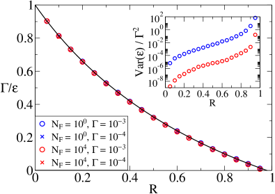
Figure 9: Inverse of the average employment rate $\Gamma_{0}/\overline{\varepsilon}$ as a function of the ratio $R=\eta^{0}_{+}/\eta^{0}_{-}$ with $\eta^{0}_{-}=0.1$ and $\gamma=0.01$ when $\Gamma_{0}>0$. When the employment rate is rescaled with the parameter $\Gamma_{0}$ (here $\Gamma_{0}=10^{-3},\ 10^{-4}$) the different lines collapse and Eq. (30) agrees with numerical simulations. In the inset we also plot the rescaled variance, still as a function of $\eta^{0}_{+}$. Approaching the critical point the variance of the unemployment fluctuations diverges, together with their relaxation time going to infinity. The other parameters are: $\delta=0.02$, $\Theta=5$, $\gamma_{w}=0$, $c=0.5$, $\beta=0$ and $\varphi=0.1$

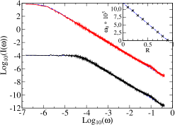
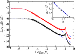
Figure 10: Logarithm of the normalized power spectrum for Mark 0 with adaptive firms ($\Gamma_{0}=10^{-3}$), $\gamma_{p}=0.05$ and $N_{\rm F}=1$ (left) and $N_{\rm F}=1000$ (right). The other parameters are set as in Fig. 9. The main plot shows two examples of the spectrum for $\eta_{-}^{0}=0.1$ and $\eta_{+}^{0}=0.05$ (black line) and $\eta^{0}_{+}=0.09$ (red line) in the left plot, $\eta_{+}^{0}=0.05$ (black line) and $\eta^{0}_{+}=0.08$ (red line) in the right plot. The time series is made of $2^{28}$ time steps after $T_{eq}=500\,000$ and the logarithm of the spectrum is averaged over a moving window of $100$ points for a better visualization. With both system sizes the fit with Eq. (31) (blue dashed lines) is good with the only difference that when $N_{\rm F}>1$ a clear oscillatory pattern appears at high frequencies, that becomes sharper and sharper as $N_{\rm F}$ increases. In the inset of each figure we plot the value of $\omega_{0}$ in Eq. (31) obtained from the fit as a function of the ratio $R=\eta_{+}^{0}/\eta_{-}^{0}$. In both cases $\omega_{0}$ goes linearly to $0$ as the critical value is approached.

Finally, note that the presence of a continuum of states for the unemployment rate whenever $\Gamma_{0}>0$ and $R<R_{c}$ holds also with $\gamma_{w}>0$ (when wages are not constant). It was however simpler to perform analytical computations with constant wages.

Appendix C Pseudo-code of Mark 0

We present here the pseudo-code for the Mark 0 code described in Sec. II.2 and Appendix A. The source code of the baseline Mark-0 is available on demand.

Algorithm 1 Mark 0

$N_{\rm F}$ Number of firms; $c_{0},\beta,\gamma_{p},\gamma_{w},\eta^{0}_{+},\eta^{0}_{-},\delta,\Theta,\varphi,f,\alpha_{c},\phi_{\pi},\phi_{\varepsilon},\alpha_{\Gamma},\Gamma_{0},\varepsilon^{*},\pi^{*},\rho^{*},\omega$; $T$ total evolution time;

$\triangleright$ Initialization

for ($i\leftarrow 0;i<N_{\rm F};i\leftarrow i+1$) do

     $W[i]\leftarrow 1$

     $p[i]\leftarrow 1+0.2(\text{\tt random}-0.5)$

     $Y[i]\leftarrow[1+0.2(\text{\tt random}-0.5)]/2$

     $D[i]\leftarrow 0.5$ $\triangleright$ Initial employment is $0.5$

     ${\cal E}[i]\leftarrow W[i]Y[i]\,\text{\tt random}$

     ${\cal P}[i]\leftarrow p[i]\min(D[i],Y[i])-W[i]Y[i]$

     $a[i]\leftarrow 1$ $\triangleright$ binary variable: active ($1$) / inactive ($0$) firm

end for

$S\leftarrow N_{\rm F}-\sum_{i}{\cal E}[i]$ $\triangleright$ Main loop

for ($t\leftarrow 1;t\leq T;t\leftarrow t+1$) do

     $\varepsilon\leftarrow\frac{1}{N_{\rm F}}\sum_{i}Y[i]$

     $u\leftarrow 1-\varepsilon$

     $\overline{p}\leftarrow\frac{\sum_{i}p[i]Y[i]}{\sum_{i}Y[i]}$

     $\overline{w}\leftarrow\frac{\sum_{i}W[i]Y[i]}{\sum_{i}Y[i]}$

     $u^{*}[i]\leftarrow\frac{\exp(\beta W[i]/\overline{w})}{\sum_{i}a[i]\exp(\beta W[i]/\overline{w})}N_{\rm F}u$

     $\widetilde{x}\leftarrow\omega x+(1-\omega)\widetilde{x}$ where $x$ are $\pi,\rho^{\text{d}},\rho^{\ell},u$ $\triangleright$ Central Bank policy

     $\hat{\varepsilon}^{*}\leftarrow\min{(\varepsilon^{*},1.025\tilde{\varepsilon})}$

     $\rho_{0}\leftarrow\rho^{*}+10\phi_{\pi}(\tilde{\pi}-\pi^{*})+\phi_{\varepsilon}\log{(\tilde{\varepsilon}/\hat{\varepsilon}^{*})}$

     $\rho_{0}\leftarrow\max{(\rho_{0},0)}$

     $\Gamma\leftarrow\max{\{\alpha_{\Gamma}(\widetilde{\rho}^{\ell}-\widetilde{\pi}),\Gamma_{0}\}}$

     $\mathcal{D}\leftarrow{\cal E}^{-}\leftarrow{\cal E}^{+}\leftarrow 0$ $\triangleright$ Firms update prices, productions and wages

     for ($i\leftarrow 0;i<N_{\rm F};i\leftarrow i+1$) do

         if  $a[i]==1$  then

              if ${\cal E}[i]>-\Theta W[i]Y[i]$ then

                  ${\cal E}^{+}\leftarrow{\cal E}^{+}+\max{\{{\cal E}[i],0\}}$

                  ${\cal E}^{-}\leftarrow{\cal E}^{-}-\min{\{{\cal E}[i],0\}}$

                  $\Phi[i]\leftarrow-\frac{{\cal E}[i]}{W[i]Y[i]}$

                  $\Phi[i]\leftarrow\min{\{\Phi[i],1/\Gamma\}}$

                  $\Phi[i]\leftarrow\max{\{\Phi[i],-1/\Gamma\}}$

                  $\eta_{+}\leftarrow\eta^{0}_{+}(1-\Gamma\Phi[i])$

                  $\eta_{-}\leftarrow\eta^{0}_{-}(1+\Gamma\Phi[i])$

                  

                  if  $Y[i]<D[i]$  then

                       if ${\cal P}[i]>0$ then

                           $W[i]\leftarrow W[i][1+\gamma_{w}(1-\Gamma\Phi[i])\varepsilon$ random$]$

                           $W[i]\leftarrow\min{\{W[i],(P[i]\min{[D[i],Y[i]]}+\rho^{\text{d}}\max{\{{\cal E}[i],0\}}+\rho^{\ell}\min{\{{\cal E}[i],0\}})/Y[i]\}}$

                       end if

                       $Y[i]\leftarrow Y[i]+\min\{\eta_{+}(D[i]-Y[i]),u^{*}[i]\}$

                       if  $p[i]<\overline{p}$ then $p[i]\leftarrow p[i](1+\gamma_{p}\,$random)

                       end if

                  else if  $Y[i]>D[i]$  then

                       if ${\cal P}[i]<0$ then

                           $W[i]\leftarrow W[i][1-\gamma_{w}(1+\Gamma\Phi[i])u$ random$]$

                       end if

                       $Y[i]\leftarrow\max\{0,Y[i]-\eta_{-}(D[i]-Y[i])\}$

                       if  $p[i]<\overline{p}$  then $p[i]\leftarrow p[i](1-\gamma_{p}\,$random)

                       end if

                  end if

              else if ${\cal E}[i]\leq-\Theta W[i]Y[i]$ then

                  $a[i]\leftarrow 0$

                  $\mathcal{D}\leftarrow\mathcal{D}-{\cal E}[i]$

              end if

         end if

     end for

Algorithm 2 Mark0 (continued)

     

     $u\leftarrow 1-\frac{1}{N_{\rm F}}\sum_{i}Y[i]$ $\triangleright$ Update $u$ and $\overline{p}$

     $\overline{p}\leftarrow\frac{\sum_{i}p[i]Y[i]}{\sum_{i}Y[i]}$

     $\triangleright$ Private bank sets interest rates

     $\rho^{\ell}=\rho_{0}+(1-f)\mathcal{D}/{\cal E}^{-}$

     $\rho^{\text{d}}=\frac{\rho^{\ell}{\cal E}^{-}-\mathcal{D}}{S+{\cal E}^{+}}$

     $\triangleright$ Households decide the demand

     $S\leftarrow(1+\rho^{\text{d}})S+\sum_{i}W[i]Y[i]$

     $c\leftarrow c_{0}[1+\alpha_{c}(\widetilde{\pi}-\widetilde{\rho}^{\text{d}})/\gamma_{\pi}]$

     $C_{B}\leftarrow cS$

     

     for ($i\leftarrow 0;i<N_{\rm F};i\leftarrow i+1$) do

         $D[i]\leftarrow\frac{C_{B}a[i]\exp(-\beta p[i]/\overline{p})}{p[i]\sum_{i}a[i]\exp(-\beta p[i]/\overline{p})}$ $\triangleright$ Inactive firms have no demand

     end for

     $\triangleright$ Accounting

     ${\cal E}^{+}\leftarrow 0$

     for ($i\leftarrow 0;i<N_{\rm F};i\leftarrow i+1$) do

         if  $a[i]==1$  then

              $S\leftarrow S-p[i]\min\{Y[i],D[i]\}$

              ${\cal P}[i]\leftarrow p[i]\min\{Y[i],D[i]\}-W[i]Y[i]+\rho^{\text{d}}\max{\{{\cal E}[i],0\}}+\rho^{\ell}\min{\{{\cal E}[i],0\}}$

              ${\cal E}[i]\leftarrow{\cal E}[i]+{\cal P}[i]$

              if  ${\cal P}[i]>0$ && ${\cal E}[i]>0$  then $\triangleright$ Pay dividends

                  $S\leftarrow S+\delta\,{\cal E}[i]$

                  ${\cal E}[i]\leftarrow{\cal E}[i]-\delta\,{\cal E}[i]$

              end if

              ${\cal E}^{+}\leftarrow{\cal E}^{+}+\max{\{{\cal E}[i],0\}}$

         end if

     end for

     $\triangleright$ Revivals

     $\mathcal{R}\leftarrow 0$

     for ($i\leftarrow 0;i<N_{\rm F};i\leftarrow i+1$) do

         if  $a[i]==0$ then

              if  random $<\varphi$  then

                  $Y[i]\leftarrow u\mbox{ random}$

                  $a[i]\leftarrow 1$

                  $P[i]\leftarrow\overline{p}$

                  $W[i]\leftarrow\overline{w}$

                  ${\cal E}[i]\leftarrow W[i]Y[i]$

                  $\mathcal{R}\leftarrow\mathcal{R}+{\cal E}[i]$

                  ${\cal E}^{+}\leftarrow{\cal E}^{+}+\max{\{{\cal E}[i],0\}}$

              end if

         end if

     end for

     for ($i\leftarrow 0;i<N_{\rm F};i\leftarrow i+1$) do

         if $a[i]==1$ then

              if ${\cal E}[i]>0$ then

                  ${\cal E}[i]\leftarrow{\cal E}[i]-\mathcal{R}{\cal E}[i]/{\cal E}^{+}$

              end if

         end if

     end for

end for

References

- (1) S. Gualdi, M. Tarzia, F. Zamponi, J.-P. Bouchaud, Tipping points in macroeconomic agent-based models, Journal of Economic Dynamics and Control 50, 29-61 (2015).
- (2) The Mark I family of models was elaborated in a series of papers and books, in particular: E. Gaffeo, D. Delli Gatti, S. Desiderio, and M. Gallegati, Adaptive Microfoundations for Emergent Macroeconomics, Eastern Economic Journal, 34: 441-463 (2008); D. Delli Gatti, E. Gaffeo, M. Gallegati, G. Giulioni, and A. Palestrini, Emergent Macroeconomics: An Agent-Based Approach to Business Fluctuations, Springer: Berlin, 2008; D. Delli Gatti, S. Desiderio, E. Gaffeo, P. Cirillo, M. Gallegati, Macroeconomics from the Bottom-up, Springer: Berlin (2011).
- (3) see e.g. J. Galí, Monetary Policy, Inflation and the Business Cycle, Princeton University Press (2008).
- (4) for a comparative review of DSGE and macroeconomic ABMs, see: G. Fagiolo, A. Roventini, Macroeconomic Policy in DSGE and Agent-Based Models, Working Paper (2012).
- (5) O. Blanchard, Where Danger Lurks, Finance & Development, September 2014, Vol. 51, No. 3.
- (6) C. Deissenberg, S. van der Hoog, H. Dawid, Eurace: A massively parallel agent-based model of the european economy, Applied Mathematics and Computation, 204: 541-552 (2008); H. Dawid, S. Gemkow, P. Harting, S. van der Hoog, M. Neugarty; The Eurace@Unibi Model: An Agent-Based Macroeconomic Model for Economic Policy Analysis, Working paper, Bielefeld University. 2011.
- (7) G. Dosi, G. Fagiolo, A. Roventini, An evolutionary model of endogenous business cycles. Computational Economics, 27: 3-24 (2005); G. Dosi, G. Fagiolo, and A. Roventini, Schumpeter meeting Keynes: A policyfriendly model of endogenous growth and business cycles, Journal of Economic Dynamics and Control, 34, 1748-1767 (2010); and Review .
- (8) A. Mandel, S. Furst, W. Lass, F. Meissner, C. Jaeger; Lagom generiC: an agent-based model of growing economies, ECF Working Paper 1 /2009.
- (9) S. van der Hoog, H. Dawid, Bubbles, Crashes and the Financial Cycle: Insights from a Stock-Flow Consistent Agent-Based Macroeconomic Model, University of Bielefeld working paper (2015), http://ssrn.com/abstract=2616662.
- (10) S. M. Lein, When do Firms Adjust Prices? Evidence from Micro Panel Data, Journal of Monetary Economics 57, 696-715 (2010).
- (11) S.P. Kothari, J. Lewellen, J. B. Warner, The behavior of aggregate corporate investment, http://ssrn.com/abstract=2511268.
- (12) D. B. Gross, N. S. Souleles, Do Liquidity Constraints and Interest Rates Matter for Consumer Behavior? Evidence from Credit Card Data, Quarterly Journal of Economics, 107, 149-185 (2002); N. S. Souleles, Expectations, Heterogeneous Forecast Errors, and Consumption: Micro Evidence from the Michigan Consumer Sentiment Surveys, Journal of Money, Credit and Banking, 36, 39-72 (2004).
- (13) S. C. Ludvigson, Consumer Confidence and Consumer Spending, Journal of Economic Perspectives, 18, 29-50 (2004).
- (14) M. De Nardi, E. French, and D. Benson, Consumption and the Great Recession, Mimeo, Federal Reserve Bank of Chicago (2012).
- (15) T. Schelling, it Micromotives and Macrobehaviour, W.W. Norton & Co Ltd (1978).
- (16) A. Kirman, The Economic Crisis is a Crisis for Economic Theory, CESifo Economic Studies, 56: 498-535 (2010).
- (17) see e.g. C. Hommes, Behavioral Rationality and Heterogeneous Expectations in Complex Economic Systems, Cambridge University Press (2013) for a review on behavioral experiments, andHommes-DSGE for experiments related to DSGE modelling.
- (18) G. Ehrhardt, M. Marsili, and F. Vega-Redondo, Phenomenological models of socioeconomic network dynamics, Phys. Rev. E 74, 036106 (2006); K. Anand, P. Gai, M. Marsili, The rise and fall of trust networks, Progress in Artificial Economics. Lect. Notes Econ. Math. Syst. 645: 77 (2010).
- (19) M. Marsili, Complexity and financial stability in a large random economy, Quantitative Finance, 14, 1663-1675 (2014).
- (20) P. Gai, A. Haldane, and S. Kapadia, Complexity, concentration and contagion, Journal of Monetary Economics 58, 453-470 (2011).
- (21) J. Batista, J.-P. Bouchaud, D. Challet, Sudden trust collapse in Networked societies, arXiv:1409.8321.
- (22) for a recent review, see: J.-P. Bouchaud, Crises and Collective Socio-Economic Phenomena: Simple Models and Challenges, J. Stat. Phys. 151: 567-606 (2013), and refs. therein.
- (23) A. Chakraborti, D. Challet, A. Chatterjee, M. Marsili, Y.-C. Zhang, B. K Chakrabarti, Statistical mechanics of competitive resource allocation using agent-based models, Physics Reports, 552, 1-25 (2015).
- (24) R. J. Caballero, Macroeconomics after the Crisis: Time to Deal with the Pretense-of-Knowledge Syndrome, Journal of Economic Perspectives, 24: 85-102 (2010).
- (25) L. Tesfatsion, Agent-based computational modeling and macroeconomics, Post Walrasian Macroeconomics: Beyond the Dynamic Stochastic General Equilibrium Model (2006).
- (26) B. LeBaron and L. Tesfatsion,Modeling macroeconomies as open-ended dynamic systems of interacting agents, The American Economic Review (2008): 246-250.
- (27) H. Dawid, G. Fagiolo, Agent-based models for economic policy design: Introduction to the special issue, Journal of Economic Behavior and Organization 67 (2008).
- (28) G. Dosi et al., Fiscal and monetary policies in complex evolving economies, Journal of Economic Dynamics and Control 52 (2015): 166-189.
- (29) G. Dosi et al., Income distribution, credit and fiscal policies in an agent-based Keynesian model, Journal of Economic Dynamics and Control 37.8 (2013): 1598-1625.
- (30) M. Lengnick and H.-W. Wohltmann, Agent-based financial markets and New Keynesian macroeconomics: A synthesis, Journal of Economic Interaction and Coordination 8.1 (2013): 1-32.
- (31) G. Haber, Monetary and fiscal policy analysis with an agent-based macroeconomic model, Jahrbücher für Nationalökonomie und Statistik (2008): 276-295.
- (32) C. Bianchi et al., Validating and calibrating agent-based models: a case study, Computational Economics 30.3 (2007): 245-264.
- (33) G. Fagiolo et al., Empirical validation of agent-based models: A critical survey, No. 2006/14. LEM Working Paper Series, 2006.
- (34) S. Gualdi, J.-P. Bouchaud, G. Cencetti, M. Tarzia and F. Zamponi, ”Endogenous crisis waves: a stochastic model with synchronized collective behavior”, arXiv:1409.3296v1, Phys. Rev. Lett. 114, 088701 (2015).
- (35) N. G. Mankiw. Principles of macroeconomics, Cengage Learning, 2014, see in particular Ch. 14.
- (36) Lawrence J. Christiano, Martin Eichenbaum, and Charles L. Evans, Nominal Rigidities and the Dynamic Effects of a Shock to Monetary Policy, Journal of Political Economy, 113, 1-45 (2005).
- (37) T. Assenza et al., Individual expectations and aggregate macro behavior, Tinbergen Institute Discussion Paper 13-016/II
- (38) K. Adam, M. Woodford, Robustly Optimal Monetary Policy in a Microfounded New Keynesian Model, working paper, http://ssrn.com/abstract=2013817 (2012).
- (39) in this spirit, see the very interesting paper of F. Patzelt and K. Pawelzik, Criticality of Adaptive Control Dynamics, Phys. Rev. Lett. 107: 238103 (2011).
- (40) N. N. Taleb, The Black Swan (London: Random House, 2007).
- (41) D. Farmer, D. Foley, The economy needs agent-based modelling, Nature 460, 685-686 (2009).
- (42) M. Buchanan, This Economy does not compute, New York Times, October 1, 2008. On this topic, see also Kirman ; Foley ; Tipping ; JPB .
- (43) see e.g. S. P. Anderson, A. De Palma, J. F. Thisse, Discrete Choice Theory of Product Differentiation. MIT Press, New York (1992).