Rare B decays using lattice QCD form factors
Abstract:
In this write-up we review and update our recent lattice QCD calculation of , , and form factors [1]. These unquenched calculations, performed in the low-recoil kinematic regime, provide a significant improvement over the use of extrapolated light cone sum rule results. The fits presented here include further kinematic constraints and estimates of additional correlations between the different form factor shape parameters. We use these form factors along with Standard Model determinations of Wilson coefficients to give Standard Model predictions for several observables [2]. The modest improvements to the form factor fits lead to improved determinations of , the fraction of longitudinally polarized vector mesons, but have little effect on most other observables.
1 Introduction
Measurements of the flavor-changing, neutral current (FCNC) decay are rapidly growing in number. In particular, the semi-leptonic FCNC decays of and mesons to the vector mesons, and respectively, have afforded us the opportunity to compare several associated observables with theoretical predictions [3, 4, 5, 6]. The experimental data presently show a few deviations from the Standard Model, including a smaller-than-predicted differential branching fraction in low-recoil kinematic bins. These could be explained by beyond-the-Standard-Model (BSM) contributions to one or two Wilson coefficients in the effective Hamiltonian [7, 8, 9, 10, 2, 11, 12]. However, none of the analyses claim the Standard Model is an unacceptable description of the data. In fact it is not yet certain that all theoretical uncertainties are under firm control.
The largest theoretical uncertainties in these observables are due to QCD interactions. Lattice QCD (LQCD) calculations of the form factors can reduce a class of these uncertainties, improving upon the determinations from sum rules. We recently completed a necessary first step toward accurate, first-principles calculations of the form factors [1]. Below we briefly summarize the results of computing matrix elements of the full basis of currents. The key improvements made compared to previous lattice studies come through using high statistics, physical-mass bottom quarks, and flavors of sea quarks. In Sec. 3 we provide a minor improvement to the method used to fit the form factor shapes. We close in Sec. 4 by touching upon issues which must be confronted in order to improve the theoretical determinations of these observables.
2 Summary of the matrix element calculation
The effective Hamiltonian governing decay is
| (1) |
For the following operators in , matrix elements factorize into local hadronic matrix elements, which are parametrized by seven form factors:
| (2) |
where and . The bulk of this write-up focuses on the details of the form factor calculation and consequences; however, we will comment on contributions to from nonlocal matrix elements and other open issues at the end.
We used a subset of the MILC Collaboration gauge field configurations which include effects of flavors of , tadpole-improved (asqtad) sea quarks. We chose three ensembles, allowing for modest tests of discretization and quark mass effects. We correctly anticipated that obtaining a good signal over statistical noise would be a challenge. In order to address this issue we used eight light quark sources on each configuration, obtaining over 30000 estimates of each correlation function on each of the three ensembles.
The calculations were done with nonrelativistic quarks, formulated in the rest frame and accurate through . The matching of the effective field theory currents to the physical ones, done to , is the source of the largest controlled systematic uncertainty.
The momentum of the or meson varied from to no greater than ( GeV) in magnitude, primarily due to signal-to-noise degradation. Thus the lattice calculations are done in the low recoil regime, i.e. at large , the lepton-pair invariant mass-squared.
From the imaginary-time correlation functions, we performed bootstrapped fits to extract numerical estimates of the seven linearly independent form factors. The basis we use is , , , , , (see [1] for definitions). Once these are determined on each ensemble, for several values of final state momentum, it remains for us to parametrize the shape and give results corresponding to the physical limit.
3 Updated fits
This section describes a minor update of our published results [1]. We fit each form factor, generically denoted , using the following parametrization
| (3) |
where and . Thus the parameters and quantify the dependence of the form factors on the light and strange quark masses, respectively. The splitting between the mass and the relevant resonance is taken to be a fixed value, but variations of up to had no effect on the resulting physical form factors. We determine from a combined fit to , , and data [1] and include it as a Gaussian prior in the subsequent fits to determine , , and . Physical results are obtained by using our fit results for and with . We tried several fits which allowed for discretization effects, but no statistical signal was seen for the corresponding parameters.
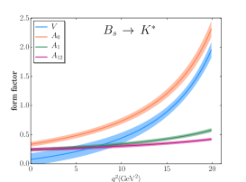
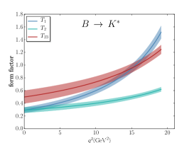
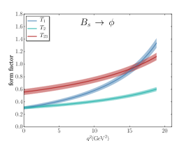
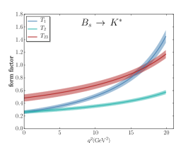
At two kinematic points the form factors are not all linearly independent. When , equations of motion may be used to relate matrix elements, giving two constraints on the form factors. At the kinematic endpoint, , two pairs of form factors become linearly dependent:
| (4) |
In our published work fits were done to individual form factors separately, with the exception of a joint fit to and , so that the constraint could be implemented. This was the most important constraint for existing measurements such as . In these proceedings we implement all constraints in (4) by performing simultaneous fits to the vector and axial vector form factors and to the tensor and pseudotensor form factors . This will ensure that endpoint relations such as are precisely satisfied [13]. The constraints are implemented by adding a fake “data point” to the fit requiring that the left-hand and right-hand sides (in the physical mass limit) are equal up to some uncertainty. For this uncertainty is set to be , an estimate for the size of terms truncated from our fit ansatz. For we take the uncertainty to be since we have data in the high- range. In practice, results do not change if either of these is reduced.
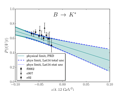
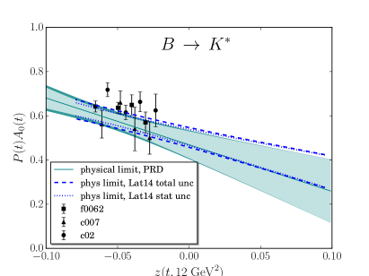
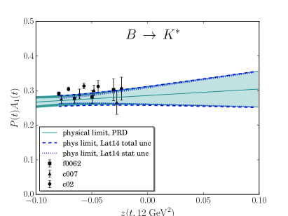
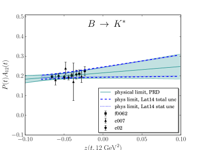
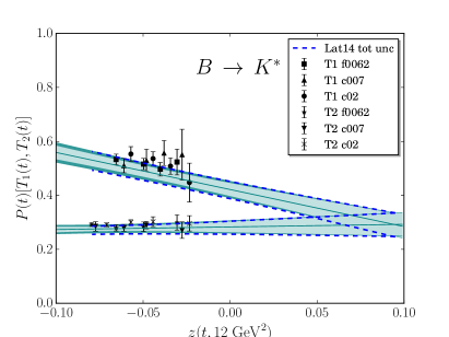
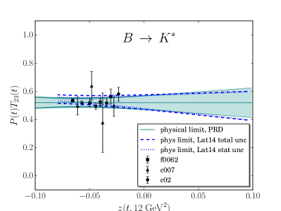
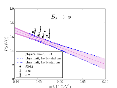
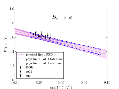
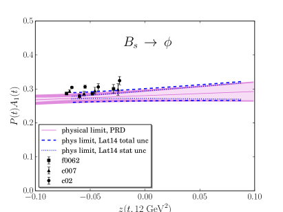
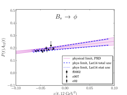
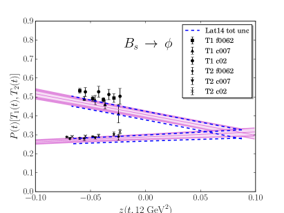
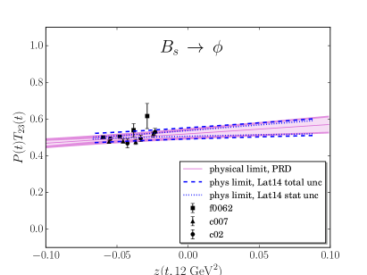
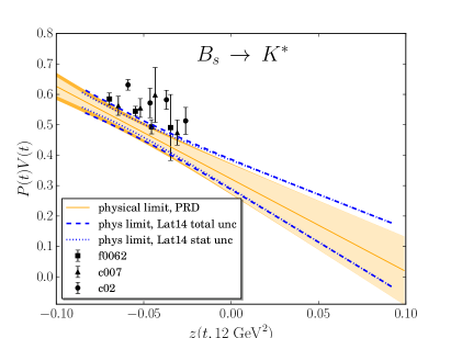
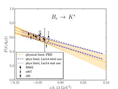
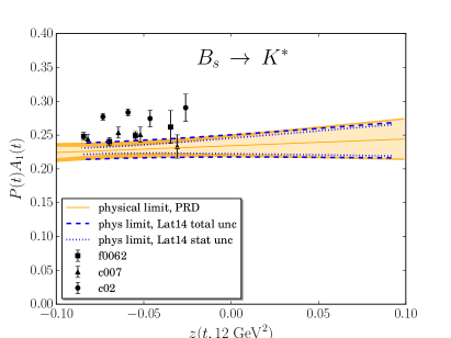
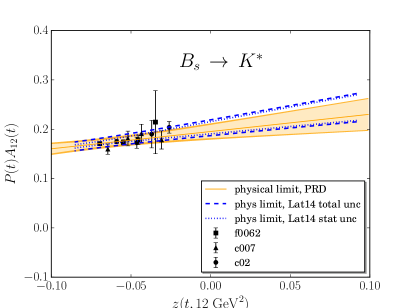
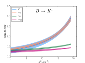
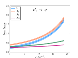
We have tried including cross-correlations between all of the form factor data in order to estimate the correlations between the full set of fit parameters. The data covariance matrix was not determined well enough to allow for a single fit, so several fits to sets of 3 or 4 form factors were done. We suspect that the data covariance matrices were still not entirely well-determined. For example, when we included cross-correlations but no new kinematic constraints compared to our published fits, we found deviations of approximately 1 standard deviation, despite the fact that the fit parameters were independent of each other. Therefore, for our final fit we include only the data correlations between and and between and . These are the pairs of form factors which must satisfy kinematic constraints (4) at . Figure 1 shows the results for the form factors in the physical limit. Further details and results of these fits are appended to the end of the arXiv version of this write-up [arXiv:1501.00367].
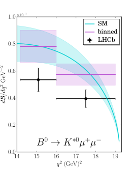
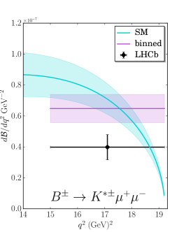
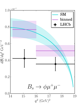
We use these new form factor fits, including the constraints (4) and the estimated correlation matrix, to determine several , , and observables. For most quantities, notably the differential branching fraction, we find only negligible changes to our published results fits [2]. Fig. 2 shows our Standard Model differential branching fraction compared to experimental data, with the data consistently lower than the theoretical prediction (see also Table 1). Tables 2 and 3 give Standard Model predictions for angular observables. The most significant change compared to [2] is to , which shifts and is more precisely determined. This is due to the inclusion of the constraint. There is also a shift in the central value of in the case of .
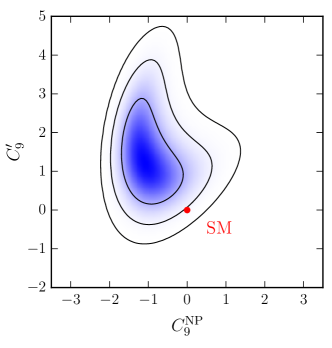
We have repeated our beyond-the-Standard-Model fit to large- experimental data for and , allowing the Wilson coefficients and to deviate from their Standard Model values (). This yields and , comparable to what we found before [2]. Figure 3 shows a contour plot of the likelihood function of this fit.
| bin (GeV2) | |||
|---|---|---|---|
| bin (GeV2) | |||||
|---|---|---|---|---|---|
| 0.360(42) | 0.410(35) | 0.612(17) | |||
| 0.336(25) | 0.347(21) | 0.650(08) | |||
| 0.347(32) | 0.375(26) | 0.633(12) |
| bin (GeV2) | |||
|---|---|---|---|
| 0.382(20) | 0.624(8) | ||
| 0.347(12) | 0.659(4) | ||
| 0.364(15) | 0.642(5) |
4 Open issues
One uncontrolled approximation in our calculation is that we fit correlation functions using a single interpolating operator for the vector meson final state, assuming that it corresponds to the or . A fully controlled calculation would include scattering states in the analysis. In order to do so, a much more expensive and complicated set of calculations must be undertaken. The path forward was set out in a paper which appeared during this conference [14]. Work to study the spectrum of and states has recently begun [15, 16, 17], marking the first major step toward a full lattice calculation of matrix elements. In the interim, the use of our form factor results comes with the assumption that threshold effects will be small. One might expect them to be smaller for than for since the is relatively narrow. One might also note that heavy meson chiral perturbation theory predicts percent-level threshold effects in form factors [18, 19] and hope that such is the case for lighter-mass mesons. Nevertheless at least there is a plan to systematically include this effect in the future.
Perhaps a larger open question regards the extent to which form factors are sufficient to determine the hadronic contributions to observables. In addition to matrix elements of 2-quark operators (2), there are matrix elements of non-local operators , notably where is a 4-quark operator which creates a pair, annihilated at another point by the vector current . It was expected that these matrix elements would make theoretical predictions unreliable for or . Within the context of an operator product expansion, leading-order contributions from these non-local operators can be (and, in our work, have been) included [20, 21]. However, contributions from the to the are larger than anticipated [22] and the same appears to be true for decays to vector mesons. Understanding nonfactorizable contributions is probably the most important open issue which theoretical predictions must confront [23].
5 Conclusions
This write-up summarizes our recent calculation of , , and form factors. Here we give a slightly improved set of fits to the form factor shapes, including all four kinematic constraints and estimates of the more significant correlations between form factor parameters. Given that this update is only a minor improvement upon our published work and has a small effect on observables, we would be grateful if those authors using the form factor results presented here would cite Ref. [1] in addition to this work.
Acknowledgments
We are grateful to R. Zwicky for discussions about the form factor fits and to the MILC Collaboration for making their gauge-field configurations publicly available. This work was supported in part by the STFC (UK), the DoE (US), and NSFC (China).
References
- [1] R. R. Horgan, Z. Liu, S. Meinel, and M. Wingate, Phys. Rev. D 89, 094501 (2014), arXiv:1310.3722.
- [2] R. R. Horgan, Z. Liu, S. Meinel, and M. Wingate, Phys. Rev. Lett. 112, 212003 (2014), arXiv:1310.3887.
- [3] LHCb Collaboration, R. Aaij et al., J. High Energy Phys. 08, 131 (2013), arXiv:1304.6325.
- [4] ATLAS Collaboration, (2013), ATLAS-CONF-2013-038, ATLAS-COM-CONF-2013-043.
- [5] LHCb Collaboration, R. Aaij et al., J. High Energy Phys. 07, 084 (2013), arXiv:1305.2168.
- [6] LHCb collaboration, R. Aaij et al., J. High Energy Phys. 06, 133 (2014), arXiv:1403.8044.
- [7] S. Descotes-Genon, J. Matias, and J. Virto, Phys. Rev. D 88, 074002 (2013), arXiv:1307.5683.
- [8] W. Altmannshofer and D. M. Straub, Eur. Phys. J. C 73, 2646 (2013), arXiv:1308.1501.
- [9] C. Hambrock, G. Hiller, S. Schacht, and R. Zwicky, Phys. Rev. D 89, 074014 (2014), arXiv:1308.4379.
- [10] F. Beaujean, C. Bobeth, and D. van Dyk, Eur. Phys. J. C 74, 2897 (2014), arXiv:1310.2478.
- [11] T. Hurth, F. Mahmoudi, and S. Neshatpour, J. High Energy Phys. 12, 053 (2014), arXiv:1410.4545.
- [12] W. Altmannshofer and D. M. Straub, (2014), arXiv:1411.3161.
- [13] G. Hiller and R. Zwicky, J. High Energy Phys. 03, 042 (2014), arXiv:1312.1923.
- [14] R. A. Briceño, M. T. Hansen, and A. Walker-Loud, Phys. Rev. D 91, 034501 (2015), arXiv:1406.5965.
- [15] S. Prelovsek, L. Leskovec, C. Lang, and D. Mohler, Phys. Rev. D 88, 054508 (2013), arXiv:1307.0736.
- [16] J. J. Dudek, R. G. Edwards, C. E. Thomas, and D. J. Wilson, Phys. Rev. Lett. 113, 182001 (2014), arXiv:1406.4158.
- [17] D. J. Wilson, J. J. Dudek, R. G. Edwards, and C. E. Thomas, Phys. Rev. D 91, 054008 (2015), arXiv:1411.2004.
- [18] L. Randall and M. B. Wise, Phys. Lett. B 303, 135 (1993), arXiv:hep-ph/9212315.
- [19] S. Hashimoto, A. S. Kronfeld, P. B. Mackenzie, S. M. Ryan, and J. N. Simone, Phys. Rev. D 66, 014503 (2002), arXiv:hep-ph/0110253.
- [20] B. Grinstein and D. Pirjol, Phys. Rev. D 70, 114005 (2004), arXiv:hep-ph/0404250.
- [21] M. Beylich, G. Buchalla, and T. Feldmann, Eur. Phys. J. C 71, 1635 (2011), arXiv:1101.5118.
- [22] LHCb Collaboration, R. Aaij et al., Phys. Rev. Lett. 111, 112003 (2013), arXiv:1307.7595.
- [23] J. Lyon and R. Zwicky, (2014), arXiv:1406.0566.
Appendix A Supplemental material
In this Appendix we give detailed tables in order for readers to use our new fits to reconstruct the form factors (in the physical limit). We also compare the new fits to the published ones [1].
Table 4 gives the mass differences between the or and the resonance (or effective pole) relevant for the various form factors. These enter the prefactor of the form factor shape (3). The remaining tables give results for the constant and linear coefficients ( and ) of in the form factor shape (3): Tables 5 and 6 for decays and Tables 7 and 8 for decays. In Tables 9 and 10 we give results for decays, such as the decay and the decay . These fit results come from separate fits for each Table, with correlations included only between and and between and . Other data correlations were not included for reasons discussed in Sec. 3.111ArXiv version 1 of this write-up gave an estimate of the full correlation matrix using fits to subsets of form factors. However, the resulting matrix was not positive semi-definite. One could devise a method for removing the negative eigenvalues, but since the differences between the fits given in versions 1 and 2 of these proceedings are not significant compared to other uncertainties, we believe the neglected correlations are presently insignificant.
Those wishing to use our form factor calculations for predictions of observables need not include all the correlation data. Large observables predominantly depend on and , and their fit parameters are not very correlated. On the other hand, the parameters for individual form factors, and , are highly correlated, so the uncertainty of the LQCD-determined form factor [Eq. (3)] is given (in the physical limit) by
| (5) |
Since physical results are obtained by setting in (3), one does not need our results for or except to look at the quark-mass dependence of the form factors. Data files containing the fit results as tabulated in Tables 5-10 are included as ancillary files with the arXiv submission.
| Form factor | |||
|---|---|---|---|
| , | |||
| , , , |
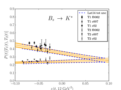
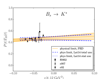
Figures 4, 5, and 6 show the fit results presented here compared to our published results [1]. The most visible difference in the Figures is the reduction of uncertainty in at low values of (positive ) due to the constraint that it equals at up to a known multiplicative factor. The inclusion of the constraints ensures endpoint relations are accurately satisfied [13]. Together these improvements to the fits yield slightly more precise and accurate predictions for several observables. Table 11 gives values for each of the form factors at a few reference kinematic points.
| value | ||||||||
|---|---|---|---|---|---|---|---|---|
| value | ||||||
|---|---|---|---|---|---|---|
| value | ||||||||
|---|---|---|---|---|---|---|---|---|
| value | ||||||
|---|---|---|---|---|---|---|
| value | ||||||||
|---|---|---|---|---|---|---|---|---|
| value | ||||||
|---|---|---|---|---|---|---|
| 0.620(35) | 0.444(25) | 0.623(35) | |||||
| 16 | 0.523(36) | 0.389(30) | 0.520(33) | ||||
| 12 | 0.440(42) | 0.339(40) | 0.433(37) | ||||
| 0 | 0.303(51) | 0.251(53) | 0.291(44) | ||||
| 0.624(32) | 0.396(21) | 0.605(31) | |||||
| 16 | 0.529(29) | 0.359(20) | 0.521(27) | ||||
| 12 | 0.439(28) | 0.321(22) | 0.439(25) | ||||
| 0 | 0.294(28) | 0.248(26) | 0.305(22) | ||||
| 0.582(32) | 0.424(23) | 0.578(31) | |||||
| 16 | 0.451(26) | 0.363(22) | 0.459(26) | ||||
| 12 | 0.370(26) | 0.321(25) | 0.383(25) | ||||
| 0 | 0.242(26) | 0.243(29) | 0.261(25) | ||||
