Impurity-induced gap system as a quantum data bus for quantum state transfer

Abstract

We introduce a tight-binding chain with a single impurity to act as a quantum data bus for perfect quantum state transfer. Our proposal is based on the weak coupling limit of the two outermost quantum dots to the data bus. First show that the data bus has an energy gap between the ground and first-excited states in the single-particle case induced by the impurity in the single particle case. By connecting two quantum dots to two sites of the data bus, the system can accomplish a high-fidelity and long-distance quantum state transfer. Numerical simulations were performed for a finite system; the results show that the numerical and analytical results of the effective coupling strength agree well with each other. Moreover, we study the robustness of this quantum communication protocol in the presence of disorder in the couplings between the nearest-neighbor quantum dots. We find that the gap of the system plays an important role in robust quantum state transfer.

I INTRODUCTION

The transfer of quantum states from one quantum unit of a quantum computer to another is of fundamental importance in quantum information science. Recently, in view of the great potential of a physical realization of the quantum computer, attention is being paid to the problem of the transfer of quantum information in a solid-state system.

Recently, spin systems have been proposed as a quantum data bus for transferring information. In a pioneering study Bose , Bose showed that the simplest coupled spin chain with uniform nearest-neighbor (NN) couplings is able to act as a quantum channel, i.e., the spin system allows the transmission of an arbitrary quantum state with high fidelity from one end to the other. The advantages of this protocol are that no external control is required throughout the entire transfer process, the quantum state transfer (QST) is equivalent to the natural dynamical evolution of the time-independent Hamiltonian, and the system can be isolated from the environment to minimize decoherence. However, the drawback of this proposal is that the transfer quality decreases with the size of chain. One way to overcome this problem is to precisely modulate the couplings between NN spins throughout the quantum data bus, as suggested in Ref. MC so as to obtain perfect QST, which is independent of the chain length. This is possible because the eigenvalues of the system match the parity of the corresponding eigenstates, which is a sufficient condition for perfect QST Song ; ST ; LY2 . However, such an implementation requires precise control of the system, which is not desirable in an experiment. Another approach to achieving perfect QST is based on a gap quantum system Cirac ; LY1 ; HMX ; XH ; CB ; Lukin ; MB ; AW0 ; AW ; SP ; SL ; SWAP ; LB ; TJ ; QI ; Venuti3 ; Venuti2 . By weakly connecting the transmitting and receiving qubits to a gap system, the total system’s dynamics can be reduced to those of an effective two- or three-level system. In addition to the fact that no extra controls are required for communication, a key advantage of these methods is their robustness against parameter disorder, which comes from inevitable technological errors in the experimental implementation. Moreover, we notice that the systems with long-range inter-qubit interactions for perfect QST or creating entanglement are well developed as well Venuti1 ; Petrosyan ; YS ; Kay ; Bose3 .

In this paper, we introduce an impurity-induced gapped system (IGS), which is a tight-binding chain with on-site energy applied on a single quantum dot (QD), to act as a quantum channel. We demonstrate the existence of a nonvanishing energy gap between the ground and first-excited states in the single-particle case. We also investigate the QST using the IGS. It is found that at lower temperatures, the total Hamiltonian can be mapped to a three-level effective Hamiltonian whose energy levels are equally spaced and can be used to perform near-perfect QST. In the weak-coupling limit, the coupling constant of the effective Hamiltonian has an inverse relationship with the transfer distance. Moreover, we study the robustness of the state transfer against the static imperfections of the couplings, as discussed in Ref. AZ ; Chiara . The resulting distribution of the transfer fidelities reveals that chains with boundary states are more resilient to imperfections. This is reflected in more instances of high-fidelity transfer through the spin chain. Compared with previously proposed schemes, the advantage of our scheme is that it is simple and can be readily applied to experiments.

This paper is organized as follows: In Section II, the model IGS is set up and its spectrum is introduced. In Section III, our QST protocol is set up and the effective Hamiltonian, $H_{\text{eff}}$, is deduced using perturbation theory. The scheme for using the IGS to transfer a quantum state is discussed in Section IV. Finally, conclusions of these investigations are presented in Section V.

II MODEL OF QUANTUM COMMUNICATION

II.1 Quantum data bus

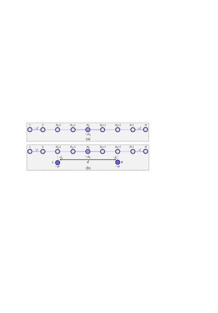
Figure 1: (Color online) (a) Schematic illustrations of impurity-induced gap system (IGS) which is a $N$-site chain with on-site energy applied on the central quantum dot. (b) A schematic setup for QST between two QDs L and R over the distance $d=2l+1$, through the gap system.

We begin by introducing a one-dimensional tight-binding chain of $N$ QDs with one diagonal impurity at $N_{0}$-th site, which acts as a quantum data bus. The model is shown in Fig. 1(a), which is described by the Hamiltonian

$$\hat{H}_{M}^{e}=-J\sum_{j=1}^{N-1}\sum_{\sigma=\uparrow,\downarrow}\left(\hat{c}_{j,\sigma}^{{\dagger}}\hat{c}_{j+1,\sigma}+\text{h.c.}\right)-\mu_{0}\sum_{\sigma=\uparrow,\downarrow}\hat{c}_{N_{0},\sigma}^{{\dagger}}\hat{c}_{N_{0},\sigma},$$ (1)

where $-J$ $(<0)$ is the hopping amplitude between NN sites $j$ and $j+1$, $\hat{c}_{j,\sigma}^{{\dagger}}$ and $\hat{c}_{j,\sigma}$ are the creation and annihilation operators of electrons on the $j$-th site with spin $\sigma$, and $-\mu_{0}$ $(<0)$ is the on-site energy of the defect. With a view toward the quantum information, we can encode the qubit on the spin state. Note that Eq. (1) does not contain any spin-spin interaction term; thus, the spin degree does not change during the evolution of the system. Hereafter, we shall omit the $\sigma$ index, denoting the electron operator with generic spin state as $\hat{a}_{j}^{{\dagger}}=\cos\theta\hat{c}_{j,\uparrow}^{\dagger}+e^{i\phi}\sin\theta\hat{c}_{j,\downarrow}^{\dagger}$. This system can be regarded as a spinless fermion system, and the feasibly obtained results can be applied to the original system. In this sense, we can concentrate on the spinless fermion model in the following discussion.

$$\hat{H}_{M}=-J\sum_{j=1}^{N-1}\left(\hat{a}_{j}^{{\dagger}}\hat{a}_{j+1}+\text{h.c.}\right)-\mu_{0}\hat{a}_{N_{0}}^{{\dagger}}\hat{a}_{N_{0}},$$ (2)

For the sake of clarity and simplicity, we only consider the case where the defect is placed in the middle of the medium, i.e., $N_{0}=(N+1)/2$. Note that the Hamiltonian, $\hat{H}_{M}$, commutes with the total number operator, $\hat{n}=\sum_{j=1}^{N}\hat{a}_{j}^{{\dagger}}\hat{a}_{j}$, and so the Hilbert space can be decomposed into subspaces corresponding to different particle numbers, $n$. For the case of transferring a single particle, we restrict the discussion to the single-particle subspace, which is spanned by the Fock states $\left|j\right\rangle=\hat{a}_{j}^{{\dagger}}\left|0\right\rangle$, with $j=1,2,...,N$.

In this study, we focus on the bound state (or the ground state of $\hat{H}_{M}$) of this Hamiltonian for nonzero $\mu_{0}$, which can be obtained via the Bethe ansatz method. We will also show that for Hamiltonian $\hat{H}_{M}$, there exists a finite energy gap, $\Delta=\varepsilon_{1}-\varepsilon_{g}\sim\mu_{0}^{2}/2J$, between the ground state and the first excited state.

To deduce the above conclusion, we write the state in the single-particle Hilbert space as $\left|\lambda_{n}\right\rangle=\sum_{j=1}^{N}f_{j}^{n}\left|j\right\rangle$. Substituting the discrete superposition state into the eigenequation $\hat{H}_{M}\left|\lambda_{n}\right\rangle=\varepsilon_{n}\left|\lambda_{n}\right\rangle$, we get

$$-J\sum_{i=1}^{N}\left(\delta_{i,j-1}+\delta_{i,j+1}\right)f_{i}^{n}=\left(\mu_{0}\delta_{j,N_{0}}+\varepsilon_{n}\right)f_{j}^{n},$$ (3)

with open boundary condition $f_{0}^{n}=f_{N+1}^{n}=0$.

For $\mu_{0}=0$, the solution of Eq. (3) is

$$f_{j}^{n}=\sqrt{\frac{1}{N_{0}}}\sin\left[\frac{(n+1)\pi j}{2N_{0}}\right],$$ (4)

with $n=0,$ $1,$ $2,\ldots,$ $N-1$, the eigenvalues are $\varepsilon_{n}=-2J\cos\left[(n+1)\pi/2N_{0}\right]$.

We now study the effect of the impurity on the energy spectrum of Hamiltonian $\hat{H}_{M}$ for nonzero $\mu_{0}$. Before making calculations, we make the following observations: first, when the Hamiltonian, $\hat{H}_{M}$, is processing mirror symmetry with respect to the inversion center, $N_{0}$, its eigenvectors, $\left|\lambda_{n}\right\rangle$, have definite parities. Moreover, if the eigenvalues, $\lambda_{n}$, are in increasing order, then the eigenvectors, $\left|\lambda_{n}\right\rangle$, change parity alternatively, i.e., the mirror-inverted eigenstates, $\left|\lambda_{n}\right\rangle$, satisfy the relation $f_{j}^{n}=(-1)^{n}f_{N+1-j}^{n}$ upon assuming that even (odd) $n$ label even (odd) eigenstates $\left|\lambda_{n}\right\rangle$. Second, the probability density of all the eigenstates with odd parity in the central site, $N_{0}$, is zero, i.e., $f_{N_{0}}^{2m-1}=0$, which means that the eigenstates with odd parity are unaffected by the presence of the impurity. Third, by the Hellmann-Feynman theorem, the eigenvalues of even-parity eigenstates decrease due to the presence of the impurity. Furthermore, the impurity contributes exactly one bound state, which we focus on in this study.

To see more precisely what happens for $\mu_{0}\neq 0$, we solve Eq. (3) via the Bethe Ansatz method. In this study, the bound state is the ground state of $\hat{H}_{M}$. Through a straightforward calculation, one can obtain the following analytical result for the ground state

$$f_{j}^{0}=\Omega^{-1/2}\times\left\{\begin{array}[]{c}\sinh k_{0}j,\text{ \ \ \ \ \ \ \ \ \ \ \ \ \ \ }j\leq N_{0}\\ \sinh k_{0}(N+1-j),\text{ }j>N_{0}\end{array}\right.,$$ (5)

with the eigenvalue $\lambda_{0}=-2J\sqrt{\xi^{2}+1}$, where $k_{0}=\ln\left[\xi+\sqrt{\xi^{2}+1}\right]$ and $\xi=\mu_{0}/2J$; $\Omega\approx e^{2k_{0}N_{0}}\left(e^{2k_{0}}+1\right)/4\left(e^{2k_{0}}-1\right)$ is the renormalization factor.

The remaining eigenstates with even parity are extended and similar to Eq. (4); the appropriate Ansatz is

$$f_{j}^{n}=\left\{\begin{array}[]{c}\sin k_{n}j,\text{ \ \ \ \ \ \ \ \ \ \ \ \ \ \ }j\leq N_{0}\\ \sin k_{n}(N+1-j),\text{ }j>N_{0}\end{array}\right.,$$ (6)

which yields the eigenvalue $\varepsilon_{n}=-2J\cos k_{n}$ and the wave vector, $k_{n}$, obeys

$$\xi\sin k_{n}N_{0}=\cos k_{n}N_{0}\sin k_{n}.$$ (7)

Setting $\tan\varphi_{n}=\xi/\sin k_{n}$, Eq. (7) becomes $\cos\left(k_{n}N_{0}+\varphi_{n}\right)=0$, whose allowed values are

$$k_{n}=\frac{\left(2m-1\right)\pi-2\varphi_{n}}{2N_{0}},m=1,2...,N_{0}-1.$$ (8)

From the above equations, we know that (i) the phase shift $\varphi_{n}=0$ for $\xi=0$ and $\varphi_{n}=\pi/2$ for $\xi=\infty$, and that (ii) the phase shifts do not alter the order of the sequence $\left\{k_{n}\right\}$.

Until now, we have only discussed the solutions of eigenequation $\hat{H}_{M}\left|\lambda_{n}\right\rangle=\varepsilon_{n}\left|\lambda_{n}\right\rangle$ without any external perturbation. In the thermodynamic limit where $N_{0}\rightarrow\infty$, the excited energies become a continuous energy band; it is not hard to find that the energy gap between the ground state and the first excited state (see the Fig. 2a) is

$$\Delta=2J\sqrt{\xi^{2}+1}-2J.$$ (9)

For very small values of onsite energy, i.e., $\mu_{0}\ll J$, we get $\Delta\approx J\xi^{2}$.

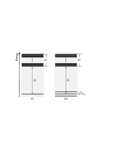
Figure 2: Schematic illustration of the energy levels of the system. (a) When the connections between two QDs and the medium switch off $J_{0}=0$ the ground states are three-fold degenerate. (b) When $J_{0}=0$ switches on, the degeneracy will be removed and split into three sub-levels with the level spacing $\delta=\sqrt{2}J_{\text{eff}}$. This is approximately equivalent to that of tight-binding chain with three QDs.

II.2 The subspace Hamiltonian

Now, let us introduce the protocol of quantum communication by using IGS, in which two individual QDs (sender and receiver) are symmetrically coupled to an IGS on opposite sides of the data bus (as illustrated in Fig. 1(b)). Moreover, QDs L and R are supplied with on-site energy, $-\mu$. The total Hamiltonian consisting of $(N+2)$ QDs reads

$$\hat{H} = \hat{H}_{0}+\hat{H}^{\prime},$$

$$\hat{H}_{0} = \hat{H}_{M}-\mu\left(\hat{a}_{L}^{{\dagger}}\hat{a}_{L}+\hat{a}_{R}^{{\dagger}}\hat{a}_{R}\right),$$

$$\hat{H}^{\prime} = -J_{0}\left(\hat{a}_{L}^{\dagger}\hat{a}_{N_{0}-l}+\hat{a}_{R}^{\dagger}\hat{a}_{N_{0}+l}+\text{h.c.}\right),$$ (10)

where $\hat{a}_{L}$ and $\hat{a}_{R}$ are the annihilation operators of electron on $L$ and $R$, $\left(N_{0}\pm l\right)$ denotes the connecting sites of the chain, and the coupling constant, $J_{0}$, measures the strength of the interaction.

In the absence of coupling between the two qubits and the medium ($J_{0}=0$) and setting $-\mu=\lambda_{0}$, the total Hamiltonian (10) can be diagonalized in the basis $\left\{\left|L\right\rangle,\left|R\right\rangle,\left|\lambda_{0}\right\rangle,\left|\lambda_{1}\right\rangle,\ldots,\left|\lambda_{N-1}\right\rangle\right\}$, and its ground states are threefold degenerate, i.e., $\left|L\right\rangle$, $\left|\lambda_{0}\right\rangle$, and $\left|R\right\rangle$ have the energy $E_{g}^{\left(0\right)}=-\mu$. These three states can be regarded as the components of an effective pseudo-spin-1 system that span an invariant subspace. The original energy degeneracy will break down by switching on the weak coupling, $J_{0}$ ($J_{0}\ll\Delta$), and the ground state will split into three sub-levels with level spacing $\Delta E=\sqrt{2}\left|J_{\text{eff}}\right|$, as illustrated in Fig. 2(b). Here, $J_{\text{eff}}$ is the effective hopping integral that can be calculated as follows.

When switching on $J_{0}$, the eigenequation becomes $(\hat{H}_{0}+\hat{H}^{\prime})\left|\psi\right\rangle=E\left|\psi\right\rangle$. For weak coupling between QDs and the bus, $J_{0}\ll\Delta$, $\hat{H}^{\prime}$ can be treated as a perturbation Hamiltonian. Let us assume that, in some definite way, we can divide the basis into two classes, $\left[G\right]=\left\{\left|L\right\rangle,\left|R\right\rangle,\left|\lambda_{0}\right\rangle\right\}$ where the relative complement of $\left[G\right]$ is denoted by $\left[O\right]=\left\{\left|\lambda_{1}\right\rangle,\ldots,\left|\lambda_{N-1}\right\rangle\right\}$. Defining

$$\mathcal{\hat{G}} = \left|L\right\rangle\left\langle L\right|+\left|\lambda_{0}\right\rangle\left\langle\lambda_{0}\right|+\left|R\right\rangle\left\langle R\right|,$$ (11)

$$\mathcal{\hat{O}} = \sum_{n=1}^{N-1}\left|\lambda_{n}\right\rangle\left\langle\lambda_{n}\right|,$$ (12)

denote two orthogonal projection operators of two different subspaces. It is easy to check that $\mathcal{\hat{G}\hat{O}}=0$ and satisfying $\mathcal{\hat{G}}+\mathcal{\hat{O}}=\mathbb{\hat{I}}$. The eigenequation can be rewritten as

$$\left(\mathcal{\hat{G}}+\mathcal{\hat{O}}\right)\hat{H}\left(\mathcal{\hat{G}}+\mathcal{\hat{O}}\right)\left(\mathcal{\hat{G}}+\mathcal{\hat{O}}\right)\left|\psi\right\rangle=E\left(\mathcal{\hat{G}}+\mathcal{\hat{O}}\right)\left|\psi\right\rangle.$$ (13)

The above equation can be decomposed into two basic formulae in subspaces $\left(G\right)$ and $\left(O\right)$

$$\hat{H}_{\mathcal{GG}}\mathcal{\hat{G}}\left|\psi\right\rangle+\hat{H}_{\mathcal{GO}}\mathcal{\hat{O}}\left|\psi\right\rangle = E\mathcal{\hat{G}}\left|\psi\right\rangle,$$ (14)

$$\hat{H}_{\mathcal{OG}}\mathcal{\hat{G}}\left|\psi\right\rangle+\hat{H}_{\mathcal{OO}}\mathcal{\hat{O}}\left|\psi\right\rangle = E\mathcal{\hat{O}}\left|\psi\right\rangle,$$ (15)

where $\hat{H}_{\alpha\beta}=\hat{\alpha}\hat{H}\hat{\beta}$, $\left(\hat{\alpha},\hat{\beta}=\mathcal{\hat{G}},\mathcal{\hat{O}}\right)$. Using Eq.  (15), one can express $\mathcal{\hat{O}}\left|\psi\right\rangle$ in terms of $\mathcal{\hat{G}}\left|\psi\right\rangle$:

$$\mathcal{\hat{O}}\left|\psi\right\rangle=\left(E-\hat{H}_{\mathcal{OO}}\right)^{-1}\hat{H}_{\mathcal{OG}}\mathcal{\hat{G}}\left|\psi\right\rangle,$$ (16)

so that, substituting the above equation into Eq. (14), one finds that, to second order, the equation only evolves $\mathcal{\hat{G}}\left|\psi\right\rangle$:

$$\hat{H}_{\text{eff}}\mathcal{\hat{G}}\left|\psi\right\rangle=E\mathcal{\hat{G}}\left|\psi\right\rangle,$$ (17)

where

$$\hat{H}_{\text{eff}}=\hat{H}_{\mathcal{GP}}+\hat{H}_{\mathcal{PO}}\left(E-\hat{H}_{\mathcal{OO}}\right)^{-1}\hat{H}_{\mathcal{OG}}$$ (18)

denotes the effectvie Hamiltonian in subspace $\left(A\right)$ with

$$\hat{H}_{\mathcal{GG}} = -J_{0}\zeta_{0}\left(\left|L\right\rangle+\left|R\right\rangle\right)\left\langle\lambda_{0}\right|+\text{h.c.}-\mu\mathcal{\hat{G}},$$ (19)

$$\hat{H}_{\mathcal{OO}} = \sum_{n=1}^{N-1}\lambda_{n}\left|\lambda_{n}\right\rangle\left\langle\lambda_{n}\right|,$$ (20)

$$\hat{H}_{\mathcal{GO}} = \sum_{n=1}^{N-1}-J_{0}\zeta_{n}\left(l\right)\left[\left|L\right\rangle+(-1)^{n}\left|R\right\rangle\right]\left\langle\lambda_{n}\right|.$$ (21)

and $\zeta_{n}\left(l\right)=\langle N_{0}-l\left|\lambda_{n}\right\rangle$. Through a straightforward calculation, one can obtain

$$\hat{H}_{\mathcal{GO}}\left(\mu+\hat{H}_{\mathcal{OO}}\right)^{-1}\hat{H}_{\mathcal{OG}}=\sum_{n=1}^{N-1}\frac{J_{0}^{2}\left|\zeta_{n}\right|^{2}}{E-\lambda_{n}}\left[\left|L\right\rangle+\left(-1\right)^{n}\left|R\right\rangle\right]\left[\left\langle L\right|+\left(-1\right)^{n}\left\langle R\right|\right].$$

Note that the eigenvalues, $E$, determined from Eq. (17), are perturbed eigenvalues around respective unperturbed value $-\mu$. With this connection, one seldom requires the second-order correction, which is small ($J_{0}^{2}\ll\left|E-\lambda_{n}\right|$, which is the condition for the perturbation procedure to be a good approximation in this problem); it is therefore sufficient to quote the first-order results

$$\hat{H}_{\text{eff}}\approx-J_{\text{eff}}\left(\left|L\right\rangle+\left|R\right\rangle\right)\left\langle\lambda_{0}\right|-\frac{\mu}{2}\left(\left|L\right\rangle\left\langle L\right|+\left|\lambda_{0}\right\rangle\left\langle\lambda_{0}\right|+\left|R\right\rangle\left\langle R\right|\right)+\text{h.c.},$$ (22)

with effective coupling strength $J_{\text{eff}}=J_{0}\zeta_{0}\left(l\right)$.

In this section, we have shown that the total Hamiltonian (10) can be simplified to the effective Hamiltonian (22), due to a large gap (compared with coupling strength $J_{0}$) existing in the medium. This approximation holds when the energy splitting, $\sqrt{2}J_{\text{eff}}$, caused by the $\hat{H}_{\text{eff}}$ is smaller than the typical gap for the unperturbed Hamiltonian, $\hat{H}_{0}$, i.e., $J_{\text{eff}}\ll\Delta$. To check the range of validity of the above effective Hamiltonian, we compare the analytical result of $J_{\text{eff}}$ with the results $\left(E_{1}-E_{0}\right)/\sqrt{2}$ obtained by direct numerical diagonalization of the Hamiltonian (10). The results of this comparison are plotted in Fig. 3 for a system of $N=499$, with $J_{0}=0.001J$, and $\mu_{0}=0.1J$, $0.05J$, and $0.01J$. In this figure, one can see that taking $\mu_{0}/J_{0}\$bigger than $50$, the effective coupling strength, $J_{\text{eff}}$, of $\hat{H}_{\text{eff}}$ agrees very well with that obtained numerically. So far, the validity of the effective Hamiltonian (22) is firmly established. Thus one should be able to obtain high-fidelity QST with the effective Hamiltonian whenever the perturbation solution is valid. Furthermore, we will show that the existence of an energy gap can also be used to protect the performance of QST in the presence of static disorder in the couplings of the quantum data bus.

However, it is worth pointing out that large $\mu_{0}$ can improve the validity of $\hat{H}_{\text{eff}}$ but decrease the transfer efficiency characterized by $J_{\text{eff}}$, since $1/J_{\text{eff}}$ determines the transfer time of the QST between the two qubits, L and R. As observed in Fig. 3, the decay rate of $J_{\text{eff}}$ directly depends on the value of $\mu_{0}$. The smaller the $\mu_{0}$ is, the slower the decay rate will be. Typically, $J_{\text{eff}}$ decreases almost linearly with the increase of the transfer distance for $\mu_{0}=0.01J$. From the two competing aspects described above, we can summarize the proper choice of the system parameters, $\mu_{0}$ and $J_{0}$, for high-fidelity QST.

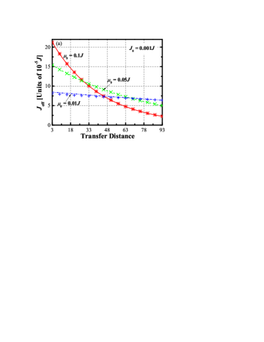
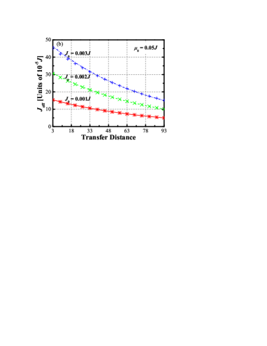
Figure 3: (Color online) (a) Behavior of $J_{\text{eff}}$ as a function of the transfer distance $d$ for a chain of $N=499$ sites, $J_{0}=0.001$ and different values of $\mu_{0}$. Curves from top to bottom are, respectively, for $\mu_{0}=0.1J$, $0.05J$, and $0.01J$. Continuous curves display the approximate expression for the $J_{\text{eff}}$ and symbols denote the exact numerical data which is given by $\left(E_{1}-E_{g}\right)/\sqrt{2}$. (b) The same as in (a) but for $\mu_{0}=0.05J$ and different values of $J_{0}$.

To briefly summarize, we have theoretically and numerically studied $J_{\text{eff}}$ as a function of $d$ in a specific range of parameters. However, the obtained conclusion is based on the fact that the $\hat{H}_{\text{eff}}$ given by Eq. (22) is a valid approximation in the studied range. In the following discussion, the validity of $\hat{H}_{\text{eff}}$ is investigated by comparing the eigenstates of $\hat{H}_{\text{eff}}$ with the lowest three states of the total system (10).

Define the quasi-angular momentum states $\left|j,m\right\rangle$ as

$$\left|1,0\right\rangle = \frac{1}{\sqrt{2}}\left(\left|L\right\rangle-\left|R\right\rangle\right),$$ (23)

$$\left|1,\pm 1\right\rangle = \frac{1}{2}\left(\left|L\right\rangle\pm\sqrt{2}\left|\lambda_{0}\right\rangle+\left|R\right\rangle\right),$$ (24)

which are the eigenstates of effective Hamiltonian (22). On the other hand, the eigenstates of $\hat{H}$ can be generally written as

$$\left|\psi_{jm}\right\rangle=c_{L}\left|L\right\rangle+\sum_{n=0}^{N-1}c_{n}\left|\lambda_{n}\right\rangle+c_{R}\left|R\right\rangle,$$ (25)

where we have the condition $\left|c_{L}\right|^{2}+\sum_{n}\left|c_{n}\right|^{2}+\left|c_{R}\right|^{2}=1$ for the normalization of $\left|\psi_{jm}\right\rangle$. Moreover, we assign the state $\left|\psi_{jm}\right\rangle$ to denote the ground state for $j=1$, $m=1$, the first excited state for $j=1$, $m=0$, and the second excited state for $j=1$, $m=-1$. To evaluate the fidelity of the $\hat{H}_{\text{eff}}$ induced by the perturbation, we introduce the overlap

$$P_{jm}=\left|\left\langle j,m\right.\left|\psi_{jm}\right\rangle\right|^{2}.$$ (26)

For the case where $J_{0}=0$, the ground states $\left|\psi_{jm}\right\rangle$ of $\hat{H}$ are threefold degenerate and $\left|\psi_{jm}\right\rangle$ can be written in symmetrical form by linear combinations of $\left|L\right\rangle$, $\left|\lambda_{0}\right\rangle$, and $\left|R\right\rangle$. Under this condition, one can obtain $P_{jm}=1$ for $j=1$ and $m=0$, $\pm 1$. In particular, we have $\left|c_{L}\right|^{2}=\left|c_{R}\right|^{2}=1/4$, $\left|c_{0}\right|^{2}=1/2$ for $m=\pm 1$ and $\left|c_{L}\right|^{2}=\left|c_{R}\right|^{2}=1/2$, $\left|c_{0}\right|^{2}=0$ for $m=0$. For the practical Hamiltonian $\hat{H}$, i.e., $J_{0}\neq 0$, the values of $\left|c_{i}\right|^{2}$ $\left(i=L,0,R\right)$ and $P_{jm}$ are numerically calculated for the three lowest eigenstates in the $N=499$ system with $\mu_{0}=0.1J$, $0.05J$ and $J_{0}=2\times 10^{-3}J$ for finite transfer distances $d=5$, , $15$, $25$, $35$, $45$, $55$, and $65$, which are listed in Tables I(a) and (b).

Table 1: The overlap $P_{jm}$ and its three components, which provide a criteria for the validity of $H_{\text{eff}}$, are calculated numerically for the ground state, first excited state and second excited state of total system for finite transfer distance $d=5$, $15$, $25$, $35$, $45$, $55$, and $65$. The results for $\mu_{0}=0.1J$, and $0.05J$ ($J_{0}=2\times 10^{-3}J$) are listed in (a), and (b) respectively. It shows that the result based on the realistic interaction is very close to that by $H_{\text{eff}}$ even if $\mu_{0}$ is not large enough.

States $\ j\$ $m$ $d=$   5     15    25     35     45    55    65 (a) $\left|c_{L}\right|^{2}$ 0.2552 0.2531 0.2539 0.2569 0.2618 0.2687 0.2778 $\left|\psi_{11}\right\rangle$ $1$ $1$ $\left|c_{0}\right|^{2}$ 0.4884 0.4932 0.4920 0.4860 0.4757 0.4613 0.4426 $\left|c_{R}\right|^{2}$ 0.2552 0.2531 0.2539 0.2569 0.2618 0.2687 0.2778 $P_{11}$ 0.9986 0.9994 0.9997 0.9995 0.9988 0.9973 0.9950 $\left|c_{L}\right|^{2}$ 0.4999 0.4994 0.4987 0.4980 0.4975 0.4971 0.4968 $\left|\psi_{10}\right\rangle$ $1$ $0$ $\left|c_{0}\right|^{2}$ 3.457$\times$10^-25 2.334$\times$10^-24 6.501$\times$10^-25 2.248$\times$10^-23 1.044$\times$10^-23 2.920$\times$10^-23 1.992$\times$10^-22 $\left|c_{R}\right|^{2}$ 0.4999 0.4994 0.4987 0.4980 0.4975 0.4971 0.4968 $P_{10}$ 0.9999 0.9988 0.9973 0.9960 0.9949 0.9941 0.9935 $\left|c_{L}\right|^{2}$ 0.2432 0.2462 0.2459 0.2429 0.2375 0.2301 0.2205 $\left|\psi_{1-1}\right\rangle$ $1$ $-1$ $\left|c_{0}\right|^{2}$ 0.5116 0.5068 0.5080 0.5140 0.5243 0.5387 0.5574 $\left|c_{R}\right|^{2}$ 0.2432 0.2462 0.2459 0.2429 0.2375 0.2301 0.2205 $P_{1-1}$ 0.9979 0.9992 0.9997 0.9995 0.9987 0.9973 0.9950 (b) $\left|c_{L}\right|^{2}$ 0.2641 0.2599 0.2580 0.2580 0.2595 0.2625 0.2666 $\left|\psi_{11}\right\rangle$ $1$ $1$ $\left|c_{0}\right|^{2}$ 0.4633 0.4741 0.4801 0.4817 0.4795 0.4738 0.4650 $\left|c_{R}\right|^{2}$ 0.2641 0.2599 0.2580 0.2580 0.2595 0.2625 0.2666 $P_{11}$ 0.9904 0.9933 0.9957 0.9973 0.9981 0.9980 0.9970 $\left|c_{L}\right|^{2}$ 0.4999 0.4985 0.4963 0.4937 0.4912 0.4887 0.4865 $\left|\psi_{10}\right\rangle$ $1$ $0$ $\left|c_{0}\right|^{2}$ 6.467$\times$10^-24 2.461$\times$10^-25 1.581$\times$10^-23 2.075$\times$10^-23 2.362$\times$10^-23 7.620$\times$10^-24 2.793$\times$10^-24 $\left|c_{R}\right|^{2}$ 0.4999 0.4985 0.4963 0.4937 0.4912 0.4887 0.4865 $P_{10}$ 0.9997 0.9970 0.9925 0.9875 0.9823 0.9774 0.9730 $\left|c_{L}\right|^{2}$ 0.2194 0.2286 0.2348 0.2379 0.2383 0.2360 0.2315 $\left|\psi_{1-1}\right\rangle$ $1$ $-1$ $\left|c_{0}\right|^{2}$ 0.5318 0.5231 0.5185 0.5177 0.5203 0.5261 0.5350 $\left|c_{R}\right|^{2}$ 0.2194 0.2286 0.2348 0.2379 0.2383 0.2360 0.2315 $P_{1-1}$ 0.9684 0.9791 0.9874 0.9931 0.9963 0.9974 0.9967

We remark that the condition for mapping $\hat{H}$ to the effective Hamiltonian (22) is that $J_{0}$ must be small enough compared to the energy gap $\Delta$ of the medium rather than the on-site energy $\mu_{0}$. As mentioned before, the energy gap is $\Delta\approx\mu_{0}^{2}/4J$ for small $\mu_{0}$ (compared with $J$). It is straightforward to obtain $\Delta\approx 2.5\times 10^{-3}J$ for $\mu_{0}=0.1J$ and $\Delta\approx 6.25\times 10^{-4}J$ for $\mu_{0}=0.05J$. From the numerical results shown in Table I, we observe that the realistic interaction leads to the results for $\left|c_{i}\right|^{2}$ $\left(i=L,0,R\right)$, which are very close to those described by $\hat{H}_{\text{eff}}$, even if $\Delta$ is of the same order of $J_{0}$. It is clear that such a three-level subsystem allows state $\left|L\right\rangle$ to transfer with high fidelity, and the coherent population exhibits oscillations between the QDs on the two ends. The oscillation period of the population is given by $\tau=\pi/\sqrt{2}J_{\text{eff}}$, and we can say that the quantum state is transferred from QD $L$ to QD $R$ at the time $\tau=\left(2n-1\right)\times\tau$.

III QUANTUM STATE TRANSFER

III.1 Weak Coupling Regime

Note that the spectrum structure and the corresponding parity of the effective Hamiltonian, $\hat{H}_{\text{eff}}$, obey the spectrum-parity matching condition (SPMC) ST ; LY2 exactly, which is the general criterion for perfect QST. In this section, we consider the QST scheme based on our system. Assume Alice is at the sender site, A, and Bob is at the receiver site, B. Let Alice hold an electron with a spin state that she wants to communicate to Bob of $\left|\varphi\right\rangle=\cos\left(\theta/2\right)\left|\uparrow\right\rangle+e^{i\phi}\sin\left(\theta/2\right)\left|\downarrow\right\rangle$, where $\left|\uparrow\right\rangle$ $\left(\left|\downarrow\right\rangle\right)$ denotes the spin-up (down) state. Thus, the initial state of the total system is $\left|\Psi\left(0\right)\right\rangle=\left|L\right\rangle=\left(\cos\theta c_{L,\uparrow}^{\dagger}+e^{i\phi}\sin\theta c_{L,\downarrow}^{\dagger}\right)\left|0\right\rangle_{L}$, which is a superposition of the eigenstates of Hamiltonian $\hat{H}_{\text{eff}}$

$$\left|\Psi\left(0\right)\right\rangle=\frac{1}{2}\left(\left|1,1\right\rangle+\sqrt{2}\left|1,0\right\rangle+\left|1,-1\right\rangle\right).$$ (27)

At time $t$, the initial state $\left|\Psi\left(0\right)\right\rangle$ evolves into

$$\left|\Psi\left(t\right)\right\rangle = e^{-i\hat{H}_{\text{eff}}t}\left|\Psi\left(0\right)\right\rangle$$ (28)

$$= \frac{1}{2}\left(e^{i\delta t}\left|1,1\right\rangle+\sqrt{2}\left|1,0\right\rangle+e^{-i\delta t}\left|1,-1\right\rangle\right)$$

where $\delta=\sqrt{2}J_{\text{eff}}$, and we have neglected the overall phase, $e^{-i\varepsilon_{g}^{(0)}t}$. The density matrix corresponding to $\left|\Psi\left(t\right)\right\rangle$ is $\rho=\left|\Psi\left(t\right)\right\rangle\left\langle\Psi\left(t\right)\right|$, and the probability of state $\left|\Psi\left(0\right)\right\rangle$ transferring to the QD R at time $t$ is defined as

$$F(t)=\text{Tr}(\rho\rho_{R})=\sin^{4}\left(\frac{\delta t}{2}\right).$$ (29)

At the moment when $t=\tau=\pi/\delta$, $F(\tau)=1$ indicates that our scheme can perform QST perfectly. That is to say, the system evolves into a new factorized state

$$\left|\Psi\left(\tau\right)\right\rangle = \frac{1}{2}\left(e^{i\pi}\left|1,1\right\rangle+\sqrt{2}\left|1,0\right\rangle+e^{-i\pi}\left|1,-1\right\rangle\right)$$ (30)

$$= e^{i\pi}\left|R\right\rangle.$$

As an example of verifying the validity of the effective Hamiltonian $\hat{H}_{\text{eff}}$, the fidelity for $N=499$ and transfer distance $d=5$, with $J_{0}=2\times 10^{-3}J$, and $\mu_{0}=0.1J$, $0.05J$ are plotted in Figs. 4(a) and (b). They show that small $J_{0}$ leads to a result for transfer fidelity, which is very close to that described by the effective Hamiltonian, $\hat{H}_{\text{eff}}$.

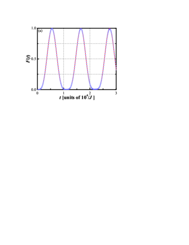
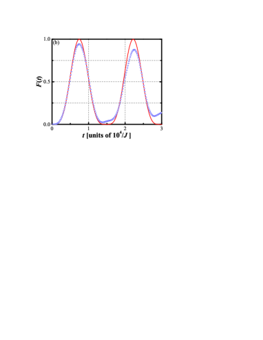
Figure 4: (Color online) Comparison of the exact transition probability $F(t)$ (open circle) with the analytic result of Eq. (27) (red solid line) for the system with $N=499$, $l=2$, $J_{0}=2\times 10^{-3}J$, $\mu_{0}=0.1J$ (upper plot), and $0.05J$ (lower plot). Time is expressed in units of $10^{4}/J$. It shows that, small $J_{0}$ leads to the result about transfer fidelity is very close to that described by the effective Hamiltonian $H_{\text{eff}}$.

III.2 Robustness to Disorder

We now turn to the performance of spin chains in the presence of static imperfections in the couplings, which are unavoidable in experimental implementations. We will show that the energy gap can protect the performance of the QST in the presence of static disorder in the system parameters.

We now assume that the tunnel coupling of the medium Hamiltonian has a random but constant offset, $\delta\epsilon_{j}$, i.e.,

$$\hat{H}^{\prime} = \sum_{j=1}^{N-1}-J(1+\delta\epsilon_{j})\left(\hat{a}_{j}^{{\dagger}}\hat{a}_{j+1}+\text{h.c.}\right)$$ (31)

$$-\mu_{0}\hat{a}_{N_{0}}^{{\dagger}}\hat{a}_{N_{0}}-\mu\left(\hat{a}_{L}^{{\dagger}}\hat{a}_{L}+\hat{a}_{R}^{{\dagger}}\hat{a}_{R}\right)-J_{0}\left(\hat{a}_{L}^{\dagger}\hat{a}_{N_{0}-l}+\hat{a}_{R}^{\dagger}\hat{a}_{N_{0}+l}+\text{h.c.}\right),$$

where $\delta$ is the maximum coupling offset bias relative to $J$; $\epsilon_{j}$ is drawn from the standard uniform distribution in the interval $\left[-1,1\right]$ and all $\epsilon_{j}$ are completely uncorrelated with all sites along the chain.

We numerically calculate the Schrödinger equation for the dynamical evolution and compute the overlap, $\mathcal{F}(t)=\left|\left\langle R\right|e^{-i\hat{H}^{\prime}t}\left|L\right\rangle\right|^{2}$, to assess the performance of the chain. In Fig. 5 we plot the behavior of $\mathcal{F}(t)$ as a function of time, $t$, in the system with $N=499$ QDs, $l=2$, $J_{0}=2\times 10^{-3}J$ for three cases: (a) $\mu_{0}=0.1J$, $\delta=5\times 10^{-3}$, (b) $\mu_{0}=0.1J$, $\delta=1\times 10^{-2}$, and (c) $\mu_{0}=0.5J$, $\delta=1\times 10^{-2}$. From this comparison, one can see that (i) this scheme is robust against the static disorders that would be unavoidable in experimental implementations and (ii) that the large energy gap (or large $\mu_{0}$) is more robust than small one against disorder.

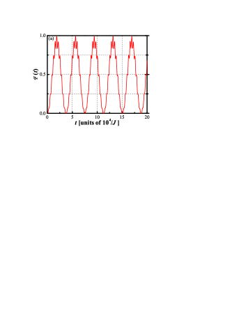
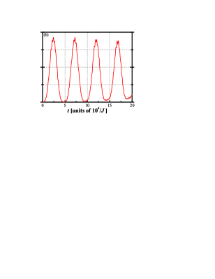
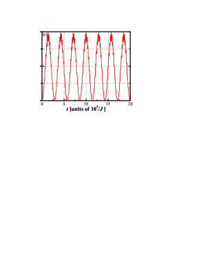
Figure 5: (Color online) The transition probability $F(t)$ of QST as a function of time in a $N=499$ system with $J_{0}=2\times 10^{-3}J$, $l=2$ and random imperfections of coupling strength $\delta$ function of time. The left figure corresponds to the case when $\mu_{0}=0.1J$ and $\delta=5\times 10^{-3}$, the middle figure to $\mu_{0}=0.1J$ and $\delta=1\times 10^{-2}$, and the right figure to $\mu_{0}=0.5J$ and $\delta=1\times 10^{-2}$. The results shows that weak fluctuations in the coupling strengths do not deteriorate the quality of QST due to the exitance of energy gap.

IV SUMMARY

According to quantum mechanics, it is not difficult to establish a long-distance QST using a gap system. However, the magnitude of the gap in this kind of scheme is crucial: first, the gap should be independent of the size of the system; second, the energy gap should be manipulated as required for perfect QST. The reason is that if the gap is too large, the QST period increases exponentially with the distance between two distant parities; when the gap is too small, the fidelity of the QST is reduced.

In this study, the quantum transmission of an electron through an IGS (serving as the data bus) is studied by theoretical analysis and numerical simulation. First, we show that the IGS has a nonvanishing energy gap above the ground state, which depends only on the on-site energy, $-\mu_{0}$, of the impurity. The approach to realize perfect QST is based on weakly connecting two external QDs with the bus. Different transfer distances can be achieved by suitable choices of connecting sites to the data bus. By treating the weak coupling as a perturbation, we find that a gap system can induce an effective three-level Hamiltonian [Eq. (22)]. This theoretical result is confirmed by performing numerical simulations; moreover, the effective coupling, $J_{\text{eff}}$, also decays slowly with increasing transfer distance if the system parameters are chosen reasonably.

Furthermore, the fault tolerance for more realistic system parameters is also demonstrated. It has been shown that perfect state transfer can also be achieved in the presence of disorder. For larger values of the energy gap (or $\mu_{0}$), the effect of disorder on the quality of QST will be strongly suppressed.

References

- (1) S. Bose, Phys. Rev. lett. 91, 207901 (2003); S. Bose, Contemporary Physics, 48 (1), 13-30 (2007).
- (2) M. Christandl, N. Datta, A. Ekert and A.J. Landahl, Phys. Rev. Lett. 92, 187902 (2004).
- (3) Z. Song and C. P. Sun, Low Temp. Phys. 31, 686 (2005).
- (4) T. Shi, Y. Li, Z. Song, and C.-P. Sun, Phys Rev A, 71, 032309 (2005).
- (5) Y. Li, Z. Song, and C.-P. Sun, Commun. Theor. Phys. 48, 445 (2007).
- (6) F. Verstraete, M. A. Martín-Delgado, and J. I. Cirac, Phys. Rev. Lett. 92, 087201 (2004).
- (7) Y. Li, T. Shi, B. Chen, Z. Song, and C.-P. Sun, Phys. Rev. A 71, 022301 (2005).
- (8) M.-X. Huo, Y. Li, Z. Song, and C.-P. Sun, Europhysics Letters 84, 30004 (2008).
- (9) Xiang Hao and Shiqun Zhu, Phys. Rev. A 78, 044302 (2008).
- (10) B. Chen, Z. Song, Sci. China Ser. G-Phys. Mech. Astron., 53, 1266 (2010).
- (11) N. Y. Yao, L. Jiang, A. V. Gorshkov et al, Phy. Rev. Lett. 106, 040505 (2011).
- (12) M. Bruderer, K. Franke, S. Ragg, W. Belzig, and D. Obreschkow, Phys. Rev. A 85, 022312 (2012).
- (13) A. Wójcik, T. Łuczak, P. Kurzyński, A. Grudka, T. Gdala, and M. Bednarska, Phys. Rev. A 72, 034303 (2005).
- (14) A. Wójcik, T. Łuczak, P. Kurzyński, A. Grudka, T. Gdala, and M. Bednarska, Phys. Rev. A 75, 022330 (2007).
- (15) S. Paganelli, S. Lorenzo, Tony J. G. Apollaro, F. Plastina, and Gian Luca Giorgi, Phys. Rev. A 87, 062309 (2013).
- (16) S. Lorenzo, T. J. G. Apollaro, A. Sindona, and F. Plastina, Phys. Rev. A 87, 042313 (2013).
- (17) B.-Q. Liu, L.-A. Wu, B. Shao, and J. Zou, Phys. Rev. A 85, 042328 (2012).
- (18) L. Banchi, T. J. G. Apollaro, A. Cuccoli, R. Vaia, and P. Verrucchi, New J. Phys, 13, 123006 (2011).
- (19) T. J. G. Apollaro, L. Banchi, A. Cuccoli, R. Vaia, and P. Verrucchi, Phys. Rev. A 85, 052319 (2012).
- (20) T. Linneweber, J. Stolze, and G. Uhrig, Int. J. Quant. Inf. 10, 1250029 (2012).
- (21) L. Campos Venuti, C. Degli Esposti Boschi, and M. Roncaglia, Phy. Rev. Lett. 99, 060401 (2007).
- (22) L. Campos Venuti, S. M. Giampaolo, F. Illuminati, and P. Zanardi, Phys. Rev. A 76, 052328 (2007).
- (23) L. Campos Venuti, C. Degli Esposti Boschi, and M. Roncaglia, Phy. Rev. Lett. 96(24), 247206 (2006).
- (24) D. Petrosyan, G. M. Nikolopoulos, and P. Lambropoulos, Phys. Rev. A 81, 042307 (2010).
- (25) S. Yang, Z. Song, and C.-P. Sun, Sci. China Ser. G-Phys. Mech. Astron., 51, 45 (2008).
- (26) A. Kay, Phys Rev A, 73, 032306 (2006).
- (27) M. Avellino, A. J. Fisher, and S. Bose, Phys. Rev. A 74, 012321 (2006).
- (28) A. Zwick, G. A. Álvarez, J. Stolze, and O. Osenda, Phys. Rev. A 84, 022311 (2011); ibid. 85, 012318 (2012).
- (29) Gabriele De Chiara, Davide Rossini, Simone Montangero, and Rosario Fazio, Phys. Rev. A 72, 012323 (2005).