Multi-Access Communications with Energy Harvesting: A Multi-Armed Bandit Model and the Optimality of the Myopic Policy

Abstract

A multi-access wireless network with $N$ transmitting nodes, each equipped with an energy harvesting (EH) device and a rechargeable battery of finite capacity, is studied. At each time slot (TS) a node is operative with a certain probability, which may depend on the availability of data, or the state of its channel. The energy arrival process at each node is modelled as an independent two-state Markov process, such that, at each TS, a node either harvests one unit of energy, or none. At each TS a subset of the nodes is scheduled by the access point (AP). The scheduling policy that maximises the total throughput is studied assuming that the AP does not know the states of either the EH processes or the batteries. The problem is identified as a restless multi-armed bandit (RMAB) problem, and an upper bound on the optimal scheduling policy is found. Under certain assumptions regarding the EH processes and the battery sizes, the optimality of the myopic policy (MP) is proven. For the general case, the performance of MP is compared numerically to the upper bound.

I Introduction

Low-power wireless networks, such as machine-to-machine and wireless sensor networks, can be complemented with energy harvesting (EH) technology to extend the network lifetime. A low-power wireless node has a limited lifetime constrained by the battery size; but when complemented with an EH device and a rechargeable battery, its lifetime can be prolonged significantly. However, energy availability at the EH nodes is scarce, and, due to the random nature of the energy sources, energy arrives at random times and in arbitrary amounts. Hence, in order to take the most out of the scarce energy, it is important to optimise the scheduling policy of the wireless network.

Previous research on EH wireless networks can be grouped into three, based on the information available regarding the random processes governing the system [1]. In the offline optimization framework, availability of non-causal information on the exact realizations of the random processes governing the system is assumed at the transmitter [2], [3]. In the online optimization framework [4, 5, 6, 7, 8, 9, 10, 11], the statistics governing the random processes are assumed to be available at the transmitter, and their realizations are known only causally. The EH communication system is modeled as a Markov decision process (MDP) [4], or as a partially observable MDP (POMDP) [5], and dynamic programming (DP) [12] can be used to optimise the EH communication system numerically. In many practical applications, the state space of the corresponding MDPs and POMDPs is large, and DP becomes computationally prohibitive [13], and the numerical results of DP do not provide much intuition about the structure of the optimal scheduling policy. In order to avoid complex numerical optimisations it is important to characterize the behaviour of the optimal scheduling policy and identify properties about its structure; however, this is possible only in some special cases [8, 9, 6]. In the learning optimization framework, the knowledge about the system behaviour is further relaxed, and even the statistical knowledge about the random processes governing the system is not assumed, and the optimal policy scheduling is learnt over time [11].

We study online scheduling of low-power wireless nodes by an access point (AP). The nodes are equipped with EH devices, and powered by rechargeable batteries. At each time slot (TS) a node is operative with a certain probability, which may depend on the channel conditions or the availability of data at the node. The EH process at each node is modelled as an independent Markov process, and at each TS, a node either harvests one unit of energy or does not harvest any. The AP is in charge of scheduling, at each TS, the EH nodes to the available orthogonal channels. A node transmits only when it is scheduled and is operative at the same time. Hence, at each TS the AP learns the EH process states and battery levels of the operative nodes that are scheduled, but does not receive any information about the other nodes. The AP is interested in maximising the expected sum throughput within a given time horizon. This problem can be model as a POMDP and solved numerically using DP at the expense of a high-computational cost. Instead, we model it as a restless multi-armed bandit (RMAB) problem [14], and prove the optimality of a low-complexity policy in two special cases. Moreover, by relaxing the constraint on the number of nodes that the AP can schedule at each TS, we obtain an upper bound on the performance of the optimal scheduling policy. Finally, the performance of the low complexity policy is compared to that of the upper bound numerically. The main technical contributions of the paper are summarised as follows:

• We show the optimality of a MP if the nodes do not harvest energy and transmit data at the same time, and the EH process is affected by the scheduling policy.

• We show the optimality of MP if the nodes do not have batteries and can transmit only if they have harvested energy in the previous TS.

• We provide an upper bound on the performance for the general case by relaxing the constraint on the number of nodes that can be scheduled at each TS.

• We show numerically that MP performs close to the upper bound for the general case.

The rest of this paper is organized as follows. Section II is dedicated to a summary of the related literature. In Section III, we present the EH wireless multi-access network model. In Sections IV and V we characterize explicitly the structure of the optimal policy that maximises the sum throughput for two special cases. In Section VI, we provide an upper bound on the performance. Finally, in Section VII we compare the performance of MP with that of the upperbound through numerical analysis. Section VIII concludes the paper.

II Related Work

There is a growing research interest in EH wireless communication systems, and in particular, in developing scheduling policies that exploit the scarce harvested energy in the most efficient manner. In large EH wireless networks, since numerical optimization is computationally prohibitive, it is important to characterise the optimal scheduling policy explicitly, or certain properties of it.

In [6], the authors assume that the data packets arrive at the EH transmitter as a Poisson process, and each packet has an intrinsic value assigned to it, which also is a random variable. The optimal transmission policy that maximizes the average value of the received packets at the destination is proven to be a threshold policy. However, the values of the thresholds have to be computed using numerical techniques, such as DP or linear programming (LP). Reference [7] extends the problem in [6] to the multi-access scenario.

Multi-access in EH wireless networks with a central scheduler, static channels and backlogged nodes has been studied in [8, 9, 10]. The central scheduler in [8] does not know the battery levels or the states of the EH processes at the nodes. Assuming that the nodes have unit size batteries, the system is modeled as an RMAB, and MP, which has a round robin (RR) structure, is shown to maximise the sum throughput. Reference [9] considers nodes with batteries of arbitrary capacity, and MP is found to be optimal in two special cases. In contrast to the present paper, [9] considers static channels and backlogged nodes, and the optimality proof exploits the RR structure of MP. In [10], considering infinite-capacity batteries, an asymptotically optimal policy is proposed.

The problem studied in this paper is modeled as an RMAB problem. In the classic RMAB problem there are several arms, each of which is modelled as a Markov chain [14]. The states of the arms are unknown, and at each TS an arm is played. The played arm reveals its state and yields a reward, which is a function of the state. The objective is to find a policy that maximises the total reward over time. RMAB problems have been shown to be, in general, PSPACE hard [15], and our knowledge on the structure of the optimal policy for general RMAB problem is limited.

Recently, the RMAB model has been used to study channel access and cognitive radio problems, and new results on the optimality of MP have been obtained [16, 17, 18, 19, 20]. The structure and the optimality of MP is proven in [16] and [17] for single and multiple plays, respectively, under certain conditions on the Markov transition probabilities. In [18] the optimality of MP is shown for a general class of monotone affine reward functions, which include arms with arbitrary number of states. The optimality of MP is proven in [19] when the arms’ states follow non-identical Markov chains. The case of imperfect channel detection is studied in [20], and MP is found to be optimal when the false alarm probability of the channel state detector is below a certain value.

III System Model

We consider an EH wireless network with $N$ EH nodes and one AP, as depicted in Figure 1. Time is divided into TSs of constant duration, and the AP is in charge of scheduling $K$ of the $N$ nodes to the $K$ available orthogonal channels at each TS. A node is operative at each TS with a fixed probability $p$ independent over TSs and nodes, and inoperative otherwise. We consider that a node is in the operative state if it has a data packet to transmit in its buffer and its channel to the AP is in a good state, while it is inoperative otherwise even if it is scheduled to a channel. The EH process is modelled as a Markov chain, which can be either in the harvesting or in the non-harvesting state, denoted by states $1$ and $0$, respectively. We denote by $p_{ij}$ the transition probability from state $i$ to $j$, and assume that $p_{11}\geq p_{01}$, that is, the EH process is positively correlated in time, and hence, if the EH process is in state $i$, it is more likely to remain in state $i$ than switching to the other state. We denote by $E^{s}_{i}(n)$ and $E^{h}_{i}(n)$ the state of the EH process and the amount of energy harvested by node $i$, respectively, in TS $n$. The energy harvested in TS $n$ is available for transmission in TS $n+1$. We assume that one fundamental unit of energy is harvested when the Markov process makes a transition to the harvesting state, that is, $E_{i}^{h}(n)=E_{i}^{s}(n+1)$. Each node is equipped with a battery of capacity $B$, and we denote by $B_{i}(n)\in\{0,\ldots,B\}$ the amount of energy stored in the battery of node $i$ at the beginning of TS $n$. The state of node $i$ in TS $n$, $S_{i}(n)$, is given by its battery and EH process states, $S_{i}(n)=(E^{s}_{i}(n),B_{i}(n))\in\{0,1\}\times\{0,\ldots,B\}$. The system state is characterized by the joint states of all the nodes.

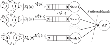
Figure 1: System model with $N$ EH nodes with finite size batteries and $K$ orthogonal channels.

The system functions as follows: At the beginning of each TS, the AP schedules $K$ out of $N$ nodes, such that a single node is allocated to each orthogonal channel. When a node is scheduled, if it is operative in that TS, i.e., it has data to transmit and its channel is in a good state, it transmits a data packet as well as the current state of its EH process to the AP. If it is not operative it transmits a status beacon to the AP, and backs off. We say that a node is active in a TS if it is scheduled by the AP and is operative; and hence, it transmits a data packet to the AP, otherwise we say that the node is idle in this TS, that is, the node is not scheduled or it is scheduled, but it is not operative. We denote by $\mathcal{K}(n)$ and $\mathcal{K}^{a}(n)$ the set of nodes scheduled by the AP, and the set of active nodes in TS $n$, respectively, where $\mathcal{K}^{a}(n)\subseteq\mathcal{K}(n)$.

We assume that the transmission rate is a linear function of the transmit power, which is an accurate approximation in the low power regime. When the power-rate function is linear, the total number of bits transmitted to the AP is maximised when an active node transmits at a constant power throughout the TS, using all its energy. To simplify the notation we normalise the power-rate function such that the number of bits transmitted within a TS is equal to the energy used for transmission. Then the expected throughput in TS $n$ is

$$R(\mathcal{K}(n))=\mathds{E}\left[\leavevmode\nobreak\ \leavevmode\nobreak\ \sum_{\mathclap{i\in\mathcal{K}^{a}(n)}}B_{i}(n)\right]=p\sum_{\mathclap{i\in\mathcal{K}(n)}}B_{i}(n).$$ (1)

The objective of the AP is to schedule the best set of nodes, $\mathcal{K}(n)$, at each TS in order to maximize (1), without knowing which nodes are operative, the battery levels, or the EH states. The only information the AP receives is the EH state of the active nodes at each TS. Note that the AP also knows the battery state of the active nodes after transmission since they use all their energy.

A scheduling policy is an algorithm that schedules nodes at each TS $n$, based on the previous observations of the EH states and battery levels. The objective of the AP is to find the scheduling policy $\mathcal{K}(n)$, $\forall n\in[1,T]$, that maximizes the total discounted throughput, given by

$$\max_{\{\mathcal{K}(n)\}_{n=1}^{T}} \leavevmode\nobreak\ \leavevmode\nobreak\ \sum_{n=1}^{T}\beta^{n-1}R(\mathcal{K}(n)),$$ (2)

s.t. $$B_{i}(n+1)=\min\{B_{i}(n)$$

$$+E^{h}_{i}(n),B\}\cdot\mathds{1}_{i\notin\mathcal{K}^{a}(n)}+E^{h}_{i}(n)\cdot\mathds{1}_{i\in\mathcal{K}^{a}(n)},$$

where $0<\beta\leq 1$ is the discount factor, and $\mathds{1}_{a}$ is the indicator function, defined as $\mathds{1}_{a}=1$ if $a$ is true, and $\mathds{1}_{a}=0$, otherwise.

If the AP is informed on the current state of all the nodes at each TS, the problem would be formulated as an MDP, and solved using LP or DP [12]. However, in practice transmitting all the nodes’ states to the AP introduces further overhead and energy consumption; and hence, is not considered here. Accordingly, the appropriate model for our problem is a POMDP. It can be shown that a sufficient statistic for optimal decision making in a POMDP is given by the conditional probability of the system states given all the past actions and observations, which, in our problem, depends only on the number of TSs each node has been idle for, and on the realisation of each node’s EH state last time it was active. Hence, we can reformulate the POMDP into an equivalent MDP with an extended state space. The belief states, that is, the states in the equivalent MDP, are characterized by all the past actions and observations. We denote by $l_{i}$ and $h_{i}$ the number of TSs that node $i$ has been idle for, and the state of the EH process the last time it was active, respectively. The belief state of node $i$, $s_{i}(n)$, is given by $s_{i}(n)=(l_{i},h_{i})$, and the belief state of the whole system is the joint belief states of all the nodes. In TS $n$, the belief state of node $i$ is updated as $s_{i}(n+1)=(0,E^{s}_{i}(n))$, if $i\in\mathcal{K}^{a}(n)$, and as $s_{i}(n+1)=(l_{i}+1,h_{i})$, otherwise. That is, at each TS, $l_{i}$ is set to $0$ if node $i$ is active, and increased by one if it is idle. In principle, since the number of TSs a node can be idle is unbounded, the state space of the equivalent MDP is infinite, and hence, the POMDP in (2) is hard to solve numerically. In Sections IV and V, we focus on two particular settings, and show the existence of optimal low-complexity scheduling policies under certain assumptions.

IV Non Simultaneous Energy Harvesting and Data Transmission

In this section we assume that the nodes are not able to harvest energy and transmit data simultaneously, and that if node $i$ is active in TS $n-1$, then its EH state in TS $n$, $E_{i}^{s}(n)$, is either $0$ or $1$ with probabilities $e_{0}$ and $e_{1}$, respectively, independent of the EH state in TS $n-1$, where $e_{0}\leq\frac{p_{10}}{p_{01}+p_{10}}$. These assumptions may account for nodes equipped with electromagnetic energy harvesters in which the same antenna is used for harvesting as well as transmission; and hence, it is not possible to transmit data and harvest energy simultaneously, and the RF hardware has to be reset into the harvesting mode after each transmission.

Since the EH process is reset when a node transmits, the EH process states of active nodes are not relevant. As a consequence, the belief state of a node, $s_{i}(n)$, is characterized only by the number of TSs the node has been idle for, $l_{i}$. There is a one-to-one correspondence between $l_{i}$ and the expected battery level of node $i$; therefore, we redefine the belief state, $s_{i}(n)$, as the expected battery level of node $i$ in TS $n$, normalised by the battery capacity. The expected throughput in (1) can be rewritten as

$$R(\mathcal{K}(n))=pB\sum_{\mathclap{i\in\mathcal{K}(n)}}s_{i}(n).$$ (3)

Notice that $s_{i}(n)$ in (3) is normalised, i.e., $s_{i}(n)\in[0,1]$.

Due to the Markovity of the EH processes, the future belief state is only a function of the current belief state and the scheduling policy. If a node is active in TS $n$, since it uses all its energy and does not harvest any, the belief state is set to $0$ in TS $n+1$. If a node is not active in TS $n$, then the belief state evolves according to the belief state transition function $\tau(\cdot)$. The belief state of node $i$ in TS $n+1$ is

$$s_{i}(n+1)=\left\{\begin{array}[]{lll}\tau(s_{i}(n))&\text{ if\leavevmode\nobreak\ }i\notin\mathcal{K}^{a}(n),\\ 0&\text{ if\leavevmode\nobreak\ }i\in\mathcal{K}^{a}(n).\\ \end{array}\right.$$ (4)

Property 1.

The belief state transition function, $\tau(\cdot)$, is a monotonically increasing contracting map, that is, $\tau(s_{i}(n))>\tau(s_{j}(n))$ if $s_{i}(n)>s_{j}(n)$, and $\|\tau(s_{i}(n))-\tau(s_{j}(n))\|\leq\|s_{i}(n)-s_{j}(n)\|$.

Proof.

The proof is given in Appendix A. ∎

Note that the assumption $p_{11}\geq p_{01}$ is a necessary condition for Property 1. We denote by $\mathbf{s}(n)=(s_{1}(n),\ldots,s_{N}(n))$ the belief vector in TS $n$, which contains the belief states of all the nodes, and by $\mathbf{s}_{\mathcal{E}}(n)$ the belief vector of the nodes in set $\mathcal{E}$. For the sake of clarity we drop the $n$ from $\mathbf{s}(n)$ and $\mathbf{s}_{\mathcal{E}}(n)$ when the time index is clear from the context. We denote the expected throughput by $R(\mathbf{s}_{\mathcal{E}})$ if the belief vector is $\mathbf{s}$ and nodes in $\mathcal{E}$ are scheduled.

The probability that a particular set of nodes, $\mathcal{K}^{a}(n)\subseteq\mathcal{K}(n)$, is active while the rest of the scheduled nodes remain idle in TS $n$ is a function of the cardinality of $\mathcal{K}^{a}(n)$ and the probability that a node is operative, $p$. For $a\triangleq|\mathcal{K}^{a}(n)|$ we denote this probability by

$$q(a,K)\triangleq(1-p)^{K-a}p^{a}.$$ (5)

The AP is interested in finding the scheduling policy $\pi$, which schedules the nodes according to $\mathbf{s}(n)$, that is $\mathcal{K}(n)=\pi(\mathbf{s}(n))$, such that the expected throughput over the time horizon $T$ is maximised. The associated optimization problem is expressed through the Bellman value functions,

$$\begin{array}[]{rcl}V_{n}^{\pi}(\mathbf{s})&=&R(\mathbf{s}_{\pi(\mathbf{s})})+\beta\displaystyle\sum_{\mathclap{\mathcal{E}\subseteq\pi(\mathbf{s})}}q(|\mathcal{E}|,K)\\ &&\times V_{n+1}^{\pi}((s_{1}(n+1),\ldots,s_{j}(n+1)=0,\\ &&\ldots,s_{i}(n+1)=\tau(s_{i}(n)),\ldots)),\end{array}$$ (6)

where the sum is over all possible sets of active nodes, $\mathcal{E}$, among the scheduled nodes, $\mathcal{K}(n)=\pi(\mathbf{s}(n))$, and nodes $j$ and $i$ are active and idle, respectively. The optimal policy, $\pi^{*}$, is the one that maximises (6).

IV-A Definitions

Definition 1.

At TS $n$ the myopic policy (MP) schedules the $K$ nodes that maximise the expected instantaneous reward function, $R(\cdot)$. For the reward function in (3) the MP schedules the $K$ nodes with the highest belief states.

MP schedules the nodes similarly to a round robin (RR) policy that orders the nodes according to the time they have been idle for, and at each TS schedules the nodes with the highest idle time values. If a node is active in this TS, it is sent to the bottom of this ordered list in the next TS. If a node is idle it moves forward in the order. Notice that due to the monotonicity of $\tau(\cdot)$ the order of the idle nodes is preserved.

We denote by $\mathbf{s}_{\Pi}=(s_{\Pi(1)},\ldots,s_{\Pi(N)})$, the permutation of the vector $\mathbf{s}$, where $\Pi(\cdot)$ is a permutation function, by $\mathbf{s}_{\Pi}^{K}=(s_{\Pi(1)},\ldots,s_{\Pi(K)})$ the vector containing the first $K$ elements of $\mathbf{s_{\Pi}}$, and by $\mathcal{S}_{\Pi}^{K}=\{\Pi(1),\cdots,\Pi(K)\}$ the set of indices of the nodes in positions from $1$ to $K$ in vector $\mathbf{s}_{\Pi}$. We say that a vector is ordered if its elements are in decreasing order. We denote by $\mathbf{\accentset{\circ}{\text{$\Pi$}}}$ the permutation that orders a vector, that is, the vector $\mathbf{s}_{\mathbf{\accentset{\circ}{\text{$\Pi$}}}}$ is ordered, i.e., $s_{\mathbf{\accentset{\circ}{\text{$\Pi$}}}(1)}\geq s_{\mathbf{\accentset{\circ}{\text{$\Pi$}}}(2)}\geq\ldots\geq s_{\mathbf{\accentset{\circ}{\text{$\Pi$}}}(N)}$. We denote the vector operator that first orders the vector $\mathbf{s}_{\mathcal{E}}$ of $|\mathcal{E}|$ components, and then applies $\tau(\cdot)$ to each of the components of the resulting vector by $\mathrm{T}(\mathbf{s}_{\mathcal{E}})\triangleq(\tau(s_{\mathbf{\accentset{\circ}{\text{$\Pi$}}}(1)}),\cdots,\tau(s_{\mathbf{\accentset{\circ}{\text{$\Pi$}}}(|\mathcal{E}|)}))$, with $\mathbf{\accentset{\circ}{\text{$\Pi$}}}(i)\in\mathcal{E},1\leq i\leq|\mathcal{E}|$. Note that due to the monotonicity of $\tau(\cdot)$ the vector $\mathrm{T}(\mathbf{s}_{\mathcal{E}})$ is always ordered. Finally, we denote the zero vector of length $k$ by $\mathbf{0}(k)$.

Definition 2.

Pseudo value function, $W_{n}(\mathbf{s}_{\Pi})$, is defined as

$$\begin{array}[]{l}W_{n}(\mathbf{s}_{\Pi})\triangleq R(\mathbf{s}_{\Pi}^{K})+\beta\displaystyle\sum_{\mathclap{\mathcal{E}\subseteq\mathcal{S}_{\Pi}^{K}}}q(|\mathcal{E}|,K)W_{n+1}(\left[\mathrm{T}(\mathbf{s}_{\overline{\mathcal{E}}})\leavevmode\nobreak\ ,\mathbf{0}(|\mathcal{E}|)\right]),\\ W_{T}(\mathbf{s}_{\Pi})\triangleq R(\mathbf{s}_{\Pi}^{K}),\end{array}$$ (7)

where $[\cdot,\cdot]$ is the vector concatenation operator.

$W_{n}(\cdot)$ is characterized solely by the belief vector $\mathbf{s}$ and its initial permutation $\Pi$. In TS $n$, the first $K$ nodes according to permutation $\Pi$ are scheduled, and the nodes are scheduled according to MP thereafter. The belief vector in TS $n+1$ is $\mathbf{s}_{\mathbf{\accentset{\circ}{\text{$\Pi$}}}}(n+1)=\left[\mathrm{T}(\mathbf{s}_{\overline{\mathcal{E}}}),\mathbf{0}(|\mathcal{E}|)\right]$, where $\mathcal{E}$ is the set of active nodes in TS $n$, and, since $\mathrm{T}(\cdot)$ implicitly orders the output vector, $\mathbf{s}_{\mathbf{\accentset{\circ}{\text{$\Pi$}}}}(n+1)$ is ordered. Hence, the nodes that are active in TS $n$ have belief state $0$ in TS $n+1$, and are moved to the rightmost position in the belief vector. If vector $\mathbf{s}_{\Pi}$ is ordered, (7) corresponds to the value function of MP, that is, corresponds to (6) where $\pi$ is MP.

Definition 3.

A permutation $\Pi$ is an $i,j$-swap of permutation $\mathbf{\widehat{\text{$\Pi$}}}$ if $\Pi(k)=\mathbf{\widehat{\text{$\Pi$}}}(k)$, for $\forall{k}\neq\{i,j\}$, and $\Pi(j)=\mathbf{\widehat{\text{$\Pi$}}}(i)$ and $\Pi(i)=\mathbf{\widehat{\text{$\Pi$}}}(j)$. That is, all the nodes but those in positions $i$ and $j$ are in the same positions in $\mathbf{s}_{\Pi}$ and $\mathbf{s}_{\mathbf{\widehat{\text{$\Pi$}}}}$, and the nodes in positions $i$ and $j$ are swapped.

A permutation $\Pi$ is an $i,j$-swap if $\Pi(k)=k$, for $\forall k\neq\{i,j\}$, and $\Pi(i)=j$ and $\Pi(j)=i$. That is, all the nodes but those in positions $i$ and $j$ are in the same position in $\mathbf{s}$ and $\mathbf{s}_{\Pi}$, and the nodes in positions $i$ and $j$ are swapped.

Definition 4.

A function $f(\mathbf{x})$, $f:\mathds{R}^{k}\rightarrow\mathds{R}$ and $\mathbf{x}=(x_{1},\ldots,x_{k})$, is said to be regular if it is symmetric, monotonically increasing, and decomposable [19].

• $f(\mathbf{x})$ is symmetric if $f(\ldots,x_{i},\ldots,x_{j},\ldots)=f(\ldots,x_{j},\ldots,x_{i},\ldots)$.

• $f(\mathbf{x})$ is monotonically increasing in each of its components, that is, if $x_{j}\leq{\tilde{x}_{j}}$ then $f(\ldots,x_{j},\ldots)\leq f(\ldots,{\tilde{x}_{j}},\ldots)$.

• $f(\mathbf{x})$ is decomposable if $f(\ldots,x_{j},\ldots)=x_{j}f(\ldots,1,\ldots)+(1-x_{j})f(\ldots,0,\ldots)$.

Definition 5.

(Boundedness) A function $f(\mathbf{x})$, $f:\mathds{R}^{k}\rightarrow\mathds{R}$ and $\mathbf{x}=(x_{1},\ldots,x_{k})$, is said to be bounded if $\Delta_{l}\!\leq\!f(\ldots,1,\ldots)\!-\!f(\ldots,0,\ldots)\!\leq\!\Delta_{u}$.

We note that the expected throughput $R(\cdot)$ is a linear function of the belief vector, which has bounded elements, and all the nodes that are scheduled have the same coefficient; hence, $R(\cdot)$ is a bounded regular function. The pseudo value function, $W_{n}(\cdot)$, is symmetric, that is,

$$W_{n}(\mathbf{s}_{\Pi})=W_{n}(\mathbf{s}_{\mathbf{\widehat{\text{$\Pi$}}}}),$$ (8)

where $\Pi$ is a $i,j$-swap permutation of $\mathbf{\widehat{\text{$\Pi$}}}$, and $j,i\leq K$ or $j,i>K$. To see this we can use the symmetry of $R(\cdot)$, and the fact that $\mathrm{T}(\cdot)$ orders the belief vector in decreasing order.

IV-B Proof of the optimality of MP

We prove the optimality of MP under the assumptions that $\tau(\cdot)$ is a monotonically increasing contracting map, and $R(\cdot)$ is a bounded regular function. Hence, the results in this section can be applied to a boarder class of EH processes and reward functions than those studied in this paper.

The proof is structured as follows: Lemma 1 gives sufficient conditions for the optimality of MP in TS $n$, given that MP is optimal from TS $n+1$ onwards. In Lemma 2 we show that the difference between the pseudo value functions of two different vectors is bounded. In particular, we bound the difference between the value functions of two belief vectors $\mathbf{s}_{\mathbf{\accentset{\circ}{\text{$\Pi$}}}}$ and $\tilde{\mathbf{s}}_{\mathbf{\accentset{\circ}{\text{$\Pi$}}}}$, which are both ordered, and differ only for the belief state of node $i$. In Lemma 3 we show that, under certain conditions, the sufficient conditions for the optimality of MP given in Lemma 1 hold.

Lemma 1.

Assume that MP is optimal from TS $n+1$ until TS $T$. A sufficient condition for the optimality of MP in TS $n$ is

$$W_{n}(\mathbf{s})\geq W_{n}(\mathbf{s}_{\Pi}),$$ (9)

for any $\Pi$ that is an $i,j$-swap, with $s_{j}\geq s_{i}$ and $j\leq i$.

Proof.

To prove that a policy is optimal, we need to show that it maximizes (6). By assumption MP is optimal from TS $n+1$ onwards; and hence, it is only necessary to prove that scheduling any set of nodes and following MP thereafter is no better than following MP directly in TS $n$. The value function corresponding to the latter policy is $W_{n}([\mathbf{s}_{\mathcal{O}},\mathbf{s}_{\overline{\mathcal{O}}}])$, where $\mathbf{s}_{\mathcal{O}}$ contains the $K$ nodes with the highest belief states in $\mathbf{s}$, and $\mathbf{s}_{\overline{\mathcal{O}}}$ contains the rest of the nodes not necessarily ordered. The value function corresponding to the former policy is $W_{n}([\mathbf{s}_{\mathcal{U}},\mathbf{s}_{\overline{\mathcal{U}}}])$, where $\mathbf{s}_{\mathcal{U}}$ contains the $K$ nodes scheduled in TS $n$, and $\mathbf{s}_{\overline{\mathcal{U}}}$ is the set of the remaining nodes. There exist at least a pair of nodes $s_{i}$ and $s_{j}$ such that, $j\in{\overline{\mathcal{U}}}$ and $j\notin{\overline{\mathcal{O}}}$, $i\in{\mathcal{U}}$ and $i\notin{\mathcal{O}}$, and $s_{j}\geq s_{i}$. By swapping each pair of such nodes, that is, swapping $j\in{\overline{\mathcal{U}}}$ for $i\in{\mathcal{U}}$, we can obtain $W_{n}([\mathbf{s}_{\mathcal{O}},\mathbf{s}_{\overline{\mathcal{O}}}])$ from $W_{n}([\mathbf{s}_{\mathcal{U}},\mathbf{s}_{\overline{\mathcal{U}}}])$ through a cascade of inequalities using (9). Accordingly, $W_{n}([\mathbf{s}_{\mathcal{O}},\mathbf{s}_{\overline{\mathcal{O}}}])$ is an upper bound for any $W_{n}([\mathbf{s}_{\mathcal{U}},\mathbf{s}_{\overline{\mathcal{U}}}])$, and, hence, MP is optimal. ∎

Lemma 1 shows that, under certain conditions, the optimality of MP can be established through the pseudo value function. In particular, under the conditions of Lemma 1, if swapping a node in the belief vector with another node with a lower position and a lower belief state does not decrease the pseudo value function, then MP is optimal.

Lemma 2.

Consider a pair of belief vectors $\mathbf{s}$ and $\tilde{\mathbf{s}}$, which differ only in one element, that is, $s_{i}=\tilde{s}_{i}$ for $\forall i\neq j$ and $s_{j}\geq\tilde{s}_{j}$. If $R(\cdot)$ is a bounded regular function, $\tau(\cdot)$ a monotonically increasing contracting map, and $\beta\leq 1$, then we have

$$W_{n}(\mathbf{s}_{\mathbf{\accentset{\circ}{\text{$\Pi$}}}})-W_{n}(\tilde{\mathbf{s}}_{\mathbf{\accentset{\circ}{\text{$\Pi$}}}})\leq\Delta_{u}(s_{j}-{\tilde{s}_{j}})u(n),$$ (10)

where $u(n)\triangleq\displaystyle\sum_{i=0}^{T-n}(\beta(1-p))^{i}$.

Proof.

See Appendix B. ∎

The result of Lemma 2 establishes that increasing the belief state of a node $j$ from ${\tilde{s}_{j}}$ to $s_{j}$ may increase the value of the pseudo value function, which is bounded by a linear function of the increase in the belief, $s_{j}-\tilde{s}_{j}$, and the function $u(n)$, which decreases with $n$ and corresponds to the maximum accumulated loss from TS $n$ to TS $T$.

Lemma 3.

Consider two belief vectors $\mathbf{s}$ and $\mathbf{s}_{\Pi}$, such that permutation $\Pi$ is an $i,j$-swap, and $s_{j}\geq s_{i}$ for some $j\leq i$. If $R(\cdot)$ is a bounded regular function, $\tau(\cdot)$ a monotonically increasing contracting map, and $\beta\leq 1$, then

$$W_{n}(\mathbf{s})-W_{n}(\mathbf{s}_{\Pi})\geq 0\text{\normalsize{ if } }\Delta_{l}\geq\Delta_{u}\beta p\frac{1-(\beta(1-p))^{T+1}}{1-\beta(1-p)}.$$ (11)

Proof.

See Appendix C. ∎

Theorem 1.

If $R(\cdot)$ is a bounded regular function, $\tau(\cdot)$ a monotonically increasing contracting map, $\beta\leq 1$, and $\Delta_{l}\geq\Delta_{u}\beta p\frac{1-(\beta(1-p))^{T+1}}{1-\beta(1-p)}$, then MP is the optimal policy.

Proof.

The proof is done by backward induction. We have already shown that MP is optimal at TS $T$. Then we assume that MP is optimal from TS $n+1$ until TS $T$, and we need to show that MP is optimal at TS $n$. To show that MP is optimal at TS $n$, using Lemma 1, we only need to show that (9) holds. This is proven in Lemma 3, which completes the proof. ∎

The result of Theorem 1 holds for any $R(\cdot)$ that is a bounded regular function. The reward function studied here, i.e., the sum expected throughput in (3), is a bounded regular function, and we have $\Delta_{u}=\Delta_{l}=pB$. Finally, we state the optimality of MP for the EH problem studied in this section.

Theorem 2.

For the reward function $R(\cdot)$ defined in (3), if the transition probabilities satisfy $p_{11}\geq p_{01}$ and $e_{0}\leq\frac{p_{10}}{p_{01}+p_{10}}$, then MP is the optimal policy.

V Simultaneous Energy Harvesting and Data Transmission with Batteryless Nodes

Now we consider another special case of the system model introduced in Section III. We assume that the nodes cannot store energy, and the harvested energy is lost if not used immediately. This might apply to low-cost batteryless nodes. Energy available for transmission in TS $n$ is equal to the energy harvested in TS $n-1$, that is, $B_{i}(n)=E_{i}^{h}(n-1)$. We denote by $s_{i}(n)$ the belief state of node $i$ at TS $n$, which is the expected energy available for transmission, that is, the probability that the node is in the harvesting state. The belief state transition probabilities are

$$s_{i}(n+1)=\left\{\begin{array}[]{lll}\tau(s_{i}(n))&\text{ if\leavevmode\nobreak\ }i\notin\mathcal{K}^{a}(n),\\ p_{11}&\text{ if\leavevmode\nobreak\ }i\in\mathcal{K}^{a}(n)\text{ w.p.\leavevmode\nobreak\ }s_{i}(n),\\ p_{01}&\text{ if\leavevmode\nobreak\ }i\in\mathcal{K}^{a}(n)\text{ w.p.\leavevmode\nobreak\ }1-s_{i}(n),\end{array}\right.$$ (12)

where $\tau(s)=(p_{11}-p_{01})s+p_{01}$, and since $p_{11}\leq p_{01}$, it is a monotonically increasing affine function. This implies that if $s_{i}\geq s_{j}$ then $\tau(s_{i})\geq\tau(s_{j})$, that is, the order of the idle nodes is preserved. We note that $i\in\mathcal{K}^{a}(n)$ with probability $p$, if $i\in\mathcal{K}(n)$. The problem is to find a scheduling policy, $\mathcal{K}(n)$, such that the expected discounted sum throughput is maximised over a time horizon $T$.

We define the pseudo value function as follows

$$\begin{array}[]{rcl}W_{n}(\mathbf{s}_{\Pi})&\triangleq&R(\mathbf{s}_{\Pi}^{K})+\beta\displaystyle\sum_{\mathclap{\!\!\!\mathcal{E}\subseteq\mathcal{S}_{\Pi}^{K}}}\leavevmode\nobreak\ \leavevmode\nobreak\ \displaystyle\sum_{\mathclap{\leavevmode\nobreak\ \leavevmode\nobreak\ \leavevmode\nobreak\ l_{\mathcal{E}}\in\{0,1\}^{|\mathcal{E}|}}}h(l_{\mathcal{E}},K)\\ &&\times W_{n+1}\left(\mathbf{P}_{11}\left(\Sigma l_{\mathcal{E}}\right),\boldsymbol{\tau}(\mathbf{s}_{\overline{\mathcal{E}}}),\mathbf{P}_{01}\left(\overline{\Sigma}l_{\mathcal{E}}\right)\right),\\ W_{T}(\mathbf{s}_{\Pi})&\triangleq&R(\mathbf{s}_{\Pi}^{K}),\end{array}$$ (13)

where we denote the set of active nodes by $\mathcal{E}$ and the $i$th active node by $\mathcal{E}(i)$. We define $l_{\mathcal{E}}=(l_{\mathcal{E}(1)},\ldots,l_{\mathcal{E}(|\mathcal{E}|)})$, such that $l_{\mathcal{E}(i)}=1$ if the EH process of the corresponding node is in the harvesting state, and $l_{\mathcal{E}(i)}=0$ otherwise. We define the function $h(l_{\mathcal{E}},K)\triangleq q(|\mathcal{E}|,K)\displaystyle\prod_{j\in\mathcal{E}}s_{j}^{l_{j}}(1-s_{j})^{(1-l_{j})}$, where $q(|\mathcal{E}|,K)$ is defined in (5). We denote by $\mathbf{P}_{01}(a)$ and $\mathbf{P}_{11}(a)$ the vectors $(p_{01},\ldots,p_{01})$ and $(p_{11},\ldots,p_{11})$, respectively, of length $a$, and we define $\Sigma l_{\mathcal{E}}\triangleq\displaystyle\sum_{i\in\mathcal{E}}l_{i}$, and $\overline{\Sigma}l_{\mathcal{E}}\triangleq|\mathcal{E}|-\displaystyle\sum_{i\in\mathcal{E}}l_{i}$. The operator $\boldsymbol{\tau}(\cdot)$ applies the mapping $\tau(\cdot)$ to all its components. The pseudo value function schedules the nodes according to permutation $\Pi$, and if $\mathbf{s}_{\Pi}$ is ordered, then (13) is the value function of MP.

Swapping the order of two scheduled nodes does not change the value of the pseudo value function, that is, the pseudo value function is symmetric. This property is similar to that in (8), but only for $i,j\leq K$. Similarly to [16] and [17], the mapping $\tau(\cdot)$ is linear, and hence, the pseudo value function is affine in each of its elements. This implies that, if $\Pi$ is an $i,j$-swap of $\mathbf{\widehat{\text{$\Pi$}}}$, then

$$\normalsize]{rlL}W (\mathbf{s}_{\Pi})-W_{n}(\mathbf{s}_{\mathbf{\widehat{\text{$\Pi$}}}})$$ _n (14)

$$= (s_{\Pi(j)}-s_{\Pi(i)})\Big{(}W_{n}(\ldots,s_{\Pi(j)}=1,\ldots,s_{\Pi(i)}=0,\ldots)$$

$$-W_{n}(\ldots,s_{\Pi(j)}=0,\ldots,s_{\Pi(i)}=1,\ldots)\Big{)}.$$

MP schedules the nodes whose EH processes are more likely to be in the harvesting state. Initially, nodes are ordered according to an initial belief. If a node is active, it is sent to the first position of the queue if it is in the harvesting state, and to the last position if it is in the non-harvesting state. The idle nodes are moved forward in the queue. Due to the monotonicity of $\tau(\cdot)$, MP continues scheduling a node until it is active and its EH process is in the non-harvesting state.

V-A Proof of the optimality of MP

We note that the result of Lemma 1 is applicable in this case. If Lemma 4 holds, the same arguments as in Theorem 1 can be used to prove the optimality of MP.

Lemma 4.

Let $\Pi$ be an $i,j$-swap, and consider a permutation $\mathbf{\widehat{\text{$\Pi$}}}$, such that $\mathbf{\widehat{\text{$\Pi$}}}(k)=k-1$, for $\forall k\neq 1$ and $\mathbf{\widehat{\text{$\Pi$}}}(1)=N$. If $s_{j}\geq s_{i}$ for some $j\leq i$, then we have the inequalities

$$\normalsize]{rcl}1+W_{n}(\mathbf{s}_{\mathbf{\widehat{\text{$\Pi$}}}}) \geq W_{n}(\mathbf{s}),$$ (15a)

$$W_{n}(\mathbf{s}) \geq W_{n}(\mathbf{s}_{\Pi}).$$ (15b)

Proof.

The proof follows from the similar arguments as in [17]. In particular, we use backward induction in (15a) and (15b), and a sample-path argument. A sketch of the proof is provided in Appendix D. ∎

Note that (15a) and (15b) are similar to (10) and (11), respectively.

Theorem 3.

If the reward function is $R(\mathcal{K}(n))=p\!\!\!\displaystyle\sum_{i\in\mathcal{K}(n)}\!\!\!s_{i}(n)$, and $p_{11}\geq p_{01}$, MP is the optimal policy.

Proof.

Theorem 3 can be proven by using the same arguments as in Theorem 1 and Lemmas 1 and 4. ∎

Remark 1.

This problem is similar to the opportunistic multi-channel access problem studied in [16, 17, 18, 19], with imperfect channel sensing, such that, at each attempt, a channel can not be sensed with probability $1-p$, independent of its channel state. While the MP has been proven to be optimal in the case of perfect channel sensing, i.e., $p=1$, [17], the case with sensing errors, i.e., $p\neq 1$, has not been considered in the literature. We also note that this model of imperfect channel detection is different from that in [20].

Remark 2.

Using similar techniques as in [16] the MP optimality results of Sections IV and V can be extended from the finite horizon discounted reward criteria to the infinite horizon with discounted reward, and to the infinite horizon with average reward criteria.

VI Upper Bound on the Performance of the Optimal Scheduling Policy

Next we derive an upper bound on the performance of the optimal policy for the general model in Section III under the average reward criteria and infinite time horizon. The RMAB problem with an infinite horizon discounted reward criteria is studied in [21], and it is shown that an upper bound can be computed in polynomial time using LP.

The decision of scheduling a node in a TS affects the scheduling of the other nodes in the same TS, since exactly $K$ nodes have to be scheduled at each TS. Whittle [14] proposed to relax the original problem constraint, and impose instead that the number of nodes that are scheduled at each TS is $K$ on average. In the relaxed problem, since the nodes are symmetric, one can decouple the original RMAB problem into $N$ RMAB problems, one for each node. As before, we denote by $s=(l,h)\in\mathcal{W}$ the belief state of a node, where $l$ is the number of TSs the node has been idle for, and $h$ the EH state last time the node was scheduled, and $\mathcal{W}$ the belief state space. We denote by $\pi(s)$ the probability that a node is scheduled if it is in state $s$, by $p(s)$ the steady state probability of state $s$, and by $p_{\tilde{s},s}(a)$ the state transition probability function from state $\tilde{s}$ to $s$ if action $a\in\{0,1\}$ is taken, where $a=1$ if the node is scheduled in this TS, and $a=0$, otherwise. The optimization problem is

$$\max_{\pi(s),p(s)} \sum_{s\in\mathcal{W}}R(s)\pi(s)p(s)$$ (16)

s.t. $$p(s)=\sum_{\tilde{s}\in\mathcal{W}}p(\tilde{s})[(1-\pi(s))p_{\tilde{s},s}(0)+\pi(s)p_{\tilde{s},s}(1)],$$

$$\sum_{s\in\mathcal{W}}\pi(s)p(s)=\frac{K}{N},\text{\normalsize{ and }}\sum_{s\in\mathcal{W}}p(s)=1,$$

where $0\leq\pi(s),\leavevmode\nobreak\ p(s)\leq 1$, and $R(s)$ is the expected throughput of a node if it is in state $s$. Note that the node is scheduled every $\frac{N}{K}$ TSs on average. This implies that, for $p=1$, the maximum time a node can be idle is finite, and hence, the state space $\mathcal{W}$ is finite. If $p\neq 1$, one can truncate the state space by bounding the maximum time a node can be idle, i.e., imposing that $l$ is bounded. The problem (16) has a linear objective function and linear constrains, and the state space is finite, therefore it can be solved in polynomial time with LP.

VII Numerical Results

In this section we numerically study the performances of different scheduling policies for the general case described in Section III. In particular, we consider MP which is optimal for the cases studied in Sections IV and V, the RR policy, which schedules the nodes in a cyclic fashion according to an initial random order, and a random policy, which at each TS schedules $K$ random nodes regardless of the history. We measure the performance of the scheduling policies as the average throughput per TS over a time horizon of $T=1000$, that is, we consider $\beta=1$ and normalise (2) by $T$. We perform $100$ repetitions for each experiment and average the results. We assume, unless otherwise stated, a total of $N=30$ EH nodes, $K=5$ available channels, and a probability $p=0.5$ for a node to be operative in each TS. We assume that all the nodes and EH processes are symmetric, the batteries have a capacity of $B=5$ energy units, and the transition probabilities of the EH processes are $p_{11}=p_{00}=0.9$. Notice that, on average, each node is scheduled every $\frac{N}{K}$ TSs. Hence, if $\frac{N}{K}$ is large the nodes remain idle for larger periods. This implies that when $\frac{N}{K}$ is large, since the nodes harvest over many TSs without being scheduled, there are more energy overflows in the system. In the numerical results we have included the infinite horizon upper bound of Section VI, which for large $T$ is a tight upper bound on the finite horizon case.

In Figure 2(a) we investigate the impact of the number of nodes on the throughput, when the number of available channels, $K$, is fixed. The throughput increases with the number of nodes, and due to the battery overflows, saturates when the number of nodes is large. By increasing the battery capacity, hence reducing the battery overflows, the throughput saturates with a higher number of nodes and at a higher value. We observe that MP has a performance close to that of the upper bound, the random policy has a lower performance than the others; and the gap between different curves increases with the battery capacity.

In Figure 2(b) we investigate the effect of the battery capacity, $B$, on the system throughput when the number of nodes is fixed. Clearly, the larger the battery capacity the fewer battery overflows will occur. The throughput increases with the battery capacity, and due to the limited amount of energy that the nodes can harvest, it saturates at a certain value. By increasing the number of available channels, $K$, which also reduces the battery overflow, the throughput saturates more quickly as a function of the battery capacity, but at higher values. The performances of the scheduling policies are similar to those observed in Figure 2(a).

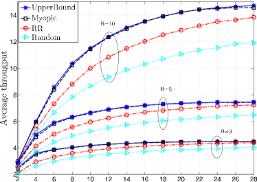
(a) $N/K$

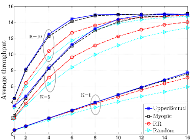
(b) Battery capacity ($B$)

Figure 2: (a) Average throughput vs. number of nodes, $N$, with $K=5$ channels, and battery capacity $B=3,5,10$, and (b) average throughput vs. battery capacity, $N=30$, and $K=1,5,10$.

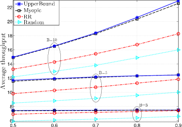
(a) $p_{11}$ ($p_{00}=0.5$)

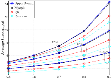
(b) $p_{11}$ ($p_{00}=0.9$)

Figure 3: Average throughput for different EH process transition probabilities, $N=30$, $K=5$, and $B=3,5,10$.

Figure 3 shows the average throughput for different EH process transition probabilities. We note that the amount of energy arriving to the system increases with $p_{11}$ and decreases with $p_{00}$. As expected, we observe in Figure 3 that the throughput increases with $p_{11}$, and the values in Figure 3(a) are notably higher than those in Figure 3(b). MP is a policy which maximises the immediate throughput at each TS, and does not take into account the future TSs. We observe in Figure 3(b) for $B=\{5,10\}$ and in Figure 3(a) for $B=10$ that, if the EH state has low correlation across TSs, that is, $p_{11}=\{0.5,0.6\}$, the throughput obtained by MP is similar to that of the upper bound. On the contrary, if it has high correlation across TSs, that is $p_{11}=\{0.8,0.9\}$, the throughput falls below the upper bound. This is due to the fact that when the state transitions have low correlation it is difficult to reliably predict the impact of the actions on the future rewards, and no transmission strategy can improve upon MP. Our numerical results indicate, that even in scenarios in which the MP cannot be shown to be theoretically optimal, it performs very close to the upper bound, obtained for an infinite horizon problem.

VIII Conclusions

We have studied a scheduling problem in a multi-access communication system with EH nodes, in which the harvested energy at each node is modeled as a Markov process. We have modeled the system as an RMAB problem, and shown the optimality of MP in two settings: i) when the nodes cannot harvest energy and transmit simultaneously and the EH process state is independent of the past states after a node is active; ii) when the nodes have no battery. The results of this paper suggest that although the optimal scheduling in large EH networks requires high computational complexity, in some cases there exist simple and practical scheduling policies that have almost optimal performance. This can have an impact on the design of scheduling policies for large low-power wireless sensor networks equipped with energy harvesting devices and limited storage.

Appendix A

We denote the probability that the battery of a node is not full if the node has been idle for the last $n$ TSs by $p_{nf}(n)$. It is easy to note that $p_{nf}(n)$ is a decreasing function of $n$. If the node has been idle for $n$ TSs, we denote the probability of the EH process being in state $0$ and $1$, by $p_{0}(n)\triangleq p_{10}+p_{0}(n-1)(p_{11}-p_{01})$ and $p_{1}(n)\triangleq 1-p_{0}(n)$, respectively. We set $p_{0}(0)=e_{0}$. Since $p_{11}\geq p_{01}$ and $e_{0}\leq\frac{p_{10}}{p_{01}+p_{10}}$, $p_{0}(n)$ monotonically increases to the steady state distribution ([22, Appendix B]).

We denote the belief state of a node that has been idle for $n$ TSs by $z_{n}$. If the node has been idle for $n+1$ TSs, the expected battery level is $z_{n+1}=\tau(z_{n})=z_{n}+\frac{p_{nf}(n)}{B}(p_{01}p_{0}(n)+p_{11}p_{1}(n))$, which is a monotonically increasing function. If $n\geq m$, then $z_{n}\geq z_{m}$ and $\tau(z_{n})\geq\tau(z_{m})$. By applying the definition of $p_{1}(n)$, we get $z_{n+1}=z_{n}+\frac{p_{nf}(n)}{B}(p_{11}-p_{0}(n)(p_{11}-p_{00}))$. If we assume that $n\geq m$, we have

$$\small]{rCL}\|\tau(z_{n})-\tau(z_{m})\| = z_{n}-z_{m}+\frac{p_{nf}(n)}{B}(p_{11}-p_{0}(n)(p_{11}-p_{01}))$$

$$-\frac{p_{nf}(m)}{B}(p_{11}\!-\!p_{0}(m)(p_{11}-p_{01}))$$

$$\leq z_{n}\!-\!z_{m}\!-\!\frac{p_{nf}(n)}{B}(p_{11}\!-\!p_{01})(p_{0}(n)\!-\!p_{0}(m))$$

$$\leq z_{n}-z_{m},$$

where the first inequality follows since $p_{nf}(n)\leq p_{nf}(m)$, and the second inequality follows since $p_{0}(n)$ is monotonically increasing and $p_{11}\geq p_{01}$.

Appendix B

The proof uses backward induction. We denote by $\mathcal{S}_{\mathbf{\accentset{\circ}{\text{$\Pi$}}}}^{K}$ and $\tilde{\mathcal{S}}_{\mathbf{\accentset{\circ}{\text{$\Pi$}}}}^{K}$ the nodes scheduled from $\mathbf{s}_{\mathbf{\accentset{\circ}{\text{$\Pi$}}}}$ and $\tilde{\mathbf{s}}_{\mathbf{\accentset{\circ}{\text{$\Pi$}}}}$, respectively. We first observe that (10) holds for $n=T$. This follows from the bounded regularity of $R(\cdot)$, noting that $u(T)=1$, and distinguishing four possible cases.

• Case $1$: $j\in\mathcal{S}_{\mathbf{\accentset{\circ}{\text{$\Pi$}}}}^{K}$ and $j\in\tilde{\mathcal{S}}_{\mathbf{\accentset{\circ}{\text{$\Pi$}}}}^{K}$, i.e., node $j$ is scheduled in both cases.

  $$\small]{rcl}W (\mathbf{s}_{\mathbf{\accentset{\circ}{\text{$\Pi$}}}})-W_{T}(\tilde{\mathbf{s}}_{\mathbf{\accentset{\circ}{\text{$\Pi$}}}})$$ _T

  $$= R(s_{\mathbf{\accentset{\circ}{\text{$\Pi$}}}(1)},\ldots,s_{j},\ldots,s_{\mathbf{\accentset{\circ}{\text{$\Pi$}}}(K)})-R(\tilde{s}_{\mathbf{\accentset{\circ}{\text{$\Pi$}}}(1)},\ldots,\tilde{s}_{j},\ldots,\tilde{s}_{\mathbf{\accentset{\circ}{\text{$\Pi$}}}(K)})$$

  $$= s_{j}R(s_{\mathbf{\accentset{\circ}{\text{$\Pi$}}}(1)},\ldots,1,\ldots,s_{\mathbf{\accentset{\circ}{\text{$\Pi$}}}(K)})+(1-s_{j})R(s_{\mathbf{\accentset{\circ}{\text{$\Pi$}}}(1)},\ldots,0,$$

  $$\ldots,s_{\mathbf{\accentset{\circ}{\text{$\Pi$}}}(K)})-\tilde{s}_{j}R(\tilde{s}_{\mathbf{\accentset{\circ}{\text{$\Pi$}}}(1)},\ldots,1,\ldots,\tilde{s}_{\mathbf{\accentset{\circ}{\text{$\Pi$}}}(K)})$$

  $$-(1-\tilde{s}_{j})R(\tilde{s}_{\mathbf{\accentset{\circ}{\text{$\Pi$}}}(1)},\ldots,0,\ldots,\tilde{s}_{\mathbf{\accentset{\circ}{\text{$\Pi$}}}(K)})$$

  $$= (s_{j}-\tilde{s}_{j})\big{(}R(s_{\mathbf{\accentset{\circ}{\text{$\Pi$}}}(1)},\ldots,1,\ldots,s_{\mathbf{\accentset{\circ}{\text{$\Pi$}}}(K)})$$

  $$-R(s_{\mathbf{\accentset{\circ}{\text{$\Pi$}}}(1)},\ldots,0,\ldots,s_{\mathbf{\accentset{\circ}{\text{$\Pi$}}}(K)})\big{)}$$

  $$\leq (s_{j}-{\tilde{s}_{j}})\Delta_{u}u(T),$$

  where the second equality follows from the decomposability of $R(\cdot)$. Since $R(\cdot)$ is symmetric and the belief vectors are equal but for node $j$, we have $R(s_{\mathbf{\accentset{\circ}{\text{$\Pi$}}}(1)},\ldots,\tilde{s}_{j}=k,\ldots,s_{\mathbf{\accentset{\circ}{\text{$\Pi$}}}(K)})=R(\tilde{s}_{\mathbf{\accentset{\circ}{\text{$\Pi$}}}(1)},\ldots,\tilde{s}_{j}=k,\ldots,\tilde{s}_{\mathbf{\accentset{\circ}{\text{$\Pi$}}}(N)})$, which we use in the third equality. Finally, the inequality follows from the boundedness of $R(\cdot)$.

• Case $2$: $j\notin\mathcal{S}_{\mathbf{\accentset{\circ}{\text{$\Pi$}}}}^{K}$ and $j\notin\tilde{\mathcal{S}}_{\mathbf{\accentset{\circ}{\text{$\Pi$}}}}^{K}$, i.e., node $j$ is not scheduled in either case. The same nodes with the same beliefs are scheduled in both cases, hence, $\mathbf{s}_{\mathbf{\accentset{\circ}{\text{$\Pi$}}}}^{K}=\tilde{\mathbf{s}}_{\mathbf{\accentset{\circ}{\text{$\Pi$}}}}^{K}$, and $W_{T}(\mathbf{s}_{\mathbf{\accentset{\circ}{\text{$\Pi$}}}})-W_{T}(\tilde{\mathbf{s}}_{\mathbf{\accentset{\circ}{\text{$\Pi$}}}})=0$.

• Case $3$: $j\in\mathcal{S}_{\mathbf{\accentset{\circ}{\text{$\Pi$}}}}^{K}$ and $j\notin\tilde{\mathcal{S}}_{\mathbf{\accentset{\circ}{\text{$\Pi$}}}}^{K}$. In this case there exists a node $m\in\tilde{\mathcal{S}}_{\mathbf{\accentset{\circ}{\text{$\Pi$}}}}^{K}$ such that $s_{j}\geq s_{m}\geq\tilde{s}_{j}$, and $m\notin\mathcal{S}_{\mathbf{\accentset{\circ}{\text{$\Pi$}}}}^{K}$

  $$\small]{lll}W (\mathbf{s}_{\mathbf{\accentset{\circ}{\text{$\Pi$}}}})-W_{T}(\tilde{\mathbf{s}}_{\mathbf{\accentset{\circ}{\text{$\Pi$}}}})$$ _T

  $$= (s_{j}-s_{m})\big{(}R(s_{\mathbf{\accentset{\circ}{\text{$\Pi$}}}(1)},\ldots,1,\ldots,s_{\mathbf{\accentset{\circ}{\text{$\Pi$}}}(K)})$$

  $$-R(s_{\mathbf{\accentset{\circ}{\text{$\Pi$}}}(1)},\ldots,0,\ldots,s_{\mathbf{\accentset{\circ}{\text{$\Pi$}}}(K)})\big{)}$$

  $$\leq (s_{j}-{\tilde{s}_{j}})\big{(}R(s_{\mathbf{\accentset{\circ}{\text{$\Pi$}}}(1)},\ldots,1,\ldots,s_{\mathbf{\accentset{\circ}{\text{$\Pi$}}}(K)})$$

  $$-R(s_{\mathbf{\accentset{\circ}{\text{$\Pi$}}}(1)},\ldots,0,\ldots,s_{\mathbf{\accentset{\circ}{\text{$\Pi$}}}(K)})\big{)}$$

  $$\leq (s_{j}-{\tilde{s}_{j}})\Delta_{u}u(T),$$

  where the first equality follows similar to Case $1$, the second equality from the fact that $s_{m}\geq\tilde{s}_{j}$, and the last inequality from the boundedness of $R(\cdot)$. Note that node $m$ is the node with the highest belief state that is not scheduled in $W_{T}(\mathbf{s}_{\mathbf{\accentset{\circ}{\text{$\Pi$}}}})$, and the node with the lowest belief state scheduled in $W_{T}(\tilde{\mathbf{s}}_{\mathbf{\accentset{\circ}{\text{$\Pi$}}}})$.

• Case $4$: $j\notin\mathcal{S}_{\mathbf{\accentset{\circ}{\text{$\Pi$}}}}^{K}$ and $j\in\tilde{\mathcal{S}}_{\mathbf{\accentset{\circ}{\text{$\Pi$}}}}^{K}$. This case is not possible since the vectors $\mathbf{s}_{\mathbf{\accentset{\circ}{\text{$\Pi$}}}}$ and $\tilde{\mathbf{s}}_{\mathbf{\accentset{\circ}{\text{$\Pi$}}}}$ are ordered and $s_{j}\geq{\tilde{s}_{j}}$, hence, if ${\tilde{s}_{j}}$ is scheduled then $s_{j}$ must be scheduled too.

Now, we assume that (10) holds from TS $n+1$ up to $T$, and show that it holds for TS $n$ as well. We distinguish three cases:

• Case $1$: $j\in\mathcal{S}_{\mathbf{\accentset{\circ}{\text{$\Pi$}}}}^{K}$ and $j\in\tilde{\mathcal{S}}_{\mathbf{\accentset{\circ}{\text{$\Pi$}}}}^{K}$ in (18), i.e., node $j$ is scheduled in both cases. The first and second summations in the first line of (18a) correspond to the cases in which node $j\in\mathcal{S}_{\mathbf{\accentset{\circ}{\text{$\Pi$}}}}^{K}$ is idle and active, respectively, in TS $n$. Similarly, first and second summations in the second line of (18a) correspond to the cases in which node $j\in\tilde{\mathcal{S}}_{\mathbf{\accentset{\circ}{\text{$\Pi$}}}}^{K}$ is idle and active, respectively, in TS $n$. Note that the belief state vector $\tilde{\mathbf{s}}_{\overline{\mathcal{E}\cup j}}$ includes the belief states of all the nodes in $\tilde{\mathbf{s}}_{\mathbf{\accentset{\circ}{\text{$\Pi$}}}}$, but those in $\mathcal{E}$ and $\tilde{s}_{j}$, hence, it is equivalent to the belief state vector $\mathbf{s}_{\overline{\mathcal{E}\cup{j}}}$. We use this fact to get (18b). Note that the belief state vectors in (18b) differ only in the belief states of node $j$, namely, $\tau(s_{j})$ and $\tau(\tilde{s}_{j})$ are the beliefs of node $j$ in vectors $[\mathrm{T}(\mathbf{s}_{\overline{\mathcal{E}}}),\mathbf{0}(|\mathcal{E}|)]$ and $[\mathrm{T}(\tilde{\mathbf{s}}_{\overline{\mathcal{E}}}),\mathbf{0}(|\mathcal{E}|)]$, respectively; and hence, we use the induction hypothesis in the summation of (18b) to obtain (18c). The summation in (18c) is over all possible operative/inoperative combinations of the nodes in $\mathcal{S}_{\mathbf{\accentset{\circ}{\text{$\Pi$}}}}^{K}\backslash\{j\}$, and it is equal to one. This fact together with the boundedness and the decomposability of $R(\cdot)$ are used in (18c) to get (18d). The contracting property of $\tau(\cdot)$, and the definition of $u(n)$ are used in (18e) and (18f), respectively.

  $$\normalsize]{rCL} W_{n} (\mathbf{s}_{\mathbf{\accentset{\circ}{\text{$\Pi$}}}})-W_{n}(\tilde{\mathbf{s}}_{\mathbf{\accentset{\circ}{\text{$\Pi$}}}})$$ (18a)

  $$= R(\mathbf{s}^{K}_{\mathbf{\accentset{\circ}{\text{$\Pi$}}}})+(1\!-\!p)\beta\displaystyle\!\!\!\!\!\!\!\!\!\sum_{\mathcal{E}\subseteq\mathcal{S}_{\mathbf{\accentset{\circ}{\text{$\Pi$}}}}^{K}\backslash\{j\}}\!\!\!\!\!\!\!\!q(|\mathcal{E}|,\!K\!\!-\!\!1)W_{n+1}([T(\mathbf{s}_{\overline{\mathcal{E}}}),\mathbf{0}(|\mathcal{E}|)])+p\beta\displaystyle\!\!\!\!\!\!\!\!\!\sum_{\mathcal{E}\subseteq\mathcal{S}_{\mathbf{\accentset{\circ}{\text{$\Pi$}}}}^{K}\backslash\{j\}}\!\!\!\!\!\!\!\!\!q(|\mathcal{E}|,\!K\!\!-\!\!1)W_{n+1}([T(\mathbf{s}_{\overline{\mathcal{E}\cup j}}),\mathbf{0}(|\mathcal{E}|\!\!+\!\!1)])$$

  $$- R(\tilde{\mathbf{s}}^{K}_{\mathbf{\accentset{\circ}{\text{$\Pi$}}}})\!-\!(1\!-\!p)\beta\displaystyle\!\!\!\!\!\!\!\!\!\sum_{\mathcal{E}\subseteq\tilde{\mathcal{S}}_{\mathbf{\accentset{\circ}{\text{$\Pi$}}}}^{K}\backslash\{j\}}\!\!\!\!\!\!\!\!\!q(|\mathcal{E}|,\!K\!\!-\!\!1)W_{n+1}([T(\tilde{\mathbf{s}}_{\overline{\mathcal{E}}}),\mathbf{0}(|\mathcal{E}|)])\!-p\beta\displaystyle\!\!\!\!\!\!\!\!\!\sum_{\mathcal{E}\subseteq\tilde{\mathcal{S}}_{\mathbf{\accentset{\circ}{\text{$\Pi$}}}}^{K}\backslash\{j\}}\!\!\!\!\!\!\!\!\!q(|\mathcal{E}|,\!K\!\!-\!\!1)W_{n+1}([T(\tilde{\mathbf{s}}_{\overline{\mathcal{E}\cup{j}}}),\mathbf{0}(|\mathcal{E}|\!\!+\!\!1)])$$

  $$= R(\mathbf{s}^{K}_{\mathbf{\accentset{\circ}{\text{$\Pi$}}}})-R(\tilde{\mathbf{s}}^{K}_{\mathbf{\accentset{\circ}{\text{$\Pi$}}}})+(1\!-\!p)\beta\displaystyle\!\!\!\!\!\!\!\!\!\sum_{\mathcal{E}\subseteq\mathcal{S}_{\mathbf{\accentset{\circ}{\text{$\Pi$}}}}^{K}\backslash\{j\}}\!\!\!\!\!\!\!\!\!q(|\mathcal{E}|,\!K\!\!-\!\!1)\Big{(}W_{n+1}([\mathrm{T}(\mathbf{s}_{\overline{\mathcal{E}}}),\mathbf{0}(|\mathcal{E}|)])-W_{n+1}([\mathrm{T}(\tilde{\mathbf{s}}_{\overline{\mathcal{E}}}),\mathbf{0}(|\mathcal{E}|)])\Big{)}$$ (18b)

  $$\leq R(\mathbf{s}^{K}_{\mathbf{\accentset{\circ}{\text{$\Pi$}}}})-R(\tilde{\mathbf{s}}^{K}_{\mathbf{\accentset{\circ}{\text{$\Pi$}}}})+(1\!-\!p)\beta\displaystyle\!\!\!\!\!\!\sum_{\mathcal{E}\subseteq\mathcal{S}_{\mathbf{\accentset{\circ}{\text{$\Pi$}}}}^{K}\backslash\{j\}}\!\!\!\!\!\!q(|\mathcal{E}|,\!K\!\!-\!\!1)\Big{(}\Delta_{u}(\tau(s_{j})-\tau(\tilde{s}_{j}))u(n+1)\Big{)}$$ (18c)

  $$\leq \Delta_{u}(s_{j}-\tilde{s}_{j})+(1\!-\!p)\beta\Delta_{u}(\tau(s_{j})-\tau(\tilde{s}_{j}))u(n+1)$$ (18d)

  $$\leq \Delta_{u}(s_{j}-\tilde{s}_{j})+(1\!-\!p)\beta\Delta_{u}(s_{j}-\tilde{s}_{j})u(n+1)$$ (18e)

  $$\leq \Delta_{u}(s_{j}-\tilde{s}_{j})\Big{(}1+\beta(1\!-\!p)\displaystyle\!\!\!\!\sum_{i=0}^{T-n-1}(\beta(1\!-\!p))^{i}\Big{)}$$ (18f)

  $$= \Delta_{u}(s_{j}-\tilde{s}_{j})u(n),$$ (18g)

  
  

• Case $2$:$j\notin\mathcal{S}_{\mathbf{\accentset{\circ}{\text{$\Pi$}}}}^{K}$ and $j\notin\tilde{\mathcal{S}}_{\mathbf{\accentset{\circ}{\text{$\Pi$}}}}^{K}$, i.e., the same nodes are scheduled from $\mathbf{s}_{\mathbf{\accentset{\circ}{\text{$\Pi$}}}}$ and $\tilde{\mathbf{s}}_{\mathbf{\accentset{\circ}{\text{$\Pi$}}}}$, and node $j$ is not scheduled in either case. Then

  $$\normalsize]{rCL}W_{n}(\mathbf{s}_{\mathbf{\accentset{\circ}{\text{$\Pi$}}}}) - W_{n}(\tilde{\mathbf{s}}_{\mathbf{\accentset{\circ}{\text{$\Pi$}}}})$$ (19a)

  $$= \beta\!\!\!\displaystyle\sum_{\mathcal{E}\subseteq\mathcal{S}_{\mathbf{\accentset{\circ}{\text{$\Pi$}}}}^{K}}\!\!\!q(|\mathcal{E}|,K)\Big{(}W_{n+1}([\mathrm{T}(\mathbf{s}_{\overline{\mathcal{E}}}),\mathbf{0}(|\mathcal{E}|)])$$

  $$-W_{n+1}([\mathrm{T}(\tilde{\mathbf{s}}_{\overline{\mathcal{E}}})\mathbf{0}(|\mathcal{E}|)])\Big{)}$$

  $$\leq \Delta_{u}(s_{j}-\tilde{s}_{j})\beta u(n+1)$$ (19b)

  $$\leq \Delta_{u}(s_{j}-\tilde{s}_{j})\beta\!\!\!\displaystyle\sum_{i=0}^{T-n-1}(\beta(1-p))^{i}$$ (19c)

  $$\leq \Delta_{u}(s_{j}-\tilde{s}_{j})u(n),$$ (19d)

  where (19a) follows since the value of the expected immediate rewards in TS $n$ are the same. The belief state vectors at TS $n+1$ are equal but for the belief state of node $j$, that is, $\tau(s_{j})$ and $\tau(\tilde{s}_{j})$ are the beliefs of node $j$ in $\mathrm{T}(\mathbf{s}_{\overline{\mathcal{E}}})$ and $\mathrm{T}(\tilde{\mathbf{s}}_{\overline{\mathcal{E}}})$, respectively. In (19a), similarly to (18c), (18d), and (18e), we apply the induction hypothesis, the contracting map property, and the fact that the summation is equal to one, to obtain (19b). We use $\beta\leq 1$ and the definition of $u(n)$ to obtain (19c) and (19d), respectively.

• Case $3$: $j\in\mathcal{S}_{\mathbf{\accentset{\circ}{\text{$\Pi$}}}}^{K}$ and $j\notin\tilde{\mathcal{S}}_{\mathbf{\accentset{\circ}{\text{$\Pi$}}}}^{K}$ in (20), i.e., there exists $m\in\tilde{\mathcal{S}}_{\mathbf{\accentset{\circ}{\text{$\Pi$}}}}^{K}$ such that $s_{j}\geq s_{m}=\tilde{s}_{m}\geq\tilde{s}_{j}$ and that $m\notin\mathcal{S}_{\mathbf{\accentset{\circ}{\text{$\Pi$}}}}^{K}$. Hence, $\mathcal{S}_{\mathbf{\accentset{\circ}{\text{$\Pi$}}}}^{K}$ and $\tilde{\mathcal{S}}_{\mathbf{\accentset{\circ}{\text{$\Pi$}}}}^{K}$ differ only in one element. To obtain (20d) we use the symmetry property of the pseudo value function and the fact that the belief vectors are equal but for node $j$; in (20d) we add and subtract a pseudo value function, which has two nodes with the same belief state $s_{m}$, and one is scheduled while the other is not. We can group the pseudo value functions, and apply the results of Case $1$ and Case $2$ above. In particular, for the pseudo value functions in the first line of (20d), the belief vectors are equal but for $s_{j}$ and $s_{m}$, moreover $j\in\mathcal{S}_{\mathbf{\accentset{\circ}{\text{$\Pi$}}}}^{K}$ and $m\in\tilde{\mathcal{S}}_{\mathbf{\accentset{\circ}{\text{$\Pi$}}}}^{K}$, and $s_{j}\geq s_{m}$, so we can apply the results of Case $1$. Similarly, for the two pseudo value functions in the second line of (20d) we can use the results of Case $2$.

  $$\normalsize]{rcl} W_{n} (s_{\mathbf{\accentset{\circ}{\text{$\Pi$}}}(1)},\dots,s_{j},\ldots,s_{\mathbf{\accentset{\circ}{\text{$\Pi$}}}(K)},s_{m},\ldots,s_{\mathbf{\accentset{\circ}{\text{$\Pi$}}}(N)})-W_{n}(\tilde{s}_{\mathbf{\accentset{\circ}{\text{$\Pi$}}}(1)},\dots,\tilde{s}_{m},\tilde{s}_{\mathbf{\accentset{\circ}{\text{$\Pi$}}}(K+1)},\dots,\tilde{s}_{j},\ldots,\tilde{s}_{\mathbf{\accentset{\circ}{\text{$\Pi$}}}(N)})$$ (20d)

  $$=W_{n}(s_{\mathbf{\accentset{\circ}{\text{$\Pi$}}}(1)},\dots,\!s_{j},\ldots,s_{\mathbf{\accentset{\circ}{\text{$\Pi$}}}(K)},\dots,s_{m},\ldots,s_{\mathbf{\accentset{\circ}{\text{$\Pi$}}}(N)})\!-\!\!W_{n}(s_{\mathbf{\accentset{\circ}{\text{$\Pi$}}}(1)},\dots,\!s_{m},\ldots,s_{\mathbf{\accentset{\circ}{\text{$\Pi$}}}(K)},\dots,\tilde{s}_{j},\ldots,s_{\mathbf{\accentset{\circ}{\text{$\Pi$}}}(N)})$$

  $$=W_{n}(s_{\mathbf{\accentset{\circ}{\text{$\Pi$}}}(1)},\dots,\!s_{j},\ldots,s_{\mathbf{\accentset{\circ}{\text{$\Pi$}}}(K)},\dots,\!s_{m},\ldots,s_{\mathbf{\accentset{\circ}{\text{$\Pi$}}}(N)})\!-\!\!W_{n}(s_{\mathbf{\accentset{\circ}{\text{$\Pi$}}}(1)},\dots,\!s_{m},\ldots,s_{\mathbf{\accentset{\circ}{\text{$\Pi$}}}(K)},\dots,\!s_{m},\ldots,s_{\mathbf{\accentset{\circ}{\text{$\Pi$}}}(N)})$$

  $$+W_{n}(s_{\mathbf{\accentset{\circ}{\text{$\Pi$}}}(1)},\dots,\!s_{m},\ldots,s_{\mathbf{\accentset{\circ}{\text{$\Pi$}}}(K)},\dots,\!s_{m},\ldots,s_{\mathbf{\accentset{\circ}{\text{$\Pi$}}}(N)})\!-\!\!W_{n}(s_{\mathbf{\accentset{\circ}{\text{$\Pi$}}}(1)},\dots,\!s_{m},\ldots,s_{\mathbf{\accentset{\circ}{\text{$\Pi$}}}(K)},\dots,\!\tilde{s}_{j},\ldots,s_{\mathbf{\accentset{\circ}{\text{$\Pi$}}}(N)})$$

  $$\leq\Delta_{u}(s_{j}-s_{m})u(n)+\Delta_{u}(s_{m}-\tilde{s}_{j})u(n)$$

  $$=\Delta_{u}(s_{j}-\tilde{s}_{j})u(n).$$

  
  

$$\normalsize]{rCL} W_{n} (\mathbf{s})-W_{n}(\mathbf{s}_{\Pi})$$ (21a)

$$= R(\mathbf{s}^{K})-R(\mathbf{s}^{K}_{\Pi})+\beta\displaystyle\!\!\!\!\!\sum_{\mathcal{E}\subseteq\mathcal{S}\backslash\{j\}}\!\!\!\!q(|\mathcal{E}|,K\!-\!1)\Big{(}pW_{n+1}\big{(}[\mathrm{T}(\mathbf{s}_{\overline{\mathcal{E}\cup j}}),\mathbf{0}(|\mathcal{E}|\!+\!1)]\big{)}+(1-p)W_{n+1}\big{(}[\mathrm{T}(\mathbf{s}_{\overline{\mathcal{E}}}),\mathbf{0}(|\mathcal{E}|)]\big{)}$$

$$\qquad\qquad\qquad\qquad\qquad\qquad\qquad-pW_{n+1}\big{(}[\mathrm{T}(\mathbf{s}_{\overline{\mathcal{E}\cup i}}),\mathbf{0}(|\mathcal{E}|\!+\!1)]\big{)}-(1-p)W_{n+1}\big{(}[\mathrm{T}(\mathbf{s}_{\overline{\mathcal{E}}}),\mathbf{0}(|\mathcal{E}|)]\big{)}\Big{)}$$

$$= R(\mathbf{s}^{K})-R(\mathbf{s}^{K}_{\Pi})-p\beta\displaystyle\!\!\!\!\!\sum_{\mathcal{E}\subseteq\mathcal{S}\backslash\{j\}}\!\!\!\!\!\!q(|\mathcal{E}|,K\!-\!1)\Big{(}W_{n+1}\big{(}[\mathrm{T}(\mathbf{s}_{\overline{\mathcal{E}\cup i}}),\mathbf{0}(|\mathcal{E}|\!+\!1)]\big{)}\!-\!W_{n+1}\big{(}[\mathrm{T}(\mathbf{s}_{\overline{\mathcal{E}\cup j}}),\mathbf{0}(|\mathcal{E}|\!+\!1)]\big{)}\Big{)}$$ (21b)

$$\geq \Delta_{l}(s_{j}-s_{i})-p\beta\displaystyle\!\!\!\!\!\sum_{\mathcal{E}\subseteq\mathcal{S}\backslash\{j\}}\!\!\!\!q(|\mathcal{E}|,K\!-\!1)\Big{(}W_{n+1}\big{(}[\mathrm{T}(\mathbf{s}_{\overline{\mathcal{E}\cup i}}),\mathbf{0}(|\mathcal{E}|\!+\!1)]\big{)}-W_{n+1}\big{(}[\mathrm{T}(\mathbf{s}_{\overline{\mathcal{E}\cup j}}),\mathbf{0}(|\mathcal{E}|\!+\!1)]\big{)}\Big{)}$$ (21c)

$$\geq \Delta_{l}(s_{j}-s_{i})-p\beta\displaystyle\!\!\!\!\!\sum_{\mathcal{E}\subseteq\mathcal{S}\backslash\{j\}}\!\!\!\!\Big{(}q(|\mathcal{E}|,K\!-\!1)\Delta_{u}(\tau(s_{j})-\tau(s_{i}))u(n+1)\Big{)}$$ (21d)

$$\geq \Delta_{l}(s_{j}-s_{i})-p\beta\Delta_{u}(s_{j}-s_{i})u(n+1)$$ (21e)

$$\geq \Delta_{l}(s_{j}-s_{i})-p\beta\Delta_{u}(s_{j}-s_{i})u(0)$$ (21f)

$$= (s_{j}-s_{i})\left(\Delta_{l}-p\beta\frac{1-\beta(1-p)^{T+1}}{1-\beta(1-p)}\Delta_{u}\right)\geq 0$$ (21g)

Appendix C

We note that set $\mathcal{S}=\{1,\ldots,K\}$ is the set of $K$ nodes scheduled from $\mathbf{s}$, and that the set $\mathcal{S}_{\Pi}^{K}$ is the set of nodes scheduled from $\mathbf{s}_{\Pi}$, that is, the first $K$ nodes as ordered according to permutation $\Pi$. We only need to study the cases in which $\mathcal{S}$ and $\mathcal{S}_{\Pi}^{K}$ are different, since the claim holds for the others due to the symmetric property of the pseudo value function, (8). We study the case $j\in\mathcal{S}$, $i\in\mathcal{S}_{\Pi}^{K}$, $i\notin\mathcal{S}$, and $j\notin\mathcal{S}_{\Pi}^{K}$ in (21). The summation in (21a) is over all operative/inoperative combinations of the nodes in $\mathcal{S}\backslash\{j\}$. We denote the belief state of all nodes but those in $\mathcal{E}$ and $s_{j}$ by $\mathbf{s}_{\overline{\mathcal{E}\cup j}}$. The belief state of node $i$ in TS $n+1$, $\tau(s_{i})$, is in vector $\mathrm{T}(\mathbf{s}_{\overline{\mathcal{E}\cup j}})$. Similarly, the belief state of node $j$ in TS $n+1$, $\tau(s_{j})$, is in vector $\mathrm{T}(\mathbf{s}_{\overline{\mathcal{E}\cup i}})$. The second pseudo value functions in the first and second lines in (21a) cancel out, and (21b) is obtained. We have applied the decomposability and boundedness of $R(\cdot)$ to obtain (21c). Belief vectors $\mathrm{T}(\mathbf{s}_{\overline{\mathcal{E}\cup j}})$ and $\mathrm{T}(\mathbf{s}_{\overline{\mathcal{E}\cup i}})$ in (21c) are ordered and only differ in one element, $\tau(s_{i})$ and $\tau(s_{j})$, respectively, where $\tau(s_{i})\leq\tau(s_{j})$, and hence, we use Lemma 2 to get (21d); (21e) follows since $\tau(\cdot)$ is a monotonically increasing contracting map, (21f) since $u(n)$ is decreasing in $n$; finally (21g) follows since $u(0)$ is the sum of a geometric series.

Appendix D

We again use backward induction. Lemma 4 holds trivially for $n=T$. Note that in (15a) the set of nodes scheduled in the pseudo value functions $W_{n}(\mathbf{s}_{\mathbf{\widehat{\text{$\Pi$}}}})$ and $W_{n}(\mathbf{s})$ are $\{1,\ldots,K-1,N\}$ and $\{1,\ldots,K\}$, respectively. That is, node $K$ is scheduled in $W_{n}(\mathbf{s})$, but not in $W_{n}(\mathbf{s}_{\mathbf{\widehat{\text{$\Pi$}}}})$; and node $N$ is scheduled in $W_{n}(\mathbf{s}_{\mathbf{\widehat{\text{$\Pi$}}}})$, but not in $W_{n}(\mathbf{s})$. To prove that (15a) holds at TS $n$ we use a sample path argument similarly to [17], and assume that the realizations of the EH processes of nodes $K$ and $N$ are either $0$ or $1$. There are four different cases, but here we only consider one, since the others follow similarly.

We consider the case in which the EH processes have realizations $E^{s}_{K}(n)=1$ and $E^{s}_{N}(n)=0$. We denote by $\mathcal{K}=\{1,\ldots,K-1\}$ the set of nodes scheduled in both sides of (15a). If $\mathcal{E}$ is the set of active nodes, we denote the set of nodes in $\mathcal{K}$ that remain idle by $\mathcal{K}^{i}=\mathcal{K}\backslash\mathcal{E}$. We denote the nodes that are not scheduled in either side of (15a) by $\mathcal{K}^{s}=\overline{\mathcal{K}\cup\{K,N\}}$. We denote the set $\{0,1\}^{|\mathcal{E}|}$ by $\mathcal{B}^{|\mathcal{E}|}$. From the left hand side of (15a) we obtain (22), where in (22d) we have applied the induction hypothesis of (15a), the symmetry of the pseudo value function, the inequality $p_{11}\geq p_{00}$, and the definition of $R(\cdot)$. This concludes the proof of (15a).

$$\normalsize]{rCL}1 + W_{n}(s_{N},s_{1},\ldots,s_{N-1})$$ (22d)

$$= 1+R(\mathbf{s}_{\mathbf{\widehat{\text{$\Pi$}}}}^{K})+\beta\!\!\displaystyle\sum_{\mathcal{E}\subseteq\mathcal{K}}\!\!\!\!\!\!\!\displaystyle\sum_{\leavevmode\nobreak\ \leavevmode\nobreak\ \leavevmode\nobreak\ \leavevmode\nobreak\ l_{\mathcal{E}}\in\mathcal{B}^{|\mathcal{E}|}}\!\!\!\!\!\!h(l_{\mathcal{E}},K\!-\!1)\Big{[}pW_{n+1}\left(\mathbf{P}_{11}\left(\Sigma l_{\mathcal{E}}\right),\boldsymbol{\tau}(\mathbf{s}_{\mathcal{K}^{i}}),s_{K}=p_{11},\boldsymbol{\tau}(\mathbf{s}_{\mathcal{K}^{s}}),s_{N}=p_{01},\mathbf{P}_{01}\left(\overline{\Sigma}l_{\mathcal{E}}\right)\right)$$

$$\qquad\qquad\qquad\qquad+(1-p)W_{n+1}\left(\mathbf{P}_{11}\left(\Sigma l_{\mathcal{E}}\right),s_{N}=p_{01},\boldsymbol{\tau}(\mathbf{s}_{\mathcal{K}^{i}}),s_{K}=p_{11},\boldsymbol{\tau}(\mathbf{s}_{\mathcal{K}^{s}}),\mathbf{P}_{01}\left(\overline{\Sigma}l_{\mathcal{E}}\right)\right)\Big{]}$$

$$\geq p+R(\mathbf{s}_{\mathbf{\widehat{\text{$\Pi$}}}}^{K})+\beta\!\!\displaystyle\sum_{\mathcal{E}\subseteq\mathcal{K}}\!\!\!\!\!\!\!\displaystyle\sum_{\leavevmode\nobreak\ \leavevmode\nobreak\ \leavevmode\nobreak\ \leavevmode\nobreak\ l_{\mathcal{E}}\in\mathcal{B}^{|\mathcal{E}|}}\!\!\!\!\!\!h(l_{\mathcal{E}},K\!-\!1)\Big{[}pW_{n+1}\left(\mathbf{P}_{11}\left(\Sigma l_{\mathcal{E}}\right),\boldsymbol{\tau}(\mathbf{s}_{\mathcal{K}^{i}}),s_{K}=p_{11},\boldsymbol{\tau}(\mathbf{s}_{\mathcal{K}^{s}}),s_{N}=p_{01},\mathbf{P}_{01}\left(\overline{\Sigma}l_{\mathcal{E}}\right)\right)$$

$$\qquad\qquad\qquad\qquad+(1-p)\Big{(}1+W_{n+1}\left(\mathbf{P}_{11}\left(\Sigma l_{\mathcal{E}}\right),s_{N}=p_{01},\boldsymbol{\tau}(\mathbf{s}_{\mathcal{K}^{i}}),s_{K}=p_{11},\boldsymbol{\tau}(\mathbf{s}_{\mathcal{K}^{s}}),\mathbf{P}_{01}\left(\overline{\Sigma}l_{\mathcal{E}}\right)\Big{)}\right)\Big{]}$$

$$\geq p+R(\mathbf{s}_{\mathbf{\widehat{\text{$\Pi$}}}}^{K})+\beta\!\!\displaystyle\sum_{\mathcal{E}\subseteq\mathcal{K}}\!\!\!\!\!\!\!\displaystyle\sum_{\leavevmode\nobreak\ \leavevmode\nobreak\ \leavevmode\nobreak\ \leavevmode\nobreak\ l_{\mathcal{E}}\in\mathcal{B}^{|\mathcal{E}|}}\!\!\!\!\!\!h(l_{\mathcal{E}},K\!-\!1)\Big{[}pW_{n+1}\left(\mathbf{P}_{11}\left(\Sigma l_{\mathcal{E}}\right),\boldsymbol{\tau}(\mathbf{s}_{\mathcal{K}^{i}}),s_{K}=p_{11},\boldsymbol{\tau}(\mathbf{s}_{\mathcal{K}^{s}}),s_{N}=p_{01},\mathbf{P}_{01}\left(\overline{\Sigma}l_{\mathcal{E}}\right)\right)$$

$$\qquad\qquad\qquad\qquad+(1-p)W_{n+1}\left(\mathbf{P}_{11}\left(\Sigma l_{\mathcal{E}}\right),\boldsymbol{\tau}(\mathbf{s}_{\mathcal{K}^{i}}),s_{K}=p_{11},\boldsymbol{\tau}(\mathbf{s}_{\mathcal{K}^{s}}),\mathbf{P}_{01}\left(\overline{\Sigma}l_{\mathcal{E}}\right),s_{N}=p_{01}\right)\Big{]}$$

$$= R(\mathbf{s}^{K})+\beta\!\!\displaystyle\sum_{\mathcal{E}\subseteq\mathcal{K}}\!\!\!\!\!\!\!\displaystyle\sum_{\leavevmode\nobreak\ \leavevmode\nobreak\ \leavevmode\nobreak\ \leavevmode\nobreak\ l_{\mathcal{E}}\in\mathcal{B}^{|\mathcal{E}|}}\!\!\!\!\!\!h(l_{\mathcal{E}},K\!-\!1)\Big{[}pW_{n+1}\left(\mathbf{P}_{11}\left(\Sigma l_{\mathcal{E}}\right),s_{K}=p_{11},\boldsymbol{\tau}(\mathbf{s}_{\mathcal{K}^{i}}),\boldsymbol{\tau}(\mathbf{s}_{\mathcal{K}^{s}}),s_{N}=p_{01},\mathbf{P}_{01}\left(\overline{\Sigma}l_{\mathcal{E}}\right)\right)$$

$$\qquad\qquad\qquad\qquad+(1-p)W_{n+1}\left(\mathbf{P}_{11}\left(\Sigma l_{\mathcal{E}}\right),\boldsymbol{\tau}(\mathbf{s}_{\mathcal{K}^{i}}),s_{K}=p_{11},\boldsymbol{\tau}(\mathbf{s}_{\mathcal{K}^{s}}),s_{N}=p_{01},\mathbf{P}_{01}\left(\overline{\Sigma}l_{\mathcal{E}}\right)\right)\Big{]}$$

$$= W_{n}(\mathbf{s})$$ (22e)

$$\normalsize]{rCL}W_{n}(\tilde{\mathbf{s}}) = R(\tilde{\mathbf{s}}^{K})+\beta\!\!\displaystyle\sum_{\mathcal{E}\subseteq\mathcal{K}}\!\!\!\!\!\!\!\!\displaystyle\sum_{\leavevmode\nobreak\ \leavevmode\nobreak\ \leavevmode\nobreak\ \leavevmode\nobreak\ l_{\mathcal{E}}\in\mathcal{B}^{|\mathcal{E}|}}\!\!\!\!\!\!h(l_{\mathcal{E}},K\!-\!1)\Big{[}pW_{n+1}\left(\mathbf{P}_{11}\left(\Sigma l_{\mathcal{E}}\right),s_{j}=p_{11},\boldsymbol{\tau}(\mathbf{s}_{\mathcal{K}^{i}}),\boldsymbol{\tau}(\mathbf{s}_{\mathcal{K}^{s}\cup i}),\mathbf{P}_{01}\left(\overline{\Sigma}l_{\mathcal{E}}\right)\right)$$ (23c)

$$\qquad\qquad\qquad\qquad\qquad\qquad+(1-p)W_{n+1}\left(\mathbf{P}_{11}\left(\Sigma l_{\mathcal{E}}\right),\boldsymbol{\tau}(\mathbf{s}_{\mathcal{K}^{i}\cup j}),\boldsymbol{\tau}(\mathbf{s}_{\mathcal{K}^{s}\cup i}),\mathbf{P}_{01}\left(\overline{\Sigma}l_{\mathcal{E}}\right)\right)\Big{]}$$

$$\geq R(\tilde{\mathbf{s}}^{K})-p+\beta\!\!\displaystyle\sum_{\mathcal{E}\subseteq\mathcal{K}}\!\!\!\!\!\!\!\!\displaystyle\sum_{\leavevmode\nobreak\ \leavevmode\nobreak\ \leavevmode\nobreak\ \leavevmode\nobreak\ l_{\mathcal{E}}\in\mathcal{B}^{|\mathcal{E}|}}\!\!\!\!\!\!h(l_{\mathcal{E}},K\!-\!1)\Big{[}p\Big{(}1+W_{n+1}\left(\mathbf{P}_{11}\left(\Sigma l_{\mathcal{E}}\right),s_{i}=p_{01},\boldsymbol{\tau}(\mathbf{s}_{\mathcal{K}^{i}}),\boldsymbol{\tau}(\mathbf{s}_{\mathcal{K}^{s}\cup j}),\mathbf{P}_{01}\left(\overline{\Sigma}l_{\mathcal{E}}\right)\right)\Big{)}$$

$$\qquad\qquad\qquad\qquad\qquad\qquad+(1-p)W_{n+1}\left(\mathbf{P}_{11}\left(\Sigma l_{\mathcal{E}}\right),\boldsymbol{\tau}(\mathbf{s}_{\mathcal{K}^{i}\cup i}),\boldsymbol{\tau}(\mathbf{s}_{\mathcal{K}^{s}\cup j}),\mathbf{P}_{01}\left(\overline{\Sigma}l_{\mathcal{E}}\right)\right)\Big{]}$$

$$\geq R(\tilde{\mathbf{s}}^{K})-p+\beta\!\!\displaystyle\sum_{\mathcal{E}\subseteq\mathcal{K}}\!\!\!\!\!\!\!\!\displaystyle\sum_{\leavevmode\nobreak\ \leavevmode\nobreak\ \leavevmode\nobreak\ \leavevmode\nobreak\ l_{\mathcal{E}}\in\mathcal{B}^{|\mathcal{E}|}}\!\!\!\!\!\!h(l_{\mathcal{E}},K\!-\!1)\Big{[}pW_{n+1}\left(\mathbf{P}_{11}\left(\Sigma l_{\mathcal{E}}\right),\boldsymbol{\tau}(\mathbf{s}_{\mathcal{K}^{i}}),\boldsymbol{\tau}(\mathbf{s}_{\mathcal{K}^{s}\cup j}),\mathbf{P}_{01}\left(\overline{\Sigma}l_{\mathcal{E}}\right),s_{i}=p_{01}\right)$$

$$\qquad\qquad\qquad\qquad\qquad\qquad+(1-p)W_{n+1}\left(\mathbf{P}_{11}\left(\Sigma l_{\mathcal{E}}\right),\boldsymbol{\tau}(\mathbf{s}_{\mathcal{K}^{i}\cup i}),\boldsymbol{\tau}(\mathbf{s}_{\mathcal{K}^{s}\cup j}),\mathbf{P}_{01}\left(\overline{\Sigma}l_{\mathcal{E}}\right)\right)\Big{]}$$

$$= W_{n}(\tilde{\mathbf{s}}_{\Pi})$$ (23d)

Now we prove the second part of Lemma 4, (15b). There are three cases:

• Case $1$: $j,i\leq K$, i.e., nodes $j$ and $i$ are scheduled on both sides of (15b). The inequality holds since the pseudo value function is symmetric.

• Case $2$: $j\leq K$ and $i>K$ in (23), i.e., nodes $i$ and $j$ are scheduled on the left and right hand sides of (15b), respectively. To prove the inequality we use the linearity of the pseudo value function (14). Since $s_{j}\geq s_{i}$, using (14), we only need to prove that $W_{n}(s_{1},\ldots,1,\ldots,0,\ldots,s_{N})-W_{n}(s_{1},\ldots,0,\ldots,1,\ldots,s_{N})\geq 0$. We denote the scheduled nodes in both sides of (15b) by $\mathcal{K}=\{1,\ldots,K\}\backslash\{j\}$, the set of nodes in $\mathcal{K}$ that remain idle by $\mathcal{K}^{i}=\mathcal{K}\backslash\mathcal{E}$, and the nodes that are not scheduled in either side of (15b) by $\mathcal{K}^{s}=\overline{\mathcal{K}\cup\{j,i\}}$. We denote the belief vector $(s_{1},\ldots,s_{j}=1,\ldots,s_{i}=0,\ldots,s_{N})$ by $\tilde{\mathbf{s}}$, its $i,j$-swap by $\tilde{\mathbf{s}}_{\Pi}$, and define $\tilde{\mathbf{s}}^{K}\triangleq(\tilde{s}_{1},\ldots,\tilde{s}_{K})$. In (23) have used the induction hypothesis of (15b) and (15a) in (23c) and (23c), respectively, and the fact that $\beta\leq 1$.

• Case $3$: nodes $s_{j}$ and $s_{i}$ are not scheduled. Inequality holds in this case, by applying the definition of (13) and the induction hypothesis of (15b).

Pol Blasco received the B.Eng. degree from Technische Universität Darmstadt, Germany, and BarcelonaTech (formally UPC), Spain, in 2008 and 2009, respectively, the M. S. degree from BarcelonaTech, in 2011, and the Ph.D. degree in electrical engineering from Imperial College London, in 2014. He was research assistant at CTTC in Barcelona, Spain, from November 2009 until August 2013. He was a visiting scholar in the Centre for Wireless Communication in University of Oulu, Finland, during the last semester of 2011, and to Imperial College during the first half of 2013. In 2008 he pursued the B.Eng. thesis in European Space Operation Center in the OPS-GSS section, Darmstadt, Germany. He also has carried on research in neuroscience in IDIBAPS, Barcelona, Spain, and in the Technische Universität Darmstadt in collaboration with the Max-Planck-Institut, Frankfurt, Germany, in 2009 and 2008, respectively. His current research interest cover communication of energy harvesting devices, cognitive radio, machine learning, control theory, decision making, and neuroscience.

Deniz Gündüz (S’03-M’08-SM’13) received the M.S. and Ph.D. degrees in electrical engineering from NYU Polytechnic School of Engineering in 2004 and 2007, respectively. After his PhD he served as a postdoctoral research associate at Princeton University, and as a consulting assistant professor at Stanford University. Since September 2012 he is a Lecturer in the Electrical and Electronic Engineering Department of Imperial College London. Previously he was a research associate at CTTC in Barcelona, Spain. He also held a visiting researcher position at Princeton University from November 2009 until November 2011. Dr. Gunduz is an Associate Editor of the IEEE TRANSACTIONS ON COMMUNICATIONS. He is serving as a co-chair of the IEEE Information Theory Society Student Committee, and a co-director of the Imperial College Probability Center. He has served as the co-chair of the Network Theory Symposium at the 2013 and 2014 IEEE Global Conference on Signal and Information Processing (GlobalSIP), and he was a co-chair of the 2012 IEEE European School of Information Theory (ESIT). His research interests lie in the areas of communication theory and information theory with special emphasis on joint source-channel coding, multi-user networks, energy efficient communications and privacy.

References

• [1] D. Gunduz, K. Stamatiou, N. Michelusi, and M. Zorzi, “Designing intelligent energy harvesting communication systems,” IEEE Commun. Mag., vol. 52, no. 1, pp. 210–216, Jan. 2014.
• [2] J. Yang and S. Ulukus, “Optimal packet scheduling in an energy harvesting communication system,” IEEE Trans. Commun., vol. 60, no. 1, pp. 220–230, Jan. 2012.
• [3] B. Devillers and D. Gündüz, “A general framework for the optimization of energy harvesting communication systems,” J. of Commun. and Nerworks., Special Issue on Energy Harvesting in Wireless Networks, vol. 14, no. 2, pp. 130–139, Apr. 2012.
• [4] Z. Wang, A. Tajer, and X. Wang, “Communication of energy harvesting tags,” IEEE Trans. Commun., vol. 60, no. 4, pp. 1159–1166, Apr. 2012.
• [5] A. Aprem, C. Murthy, and N. Mehta, “Transmit power control policies for energy harvesting sensors with retransmissions,” IEEE J. of Selected Topics in Signal Processing, vol. 7, no. 5, pp. 895–906, Oct. 2013.
• [6] J. Lei, R. Yates, and L. Greenstein, “A generic model for optimizing single-hop transmission policy of replenishable sensors,” IEEE Trans. Wireless Commun., vol. 8, no. 4, pp. 547–551, Apr. 2009.
• [7] N. Michelusi and M. Zorzi, “Optimal random multiaccess in energy harvesting wireless sensor networks,” in IEEE Int’l Conference on Communications - E2Nets Workshop, Budapest, Hungary, Jun. 2013.
• [8] F. Iannello, O. Simeone, and U. Spagnolini, “Optimality of myopic scheduling and Whittle indexability for energy harvesting sensors,” in Conf. on Information Sciences and Systems (CISS), Princeton, NJ, Mar. 2012, pp. 1–6.
• [9] P. Blasco, D. Gündüz, and M. Dohler, “Low-complexity scheduling policies for energy harvesting communication networks,” in IEEE International Symposium on Information Theory (ISIT), Istanbul, Turkey, Jul. 2013.
• [10] O. M. Gul and E. Uysal-Biyikoglu, “A randomized scheduling algorithm for energy harvesting wireless sensor networks achieving nearly $100\%$ throughput,” in IEEE Wireless Communications and Networking Conference (WCNC), Istanbul, Turkey, Apr. 2014.
• [11] P. Blasco, D. Gündüz, and M. Dohler, “A learning theoretic approach to energy harvesting communication system optimization,” IEEE Trans. Wireless Commun., vol. 12, no. 4, pp. 1872–1882, Apr. 2013.
• [12] D. P. Bertsekas, Dynamic Programming and Optimal Control.   Athenea Scientific, 2005.
• [13] M. L. Littman, T. L. Dean, and L. P. Kaelbling, “On the complexity of solving Markov decision problems,” in Conference on Uncertainty in Artificial Intelligence (UAI), Montreal, QU, Aug. 1995, pp. 394–402.
• [14] P. Whittle, “Restless bandits: Activity allocation in a changing world,” Journal of Applied Probability, a celabration of Applied Probability, vol. 25, pp. 287–298, 1988.
• [15] C. H. Papadimitriou and J. Tsitsiklis, “The complexity of optimal queueing network control,” in Structure in Complexity Theory Conference, Amsterdam, The Netherlands, Jun. 1994, pp. 318–322.
• [16] S. H. A. Ahmad, M. Liu, T. Javidi, Q. Zhao, and B. Krishnamachari, “Optimality of myopic sensing in multichannel opportunistic access,” IEEE Trans. Inf. Theory, vol. 55, no. 9, pp. 4040–4050, Sep. 2009.
• [17] S. H. A. Ahmad and M. Liu, “Multi-channel opportunistic access: A case of restless bandits with multiple plays,” in Allerton conference on Communication, Control, and Computing, Monticello, IL, Sep. 2009, pp. 1361–1368.
• [18] P. Mansourifard, T. Javidi, and B. Krishnamachari, “Optimality of myopic policy for a class of monotone affine restless multi-armed bandits,” in IEEE Conference on Decision and Control (CDC), Grand Wailea Maui, HI, USA, Dec. 2012, pp. 877–882.
• [19] K. Wang and L. Chen, “On optimality of myopic policy for restless multi-armed bandit problem: An axiomatic approach,” IEEE Trans. Signal Process., vol. 60, no. 1, pp. 300–309, Jan 2012.
• [20] K. Liu, Q. Zhao, and B. Krishnamachari, “Dynamic multichannel access with imperfect channel state detection,” IEEE Trans. Signal Process., vol. 58, no. 5, pp. 2795–2808, May 2010.
• [21] D. Bertsimas and J. Niño-Mora, “Restless bandits, linear programming relaxations, and primal-dual index heuristic,” Operational Research, vol. 48, no. 1, pp. 80–90, Jan.-Feb. 2000.
• [22] Q. Zhao, Krishnamachari, and K. Liu, “On myopic sensing for multi-channel opportunistic access: Structure, optimality and performance,” IEEE Trans. Wireless Commun., vol. 7, no. 12, pp. 5431–5440, Dec. 2008.