Towards a splitter theorem for internally $4$-connected binary matroids VIII: small matroids

Abstract.

Our splitter theorem for internally $4$-connected binary matroids studies pairs of the form $(M,N)$, where $M$ and $N$ are internally $4$-connected binary matroids, $M$ has a proper $N$-minor, and if $M^{\prime}$ is an internally $4$-connected matroid such that $M$ has a proper $M^{\prime}$-minor and $M^{\prime}$ has an $N$-minor, then $|E(M)|-|E(M^{\prime})|>3$. The analysis in the splitter theorem requires the constraint that $|E(M)|\geq 16$. In this article, we complement that analysis by using an exhaustive computer search to find all such pairs for which $|E(M)|\leq 15$.

1. Introduction

A matroid is internally $4$-connected if it is $3$-connected and $\min\{|X|,|Y|\}=3$ for any $3$-separation, $(X,Y)$. For some time, we have been engaged in a project to develop a splitter theorem for internally $4$-connected binary matroids [2, 3, 4, 5, 6, 7, 8, 9]. This means that we are concerned with understanding what we refer to here as interesting pairs. If $N$ and $M$ are matroids, we write $N\preceq M$ to mean that $M$ has an $N$-minor, and $N\prec M$ to mean that $M$ has a proper $N$-minor. An interesting pair is a pair $(M,N)$, where $M$ and $N$ are internally $4$-connected binary matroids such that

• $|E(N)|\geq 6$;

• $N\prec M$;

• if $M^{\prime}$ is an internally $4$-connected matroid for which $N\preceq M^{\prime}\prec M$, then $|E(M)|-|E(M^{\prime})|>3$.

Note that the last condition means that $|E(M)|-|E(N)|>3$. We say that an interesting pair, $(M,N)$, is a fascinating pair if $M^{\prime}$ is isomorphic to $N$ whenever $M^{\prime}$ is an internally $4$-connected matroid satisfying $N\preceq M^{\prime}\prec M$. Thus an interesting pair is fascinating if there is no intermediate internally $4$-connected matroid in the minor order.

It has been known for some time (see, for example, [11]) that there are fascinating pairs with $|E(M)|-|E(N)|$ arbitrarily large; indeed, this is true even if we insist that $M$ and $N$ are graphic matroids, since we can produce a fascinating pair by setting $N$ to be the graphic matroid of a cubic planar ladder, and letting $M$ be the graphic matroid of a quartic planar ladder on the same number of vertices. However, our project has shown that only a small number of constructions are needed to build $M$ from $N$, whenever $(M,N)$ is a fascinating pair.

The analysis in our project requires $M$ to be a certain size, in particular, $|E(M)|\geq 16$. To complement this analysis, our results here contain a description of all interesting pairs for which $|E(M)|\leq 15$. Our first theorem will describe the fascinating pairs. Up to duality, there are exactly $31$. Before that, we introduce some important matroids and graphs.

For $n\geq 3$, we denote the cubic Möbius ladder on $2n$ vertices by $\mathit{CM}_{2n}$. This graph is obtained from an even cycle on $2n$ vertices by joining each vertex to the antipodal vertex (the vertex of distance $n$). Similarly, for $n\geq 2$, the quartic Möbius ladder on $2n+1$ vertices is denoted by $\mathit{QM}_{2n+1}$, and is obtained from an odd cycle with $2n+1$ vertices by joining each vertex to the two vertices of distance $n$. Note that $\mathit{QM}_{5}$ is isomorphic to $K_{5}$, and $\mathit{CM}_{6}$ is isomorphic to $K_{3,3}$.

The Möbius matroids have been discovered in several contexts [13, 14]. For each positive integer $n\geq 3$, let $\mathcal{W}_{n}$ be the wheel with $n+1$ vertices, and let $B$ be the set of spoke edges. Thus $B$ is a basis of the rank-$n$ binary matroid $M({\mathcal{W}}_{n})$. Let $M_{n}$ be the binary matroid obtained from $M({\mathcal{W}}_{n})$ by adding a single element, $\gamma$, so that the fundamental circuit $C(\gamma,B)$ is $B\cup\gamma$. Kingan and Lemos [13] denote $M_{n}$ by $F_{2n+1}$. Observe that $M_{3}$ is the Fano matroid, and $M_{4}\cong M^{*}(K_{3,3})$. When $n$ is odd, $M_{n}^{*}$ is the rank-$(n+1)$ triadic Möbius matroid, denoted by $\Upsilon_{n+1}$. Hence $\Upsilon_{4}\cong F_{7}^{*}$. Moreover, $\Upsilon_{6}$ is isomorphic to any single-element deletion of $T_{12}$, the rank-$6$ binary matroid introduced by Kingan [12]. We also observe that $\Upsilon_{n+1}\backslash\gamma\cong M^{*}(\mathit{QM}_{n})$.

For $n\geq 3$, we construct the graph $G_{n+2}^{+}$ by starting with an $n$-vertex cycle, $C$, containing adjacent vertices $x$ and $y$, and then adding two additional vertices, $u$ and $w$, and making both of them adjacent to every vertex in $C$. We join $u$ and $w$ with an edge $\gamma$. Note that the planar dual of $G_{n+2}^{+}\backslash\gamma$ is $\mathit{CM}_{2n}$. Let $\Delta_{n+1}$ be the binary matroid that is obtained from $M(G_{n+2}^{+})$ by deleting the element $xy$ and adding a new element so that it forms a circuit with the elements $wx$ and $uy$. This new element also forms a circuit with $ux$ and $wy$. We also define $\Delta_{3}$ to be $F_{7}$. Then $\Delta_{r}$ is the rank-$r$ triangular Möbius matroid. Observe that $\Delta_{n+1}\backslash\gamma\cong M^{*}(\mathit{CM}_{2n})$. Kingan and Lemos [13] use $B_{3n+1}$ to denote $G_{n+2}^{+}$, and $S_{3n+1}$ to denote $\Delta_{n+1}$.

Now we give our description of fascinating pairs. Any graphs or matroids which we have not yet defined will be introduced in Section 3. For now, we note that $Q_{3}$ is the cube graph; $O$ is the octahedron graph; $H_{1}$, $H_{2}$, and $H_{3}$ are graphs with $13$ edges, and, respectively, $6$, $7$, and $8$ vertices; $Q_{3}^{\times}$ and $Y_{9}$ have $14$ edges and, respectively, $8$ and $9$ vertices; $A_{1}$, $A_{2}$, $A_{3}$, $A_{4}$, and $A_{5}$ are non-graphic matroids with rank $8$ and $14$ elements, whereas $A_{6}$ has rank $7$ and $14$ elements; the matroids $P$ and $Q$ have rank $4$ and $11$ elements; each matroid of the form $B_{i}$ or $C_{j}$ has rank $8$ and $15$ elements; both $R$ and $S$ have rank $5$ and $11$ elements, while $D_{1}$ and $E_{1}$ have rank $9$ and $15$ elements.

Theorem 1.1.

Assume that $(M_{0},N_{0})$ is a fascinating pair and $|E(M_{0})|\leq 15$. Then, for some pair, $(M,N)$ in $\{(M_{0},N_{0}),(M_{0}^{*},N_{0}^{*})\}$, one of the following statements holds.

1. $M$ is one of $M(Q_{3})$ or $M(K_{5})\cong M(\mathit{QM}_{5})$, and $N$ is $M(K_{4})$;

2. $M$ is one of $\Upsilon_{6}$ or $\Upsilon_{6}^{*}$, and $N$ is $F_{7}\cong\Upsilon_{4}^{*}$;

3. $M$ is one of $M(H_{1})$, $M(H_{2})$, $M(H_{3})$, or $M(\mathit{QM}_{7})$, and $N$ is $M(K_{3,3})\cong M(\mathit{CM}_{6})$;

4. $M$ is one of $M(Q_{3}^{\times})$, $M(Y_{9})$, $M(\mathit{QM}_{7})$, or $M(\mathit{CM}_{10})$, and $N$ is $M(K_{5})\cong M(\mathit{QM}_{5})$;

5. $M$ is one of $A_{1}$, $A_{2}$, $A_{3}$, $A_{4}$, $A_{5}$, $A_{6}$, or $\Upsilon_{8}$, and $N$ is $\Delta_{4}$;

6. $M$ is one of $B_{1}$, $B_{2}$, $B_{3}$, $B_{4}$, or $B_{5}$, and $N$ is $P$;

7. $M$ is one of $C_{1}$, $C_{2}$, $C_{3}$, or $C_{4}$, and $N$ is $Q$;

8. $(M,N)=(D_{1},R)$;

9. $(M,N)=(E_{1},S)$; or

10. $(M,N)=(\Upsilon_{8},\Upsilon_{6})$.

With Theorem 1.1 in hand, it is easy to find the pairs that are interesting but not fascinating: there are only three (up to duality).

Theorem 1.2.

Assume that $(M_{0},N_{0})$ is an interesting pair that is not fascinating and that $|E(M_{0})|\leq 15$. Then there is a pair, $(M,N)$ in $\{(M_{0},N_{0}),(M_{0}^{*},N_{0}^{*},)\}$, such that $(M,N)$ is either $(M(\mathit{QM}_{7}),M(K_{4}))$, $(\Upsilon_{8},F_{7},)$, or $(\Upsilon_{8}^{*},F_{7})$.

The following table shows the number of interesting pairs (up to duality), where the larger matroid has $m$ elements in its ground set, and the smaller has $n$ elements. Note that none of the pairs we have listed contains two self-dual matroids, so if we were not taking duality into account, we would just double the numbers in the table.

	10	11	12	13	14	15
6	1		1		1
7		2				2
8
9				3	1
10					9	2
11						12

Next we note the specialisation of our theorems to graphic matroids. Any graphs not already defined are described in Section 3. Let $G$ be a simple, $3$-connected graph. For any partition, $(X,Y)$, of the edge set, let $V(X,Y)$ be the set of vertices incident with edges in both $X$ and $Y$. We say that $G$ is internally $4$-connected if, whenever $3\leq|X|\leq|Y|$ we have that $|V(X,Y)|\geq 3$, with equality implying that $X$ is either a triangle or the set of edges incident with a vertex of degree $3$. In other words, $G$ is internally $4$-connected if and only if $M(G)$ is an internally $4$-connected matroid.

Theorem 1.3.

Assume $G_{1}$ and $G_{2}$ are internally $4$-connected graphs such that $|E(G_{1})|\leq 15$, and $G_{1}$ has a proper $G_{2}$-minor. Assume also that if $G$ is an internally $4$-connected graph such that $G_{1}$ has a proper $G$-minor, and $G$ has a $G_{2}$-minor, then $|E(G_{1})|-|E(G)|>3$. Then one of the following statements holds.

• $G_{1}$ is one of $K_{5}$, $Q_{3}$, $O$, or $\mathit{QM}_{7}$, and $G_{2}$ is $K_{4}$;

• $G_{1}$ is one of $H_{1}$, $H_{2}$, $H_{3}$, or $\mathit{QM}_{7}$, and $G_{2}$ is $K_{3,3}$;

• $G_{1}$ is one of $Q_{3}^{\times}$, $Y_{9}$, $\mathit{QM}_{7}$, or $\mathit{CM}_{10}$, and $G_{2}$ is $K_{5}$.

In many of the pairs in Theorem 1.1 or Theorem 1.2, we encounter structures that are familiar from the analysis in the rest of the project. These structures lead to operations that we can use to produce a smaller internally $4$-connected matroid from a larger one. Four such operations will be documented in Section 2. In the following results, we explain exactly when it is possible to perform them on our fascinating and interesting pairs.

Theorem 1.4.

Let the pair $(M,N)$ be as described in one of the statements (1)–(10) in Theorem 1.1. If $(M,N)$ is not one of $(M(Q_{3}),M(K_{4}))$, $(M(K_{5}),M(K_{4}))$, $(\Upsilon_{6},F_{7})$, $(\Upsilon_{6}^{*},F_{7})$, $(M(\mathit{QM}_{7}),M(K_{3,3}))$, or $(\Upsilon_{8},\Delta_{4})$, then $N$ can be obtained from $M$ (or $N^{*}$ can be obtained from $M^{*}$) by one of the following four operations:

1. trimming a ring of bowties;

2. deleting the central cocircuit of a good augmented $4$-wheel;

3. a ladder-compression move; or

4. trimming an open rotor chain.

The next corollary deals with the three interesting pairs identified in Theorem 1.2.

Corollary 1.5.

Let $(M,N)$ be $(M(\mathit{QM}_{7}),M(K_{4}))$, $(\Upsilon_{8},F_{7})$, or $(\Upsilon_{8}^{*},F_{7})$. Then there is an internally $4$-connected binary matroid, $M_{0}$, such that $N\prec M_{0}\prec M$, and either $M_{0}$ can be obtained from $M$ (or $M_{0}^{*}$ can be obtained from $M^{*}$) by a ladder-compression move.

We note that some of the exceptional pairs in Theorem 1.4 are dealt with by some of the specific scenarios from our main theorem, which appears in [9]. In particular, since $\Delta_{3}\cong F_{7}$, we see that if $(M,N)$ is $(\Upsilon_{6},F_{7})$ or $(\Upsilon_{8},\Delta_{4})$, then $M$ is a triadic Möbius matroid of rank $2r$, and $N$ is a triangular Möbius matroid of rank $r$. If $(M,N)$ is $(M(\mathit{QM}_{7}),M(\mathit{CM}_{6}))$, then $M$ is the cycle matroid of a quartic Möbius ladder, and $N$ is the cycle matroid of a cubic Möbius ladder, and $r(N)=r(M)-1$. Thus the only truly exceptional pairs are $(M(K_{5}),M(K_{4}))$, $(M(Q_{3}),M(K_{4}))$, and $(\Upsilon_{6}^{*},F_{7})$.

We prove Theorems 1.1 and 1.2 with an exhaustive search, using the matroid functionality of the sage mathematics package, (Version $6.10$) [17]. All the computations performed in this search were performed on a single desktop computer, and took a total of approximately $55$ hours of computation. The code used in the search is available from http://homepages.ecs.vuw.ac.nz/~mayhew/splittertheorem.shtml. Some of the objects created during the search, such as the catalogue of $3$-connected binary matroids with at most $15$ elements, required a non-trivial amount of computation. Those objects are also available at the same site.

2. Winning Moves

In this section, we describe four different structures that appear naturally when we examine internally $4$-connected binary matroids. Each structure allows us to perform certain deletions and contractions to obtain an internally $4$-connected proper minor. These operations play an essential role in the statement of our splitter theorem. In Section 3, we analyse the pairs in Theorems 1.1 and 1.2, and demonstrate that, in many cases, these structures appear there also.

Recall that a $3$-connected matroid is internally $4$-connected when every $3$-separation has a triangle or a triad on one side. A $4$-element fan is a set $\{x_{1},x_{2},x_{3},x_{4}\}$, where $\{x_{1},x_{2},x_{3}\}$ is a triangle and $\{x_{2},x_{3},x_{4}\}$ is a triad. A $3$-connected matroid, $M$, is $(4,4,S)$-connected if, for every $3$-separation, $(X,Y)$, of $M$, one of $X$ and $Y$ is a triangle, a triad, or a $4$-element fan.

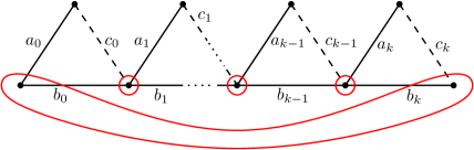
Figure 1. A bowtie ring. All elements are distinct.

A bowtie consists of a pair of disjoint triangles whose union contains a $4$-element cocircuit. Assume $k\geq 2$, and $T_{0},T_{1},\dots,T_{k}$ is a sequence of pairwise disjoint triangles. Let $T_{i}$ be $\{a_{i},b_{i},c_{i}\}$ for $i\in\{0,1,\ldots,k\}$. Assume $D_{i}=\{b_{i},c_{i},a_{i+1},b_{i+1}\}$ is a cocircuit for $i\in\{0,1,\ldots,k-1\}$, and in addition, $D_{k}=\{b_{k},c_{k},a_{0},b_{0}\}$ is a cocircuit. Then we say that $T_{0},D_{0},T_{1},D_{1},\dots,T_{k},D_{k}$ is a ring of bowties. Although the matroid $M$ we are dealing with need not be graphic, we follow the convention begun in [1] of using a modified graph diagram to keep track of some of the circuits and cocircuits in $M$. Figure 1 shows such a modified graph diagram. Each of the cycles in such a graph diagram corresponds to a circuit of $M$ while a circled vertex indicates a known cocircuit of $M$. If $M^{\prime}=M\backslash\{c_{0},c_{1},\dots,c_{k}\}$, then we say that $M^{\prime}$ is obtained from $M$ by trimming a ring of bowties.

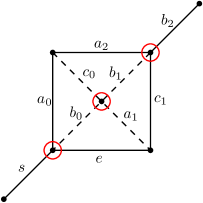
Figure 2. An augmented $4$-wheel. All displayed elements are distinct.

An augmented $4$-wheel is represented by the modified graph diagram in Figure 2, where the four dashed edges form the central cocircuit. If a matroid $M$ contains the structure in Figure 2 and $M\backslash e$ is $(4,4,S)$-connected, then we say that the augmented $4$-wheel is good. We refer to the operation of deleting the four dashed edges as removing the central cocircuit of an augmented $4$-wheel.

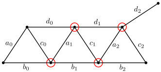
Figure 3. The elements shown are distinct.

Our third structure requires a special four-element move. If $M$ contains the structure in Figure 3, then we say that $M\backslash c_{1},c_{2}/d_{1},b_{2}$ is obtained from $M$ by a ladder-compression move.

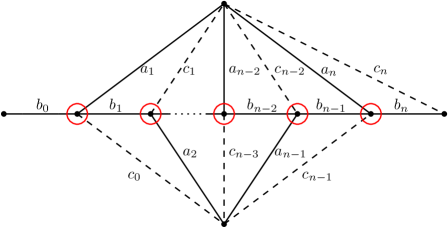
Figure 4. All the elements shown are distinct.

Finally, we consider the structure in Figure 4. Note that $n$ may be either even or odd. When there are at least three dashed elements, we refer to the structure in Figure 4 as an open rotor chain and we refer to the operation of deleting the dashed elements as trimming an open rotor chain.

3. The special graphs and matroids

This section has two purposes. First, we introduce all the graphs and matroids that feature in Theorem 1.1, which we now restate.

Theorem 3.1.

Assume that $(M_{0},N_{0})$ is a fascinating pair and $|E(M_{0})|\leq 15$. Then, for some pair, $(M,N)$ in $\{(M_{0},N_{0}),(M_{0}^{*},N_{0}^{*})\}$, one of the following statements holds.

1. $M$ is one of $M(Q_{3})$ or $M(K_{5})\cong M(\mathit{QM}_{5})$, and $N$ is $M(K_{4})$;

2. $M$ is one of $\Upsilon_{6}$ or $\Upsilon_{6}^{*}$, and $N$ is $F_{7}\cong\Upsilon_{4}^{*}$;

3. $M$ is one of $M(H_{1})$, $M(H_{2})$, $M(H_{3})$, or $M(\mathit{QM}_{7})$, and $N$ is $M(K_{3,3})\cong M(\mathit{CM}_{6})$;

4. $M$ is one of $M(Q_{3}^{\times})$, $M(Y_{9})$, $M(\mathit{QM}_{7})$, or $M(\mathit{CM}_{10})$, and $N$ is $M(K_{5})\cong M(\mathit{QM}_{5})$;

5. $M$ is one of $A_{1}$, $A_{2}$, $A_{3}$, $A_{4}$, $A_{5}$, $A_{6}$, or $\Upsilon_{8}$, and $N$ is $\Delta_{4}$;

6. $M$ is one of $B_{1}$, $B_{2}$, $B_{3}$, $B_{4}$, or $B_{5}$, and $N$ is $P$;

7. $M$ is one of $C_{1}$, $C_{2}$, $C_{3}$, or $C_{4}$, and $N$ is $Q$;

8. $(M,N)=(D_{1},R)$;

9. $(M,N)=(E_{1},S)$; or

10. $(M,N)=(\Upsilon_{8},\Upsilon_{6})$.

In many of the pairs from this theorem, it is possible to apply one of the four moves described in Section 2. Thus the second purpose of this section is to document these moves, and ultimately prove Theorem 1.4, which we restate next.

Theorem 3.2.

Let the pair $(M,N)$ be as described in one of the statements (1)–(10) in Theorem 1.1. If $(M,N)$ is not one of $(M(Q_{3}),M(K_{4}))$, $(M(K_{5}),M(K_{4}))$, $(\Upsilon_{6},F_{7})$, $(\Upsilon_{6}^{*},F_{7})$, $(M(\mathit{QM}_{7}),M(K_{3,3}))$, or $(\Upsilon_{8},\Delta_{4})$, then $N$ can be obtained from $M$ (or $N^{*}$ can be obtained from $M^{*}$) by one of the following four operations:

1. trimming a ring of bowties;

2. deleting the central cocircuit of a good augmented $4$-wheel;

3. a ladder-compression move; or

4. trimming an open rotor chain.

Now we start describing various graphs and matroids, beginning with the graphs $K_{4}$, $K_{5}$, and $Q_{3}$, all of which are illustrated in Figure 5. The graph $Q_{3}$ is also known as the cube graph. Figure 5 also shows the octahedron graph, $O$, which is the planar dual of $Q_{3}$.

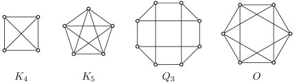
Figure 5. Graphs $K_{4}$, $K_{5}$, $Q_{3}$, and $O$.

In Lemma 2.3 of [10], Geelen and Zhou describe five internally $4$-connected graphs having $K_{3,3}\cong\mathit{CM}_{6}$ as a minor. One of the five is $\mathit{CM}_{8}$, which has only $12$ edges. Another is isomorphic to $\mathit{QM}_{7}$. Let the other three graphs be $H_{1}$, $H_{2}$, and $H_{3}$. These are shown in Figure 6.

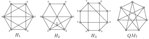
Figure 6. Graphs $H_{1}$, $H_{2}$, $H_{3}$, and $\mathit{QM}_{7}$.

Proposition 3.3.

Let $(M,N)$ be one of the pairs $(M(H_{1}),M(K_{3,3}))$, $(M(H_{2}),M(K_{3,3}))$, or $(M^{*}(H_{3}),M^{*}(K_{3,3}))$. Then $N$ is obtained from $M$ by trimming a bowtie ring, deleting the central cocircuit from a good augmented $4$-wheel, or a ladder-compression move.

Proof.

Note that $M(H_{1})$ has the bowtie ring shown in Figure 7, and trimming this ring yields $M(K_{3,3})$. Also, $M(H_{2})$ has a good augmented $4$-wheel whose central cocircuit is the set of edges incident with vertex $6$. Deleting this cocircuit yields $M(K_{3,3})$. Finally, $M^{*}(H_{3})$ has the ladder segment shown in Figure 3, where edges $(16,12,01,07,03,23,34,47,45,25,56,67)$ correspond to $(a_{0},b_{0},c_{0},d_{0},a_{1},b_{1},c_{1},d_{1},a_{2},b_{2},c_{2},d_{2})$. If we delete $c_{1}$ and $c_{2}$, and contract $d_{1}$ and $b_{2}$, then we obtain $M^{*}(K_{3,3})$. ∎

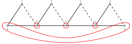
Figure 7. Bowtie ring in $H_{1}$.

Observe that of all the pairs in statements (1), (2), and (3) in Theorem 3.1 are either exceptional pairs that appear in Theorem 3.2, or are dealt with by Proposition 3.3. Thus we have verified Theorem 3.2 for these pairs.

The graphs $Q_{3}^{\times}$ and $Y_{9}$ are shown in Figure 8, along with $\mathit{CM}_{10}$.

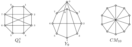
Figure 8. Graphs $Q_{3}^{\times}$, $Y_{9}$, and $\mathit{CM}_{10}$.

Proposition 3.4.

Let $(M,N)$ be one of the pairs $(M^{*}(Q_{3}^{\times}),M^{*}(K_{5}))$, $(M^{*}(Y_{9}),M^{*}(K_{5}))$, $(M(\mathit{QM}_{7}),M(K_{5}))$, or $(M^{*}(\mathit{CM}_{10}),M^{*}(K_{5}))$. Then $N$ is obtained from $M$ by trimming a bowtie ring, deleting the central cocircuit from a good augmented $4$-wheel, or a ladder-compression move.

Proof.

Figure 9 shows a labelling of some of the edges in $Q_{3}^{\times}$, along with a good augmented $4$-wheel in $M^{*}(Q_{3}^{\times})$. Deleting the central cocircuit of this augmented wheel produces $M^{*}(K_{5})$. Figure 10 shows the labelling of a bowtie ring in $M^{*}(Y_{9})$. Trimming this ring produces $M^{*}(K_{5})$. Similarly, by trimming the bowtie ring shown in Figure 11, we can obtain $M^{*}(K_{5})$ from $M^{*}(\mathit{CM}_{10})$. Finally, it is clear that $M(\mathit{QM}_{n-2})$ is obtained from $M(\mathit{QM}_{n})$ by a ladder-compression move, so in particular this applies to $M(\mathit{QM}_{7})$ and $M(\mathit{QM}_{5})\cong M(K_{5})$. ∎

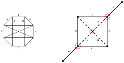
Figure 9. $Q_{3}^{\times}$ and a good augmented $4$-wheel in $M^{*}(Q_{3}^{\times})$.

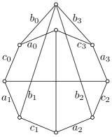
Figure 10. A bowtie ring in $M^{*}(Y_{9})$.

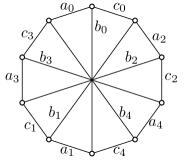
Figure 11. A bowtie ring in $M^{*}(\mathit{CM}_{10})$.

Since Proposition 3.4 verifies Theorem 3.2 for the pairs listed in statement (4) of Theorem 3.1, we now move to non-graphic binary matroids. We shall describe each of these matroids by giving a matrix that is a reduced binary representation for it. For example, Figure 12 shows a matrix, $A$, which is a reduced representation of $\Delta_{4}$. Figure 13 shows a geometric representation of $\Delta_{4}$. Note that the element $9$ corresponds to $\gamma$, so deleting $9$ produces a matroid isomorphic to $M^{*}(\mathit{CM}_{6})\cong M^{*}(K_{3,3})$.

Figure 12. Representations of $\Delta_{4}$ and $P$.

Figure 13. A geometric representation of $\Delta_{4}$.

The matroids $A_{1}$, $A_{2}$, $A_{3}$, $A_{4}$, and $A_{5}$ have as reduced representations the reduced matrices shown in Figure 14. Thus each of $A_{1}$, $A_{2}$, $A_{3}$, $A_{4}$, and $A_{5}$ is a rank-$8$ binary matroid with $14$ elements, and each contains a $4$-element independent set whose contraction produces a minor isomorphic to $\Delta_{4}$. The matroid $A_{6}$ is represented in Figure 15. We can produce a $\Delta_{4}$-minor from $A_{6}$ by contracting a $3$-element independent set and deleting a single element.

Figure 14. Representations of $A_{1}$, $A_{2}$, $A_{3}$, $A_{4}$, and $A_{5}$.

Figure 15. A representation of $A_{6}$.

Proposition 3.5.

Let $(M,N)$ be one of the pairs $(A_{1}^{*},\Delta_{4}^{*})$, $(A_{2}^{*},\Delta_{4}^{*})$, $(A_{3}^{*},\Delta_{4}^{*})$, $(A_{4}^{*},\Delta_{4}^{*})$, $(A_{5}^{*},\Delta_{4}^{*})$, or $(A_{6}^{*},\Delta_{4}^{*})$. Then $N$ is obtained from $M$ by trimming a bowtie ring, trimming an open rotor chain, or deleting the central cocircuit from a good augmented $4$-wheel.

Proof.

We will check that $\Delta_{4}^{*}$ is obtained from each of $A_{1}^{*},A_{2}^{*},A_{3}^{*}$, and $A_{5}^{*}$ by trimming a bowtie ring. In Figure 14, assume that the matrices inherit the labels on rows and columns from $A$, so that the first four rows of any matrix are labelled $0$, $1$, $2$, $3$, the columns are labelled $4$, $5$, $6$, $7$, $8$, $9$, and the last four rows are labelled $10$, $11$, $12$, and $13$. Now $A_{1}^{*}$ contains a bowtie ring, as in Figure 1, where $n=3$, and the labelling puts

$$(a_{0},b_{0},c_{0},a_{1},b_{1},c_{1},\dots,a_{3},b_{3},c_{3})=(3,0,10,9,2,12,1,5,11,8,7,13).$$

Trimming this ring produces $\Delta_{4}^{*}$. Similar statements apply to $A_{2}^{*},A_{3}^{*}$, and $A_{5}^{*}$. In those cases, the bowtie rings, $(a_{0},b_{0},c_{0},a_{1},b_{1},c_{1},\dots,a_{3},b_{3},c_{3})$, are

$$(4,8,11,5,7,12,0,3,10,2,6,13),\quad(4,6,10,3,2,12,1,5,11,7,8,13),\\ \text{and}\quad(1,0,12,2,9,11,7,6,13,8,4,10).$$

The matroid $A_{4}^{*}$ contains an open rotor chain, as in Figure 4, where $n=3$, and we label so that

$$(b_{0},c_{0},a_{1},b_{1},c_{1},a_{2},b_{2},c_{2},a_{3},b_{3},c_{3})=(2,10,3,6,13,4,8,11,7,5,12).$$

Trimming this rotor chain produces $\Delta_{4}^{*}$.

Finally, for $A_{6}$, we assume the matrix in Figure 15 inherits the labels from $A$, and we label the extra column $10$, and the extra rows as $11,12$, and $13$. Then $A_{6}^{*}$ contains an augmented $4$-wheel, as in Figure 2, where we label so that $(e,s,a_{0},b_{0},c_{0},a_{1},b_{1},c_{1},a_{2},b_{2})$ are replaced by $(1,0,13,10,4,11,12,5,8,7)$. Now $A_{6}^{*}\backslash 1$ is $(4,4,S)$-connected, and $A_{6}^{*}\backslash 4,10,11,12\cong\Delta_{4}^{*}$, so the proof of the proposition is complete. ∎

Before we continue, we recall some introductory material. A simple rank-$r$ binary matroid, $M$, can be considered as a subset, $E$, of points in the projective geometry $\mathrm{PG}(r-1,2)$. The complement of $M$ is the binary matroid corresponding to the set of points of $\mathrm{PG}(r-1,2)$ not in $E$. The complement of $M$ is well-defined by [15, Proposition 10.1.7], meaning that it depends only on $M$, and not on the choice of $E$. In particular, if two simple rank-$r$ binary matroids have isomorphic complements, then they are themselves isomorphic. The complement of $M^{*}(K_{3,3})$ in $\mathrm{PG}(3,2)$ is $U_{2,3}\oplus U_{2,3}$, and the complement of $\Delta_{4}$ is $U_{2,2}\oplus U_{2,3}$. The complement of $M(K_{5})$ in $\mathrm{PG}(3,2)$ is $U_{4,5}$. From this, it follows that $M(K_{5})$ has a unique simple rank-$4$ binary extension on $11$ elements. We denote this extension by $P$, so the complement of $P$ is $U_{4,4}$. The matrix $B$, shown in Figure 12, represents $P$ over $\mathrm{GF}(2)$. Note that $P\backslash 10$ is isomorphic to $M(K_{5})$, and that $10$ is in triangles with $\{4,9\}$, $\{5,8\}$, and $\{6,7\}$, where each of these pairs corresponds to a matching in $K_{5}$. The matroids $B_{1}$, $B_{2}$, $B_{3}$, $B_{4}$, and $B_{5}$ are represented by the matrices in Figure 16.

Figure 16. Representations of $B_{1}$, $B_{2}$, $B_{3}$, $B_{4}$, and $B_{5}$.

Proposition 3.6.

Let $(M,N)$ be one of the pairs $(B_{1}^{*},P^{*})$, $(B_{2}^{*},P^{*})$, $(B_{3}^{*},P^{*})$, $(B_{4}^{*},P^{*})$, $(B_{5}^{*},P^{*})$. Then $N$ is obtained from $M$ by trimming a bowtie ring.

Proof.

We assume that each matrix, $B_{i}$, inherits the labels on $B$, and that the extra rows are labelled $11$, $12$, $13$, and $14$. In $B_{1}^{*}$, there is a bowtie ring, as in Figure 1, with $n=3$, where $(a_{0},b_{0},c_{0},a_{1},b_{1},c_{1},a_{2},b_{2},c_{2},a_{3},b_{3},c_{3})$ is relabelled as $(1,3,12,0,6,11,5,9,13,7,8,14)$. Similarly, for $B_{2}^{*}$, $B_{3}^{*}$, $B_{4}^{*}$, and $B_{5}^{*}$, the relevant relabellings are $(1,8,12,10,5,13,2,0,11,6,3,14)$, $(8,5,13,0,2,11,3,9,14,4,10,12)$, $(10,8,14,3,1,11,0,4,12,7,5,13)$, and $(8,1,12,7,2,13,5,0,11,6,3,14)$. ∎

Let $Q$ be the binary matroid represented by the matrix $C$, below. Note that $Q$ is obtained by extending $\Delta_{4}$ by the element $10$ in such a way that $\{0,8,10\}$ is a triangle. The complement of $Q$ in $\mathrm{PG}(3,2)$ is $U_{1,1}\oplus U_{2,3}$.

The matroids $C_{1}$, $C_{2}$, $C_{3}$, and $C_{4}$ are represented by the matrices in Figure 17.

Figure 17. Representations of $C_{1}$, $C_{2}$, $C_{3}$, and $C_{4}$.

Proposition 3.7.

Let $(M,N)$ be one of the pairs $(C_{1}^{*},Q^{*})$, $(C_{2}^{*},Q^{*})$, $(C_{3}^{*},Q^{*})$, $(C_{4}^{*},Q^{*})$. Then $N$ is obtained from $M$ by trimming a bowtie ring.

Proof.

We assume that each matrix $C_{i}$ inherits the row and column labels from $C$, and the extra rows are labelled $11$, $12$, $13$, and $14$. We relabel the elements $(a_{0},b_{0},c_{0},a_{1},b_{1},c_{1},a_{2},b_{2},c_{2},a_{3},b_{3},c_{3})$ in Figure 1 $(1,6,12,7,9,13,2,0,11,8,10,14)$ for $C_{1}^{*}$, $(4,9,12,2,0,11,3,7,14,8,5,13)$ for $C_{2}^{*}$, $(9,4,12,8,6,14,1,10,11,3,5,13)$ for $C_{3}^{*}$, and $(7,0,11,4,1,12,5,2,13,6,3,14)$ for $C_{4}^{*}$. ∎

Propositions 3.5, 3.6 and 3.7 verify Theorem 3.2 for the pairs listed in statements (5), (6), and (7) in Theorem 3.1. There are two matrices in Figure 18. The matrix $D$ represents the binary matroid $R$. Note that $R$ is obtained from $M(K_{5})$ by coextending by the element $10$ so that $10$ is in a triad with two elements that correspond to a $2$-edge matching in $K_{5}$. Therefore $R$ is isomorphic to the matroid obtained from $P$ by performing a $\Delta\text{-}Y$-operation on the triangle $\{4,9,10\}$.

Figure 18. Representations of $R$ and $D_{1}$.

Proposition 3.8.

$R^{*}$ can be obtained from $D_{1}^{*}$ by trimming a bowtie ring.

Proof.

Label the extra rows in $D_{1}$ that are not in $D$ as $11$, $12$, $13$, and $14$. Then $(8,3,12,6,0,11,5,2,13,7,1,14)$ is the appropriate bowtie ring. ∎

The matroid $S$ is represented by the matrix $E$, and $E_{1}$ is represented by the matrix shown in Figure 19. We can obtain $S$ from $\Delta_{4}$ by coextending by the element $10$ so that it is in a triad with $0$ and $8$. Thus $S$ can also be obtained from $Q$ by a $\Delta\text{-}Y$-operation.

Figure 19. Representations of $S$ and $E_{1}$.

Proposition 3.9.

$S^{*}$ can be obtained from $E_{1}^{*}$ by trimming a bowtie ring.

Proof.

Label the extra rows in $E_{1}$ that are not in $E$ as $11$, $12$, $13$, and $14$. Then $(1,5,11,4,9,12,7,6,14,3,2,13)$ is the appropriate bowtie ring. ∎

Recall that the Möbius matroids are defined in Section 1.

Proposition 3.10.

When $r\geq 6$ is an even integer, the matroid $\Upsilon_{r}^{*}$ can be obtained from $\Upsilon_{r+2}^{*}$ by a ladder-compression move.

Proof.

Recall that $\Upsilon_{r+2}^{*}=M_{r+1}$ and $\Upsilon_{r}^{*}=M_{r-1}$, where $M_{k}$ is an extension of the rank-$k$ wheel by the element $\gamma$. Assume that the spokes of $M({\mathcal{W}}_{r+1})$, in cyclic order, are $x_{0},x_{1},\ldots,x_{r}$ and that $\{x_{i},y_{i},x_{i+1}\}$ is a triangle of $M({\mathcal{W}}_{r+1})$ for $i=0,1,\ldots,r$. (We interpret subscripts modulo $r+1$.) Then, for $i=0,1,\ldots,r$, the set $\{y_{i},x_{i+1},y_{i+1},\gamma\}$ is a cocircuit of $M_{r+1}$. We obtain $M_{r-1}$ from $M_{r+1}$ by contracting $y_{r-1}$ and $y_{r}$, and deleting $x_{r-1}$ and $x_{0}$, and then relabelling $x_{r}$ as $x_{0}$. To see this, observe that $M_{r+1}$ has $\{x_{0},\ldots,x_{r},\gamma\}$ and $\{x_{r-1},x_{r},y_{r-1}\}$ as circuits, so their symmetric difference, $C=\{x_{0},\ldots,x_{r-2},y_{r-1},\gamma\}$, is a disjoint union of circuits. Orthogonality with the cocircuits containing $\gamma$ implies that $C$ is a circuit of $M_{r+1}$. Next we note that $\{x_{r-1},x_{r},y_{r-2},y_{r}\}$ is the symmetric difference of $\{y_{r-2},x_{r-1},y_{r-1},\gamma\}$ and $\{y_{r-1},x_{r},y_{r},\gamma\}$, and is therefore a disjoint union of cocircuits. This implies that $y_{r}$ is not in the closure of $C$ in $M_{r+1}$. Therefore $C-y_{r-1}=\{x_{0},\ldots,x_{r-2},\gamma\}$ is a spanning circuit of $M_{r+1}/y_{r-1},y_{r}\backslash x_{r-1},x_{0}$, and it follows easily that this matroid is $M_{r-1}$, up to relabelling.

Now we need only show that this operation is a ladder-compression move. We note that $M_{r+1}$ contains a ladder segment, as depicted in Figure 3, where the labels $a_{0}$, $b_{0}$, $c_{0}$, $d_{0}$, $a_{1}$, $b_{1}$, $c_{1}$, $d_{1}$, $a_{2}$, $b_{2}$, $c_{2}$, and $d_{2}$ are replaced by $x_{r-4}$, $y_{r-4}$, $x_{r-3}$, $y_{r-3}$, $x_{r-2}$, $y_{r-2}$, $x_{r-1}$, $y_{r-1}$, $x_{r}$, $y_{r}$, $x_{0}$, and $y_{0}$, respectively. Because $r\geq 6$, these elements are all distinct. ∎

Proposition 3.10 now implies that $\Upsilon_{6}^{*}$ can be obtained from $\Upsilon_{8}^{*}$ by a ladder-compression move. Thus we have completed the proof of Theorem 1.4.

Proof of Corollary 1.5..

If $(M,N)$ is $(M(\mathit{QM}_{7}),M(K_{4}))$, then we can set $M_{0}$ to be $M(\mathit{QM}_{5})\cong M(K_{5})$, and $M_{0}$ can be obtained from $M$ by a ladder-compression move. If $(M,N)$ is $(\Upsilon_{8},F_{7})$ or $(\Upsilon_{8}^{*},F_{7})$, then we can set $M_{0}$ to be $\Upsilon_{6}$ or $\Upsilon_{6}^{*}$, respectively. In either case, by Proposition 3.10, we can use a ladder-compression move to obtain $M_{0}^{*}$ from $M^{*}$ (in the first case), or $M_{0}$ from $M$ (in the second). ∎

4. Proof of the main results

We prove Theorem 1.1. Assume that $(M,N)$ is a fascinating pair that contradicts the statement of the theorem.

4.1.1.

$|E(N)|\in\{10,11\}$.

Certainly $|E(N)|\leq 11$, since $|E(M)|\leq 15$, and $(M,N)$ is a fascinating pair, so $|E(M)|-|E(N)|>3$. Assume that $|E(N)|<10$. First consider the case that $|E(N)|=6$, so that $N$ is isomorphic to $M(K_{4})$. If $M$ has a proper minor, $M^{\prime}$, such that $|E(M)|-|E(M^{\prime})|\leq 3$, and $M^{\prime}$ is internally $4$-connected, then $M^{\prime}$ has an $M(K_{4})$-minor [16, Corollary 12.2.13], and hence $(M,N)$ is not a fascinating pair. Therefore $M$ has no such minor, so we can apply our chain theorem [1, Theorem 1.3]. Since $|E(M)|\leq 15$, it follows from that theorem that $M$ is the cycle matroid of a planar or Möbius quartic ladder, or the dual of such a matroid. The only planar quartic ladder with fewer than $16$ edges is the octahedron, $O$, which is the dual graph of $Q_{3}$, the cube. The only Möbius quartic ladders with fewer than $16$ edges have $14$ or $10$ edges. The former has the latter as a minor, and the latter is isomorphic to $K_{5}$. From this we deduce that, up to duality, $(M,N)$ is $(M(Q_{3}),M(K_{4}))$ or $(M(K_{5}),M(K_{4}))$, and that therefore $(M,N)$ is not a counterexample after all. Hence $6<|E(N)|<10$. The only internally $4$-connected binary matroids satisfying this constraint are $F_{7}$, $M(K_{3,3})$, and their duals. (This fact is [10, Lemma 2.1], and will also be confirmed by the subsequent exhaustive search.) Thus we can assume $N$ is $F_{7}$ or $M(K_{3,3})$.

From this point, we use almost exactly the same arguments as in [4, Lemma 2.3]. Assume $N$ is $F_{7}$, so $|E(M)|\geq 11$. We can use [18, Corollary 1.2] to deduce that $M$ is isomorphic to $T_{12}\backslash e\cong\Upsilon_{6}$ or $T_{12}/e\cong\Upsilon_{6}^{*}$, so $(M,N)$ fails to contradict the theorem. Therefore we assume $N$ is $M(K_{3,3})$, and hence $|E(M)|\geq 13$. Now we can use [10, Lemma 2.3]. This lemma defines five graphs, but only four of them have at least $13$ edges. Therefore we can deduce that $M$ is isomorphic to one of the graphic matroids $M(H_{1})$, $M(H_{2})$, $M(H_{3})$, or $M(\mathit{QM}_{7})$. Again this is a contradiction, as it implies that $(M,N)$ is not a counterexample, so the proof of 4.1.1 is complete.

At this point, it is appropriate to verify that the pairs mentioned in the proof of 4.1.1 are indeed fascinating. We do this, and the rest of the search, using the matroid capabilities of sage (Version 6.10). First we want to allow access to certain special functions of the sage matroids package.

from sage.matroids.advanced import *

We will require a test for internal $4$-connectivity.

def IsIFC(M):
    if len(M)<=7:
        return True
    elif len(M)==8 or len(M)==9:
        return all( (M.rank(X)+
             M.rank(M.groundset().symmetric_difference(X))-
             M.rank() > 2) for X in Subsets(M.groundset(),4) )
    elif len(M)==10 or len(M)==11:
        return all( (M.rank(X)+
            M.rank(M.groundset().symmetric_difference(X))-
            M.rank() > 2) for X in Subsets(M.groundset(),4) )
            and all( (M.rank(X)+
            M.rank(M.groundset().symmetric_difference(X))-
            M.rank() > 2) for X in Subsets(M.groundset(),5) )
    elif len(M)==12 or len(M)==13:
        return all( (M.rank(X)+
            M.rank(M.groundset().symmetric_difference(X))-
            M.rank() > 2) for X in Subsets(M.groundset(),4) )
            and all( (M.rank(X)+
            M.rank(M.groundset().symmetric_difference(X))-
            M.rank() > 2) for X in Subsets(M.groundset(),5) )
            and all( (M.rank(X)+
            M.rank(M.groundset().symmetric_difference(X))-
            M.rank() > 2) for X in Subsets(M.groundset(),6) )
    elif len(M)==14 or len(M)==15:
        return all( (M.rank(X)+
            M.rank(M.groundset().symmetric_difference(X))-
            M.rank()>2) for X in Subsets(M.groundset(),4) )
            and all( (M.rank(X)+
            M.rank(M.groundset().symmetric_difference(X))-
            M.rank() > 2) for X in Subsets(M.groundset(),5) )
            and all( (M.rank(X)+
            M.rank(M.groundset().symmetric_difference(X))-
            M.rank() > 2) for X in Subsets(M.groundset(),6) )
            and all( (M.rank(X)+
            M.rank(M.groundset().symmetric_difference(X))-
            M.rank() > 2) for X in Subsets(M.groundset(),7) )

This command works for $3$-connected matroids with a ground set of size $n$, where $0\leq n\leq 15$. For each such $n$, the command considers each subset, $X$, of size between $4$ and $\lfloor n/2\rfloor$, and checks that $r(X)+r(E(M)-X)-r(M)>2$. If this is the case, it returns True, and otherwise it returns False.

Next we define a function that will test whether a pair $(M,N)$ is fascinating. In the following code, and elsewhere, note that the command range(n) produces the list $[0,1,2,\ldots,n-1]$, and range(m,n) produces $[m,m+1,\ldots,n-1]$.

def Fascinating(M,N):
    rankgap=M.rank()-N.rank()
    sizegap=len(M)-len(N)
    if sizegap>3 and M.has_minor(N):
        Between=False
        for r in range(rankgap+1):
            if Between:
                break
            for F in M.flats(r):
                if Between:
                    break
                if len(F)<sizegap and M.contract(F).has_minor(N):
                    if r==0:
                        Lower=1
                    else:
                        Lower=0
                    DeleteSet=M.groundset().difference(F)
                    for i in range(Lower,sizegap-len(F)):
                        if Between:
                            break
                        for D in Subsets(DeleteSet,i):
                            Test=M.contract(F).delete(D)
                            if Test.has_minor(N):
                                if Test.is_3connected()
                                    and IsIFC(Test):
                                       Between=True
                                       break
        return not Between
    else:
        return False

First the function tests that $M$ has an $N$-minor and $|E(M)|-|E(N)|>3$. If this is not the case, it returns False. Otherwise, it considers all flats, $F$, of $M$ such that $0\leq r(F)\leq r(M)-r(N)$. If $M/F$ has a proper $N$-minor, then it considers subsets, $D$, of $E(M/F)$. If $F$ is the rank-$0$ flat (which we assume to be empty), then $D$ is constrained to contain at least one element. In any case, $D$ is constrained so that $|D|<|E(M)|-|E(N)|-|F|$. Thus $D$ ranges over all subsets such that $|E(N)|<|E(M/F\backslash D)|<|E(M)|$. If $M/F\backslash D$ is internally $4$-connected and has an $N$-minor, then the Boolean value Between is set to be True. At any time, if Between is found to be True, then the function breaks out of the loop. Finally, it returns the negation of Between.

Now we can test the pairs that have arisen in the proof up to this point.

K4=matroids.CompleteGraphic(4)
K5=matroids.CompleteGraphic(5)
Q3=Matroid(graph=graphs.CubeGraph(3))
F7=matroids.named_matroids.Fano()
Upsilon6=matroids.named_matroids.T12().delete(’e’)
K33=Matroid(graph=graphs.CompleteBipartiteGraph(3,3))
H1=Matroid(graph=Graph({0:[1,2,4,5],1:[2,3,4,5],2:[3,4],
   3:[4,5],4:[5]}))
H2=Matroid(graph=Graph({0:[1,3,5],1:[2,4,6],2:[3,5,6],
   3:[4,6],4:[5,6]}))
H3=Matroid(graph=Graph({0:[1,3,7],1:[2,6],2:[3,5,7],
   3:[4],4:[5,7],5:[6],6:[7]}))
QML7=Matroid(graph=graphs.CirculantGraph(7,[1,3,4]))

print Fascinating(K5,K4)
print Fascinating(Q3,K4)
print Fascinating(Upsilon6,F7)
print Fascinating(Upsilon6.dual(),F7)
print Fascinating(H1,K33)
print Fascinating(H2,K33)
print Fascinating(H3,K33)
print Fascinating(QML7,K33)
    True
    True
    True
    True
    True
    True
    True
    True

By duality, we may assume that $r(M)\leq r^{*}(M)$. As $|E(M)|\leq 15$, the next result is a consequence.

4.1.2.

$r(N)\leq r(M)\leq 7$.

We create an object that will contain the catalogue of all $3$-connected binary matroids with ground sets of cardinality between $6$ and $15$ and rank at most $7$. This object is a library, containing 10 lists, each indexed by an integer between $6$ and $15$. Each list itself contains eight lists, indexed by integers between $0$ and $7$. Thus, if $6\leq n\leq 15$, and $0\leq r\leq 7$, then Catalogue[n][r] is the list indexed by $r$, contained in the list indexed by $n$; that is, it is the list of all $3$-connected binary matroids with rank $r$ and a ground set of size $n$. We initialise by creating empty lists.

Catalogue={}
for i in range(6,16):
    Catalogue[i]=[[] for j in range(0,8)]

Every $3$-connected binary matroid with at least $6$ elements contains an $M(K_{4})$-minor [16, Corollary 12.2.13]. We are going to populate our catalogue by starting with this matroid, and enlarging the catalogue through single-element extensions and coextensions. When we extend, we ensure we produce no coloops, no loops, and no parallel pairs. Dually, when we coextend, we create no loops, coloops, or series pairs. Thus we only ever create $3$-connected matroids [15, Proposition 8.1.10]. Every $3$-connected binary matroid can be constructed in this way, with the exception of wheels [16, Theorem 8.8.4], so we manually input the wheels of rank $3$, $4$, $5$, $6$, and $7$. In this way, we guarantee that our catalogue will contain every $3$-connected binary matroid with suitable size and rank.

Wheel3=Matroid(reduced_matrix=Matrix(GF(2),[[1,0,1],[1,1,0],
    [0,1,1]]))
Wheel4=Matroid(reduced_matrix=Matrix(GF(2),[[1,0,0,1],
    [1,1,0,0],[0,1,1,0],[0,0,1,1]]))
Wheel5=Matroid(reduced_matrix=Matrix(GF(2),[[1,0,0,0,1],
    [1,1,0,0,0],[0,1,1,0,0],[0,0,1,1,0],[0,0,0,1,1]]))
Wheel6=Matroid(reduced_matrix=Matrix(GF(2),[[1,0,0,0,0,1],
    [1,1,0,0,0,0],[0,1,1,0,0,0],[0,0,1,1,0,0],[0,0,0,1,1,0],
    [0,0,0,0,1,1]]))
Wheel7=Matroid(reduced_matrix=Matrix(GF(2),[[1,0,0,0,0,0,1],
    [1,1,0,0,0,0,0],[0,1,1,0,0,0,0],[0,0,1,1,0,0,0],
    [0,0,0,1,1,0,0],[0,0,0,0,1,1,0],[0,0,0,0,0,1,1]]))

Now we seed our catalogue by adding the wheels.

Catalogue[6][3].append(Wheel3)
Catalogue[8][4].append(Wheel4)
Catalogue[10][5].append(Wheel5)
Catalogue[12][6].append(Wheel6)
Catalogue[14][7].append(Wheel7)

At any time, we can save our current catalogue with a command of the following type.

save (Catalogue, "/SampleFolder/catalogue.sobj")

We are then able to recover our saved work with the following command.

Catalogue = load("/SampleFolder/catalogue.sobj")

Now we define the command Populate, which we will use to fill in the entries in our catalogue. On input $n$, the command fills in all entries of the catalogue corresponding to matroids with ground sets of size $n$. It does this by letting the rank, $r$, range from $0$ to $7$, and considering all matroids of rank $r$ in the catalogue of matroids with ground sets of size $n-1$. For each such matroid, $N$, it generates the list of non-isomorphic simple single-element extensions of $N$, using the built-in command get_nonisomorphic_matroids. It then adds these extensions to the catalogue of rank-$r$, size-$n$ matroids, as long as they are not isomorphic to matroids already appearing there. If $r$ is greater than zero, it then performs the same actions using cosimple single-element coextensions. Finally, it prints the number of matroids it has generated.

def Populate(n):
    for r in range(8):
        for N in Catalogue[n-1][r]:
            List=N.linear_extensions(simple=True,element=len(N))
            List=get_nonisomorphic_matroids(List)
            for M in List:
                if not any(L.is_isomorphic(M) for
                    L in Catalogue[n][r]):
                    Catalogue[n][r].append(M)
        if r>0:
            for N in Catalogue[n-1][r-1]:
                List=N.linear_coextensions(cosimple=True,
                        element=len(N))
                List=get_nonisomorphic_matroids(List)
                for M in List:
                    if not any(L.is_isomorphic(M) for
                        L in Catalogue[n][r]):
                        Catalogue[n][r].append(M)
    print [len(Catalogue[n][r]) for r in range(8)]

Generating the catalogue of $3$-connected binary matroids up to size $13$ takes only a few minutes.

%time
Populate(7)
    [0, 0, 0, 1, 1, 0, 0, 0]
    CPU time: 0.00 s,  Wall time: 0.00 s

%time
Populate(8)
    [0, 0, 0, 0, 3, 0, 0, 0]
    CPU time: 0.01 s,  Wall time: 0.01 s

%time
Populate(9)
    [0, 0, 0, 0, 4, 4, 0, 0]
    CPU time: 0.03 s,  Wall time: 0.03 s

%time
Populate(10)
    [0, 0, 0, 0, 4, 16, 4, 0]
    CPU time: 0.20 s,  Wall time: 0.20 s

%time
Populate(11)
    [0, 0, 0, 0, 3, 37, 37, 3]
    CPU time: 1.97 s,  Wall time: 1.97 s

%time
Populate(12)
    [0, 0, 0, 0, 2, 68, 230, 68]
    CPU time: 18.58 s,  Wall time: 18.58 s

%time
Populate(13)
    [0, 0, 0, 0, 1, 98, 983, 983]
    CPU time: 218.23 s,  Wall time: 218.26 s

Generating matroids with $14$ and $15$ elements takes considerably more time.

%time
Populate(14)
    [0, 0, 0, 0, 1, 121, 3360, 10035]
    CPU time: 3243.90 s,  Wall time: 3243.96 s

%time
Populate(15)
    [0, 0, 0, 0, 1, 140, 10012, 81218]
    CPU time: 83469.47 s,  Wall time: 83468.83 s

Now we work through our catalogue of all $3$-connected binary matroids, and pick out those that are internally $4$-connected. As before, we create an object that will be our catalogue of internally $4$-connected matroids.

IFCCatalogue={}
for i in range(6,16):
    IFCCatalogue[i]=[[] for j in range(0,8)]

We construct a command that will populate our catalogue with internally $4$-connected matroids.

def PopulateIFC(n):
    for r in range(8):
        for M in Catalogue[n][r]:
            if IsIFC(M):
                IFCCatalogue[n][r].append(M)
    print [len(IFCCatalogue[n][r]) for r in range(8)]

These are the results when we apply the command to fill our catalogue.

%time
PopulateIFC(6)
    [0, 0, 0, 1, 0, 0, 0, 0]
    CPU time: 0.00 s,  Wall time: 0.00 s

%time
PopulateIFC(7)
    [0, 0, 0, 1, 1, 0, 0, 0]
    CPU time: 0.00 s,  Wall time: 0.00 s

%time
PopulateIFC(8)
    [0, 0, 0, 0, 0, 0, 0, 0]
    CPU time: 0.00 s,  Wall time: 0.00 s

%time
PopulateIFC(9)
    [0, 0, 0, 0, 1, 1, 0, 0]
    CPU time: 0.02 s,  Wall time: 0.02 s

Since $F_{7}$ and $M(K_{3,3})$ are internally $4$-connected, from these commands it follows that, as stated earlier, the only internally $4$-connected binary matroids with seven, eight, or nine elements are $F_{7}$, $M(K_{3,3})$, and their duals.

%time
PopulateIFC(10)
    [0, 0, 0, 0, 2, 2, 2, 0]
    CPU time: 0.14 s,  Wall time: 0.14 s

%time
PopulateIFC(11)
    [0, 0, 0, 0, 2, 7, 7, 2]
    CPU time: 0.76 s,  Wall time: 0.78 s

%time
PopulateIFC(12)
    [0, 0, 0, 0, 2, 24, 46, 24]
    CPU time: 9.60 s,  Wall time: 9.60 s

%time
PopulateIFC(13)
    [0, 0, 0, 0, 1, 52, 272, 272]
    CPU time: 94.84 s,  Wall time: 94.87 s

%time
PopulateIFC(14)
    [0, 0, 0, 0, 1, 84, 1389, 3385]
    CPU time: 1829.54 s,  Wall time: 1829.78 s

%time
PopulateIFC(15)
    [0, 0, 0, 0, 1, 116, 5816, 36962]
    CPU time: 26298.59 s,  Wall time: 26297.77 s

These computations show that there are exactly $24$ internally $4$-connected binary matroids with ground sets of cardinality $10$ or $11$. We put these matroids into a list of possible “target” matroids:

Targets=[]
Targets.extend(IFCCatalogue[10][4])
Targets.extend(IFCCatalogue[10][5])
Targets.extend(IFCCatalogue[10][6])
Targets.extend(IFCCatalogue[11][4])
Targets.extend(IFCCatalogue[11][5])
Targets.extend(IFCCatalogue[11][6])
Targets.extend(IFCCatalogue[11][7])

We wish to process each of the internally $4$-connected matroids in our catalogue with a ground set of cardinality $11$, $12$, $13$, or $14$, and record which of the $24$ “target” matroids it has as a proper minor. We start by creating a new list of lists of lists.

TargetMinors={}
for n in range(11,15):
    TargetMinors[n]={}
    for r in range(8):
        TargetMinors[n][r]={}
        for i in range(len(IFCCatalogue[n][r])):
            TargetMinors[n][r][i]=[0 for j in range(24)]

Assume that $n$ is in $\{11,12,13,14\}$, $r$ is in $\{0,\ldots,7\}$, and $i$ indexes an internally $4$-connected matroid in the list IFCCatalogue[n][r]. The object TargetMinors[n][r][i] is a list with $24$ entries, each equal to $0$ or $1$. The entry TargetMinors[n][r][i][j] will be equal to $1$ if and only if matroid number $i$ in the list IFCCatalogue[n][r] contains a proper minor isomorphic to matroid number $j$ in the list Targets.

%time
for n in range(11,15):
    for r in range(8):
        for i in range(len(IFCCatalogue[n][r])):
            M=IFCCatalogue[n][r][i]
            for j in range(24):
                N=Targets[j]
                if len(N)<len(M) and M.has_minor(N):
                    TargetMinors[n][r][i][j]=1
    CPU time: 1797.00 s,  Wall time: 1797.06 s

The heart of the computer search is contained in the following code:

%time
for r in range(8):
    for i in range(len(IFCCatalogue[15][r])):
        M=IFCCatalogue[15][r][i]
        Possibles=set(range(24))
        for k in range(24):
            if not M.has_minor(Targets[k]):
                Possibles.discard(k)
        for size in range(14,10,-1):
            if len(Possibles)==0:
                break
            for rank in range(r,max(r-(15-size),0)-1,-1):
                if len(Possibles)==0:
                    break
                for j in range(len(IFCCatalogue[size][rank])):
                    Test=False
                    for k in Possibles:
                        if TargetMinors[size][rank][j][k]==1:
                            Test=True
                            break
                    if Test:
                        if M.has_minor(IFCCatalogue[size][rank][j]):
                            for k in range(24):
                                if TargetMinors[size][rank][j][k]==1:
                                    Possibles.discard(k)
                            if len(Possibles)==0:
                                break
        for k in Possibles:
            print (15,r,i,k)

This code lets the variable $r$ range between $0$ and $7$. For each $r$, the variable $i$ indexes a matroid, $M$, contained in the list IFCCatalogue[15][r], and $M$ ranges over all matroids in this list. We are trying to determine if there is an fascinating pair, $(M,N)$, that acts as a counterexample to the theorem. Recall that 4.1.1 implies that $|E(N)|$ is $10$ or $11$, and Targets contains a list of the $24$ matroids with $10$ or $11$ elements that could possibly be $N$. When processing $M$, we set Possibles to initially be $\{0,1,\ldots,23\}$. This set will record the indices of matroids in Target that can possibly be $N$. If $M$ does not contain a minor isomorphic to Targets[k], then we discard $k$ from Possibles. Indeed, throughout the process, we seek to discard indices from Possibles. If at any time, there are no indices left in Possibles, then we know that $M$ cannot be in the fascinating pair we seek, so we move to the next matroid. Assuming that Possibles is not empty, we let size range between $14$ and $11$ (starting at $14$), and we let rank range between $r$ and $r-(15-\texttt{size})$. We seek internally $4$-connected matroids with the parameters size and rank that are proper minors of $M$. (This is why we do not allow rank to be less than $r-(15-\texttt{size})$, since no minor of $M$ with ground set of cardinality size can have rank lower than this.) Now we let $j$ index a matroid in the list IFCCatalogue[size][rank]. Let the indexed matroid be $M^{\prime}$. If $M^{\prime}$ has no minor isomorphic to Targets[k], for any $k$ in Possibles, then we will not be able to use $M^{\prime}$ to discard any more indices in Possibles. So if this is the case, we do not consider $M^{\prime}$ any further. On the other hand, as soon as we find a $k$ in Possibles such that $M^{\prime}$ has a minor isomorphic to Targets[k], we move to the next stage of the process. In this stage, we first of all test that $M$ has an $M^{\prime}$-minor. In the case that it does, we let $k$ range through all of the indices in $\{0,1,\ldots,23\}$. If TargetMinors[size][rank][j][k] is $1$, indicating that $M^{\prime}$ has a minor isomorphic to Targets[k], then we can discard $k$ from Possibles, since the matroid $M^{\prime}$ means that no fascinating pair can contain $M$ and Targets[k]. We continue this process until either Possibles is empty, or until we have examined every possible matroid $M^{\prime}$. If Possibles is not empty at this stage, we know that, for every $k$ in Possibles, $(M,\texttt{Targets[k]})$ is a fascinating pair, so we print out the information (15,r,i,k), enabling us to identify the matroids in that pair.

Evaluating this command gives the following output:

(15, 6, 445, 5)
(15, 6, 589, 19)
(15, 6, 5414, 16)
(15, 7, 0, 4)
(15, 7, 0, 8)
(15, 7, 34137, 22)
(15, 7, 34466, 22)
(15, 7, 34693, 22)
(15, 7, 34762, 22)
(15, 7, 34769, 22)
(15, 7, 35415, 23)
(15, 7, 35441, 23)
(15, 7, 35445, 23)
(15, 7, 35455, 23)
CPU time: 77608.72 s,  Wall time: 77606.78 s

We now seek to find the fascinating pairs, $(M,N)$, where $|E(M)|=14$. This implies that $|E(N)|=10$. Since the only matroids in the list Targets with ground sets of cardinality $10$ are those with indices in $\{0,1,\ldots,5\}$, we change the code so that Possibles is initially set to $\{0,1,\ldots,5\}$. We also let size range between $13$ and $11$, instead of $14$ and $11$.

%time
for r in range(8):
    for i in range(len(IFCCatalogue[14][r])):
        M=IFCCatalogue[14][r][i]
        Possibles=set(range(6))
        for k in range(6):
            if not M.has_minor(Targets[k]):
                Possibles.discard(k)
        for size in range(13,10,-1):
            if len(Possibles)==0:
                break
            for rank in range(r,max(r-(14-size),0)-1,-1):
                if len(Possibles)==0:
                    break
                for j in range(len(IFCCatalogue[size][rank])):
                    Test=False
                    for k in Possibles:
                        if TargetMinors[size][rank][j][k]==1:
                            Test=True
                            break
                    if Test:
                        if M.has_minor(IFCCatalogue[size][rank][j]):
                            for k in range(6):
                                if TargetMinors[size][rank][j][k]==1:
                                    Possibles.discard(k)
                            if len(Possibles)==0:
                                break
        for k in Possibles:
            print (14,r,i,k)

This code produces the following output.

(14, 6, 10, 4)
(14, 6, 14, 4)
(14, 6, 27, 5)
(14, 6, 1079, 4)
(14, 6, 1155, 4)
(14, 6, 1169, 4)
(14, 6, 1387, 1)
(14, 7, 3148, 4)
(14, 7, 3291, 0)
(14, 7, 3378, 5)
(14, 7, 3381, 1)
CPU time: 1073.44 s,  Wall time: 1072.64 s

This procedure has discovered $11$ pairs, but the following commands show that, up to duality, there actually only $9$ pairs.

print IFCCatalogue[14][7][3148].
                is_isomorphic(IFCCatalogue[14][7][3291].dual())
print Targets[4].is_isomorphic(Targets[0].dual())
    True
    True

print IFCCatalogue[14][7][3378].
                is_isomorphic(IFCCatalogue[14][7][3381].dual())
print Targets[5].is_isomorphic(Targets[1].dual())
    True
    True

Therefore, amongst fascinating pairs, $(M,N)$, with $|E(M)|\leq 15$, there are, up to duality, two containing $M(K_{4})$, two containing $F_{7}$, and four containing $M(K_{3,3})$. The computer search has found an additional $23$ pairs. All we need now do is confirm that these $23$ pairs are as described in Section 3, and that hence there are no counterexamples to Theorem 1.1.

The matroids Targets[1] and Targets[5] are isomorphic to $M(K_{5})$ and $M^{*}(K_{5})$ respectively.

print Targets[1].is_isomorphic(K5)
print Targets[5].is_isomorphic(K5.dual())
    True
    True

The tuples $(14,6,1387,1)$, $(14,7,3381,1)$, $(14,6,27,5)$, and $(15,6,445,5)$, correspond to the pairs $(M(\mathit{QM}_{7}),M(K_{5}))$, $(M(Q_{3}^{\times}),M(K_{5}))$, $(M^{*}(Y_{9}),M^{*}(K_{5}))$, and $(M^{*}(\mathit{CM}_{10}),M^{*}(K_{5}))$.

Q8cross=Matroid(graph=Graph({0:[1,5,7],1:[2,4],2:[3,6,7],
                                   3:[4,6,7],4:[5],5:[6],6:[7]}))
Y9=Matroid(graph=Graph({0:[1,3,5,7],1:[2,8],2:[3,6],
                                   3:[4],4:[5,8],5:[6],6:[7],7:[8]}))
CML10=Matroid(graph=graphs.CirculantGraph(10,[1,5]))

print IFCCatalogue[14][6][1387].is_isomorphic(QML7)
print IFCCatalogue[14][7][3381].is_isomorphic(Q8cross)
print IFCCatalogue[14][6][27].is_isomorphic(Y9.dual())
print IFCCatalogue[15][6][445].is_isomorphic(CML10.dual())
    True
    True
    True
    True

Targets[0] and Targets[4] are isomorphic to $\Delta_{4}$ and $\Delta_{4}^{*}$ respectively.

A=Matrix(GF(2),[
[1,0,0,1,1,1],
[1,1,0,0,1,0],
[0,1,1,0,1,1],
[0,0,1,1,1,0]])
Delta4=Matroid(reduced_matrix=A)
print Targets[0].is_isomorphic(Delta4)
print Targets[4].is_isomorphic(Delta4.dual())
    True
    True

The tuples $(14,6,10,4)$, $(14,6,1079,4)$, $(14,6,14,4)$, $(14,6,1155,4)$, and $(14,6,1169,4)$ correspond to the fascinating pairs $(A_{1}^{*},\Delta_{4}^{*})$, $(A_{2}^{*},\Delta_{4}^{*})$, $(A_{3}^{*},\Delta_{4}^{*})$, $(A_{4}^{*},\Delta_{4}^{*})$, and $(A_{5}^{*},\Delta_{4}^{*})$.

print IFCCatalogue[14][6][10].is_isomorphic(
    Matroid(reduced_matrix=A.stack(Matrix(GF(2),[
    [1,0,1,0,0,1],
    [1,0,0,0,1,0],
    [0,1,1,0,1,0],
    [0,0,0,1,1,0]]))).dual())
print IFCCatalogue[14][6][1079].is_isomorphic(
    Matroid(reduced_matrix=A.stack(Matrix(GF(2),[
    [1,0,1,0,0,1],
    [1,0,0,0,1,0],
    [0,1,0,1,0,0],
    [0,1,0,0,1,1]]))).dual())
print IFCCatalogue[14][6][14].is_isomorphic(
    Matroid(reduced_matrix=A.stack(Matrix(GF(2),[
    [1,0,1,0,0,0],
    [1,0,0,0,1,0],
    [0,1,0,1,0,1],
    [0,0,0,1,1,0]]))).dual())
print IFCCatalogue[14][6][1155].is_isomorphic(
    Matroid(reduced_matrix=A.stack(Matrix(GF(2),[
    [1,0,1,0,0,0],
    [1,0,0,0,1,0],
    [0,1,0,1,0,0],
    [0,0,0,1,1,0]]))).dual())
print IFCCatalogue[14][6][1169].is_isomorphic(
    Matroid(reduced_matrix=A.stack(Matrix(GF(2),[
    [1,0,0,0,1,0],
    [0,1,1,0,1,0],
    [0,1,0,1,0,1],
    [0,0,1,1,0,0]]))).dual())
    True
    True
    True
    True
    True

The tuples $(14,7,3291,0)$ and $(15,7,0,4)$ correspond to $(A_{6},\Delta_{4})$ and $(\Upsilon_{8}^{*},\Delta_{4}^{*})$.

print IFCCatalogue[14][7][3291].is_isomorphic(
    Matroid(reduced_matrix=A.stack(Matrix(GF(2),[
    [1,1,0,0,1,0],
    [1,0,0,0,1,0],
    [1,0,0,0,0,0]])).augment(vector(GF(2),[1,1,0,0,0,0,1]))))
    True

Upsilon8=Matroid(reduced_matrix=Matrix(GF(2),[
   [1,0,0,0,0,0,1,1],
   [1,1,0,0,0,0,0,1],
   [0,1,1,0,0,0,0,1],
   [0,0,1,1,0,0,0,1],
   [0,0,0,1,1,0,0,1],
   [0,0,0,0,1,1,0,1],
   [0,0,0,0,0,1,1,1]])).dual()
IFCCatalogue[15][7][0].is_isomorphic(Upsilon8.dual())
   True

Targets[22] is isomorphic to $P^{*}$.

B=Matrix(GF(2),[
[1,1,1,0,0,0,1],
[1,0,0,1,1,0,1],
[0,1,0,1,0,1,1],
[0,0,1,0,1,1,1]])
P=Matroid(reduced_matrix=B)
Targets[22].is_isomorphic(P.dual())
   True

The tuples $(15,7,34466,22)$, $(15,7,34762,22)$, $(15,7,34137,22)$, $(15,7,34693,22)$, and $(15,7,34769,22)$ correspond to the fascinating pairs $(B_{1}^{*},P^{*})$, $(B_{2}^{*},P^{*})$, $(B_{3}^{*},P^{*})$, $(B_{4}^{*},P^{*})$, and $(B_{5}^{*},P^{*})$.

print IFCCatalogue[15][7][34466].is_isomorphic(
    Matroid(reduced_matrix=B.stack(Matrix(GF(2),[
    [1,1,0,0,0,0,1],
    [1,0,1,1,0,1,0],
    [0,1,0,0,0,1,0],
    [0,0,0,1,1,0,0]]))).dual())
print IFCCatalogue[15][7][34762].is_isomorphic(
    Matroid(reduced_matrix=B.stack(Matrix(GF(2),[
    [1,0,1,1,0,1,0],
    [1,0,0,1,0,0,1],
    [0,1,0,0,0,0,1],
    [0,0,0,0,1,1,1]]))).dual())
print IFCCatalogue[15][7][34137].is_isomorphic(
    Matroid(reduced_matrix=B.stack(Matrix(GF(2),[
    [1,0,1,1,0,1,0],
    [1,0,0,0,0,0,1],
    [0,1,0,0,1,0,0],
    [0,0,1,0,1,0,1]]))).dual())
print IFCCatalogue[15][7][34693].is_isomorphic(
    Matroid(reduced_matrix=B.stack(Matrix(GF(2),[
    [1,0,1,1,0,1,0],
    [0,1,1,0,0,0,1],
    [0,1,0,1,0,0,0],
    [0,0,0,0,1,0,1]]))).dual())
print IFCCatalogue[15][7][34769].is_isomorphic(
    Matroid(reduced_matrix=B.stack(Matrix(GF(2),[
    [1,0,1,0,0,0,1],
    [1,0,0,1,0,0,1],
    [0,1,0,0,0,1,1],
    [0,0,0,0,1,1,1]]))).dual())
    True
    True
    True
    True
    True

Targets[23] is isomorphic to $Q^{*}$.

C=Matrix(GF(2),[
[1,0,0,1,1,1,0],
[1,1,0,0,1,0,1],
[0,1,1,0,1,1,1],
[0,0,1,1,1,0,1]])
Q=Matroid(reduced_matrix=C)
Targets[23].is_isomorphic(Q.dual())
    True

The tuples $(15,7,35445,23)$, $(15,7,35441,23)$, $(15,7,35455,23)$, and $(15,7,35415,23)$ correspond to the fascinating pairs $(C_{1}^{*},Q^{*})$, $(C_{2}^{*},Q^{*})$, $(C_{3}^{*},Q^{*})$, and $(C_{4}^{*},Q^{*})$.

print IFCCatalogue[15][7][35455].is_isomorphic(
    Matroid(reduced_matrix=C.stack(Matrix(GF(2),[
    [1,1,1,1,0,0,1],
    [1,1,1,0,1,0,1],
    [0,0,0,1,0,1,0],
    [0,0,0,0,1,0,1]]))).dual())
print IFCCatalogue[15][7][35441].is_isomorphic(
    Matroid(reduced_matrix=C.stack(Matrix(GF(2),[
    [1,1,1,1,0,0,1],
    [1,0,0,0,0,1,0],
    [0,1,0,0,1,0,0],
    [0,0,1,0,1,0,1]]))).dual())
print IFCCatalogue[15][7][35445].is_isomorphic(
    Matroid(reduced_matrix=C.stack(Matrix(GF(2),[
    [1,1,0,0,1,0,0],
    [1,0,0,0,0,1,0],
    [0,1,1,1,1,0,1],
    [0,0,1,0,1,0,0]]))).dual())
print IFCCatalogue[15][7][35415].is_isomorphic(
    Matroid(reduced_matrix=C.stack(Matrix(GF(2),[
    [1,0,0,0,1,1,0],
    [0,1,0,0,1,0,1],
    [0,0,1,0,1,1,1],
    [0,0,0,1,1,0,1]]))).dual())
    True
    True
    True
    True

The tuple $(15,6,589,19)$ corresponds to $(R^{*},D_{1}^{*})$.

D=Matrix(GF(2),[
[1,1,1,0,0,0],
[1,0,0,1,1,0],
[0,1,0,1,0,1],
[0,0,1,0,1,1],
[1,0,0,0,0,1],
])
R=Matroid(reduced_matrix=D)
print Targets[19].is_isomorphic(R.dual())
print IFCCatalogue[15][6][589].is_isomorphic(
    Matroid(reduced_matrix=D.stack(Matrix(GF(2),[
    [1,1,0,0,0,0],
    [0,0,1,0,0,1],
    [0,0,0,1,0,1],
    [1,0,0,0,1,0]]))).dual())
    True
    True

The tuple $(15,6,5414,16)$ corresponds to $(E_{1}^{*},S^{*})$.

E=Matrix(GF(2),[
[1,0,0,1,1,1],
[1,1,0,0,1,0],
[0,1,1,0,1,1],
[0,0,1,1,1,0],
[1,0,0,1,0,1],
])
S=Matroid(reduced_matrix=E)
print Targets[16].is_isomorphic(S.dual())
print IFCCatalogue[15][6][5414].is_isomorphic(
    Matroid(reduced_matrix=F.stack(Matrix(GF(2),[
    [1,0,0,0,1,0],
    [1,0,0,0,0,1],
    [0,1,0,1,0,1],
    [0,0,1,1,0,0]]))).dual())
    True
    True

Finally, the tuple $(15,7,0,8)$ gives us the pair $(\Upsilon_{8}^{*},\Upsilon_{6}^{*})$.

print IFCCatalogue[15][7][0].is_isomorphic(Upsilon8.dual())
print Targets[8].is_isomorphic(Upsilon6.dual())
    True
    True

Now we can conclude there are no counterexamples, so Theorem 1.1 holds.

We have characterised all fascinating pairs satisfying $|E(M)|\leq 15$. From this characterisation, it is straightforward to find all interesting pairs satisfying the same constraint. Certainly every fascinating pair is an interesting pair. If $(M,M_{0})$ is interesting but not fascinating, then there is an internally $4$-connected matroid, $M_{1}$, satisfying $M_{0}\prec M_{1}\prec M$. Now $(M,M_{1})$ is an interesting pair, so we can repeat this argument and deduce that either $(M,M_{1})$ is fascinating, or there is an internally $4$-connected matroid, $M_{2}$, satisfying $M_{1}\prec M_{2}\prec M$. Continuing in this way, we see that if $(M,M_{0})$ is interesting but not fascinating, then $M_{0}\prec N\prec M$ for some internally $4$-connected matroid, $N$, such that $(M,N)$ is a fascinating pair.

This observation gives us our strategy for finding all interesting pairs. Let $(M,N)$ range over all (up to duality) fascinating pairs with $|E(M)|\leq 15$. Consider each matroid, $T$, from the catalogue of internally $4$-connected matroids, that could potentially be a proper minor of $N$. If $N$ has a proper $T$-minor, then test to see whether any proper minor of $M$ produced by deleting and contracting at most three elements is internally $4$-connected with a $T$-minor. If not, then $(M,T)$ is an interesting pair. The following code performs exactly such a check.

def GenerateInteresting(M,N):
    for n in range(6,len(N)):
        for r in range(N.rank()-(len(N)-n),N.rank()+1):
            for i in range(len(IFCCatalogue[n][r])):
                T=IFCCatalogue[n][r][i]
                if N.has_minor(T):
                    Between=False
                    for p in range(min(M.rank()-T.rank(),3)+1):
                        if Between:
                            break
                        for F in M.flats(p):
                            if Between:
                                break
                            if len(F)<4 and
                                        M.contract(F).has_minor(T):
                                if p==0:
                                    Lower=1
                                else:
                                    Lower=0
                                DeleteSet=
                                        M.groundset().difference(F)
                                for q in range(Lower,4-len(F)):
                                    if Between:
                                        break
                                    for D in Subsets(DeleteSet,q):
                                        Test=M.contract(F).delete(D)
                                        if Test.has_minor(T):
                                            if Test.is_3connected()
                                                    and IsIFC(Test):
                                                Between=True
                                                break
                    if not Between:
                        print (n,r,i)

Now we apply this function to all of the interesting pairs we have discovered.

GenerateInteresting(K5,K4)
GenerateInteresting(Q3,K4)
GenerateInteresting(Upsilon7,F7)
GenerateInteresting(Upsilon6.dual(),F7)
GenerateInteresting(H1,K33)
GenerateInteresting(H2,K33)
GenerateInteresting(H3,K33)
GenerateInteresting(QML7,K33)
    (6, 3, 0)

From this we see that $(M(\mathit{QM}_{7}),M(K_{4}))$ is an interesting pair. Now we check all the fascinating pairs discovered by in the search.

GenerateInteresting(IFCCatalogue[15][6][445],Targets[5])
GenerateInteresting(IFCCatalogue[15][6][589],Targets[19])
GenerateInteresting(IFCCatalogue[15][6][5414],Targets[16])
GenerateInteresting(IFCCatalogue[15][7][0],Targets[4])
    (7, 3, 0)
    (7, 4, 0)

This shows that $(\Upsilon_{8}^{*},F_{7})$ and $(\Upsilon_{8}^{*},F_{7}^{*})$ are interesting pairs.

GenerateInteresting(IFCCatalogue[15][7][0],Targets[8])
    (7, 3, 0)
    (7, 4, 0)

This again tells us that $(\Upsilon_{8}^{*},F_{7})$ and $(\Upsilon_{8}^{*},F_{7}^{*})$ are interesting pairs. (This time we have discovered $F_{7}$ and $F_{7}^{*}$ by searching for minors of $\Upsilon_{6}^{*}$, instead of $\Delta_{4}^{*}$.)

GenerateInteresting(IFCCatalogue[15][7][34137],Targets[22])
GenerateInteresting(IFCCatalogue[15][7][34466],Targets[22])
GenerateInteresting(IFCCatalogue[15][7][34693],Targets[22])
GenerateInteresting(IFCCatalogue[15][7][34762],Targets[22])
GenerateInteresting(IFCCatalogue[15][7][34769],Targets[22])
GenerateInteresting(IFCCatalogue[15][7][35415],Targets[23])
GenerateInteresting(IFCCatalogue[15][7][35441],Targets[23])
GenerateInteresting(IFCCatalogue[15][7][35445],Targets[23])
GenerateInteresting(IFCCatalogue[15][7][35455],Targets[23])
GenerateInteresting(IFCCatalogue[14][6][10],Targets[4])
GenerateInteresting(IFCCatalogue[14][6][14],Targets[4])
GenerateInteresting(IFCCatalogue[14][6][27],Targets[5])
GenerateInteresting(IFCCatalogue[14][6][1079],Targets[4])
GenerateInteresting(IFCCatalogue[14][6][1155],Targets[4])
GenerateInteresting(IFCCatalogue[14][6][1169],Targets[4])
GenerateInteresting(IFCCatalogue[14][6][1387],Targets[1])
    (6, 3, 0)

As IFCCatalogue[14][6][1387]) is $M(\mathit{QM}_{7})$ we have again discovered that $(M(\mathit{QM}_{7}),M(K_{4}))$ is an interesting pair. We finish the search with the following commands.

GenerateInteresting(IFCCatalogue[14][7][3148],Targets[4])
GenerateInteresting(IFCCatalogue[14][7][3291],Targets[0])
GenerateInteresting(IFCCatalogue[14][7][3378],Targets[5])
GenerateInteresting(IFCCatalogue[14][7][3381],Targets[1])

Thus the only interesting pairs that fail to be fascinating are (up to duality) $(M(\mathit{QM}_{7}),M(K_{4}))$, $(\Upsilon_{8},F_{7})$, and $(\Upsilon_{8}^{*},F_{7})$, and Theorem 1.2 is now proved.

References

- [1] C. Chun, D. Mayhew, and J. Oxley. A chain theorem for internally -connected binary matroids. J. Combin. Theory Ser. B 101 (2011), no. 3, 141–189.
- [2] C. Chun, D. Mayhew, and J. Oxley. Towards a splitter theorem for internally -connected binary matroids. J. Combin. Theory Ser. B 102 (2012), no. 3, 688–700.
- [3] C. Chun, D. Mayhew, and J. Oxley. Towards a splitter theorem for internally 4-connected binary matroids II. European J. Combin. 36 (2014), 550–563.
- [4] C. Chun, D. Mayhew, and J. Oxley. Towards a splitter theorem for internally -connected binary matroids III. Adv. in Appl. Math. 51 (2013), no. 2, 309–344.
- [5] C. Chun, D. Mayhew, and J. Oxley. Towards a splitter theorem for internally 4-connected binary matroids IV. Adv. in Appl. Math. 52 (2014), 1–59.
- [6] C. Chun, D. Mayhew, and J. Oxley. Towards a splitter theorem for internally 4-connected binary matroids V. Adv. in Appl. Math. 52 (2014), 60–81.
- [7] C. Chun and J. Oxley. Towards a splitter theorem for internally 4-connected binary matroids VI. Submitted. http://www.math.lsu.edu/~oxley/chapter6_34.pdf.
- [8] C. Chun and J. Oxley. Towards a splitter theorem for internally 4-connected binary matroids VII. Submitted. http://www.math.lsu.edu/~oxley/chapter6_35.pdf.
- [9] C. Chun, D. Mayhew, and J. Oxley. Towards a splitter theorem for internally 4-connected binary matroids IX: the theorem. Submitted. https://www.math.lsu.edu/~oxley/chapter8_19.pdf.
- [10] J. Geelen and X. Zhou. A splitter theorem for internally 4-connected binary matroids. SIAM J. Discrete Math. 20 (2006), no. 3, 578–587 (electronic).
- [11] T. Johnson and R. Thomas. Generating internally four-connected graphs. J. Combin. Theory Ser. B 85 (2002), no. 1, 21–58.
- [12] S. R. Kingan. A generalization of a graph result of D. W. Hall. Discrete Math. 173 (1997), no. 1-3, 129–135.
- [13] S. R. Kingan and M. Lemos. Almost-graphic matroids. Adv. in Appl. Math. 28 (2002), 438–477.
- [14] D. Mayhew, G. Royle, and G. Whittle. The binary matroids with no -minor. Mem. Amer. Math. Soc. 208 (2010), no. 981.
- [15] J. G. Oxley. Matroid theory. Oxford University Press, New York (1992).
- [16] J. Oxley. Matroid theory. Oxford University Press, New York, second edition (2011).
- [17] W. Stein, et al. Sage Mathematics Software (Version 6.2). The Sage development team, 2014. http://www.sagemath.org.
- [18] X. Zhou. On internally 4-connected non-regular binary matroids. J. Combin. Theory Ser. B 91 (2004), no. 2, 327–343.