Abstract

The magnitude of the CKM matrix elements $V_{cb}$ can be extracted from inclusive semileptonic $B$ decays in a model independent way pioneered by Kolya Uraltsev and collaborators. I review here the present status and latest developments in this field.

Chapter 0 Inclusive semileptonic $B$ decays and $|V_{cb}|$
In memoriam Kolya Uraltsev

1 A semileptonic collaboration

My continuing involvement with semileptonic $B$ decays is mostly due to a fortuitous encounter with Kolya Uraltsev in 2002. A group of experimentalists of the DELPHI Collaboration, among whom Marco Battaglia and Achille Stocchi, had embarked in an analysis of semileptonic moments and asked Kolya and me to help them out. He was the expert, I was a novice in the field and things have stayed that way for a long time thereafter. The joint paper that appeared later that year [1] contained one of the first fits to semileptonic data to extract $|V_{cb}|$, the masses of the heavy quarks and some non-perturbative parameters, and it used Kolya’s proposal to avoid any $1/m_{c}$ expansion [2]. The next step for us was to compute the moments with a cut on the lepton energy [3], as measured by Cleo and Babar [4, 5]. Impressed as I was by Kolya’s deep physical insight and enthusiasm, I was glad that he asked me to continue our collaboration. Kolya thought that a global fit should be performed by experimentalists, but as theoretical issues kept arising he tirelessly discussed with them every single detail; the BaBar fit [6], where the kinetic scheme analysis of [1] was extended to the BaBar dataset, and the global fit of [7] owe very much to his determination.

Kolya’s patience in explaining was unlimited and admirable: countless times I took advantage of it and learned from him. Our semileptonic collaboration later covered perturbative corrections [8], the extraction of $|V_{ub}|$ [9], and a reassessment of the zero-recoil heavy quark sum rule [10, 11]. It was during one of his visits to Turin that he suffered a first heart attack, but it did not take long before he was back to his usual dynamism. Working with Kolya was sometimes complicated, but it was invariably rewarding. He was stubborn and we could passionately argue about a single point for hours. For him discussion, even heated discussion, was an essential part of doing physics. I will forever miss Kolya’s passionate love of physics and his total dedication to science. They were the marks of a noble soul, a kind and discreet friend.

In the following I will review the present status of the inclusive $B\to X_{c}\ell\bar{\nu}$ decays, the subject of most of my work with Kolya, who was a pioneer of the field. Semileptonic $B$ decays allow for a precise determination of the magnitude of the CKM matrix elements $V_{cb}$ and $V_{ub}$, which are in turn crucial ingredients in the analysis of CP violation in the quark sector and in the prediction of flavour- changing neutral current transitions. In the case of inclusive decays, the Operator Product Expansion (OPE) allows us to describe the relevant non-perturbative physics in terms of a finite number of non-perturbative parameters that can be extracted from experiment, while in the case of exclusive decays like $B\to D^{(*)}\ell\bar{\nu}$ or $B\to\pi\ell\bar{\nu}$ the form factors have to be computed by non-perturbative methods, e.g. on the lattice. Presently, the most precise determinations of $|V_{cb}|$ (the inclusive one [12] and the one based on $B\to D^{*}\ell\nu$ at zero recoil and a lattice calculation of the form-factor [13]) show a $\sim 3\sigma$ discrepancy that does not seem to admit a new physics explanation, as I will explain later on. A similar discrepancy between the inclusive and exclusive determinations occurs in the case of $|V_{ub}|$ [14]. It is a pity that Kolya will not witness how things eventually settle.

2 The framework

Our understanding of inclusive semileptonic $B$ decays is based on a simple idea: since inclusive decays sum over all possible hadronic final states, the quark in the final state hadronizes with unit probability and the transition amplitude is sensitive only to the long-distance dynamics of the initial $B$ meson. Thanks to the large hierarchy between the typical energy release, of $O(m_{b})$, and the hadronic scale $\Lambda_{\rm QCD}$, and to asymptotic freedom, any residual sensitivity to non-perturbative effects is suppressed by powers of $\Lambda_{\rm QCD}/m_{b}$.

The OPE allows us to express the nonperturbative physics in terms of $B$ meson matrix elements of local operators of dimension $d\geq 5$, while the Wilson coefficients can be expressed as a perturbative series in $\alpha_{s}$ [15, 16, 17, 18, 19]. The OPE disentangles the physics associated with soft scales of order $\Lambda_{\rm QCD}$ (parameterized by the matrix elements of the local operators) from that associated with hard scales $\sim m_{b}$, which determine the Wilson coefficients. The total semileptonic width and the moments of the kinematic distributions are therefore double expansions in $\alpha_{s}$ and $\Lambda_{\rm QCD}/m_{b}$, with a leading term that is given by the free $b$ quark decay. Quite importantly, the power corrections start at $O(\Lambda^{2}_{\rm QCD}/m_{b}^{2})$ and are comparatively suppressed. At higher orders in the OPE, terms suppressed by powers of $m_{c}$ also appear, starting with $O(\Lambda_{\rm QCD}^{3}/m_{b}^{3}\times\Lambda_{\rm QCD}^{2}/m_{c}^{2})$ [20]. For instance, the expansion for the total semileptonic width is

$$\Gamma_{sl} = \!\Gamma_{0}\Big{[}1+a^{(1)}\frac{\alpha_{s}(m_{b})}{\pi}\!+a^{(2,\beta_{0})}\beta_{0}\!\left(\frac{\alpha_{s}}{\pi}\right)^{2}\!\!+a^{(2)}\!\!\left(\frac{\alpha_{s}}{\pi}\right)^{2}\!$$ (1)

$$\!+\left(\!-\frac{1}{2}+p^{(1)}\,\frac{\alpha_{s}}{\pi}\right)\frac{\mu_{\pi}^{2}}{m_{b}^{2}}+\left(g^{(0)}+g^{(1)}\,\frac{\alpha_{s}}{\pi}\right)\frac{\mu_{G}^{2}(m_{b})}{m_{b}^{2}}$$

$$\left.\ \ \ \ \ \ \ +d^{(0)}\frac{\rho_{D}^{3}}{m_{b}^{3}}-g^{(0)}\frac{\rho_{LS}^{3}}{m_{b}^{3}}+{\rm higher\ orders}\right],$$

where $\Gamma_{0}=A_{ew}\,|V_{cb}^{2}|\,G_{F}^{2}\,m_{b}^{5}\,(1-8\rho+8\rho^{3}-\rho^{4}-12\rho^{2}\ln\rho)/192\pi^{3}$ is the tree level free quark decay width, $\rho=m_{c}^{2}/m_{b}^{2}$, and $A_{ew}\simeq 1.014$ the leading electroweak correction. I have split the $\alpha_{s}^{2}$ coefficient into a BLM piece proportional to $\beta_{0}=11-2/3n_{f}$ and a remainder. The expansions for the moments have the same structure.

The relevant parameters in the double series of Eq. (1) are the heavy quark masses $m_{b}$ and $m_{c}$, the strong coupling $\alpha_{s}$, and the $B$ meson expectation values of local operators of dimension 5 and 6, denoted by $\mu_{\pi}^{2},\mu_{G}^{2},\rho_{D}^{3},\rho_{LS}^{3}$. As there are only two dimension five operators, two matrix elements appear at $O(1/m_{b}^{2})$:

$$\mu_{\pi}^{2}(\mu) = \frac{1}{2M_{B}}\langle B|\bar{b}_{v}\,\vec{\pi}^{2}\,b_{v}|B\rangle_{\mu},$$ (2)

$$\mu_{G}^{2}(\mu) = \frac{1}{2M_{B}}\langle B|\bar{b}_{v}\frac{i}{2}\sigma_{\mu\nu}G^{\mu\nu}b_{v}|B\rangle_{\mu}$$ (3)

where $\vec{\pi}=-i\vec{D}$, $D^{\mu}$ is the covariant derivative, $b_{v}(x)=e^{-im_{b}v\cdot x}b(x)$ is the $b$ field deprived of its high-frequency modes, and $G^{\mu\nu}$ the gluon field tensor. The matrix element of the kinetic operator, $\mu_{\pi}^{2}$, is naturally associated with the average kinetic energy of the $b$ quark in the $B$ meson, while that of the chromomagnetic operator, $\mu_{G}^{2}$, is related to the $B^{*}$-$B$ hyperfine mass splitting. They generally depend on a cutoff $\mu=O(1\rm{GeV})$ chosen to separate soft and hard physics. The cutoff can be implemented in different ways. In the kinetic scheme [21, 22], a Wilson cutoff on the gluon momentum is employed in the $b$ quark rest frame: all soft gluon contributions are attributed to the expectation values of the higher dimensional operators, while hard gluons with momentum $|\vec{k}|>\mu$ contribute to the perturbative corrections to the Wilson coefficients. Most current applications of the OPE involve $O(1/m_{b}^{3})$ effects [23] as well, parameterized in terms of two additional parameters, generally denoted by $\rho_{D}^{3}$ and $\rho_{LS}^{3}$ [22]. All of the OPE parameters describe universal properties of the $B$ meson or of the quarks and are useful in several applications.

The interesting quantities to be measured are the total rate and some global shape parameters, such as the mean and variance of the lepton energy spectrum or of the hadronic invariant mass distribution. As most experiments can detect the leptons only above a certain threshold in energy, the lepton energy moments are defined as

$$\langle E^{n}_{\ell}\rangle=\frac{1}{\Gamma_{E_{\ell}>E_{\mathrm{cut}}}}\int_{E_{\ell}>E_{\mathrm{cut}}}E^{n}_{\ell}\ \frac{d\Gamma}{dE_{\ell}}\ dE_{\ell}~{},$$ (4)

where $E_{\ell}$ is the lepton energy in $B\to X_{c}\ell\nu$, $\Gamma_{E_{\ell}>E_{\mathrm{cut}}}$ is the semileptonic width above the energy threshold $E_{\mathrm{cut}}$ and $d\Gamma/dE_{\ell}$ is the differential semileptonic width as a function of $E_{\ell}$. The hadronic mass moments are

$$\langle m^{2n}_{X}\rangle=\frac{1}{\Gamma_{E_{\ell}>E_{\mathrm{cut}}}}\int_{E_{\ell}>E_{\mathrm{cut}}}m^{2n}_{X}\ \frac{d\Gamma}{dm^{2}_{X}}\ dm^{2}_{X}~{}.$$ (5)

Here, $d\Gamma/dm^{2}_{X}$ is the differential width as a function of the squared mass of the hadronic system $X$. For both types of moments, $n$ is the order of the moment. For $n>1$, the moments can also be defined relative to $\langle E_{\ell}\rangle$ and $\langle m^{2}_{X}\rangle$, respectively, in which case they are called central moments:

$$\ell_{1}(E_{cut})=\langle E_{\ell}\rangle_{E_{\ell}>E_{cut}},\quad\quad\quad\ell_{2,3}(E_{cut})=\langle\left(E_{\ell}-\langle E_{\ell}\rangle\right)^{2,3}\rangle_{E_{\ell}>E_{cut}}\,;$$ (6)

$$h_{1}(E_{cut})=\langle M_{X}^{2}\rangle_{E_{\ell}>E_{cut}},\quad\quad h_{2,3}(E_{cut})=\langle(M_{X}^{2}-\langle M_{X}^{2}\rangle)^{2,3}\rangle_{E_{\ell}>E_{cut}}.$$ (7)

Since the physical information that can be extracted from the first three linear moments is highly correlated, it is more convenient to study the central moments $\ell_{i}$ and $h_{i}$, which correspond to the mean, variance, and asymmetry of the lepton energy and invariant mass distributions.

The OPE cannot be expected to converge in regions of phase space where the momentum of the final hadronic state is $O(\Lambda_{\rm QCD})$ and where perturbation theory has singularities. This is because what actually controls the expansion is not $m_{b}$ but the energy release, which is $O(\Lambda_{\rm QCD})$ in those cases. The OPE is therefore valid only for sufficiently inclusive measurements and in general cannot describe differential distributions. The lepton energy moments can be measured very precisely, while the hadronic mass central moments are directly sensitive to higher dimensional matrix elements such as $\mu_{\pi}^{2}$ and $\rho_{D}^{3}$. The leptonic and hadronic moments, which are independent of $\it{|V_{cb}|}$, give us constraints on the quark masses and on the non-perturbative OPE matrix elements, which can then be used, together with additional information, in the total semileptonic width to extract $\it{|V_{cb}|}$.

3 Higher order effects

The reliability of the inclusive method depends on our ability to control the higher order contributions in the double series and to constrain quark-hadron duality violation, i.e. effects beyond the OPE, which we know to exist but expect to be rather suppressed in semileptonic decays. The calculation of higher order effects allows us to verify the convergence of the double series and to reduce and properly estimate the residual theoretical uncertainty. Duality violation, see [24] for a review, is related to the analytic continuation of the OPE to Minkowski space-time. It can be constrained a posteriori, considering how well the OPE predictions fit the experimental data. This in turn depends on precise measurements and precise OPE predictions. As the experimental accuracy reached at the $B$ factories is already better than the theoretical accuracy for most of the measured moments and will further improve at Belle-II, efforts to improve the latter are strongly motivated.

The main ingredients for an accurate analysis of the experimental data on the moments and the subsequent extraction of $\it{|V_{cb}|}$ have been known for some time. Let us consider first the purely perturbative contributions. The $O(\alpha_{s})$ perturbative corrections to various kinematic distributions and to the rate have been computed long ago. In particular, the complete $O(\alpha_{s})$ and $O(\alpha_{s}^{2}\beta_{0})$ corrections to the charged leptonic spectrum have been first calculated in [25, 26, 27] and [28]. The so-called BLM corrections [29], of $O(\alpha_{s}^{2}\beta_{0})$, are related to the running of the strong coupling inside the loops and are usually the dominant source of two-loop corrections in $B$ decays. The first $O(\alpha_{s})$ calculations of the hadronic spectra appeared in [30, 31, 32] and were later completed in [33, 34, 8], while the $O(\alpha_{s}^{2}\beta_{0})$ contributions were studied in [31, 32, 34, 8]. The triple differential distribution was first computed at $O(\alpha_{s})$ in [33, 8]; its $O(\alpha_{s}^{n}\beta_{0}^{n-1})$ corrections can be found in [8].

The complete two-loop perturbative corrections to the width and moments of the lepton energy and hadronic mass distributions have been computed in [35, 36, 37] by both numerical and analytic methods. The kinetic scheme implementation for actual observables can be found in [38]. In general, using $\alpha_{s}(m_{b})$ in the one-loop result and adopting the on-shell scheme for the quark masses, the non-BLM corrections amount to about $-20\%$ of the two-loop BLM corrections and give small contributions to normalized moments. In the kinetic scheme with cutoff $\mu=1$GeV, the perturbative expansion of the total width is

$$\Gamma[\bar{B}\to X_{c}e\bar{\nu}] \propto 1-0.96\,\frac{\alpha_{s}(m_{b})}{\pi}-0.48\,\beta_{0}\left(\frac{\alpha_{s}}{\pi}\right)^{2}$$ (8)

$$+0.82\left(\frac{\alpha_{s}}{\pi}\right)^{2}+O(\alpha_{s}^{3})\approx 0.916$$

Higher order BLM corrections of $O(\alpha_{s}^{n}\beta_{0}^{n-1})$ to the width are also known [39, 8] and can be resummed in the kinetic scheme: the resummed BLM result is numerically very close to that of from NNLO calculations [39]. The residual perturbative error in the total width is about 1%.

In the normalized leptonic moments the perturbative corrections cancel to a large extent, independently of the mass scheme, because hard gluon emission is comparatively suppressed. This pattern of cancelations, crucial for a correct estimate of the theoretical uncertainties, is confirmed by the complete $O(\alpha_{s}^{2})$ calculation, although the numerical precision of the available results is not sufficient to improve the overall accuracy for the higher central leptonic moments [38]. The non-BLM corrections turn out to be more important for the hadronic moments. Even though it improves the overall theoretical uncertainty only moderately, the complete NNLO calculation leads to the meaningful inclusion of precise mass constraints in various perturbative schemes.

The coefficients of the non-perturbative corrections of $O(\Lambda^{n}_{\rm QCD}/m_{b}^{n})$ in the double series are Wilson coefficients of power-suppressed local operators and can be computed perturbatively. The calculation of the $O(\alpha_{s}\Lambda_{\rm QCD}^{2}/m_{b}^{2})$ corrections has been recently completed. The $O(\alpha_{s})$ corrections to the coefficient of $\mu_{\pi}^{2}$ have been computed numerically in [40] and analytically in [41]. They can be also obtained from the parton level $O(\alpha_{s})$ result using reparameterization invariance (RI) relations [16, 42, 43]. In fact, these RI relations have represented a useful check for the calculation of the remaining $O(\alpha_{s}\Lambda_{\rm QCD}^{2}/m_{b}^{2})$ corrections, those proportional to $\mu^{2}_{G}$, which was completed in [44].

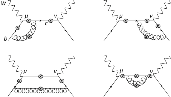
Figure 1: One-loop diagrams contributing to the current correlator. The background gluon can be attached wherever a cross is marked.

The calculation consists in matching the one-loop diagrams in Fig. 1, representing the correlator of two axial-vector currents computed in an expansion around the mass-shell of the $b$ quark, onto local HQET operators.

A recent independent calculation [45] of the semileptonic width at $m_{c}=0$ seems to be in agreement with the $m_{c}\to 0$ limit of [44]. Refs. [41, 44] provide analytic results for the $O(\alpha_{s}\Lambda_{\rm QCD}^{2}/m_{b}^{2})$ corrections to the three relevant structure functions and hence to the triple differential semileptonic $B$ decay width. The most general moment have now been computed to this order and employed to improve the precision of the fits to $|V_{cb}|$ [12].

Numerically, using for the heavy quark on-shell masses the values $m_{b}=4.6$ GeV and $m_{c}=1.15$ GeV, the total semileptonic width reads

$$\Gamma_{B\to X_{c}\ell\nu}=\Gamma_{0}\left[\left(1-1.78\,\frac{\alpha_{s}}{\pi}\right)\left(1-\frac{\mu_{\pi}^{2}}{2m_{b}^{2}}\right)-\left(1.94+2.42\,\frac{\alpha_{s}}{\pi}\right)\frac{\mu_{G}^{2}(m_{b})}{m_{b}^{2}}\right],$$

where $\Gamma_{0}$ is the tree level width and we have omitted higher order terms of $O(\alpha_{s}^{2})$ and $O(1/m_{b}^{3})$. The coefficient of $\mu_{\pi}^{2}$ is fixed by RI (or equivalently, by Lorentz invariance) at all orders. The parameter $\mu_{G}^{2}$ is renormalized at the scale $m_{b}$. It is advisable to evaluate the QCD coupling constant at a scale lower than $m_{b}$. If we adopt $\alpha_{s}=0.25$ the $O(\alpha_{s})$ correction increases the $\mu_{G}^{2}$ coefficient by about 7%. In the kinetic scheme with cutoff $\mu=1$GeV and for the same values of the masses the width becomes

$$\Gamma_{B\to X_{c}\ell\nu}=\Gamma_{0}\left[1-0.96\,\frac{\alpha_{s}}{\pi}-\left(\frac{1}{2}-0.99\,\frac{\alpha_{s}}{\pi}\right)\frac{\mu_{\pi}^{2}}{m_{b}^{2}}-\left(1.94+3.46\,\frac{\alpha_{s}}{\pi}\right)\frac{\mu_{G}^{2}(m_{b})}{m_{b}^{2}}\right],$$

where the NLO corrections to the coefficients of $\mu_{\pi}^{2},\mu_{G}^{2}$ are both close to 15% but have different signs. Overall, the $O(\alpha_{s}\Lambda^{2}_{\rm QCD}/m_{b}^{2})$ contributions decrease the total width by about 0.3%. However, NLO corrections also modify the coefficients of $\mu_{\pi}^{2},\mu_{G}^{2}$ in the moments which are fitted to extract the non-perturbative parameters, and will ultimately shift the values of the OPE parameters to be employed in the width. Therefore, in order to quantify the eventual numerical impact of the new corrections on the semileptonic width and on $|V_{cb}|$, a new global fit has to be performed.

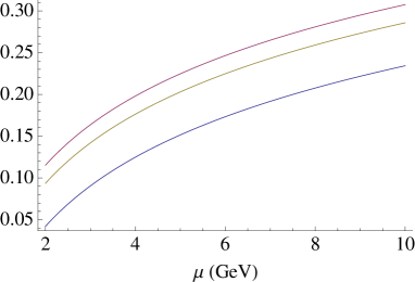
Figure 2: Relative NLO correction to the $\mu_{G}^{2}$ coefficients in the width (blue), first (red) and second central (yellow) leptonic moments as a function of the renormalization scale of $\mu_{G}^{2}$.

The size of the $O(\alpha_{s}\mu_{G}^{2}/m_{b}^{2})$ corrections depends on the renormalization scale $\mu$ of the chromomagnetic operator. This is illustrated in Fig. 2, where the size of the NLO correction relative to the tree level results is shown for the width and the first two leptonic central moments at different values of $\mu$. The NLO corrections are quite small for $\mu\approx 2$GeV and, as expected, increase with $\mu$. For $\mu\mathop{\mbox{\vbox{\hbox{$>$} \vskip-9.0pt\hbox{$\sim$} \vskip-3.0pt}}}m_{b}$ the running of $\mu_{G}^{2}$ appears to dominate the NLO corrections. In view of the importance of $O(1/m_{b}^{3})$ corrections, if a theoretical precision of 1% in the decay rate is to be reached, the $O(\alpha_{s}/m_{b}^{3})$ effects need to be calculated.

As to the higher power corrections, the $O(1/m_{b}^{4})$ and $O(1/m_{Q}^{5})$ effects were computed in [46]. The main problem here is the proliferation of non-perturbative parameters: as many as nine new expectation values appear at $O(1/m_{b}^{4})$ and more at the next order. Because they cannot all be extracted from experiment, in [46] they have been estimated in the ground state saturation approximation, thus reducing them to products of the known $O(1/m_{b}^{2,3})$ parameters, see also [47]. In this approximation, the total $O(1/m_{Q}^{4,5})$ correction to the width is about +1.3%. The $O(1/m_{Q}^{5})$ effects are dominated by $O(1/m_{b}^{3}m_{c}^{2})$ intrinsic charm contributions, amounting to +0.7% [20]. The net effect on $\it{|V_{cb}|}$ also depends on the corrections to the moments. Ref. [46] estimate that the overall effect on $\it{|V_{cb}|}$ is a 0.4% increase. While this sets the scale of higher order power corrections, it is as yet unclear how much the result depends on the assumptions made for the expectation values. A new preliminary global fit [48] performed using different ansatz for the new non-perturbative parameters seems to confirm that these corrections lead to a small shift in $\it{|V_{cb}|}$.

Two implementations of the OPE calculation have been employed in global analyses; they are based either on the kinetic scheme [21, 22, 39, 3] or on the $1S$ mass scheme for the $b$ quark mass [49, 50]. They both include power corrections up to and including $O(1/m_{b}^{3})$ and perturbative corrections of $O(\alpha_{s}^{2}\beta_{0})$. Beside differing in the perturbative scheme adopted, the global fits may include a different choice of experimental data, employ specific assumptions, or estimate the theoretical uncertainties in different ways. Recently, the kinetic scheme implementation has been upgraded to include first the complete $O(\alpha_{s}^{2})$ [38] and later the $(\alpha_{s}\Lambda^{2}/m_{b}^{2})$ [12] contributions.

4 $|V_{cb}|$ and the fit to semileptonic moments

The OPE parameters can be constrained by various moments of the lepton energy and hadron mass distributions of $B\to X_{c}\ell\nu$ that have been measured with good accuracy at the $B$-factories, as well as at CLEO, DELPHI, CDF [51, 6, 52, 53, 54, 55, 56]. The total semileptonic width can then be employed to extract $|V_{cb}|$. The situation is less favorable in the case of $|V_{ub}|$, where the total rate is much more difficult to access experimentally because of the background from $B\to X_{c}\ell\nu$, but the results of the semileptonic fits are crucial also in that case. This strategy has been rather successful and has allowed for a $\sim 2\%$ determination of $V_{cb}$ and for a $\sim 5\%$ determination of $V_{ub}$ from inclusive decays [14, 82].

The first few moments of the charged lepton energy spectrum in $B\to X_{c}\ell\nu$ decays are experimentally measured with high precision — better than 0.2% in the case of the first moment. At the $B$-factories a lower cut on the lepton energy, $E_{\ell}\geq E_{cut}$, is applied to suppress the background. Experiments measure the moments at different values of $E_{cut}$, which provides additional information as the cut dependence is also a function of the OPE parameters. The relevant quantities are therefore $\ell_{1,2,3}$, $h_{1,2,3}$, as well as the ratio $R^{*}$ between the rate with and without a cut

$$R^{*}(E_{cut})=\frac{\int_{E_{cut}}^{E_{max}}dE_{\ell}\ \frac{d\Gamma}{dE_{\ell}}}{\int_{0}^{E_{max}}dE_{\ell}\ \frac{d\Gamma}{dE_{\ell}}}\ .$$ (9)

This quantity is needed to relate the actual measurement of the rate with a cut to the total rate, from which one conventionally extracts $|V_{cb}|$. All of these observables can be expressed as double expansions in $\alpha_{s}$ and inverse powers of $m_{b}$, schematically

$$M_{i} = M_{i}^{(0)}+\frac{\alpha_{s}(\mu)}{\pi}M_{i}^{(1)}+\left(\frac{\alpha_{s}}{\pi}\right)^{2}M_{i}^{(2)}+\left(M_{i}^{(\pi,0)}+\frac{\alpha_{s}(\mu)}{\pi}M_{i}^{(\pi,1)}\right)\frac{\mu_{\pi}^{2}}{m_{b}^{2}}$$ (10)

$$+\left(M_{i}^{(G,0)}+\frac{\alpha_{s}(\mu)}{\pi}M_{i}^{(G,1)}\right)\frac{\mu_{G}^{2}}{m_{b}^{2}}+M_{i}^{(D)}\frac{\rho_{D}^{3}}{m_{b}^{3}}+M_{i}^{(LS)}\frac{\rho_{LS}^{3}}{m_{b}^{3}}+\dots$$

where all the coefficients $M_{i}^{(j)}$ depend on $m_{c}$, $m_{b}$, $E_{cut}$, and on various renormalization scales. The dots represent missing terms of $O(\alpha_{s}^{3})$, $O(\alpha_{s}^{2}/m_{b}^{2})$, $O(\alpha_{s}/m_{b}^{3})$, and $O(1/m_{b}^{4})$, which are either unknown or not yet included in the latest analysis [12]. It is worth stressing that according to the adopted definition the OPE parameters $\mu_{\pi}^{2}$, … are matrix elements of local operators evaluated in the physical $B$ meson, i.e. without taking the infinite mass limit.

The semileptonic moments are sensitive to a specific linear combination of $m_{c}$ and $m_{b}$, $\approx m_{b}-0.8m_{c}$ [57], see Fig. 3, which is close to the one needed for the extraction of $\it{|V_{cb}|}$, but they cannot resolve the individual masses with good accuracy. It is important to check the consistency of the constraints on $m_{c}$ and $m_{b}$ from semileptonic moments with precise determinations of these quark masses, as a step in the effort to improve our theoretical description of inclusive semileptonic decays. Moreover, the inclusion of these constraints in the semileptonic fits improves the accuracy of the $\it{|V_{ub}|}$ and $\it{|V_{cb}|}$ determinations. The heavy quark masses and the non-perturbative parameters obtained from the fits are also relevant for a precise calculation of other inclusive decay rates such as that of $B\to X_{s}\gamma$ [58].

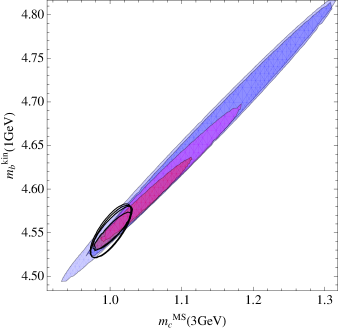
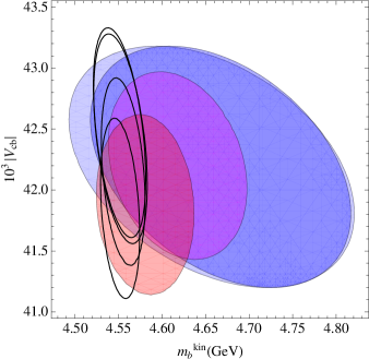
Figure 3: Two-dimensional projections of the fits performed with different assumptions for the theoretical correlations. The orange, magenta, blue, light blue 1-sigma regions correspond to the four scenarios considered in [58]. The black contours show the same regions when the $m_{c}$ constraint of Ref. [59] is employed.

In the past, the first two moments of the photon energy in $B\to X_{s}\gamma$ have generally been employed to improve the accuracy of the fit. Indeed, the first moment corresponds to a determination of $m_{b}$. However, in recent years rather precise determinations of the heavy quark masses ($e^{+}e^{-}$ sum rules, lattice QCD etc.) have become available, based on completely different methods, see e.g. [60, 59, 61, 62, 63, 64, 65, 66, 67, 68] and [69, 70] for reviews. The charm mass determinations have a smaller absolute uncertainty and appear quite consistent with each other, providing a good external constraint for the semileptonic fits. Radiative moments remain interesting in their own respect, but they are not competitive with the charm mass determinations. Moreover, experiments place a lower cut on the photon energy, which introduces a sensitivity to the Fermi motion of the $b$-quark inside the $B$ meson and tends to disrupt the OPE. One can still resum the higher-order terms into a non-local distribution function and parameterize it assuming different functional forms [71, 72, 73], but the parameterization will depend on $m_{b},\mu_{\pi}^{2}$ etc., namely the same parameters one wants to extract. Another serious problem is that only the leading operator contributing to inclusive radiative decays can be described by an OPE. Therefore, radiative moments are in principle subject to additional $O(\Lambda_{QCD}/m_{b})$ effects, which have not yet been estimated [74]. For all these reasons the most recent analyses [58, 12] have relied solely on charm and possibly bottom mass determinations.

The global fits of Refs. [58, 12] are performed in the kinetic scheme with a cutoff $\mu=1\,\mbox{GeV}$ and follow the implementation described in [3, 38]. The two fits only differ in the inclusion of $O(\alpha_{s}^{2}/m_{b}^{2})$ corrections and in the consequent reduction of theoretical uncertainties. In order to use the high precision $m_{c}$ determinations without introducing additional theoretical uncertainty due to the mass scheme conversion, it is convenient to employ the $\overline{\rm MS}$ scheme for the charm mass, denoted by $\overline{m}_{c}(\mu_{c})$, and to choose a normalization scale $\mu_{c}$ well above $m_{c}$, e.g. 3  GeV.

The experimental data for the moments are fitted to the theoretical expressions in order to constrain the non-perturbative parameters and the heavy quark masses. 43 measurements are included, see [58] for the list. The chromomagnetic expectation value $\mu_{G}^{2}$ is also constrained by the hyperfine splitting

$$M_{B^{*}}-M_{B}=\frac{2}{3}\frac{\mu_{G}^{2}}{m_{b}}+O\left(\frac{\alpha_{s}\mu_{G}^{2}}{m_{b}},\frac{1}{m_{b}^{2}}\right).$$

Unfortunately, little is known of the power corrections to the above relation and only a loose bound [75] can be set, see [11] for a recent discussion. For what concerns $\rho_{LS}^{3}$, it is somewhat constrained by the heavy quark sum rules [75]. Refs. [58, 12] use the constraints

$$\mu_{G}^{2}=(0.35\pm 0.07)\,\mbox{GeV}^{2},\qquad\rho_{LS}^{3}=(-0.15\pm 0.10)\,\mbox{GeV}^{3}\,.$$ (11)

It should be stressed that $\rho_{LS}^{3}$ plays a minor role in the fits because its coefficients are generally suppressed with respect to the other parameters.

It is interesting to note that the fit without theoretical uncertainties is not good, with $\chi^{2}/dof\sim 2$, corresponding to a very small $p$-value and driven by a strong tension ($\sim 3.5\sigma$) between the constraints in Eq. (11) and the measured moments. On the other hand, the fit without the constraints (11) is not too bad. Indeed, theoretical uncertainties are not so much necessary for the OPE expressions to fit the moments — that would merely test Eq.(10) as a parameterization; they are instead needed to preserve the definition of the parameters as $B$ expectation values of certain local operators, which in turn can be employed in the semileptonic widths and in other applications of the Heavy Quark Expansion.

As noted above, the OPE description of semileptonic moments is subject to two sources of theoretical uncertainty: missing higher order terms in Eq. (10) and terms that violate quark-hadron duality. Only of the first kind of uncertainty is usually considered: the violation of local quark-hadron duality would manifest itself as an inconsistency of the fit, which as we will see is certainly not present at the current level of theoretical and experimental accuracy.

In [12] we assume that missing perturbative corrections can affect the coefficients of $\mu_{\pi}^{2}$ and $\mu_{G}^{2}$ at the level of $\pm 7\%$, while missing perturbative and higher power corrections can effectively change the coefficients of $\rho_{D}^{3}$ and $\rho_{LS}^{3}$ by $\pm 30\%$. Moreover we assign an irreducible theoretical uncertainty of 8 MeV to the heavy quark masses, and vary $\alpha_{s}(m_{b})$ by 0.018. The changes in $M_{i}$ due to these variations of the fundamental parameters are added in quadrature and provide a theoretical uncertainty $\delta M_{i}^{th}$, to be subsequently added in quadrature with the experimental one, $\delta M_{i}^{exp}$. This method is consistent with the residual scale dependence observed at NNLO, and appears to be reliable: the NNLO corrections and the $O(1/m_{b}^{4,5})$ (using ground state saturation as in [46]) have been found to be within the range of expectations based on the method in the original formulation of [3].

The correlation between theoretical errors assigned to different observables is much harder to estimate, but plays an important role in the semileptonic fits. Let us first consider moments computed at a fixed value of $E_{cut}$: as long as one deals with central higher moments, there is no argument of principle supporting a correlation between two different moments, for instance $\ell_{1}$ and $h_{2}$. We also do not observe any clear pattern in the known corrections, and therefore regard the theoretical predictions for different central moments as completely uncorrelated. Let us now consider the calculation of a certain moment $M_{i}$ for two close values of $E_{cut}$, say 1 GeV and 1.1 GeV. Clearly, the OPE expansion for $M_{i}(1\,\mbox{GeV})$ will be very similar to the one for $M_{i}(1.1\,\mbox{GeV})$, and we may expect this to be true at any order in $\alpha_{s}$ and $1/m_{b}$. The theoretical uncertainties we assign to $M_{i}(1\,\mbox{GeV})$ and $M_{i}(1.1\,\mbox{GeV})$ will therefore be very close to each other and very highly correlated. The degree of correlation between the theory uncertainty of $M_{i}(E_{1})$ and $M_{i}(E_{2})$ can intuitively be expected to decrease as $|E_{1}-E_{2}|$ grows. Moreover, we know that higher power corrections are going to modify significantly the spectrum only close to the endpoint. Indeed, one observes that the $O(1/m_{b}^{4,5})$ contributions are equal for all cuts below about 1.2 GeV (see Fig.2 of [46]) and the same happens for the $O(\alpha_{s}\mu_{\pi}^{2}/m_{b}^{2})$ corrections [40]. Therefore, the dominant sources of current theoretical uncertainty suggest very high correlations among the theoretical predictions of the moments for cuts below roughly 1.2  GeV.

Various assumptions on the theoretical correlations have been tried. A 100% correlation between a certain central moment computed at different values of $E_{cut}$ has been assumed e.g. in [7]). This is too strong an assumption, which ends up distorting the fit because the dependence of $M_{i}$ on $E_{cut}$, itself a function of the fit parameters, is then free of theoretical uncertainty. A fit performed in this way will underestimate the uncertainties. Another possibility has been proposed in Ref. [50], with the theoretical correlation matrix equal to the experimental one.

Four alternative approaches for the theoretical correlations are compared in [58]. Fig. 3 shows some of the results of the fits performed with the four options for the theoretical correlations. The fits include the two constraints of Eq. (11). In general, the results depend sensitively on the option adopted. In the case of the heavy quark masses, which are strongly correlated, we observe large errors differing significantly between the various options, although the central values are quite consistent. The results for the non-perturbative parameters depend even stronger on the option. The inclusion of precise mass constraints in the fit decreases the errors and neutralizes the ambiguity due to the ansatz for the theoretical correlations. It also allows us to check the consistency of the results with independent information. The effect of the inclusion of a precise charm mass constraint in the semileptonic fit is illustrated in Fig. 3. As expected, the uncertainty in the $b$ mass becomes about 20-25MeV in all scenarios, a marked improvement, also with respect to the precision resulting from the use of radiative moments [14]. The inclusion of the $m_{c}$ constraint indeed stabilized the fits with respect to the ansatz for the theory correlations. On the other hand, there is hardly any improvement in the final precision of the non-perturbative parameters and of $|V_{cb}|$.

Figs. 4 show two examples of leptonic and hadronic moments measurements compared with their theoretical prediction based on the results of the fit of [58] with theory uncertainty. As anticipated, theory errors are generally larger than experimental ones. The situation is similar also for the fits in [12].

The default fit of [12] uses $\overline{m}_{c}(3\,\mbox{GeV})=0.986(13)$ GeV [60]; the results are shown in Table 4,

Results of the global fit with $m_{c}$ constraint in the default scenario of [12]. All parameters are in  GeV at the appropriate power and all, except $m_{c}$, in the kinetic scheme at $\mu=1\,\mbox{GeV}$. The last row gives the uncertainties. $m_{b}^{kin}$ $\overline{m_{c}}(3\,\mbox{GeV})$ $\mu_{\pi}^{2}$ $\rho_{D}^{3}$ $\mu_{G}^{2}$ $\rho_{LS}^{3}$ ${\rm BR}_{c\ell\nu}$ (%) $10^{3}\,|V_{cb}|$ 4.553 0.987 0.465 0.170 0.332 -0.150 10.65 42.21 0.020 0.013 0.068 0.038 0.062 0.096  0.16  0.78

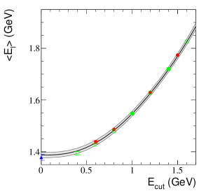
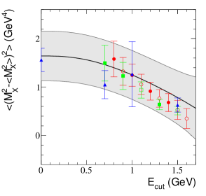
Figure 4: Default fit predictions for $\ell_{1}$ and $h_{2}$ compared with measured values as functions of $E_{cut}$. The grey band is the theory prediction with total theory error. Filled symbols mean that the point was used in the fit. Open symbols are measurements that were not used in the fit. BaBar data are shown by circles, Belle by squares and other experiments (DELPHI, CDF, CLEO) by triangles.

where the bottom mass is expressed in the kinetic scheme, $m_{b}^{kin}(1\,\mbox{GeV})$. Most available $m_{b}$ determinations, however, use the $\overline{\rm MS}$ mass $\overline{m}_{b}(\overline{m}_{b})$ which is not well-suited to the description of semileptonic $B$ decays as the calculation of the width and moments in terms of $\overline{m}_{b}(\overline{m}_{b})$ involves large higher order corrections. Since the relation between the kinetic and the $\overline{\rm MS}$ masses is known only to $O(\alpha_{s}^{2})$, the ensuing uncertainty is not negligible. It has been estimated to be about 30 MeV [38],

$$m_{b}^{kin}(1\,\mbox{GeV})-\overline{m}_{b}(\overline{m}_{b})=0.37\pm 0.03\,\mbox{GeV},$$

leading to a preferred value

$$\overline{m}_{b}(\overline{m}_{b})=4.183\pm 0.037\,\mbox{GeV},$$

in good agreement with various recent $m_{b}$ determinations [60, 76, 77, 78, 79, 80, 81, 68], as illustrated in Fig.5. Of course, one can also include in the fit both $m_{c}$ and $m_{b}$ determinations, but because of the scheme translation error in $m_{b}$ the gain in accuracy is limited [58, 12].

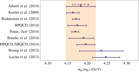
Figure 5: Comparison of different $\overline{m}_{b}(\overline{m}_{b})$ determinations [12, 60, 76, 77, 78, 79, 80, 81, 68]. The dashed line denotes the error before scheme conversion.

As already noted, the semileptonic moments are highly sensitive to a linear combination of the heavy quark masses. When no external constraint is imposed on $m_{c,b}$, the semileptonic moments determine best a linear combination of the heavy quark masses which is close to their difference,

$$m_{b}^{kin}(1\,\mbox{GeV})-0.85\,\overline{m}_{c}(3\,\mbox{GeV})=3.714\pm 0.018\,\mbox{GeV},.$$ (12)

The value of $|V_{cb}|$ is computed using

$$|V_{cb}|=\sqrt{\frac{|V_{cb}|^{2}\,{\rm BR}_{c\ell\nu}}{\tau_{B}\,\Gamma_{B\to X_{c}\ell\nu}^{OPE}},}$$ (13)

with $\tau_{B}=1.579(5)$ps [14]. Its theoretical error is computed combining in quadrature the parametric uncertainty that results from the fit, and an additional 1.3% theoretical error to take into account missing higher order corrections in the expression for the semileptonic width. It turns out that using $\overline{m}_{c}(2\,\mbox{GeV})$ rather than $\overline{m}_{c}(2\,\mbox{GeV})$ leads to a better converging expansion for the width, with smaller theoretical error for $|V_{cb}|$, about 1%. However, the value of $|V_{cb}|$ extracted in this way, $42.01(68)\times 10^{-3}$ is compatible with that in Table 1. The same holds if the kinetic scheme is used also for $m_{c}$, in which case we obtain $|V_{cb}|=42.04(67)\times 10^{-3}$.

The fits are generally good, with $\chi^{2}/d.o.f.\approx 0.4$ for the default fit. The low $\chi^{2}$ of the default fit is due to the large theoretical uncertainties we have assumed. It may be tempting to interpret it as evidence that the theoretical errors have been overestimated. However, higher order corrections may effectively shift the parameters of the $O(1/m_{b}^{2})$ and $O(1/m_{b}^{3})$ contributions. If we want to maintain the formal definition of these parameters, and to be able to use them elsewhere, we therefore have to take into account the potential shift they may experience because of higher order effects.

The fits with a constraint on $m_{c}$ are quite stable with respect to a change of inputs. In particular, small differences are found when experimental data at high $E_{cut}$ are excluded, and when only hadronic or leptonic moments are considered. One may also wonder whether the inclusion of moments measured at different values of $E_{cut}$ really benefits the final accuracy. It turns out that the benefit is minor but non-negligible.

In the kinetic scheme the inequalities $\mu_{\pi}^{2}(\mu)\!\geq\!\mu_{G}^{2}(\mu)$, $\rho_{D}^{3}(\mu)\!\geq\!-\rho_{LS}^{3}(\mu)$ hold at arbitrary values of the cutoff $\mu$. The central values of the fit satisfy the inequalities. The dependence of the results on the scales of $\alpha_{s}$ and on the kinetic cutoff has been studied in [12]. Changing the scale of $\alpha_{s}$ from $m_{b}$ to 2 GeV the value of $|V_{cb}|$ increases by only 0.5%, well within its error, while $m_{b}$ increases by less than 0.4%.

5 Conclusions

We have seen that the most recent value of $|V_{cb}|$ extracted from an analysis of inclusive semileptonic $B$ decays is [12]

$$|V_{cb}|=(42.21\pm 0.78)\times 10^{-3}.$$ (14)

A competitive determination of $|V_{cb}|$ derives from a comparison of the extrapolation of the $B\to D^{*}l\nu$ rate to the zero-recoil point with an unquenched lattice QCD calculation of the zero recoil form factor by the Fermilab-MILC collaboration [13],

$$|V_{cb}|=(39.04\pm 0.49_{exp}\pm 0.53_{lat}\pm 0.19_{QED})\times 10^{-3},$$ (15)

where the error is split into experimental, lattice and QED components. The values in Eqs. (14,15) disagree by $2.9\sigma$. This is a long-standing tension, which has become stronger with recent improvements in the OPE and lattice calculations. A few comments are in order:

• The zero-recoil form factor of $B\to D^{*}l\nu$ can also be estimated using heavy quark sum rules, see [10, 11] for a recent reanalysis. Although this method is subject to larger uncertainties and it is difficult to improve its accuracy, it leads to a $|V_{cb}|$ compatible with the inclusive determination, $|V_{cb}|=40.93(1.11)\times 10^{-3}$. There exist also less precise determinations of $|V_{cb}|$ based on the decay $B\to Dl\nu$, but they do not help resolving the issue at the moment, see [82] for a review.

• The extrapolation of the $B\to D^{*}l\nu$ experimental data to the zero-recoil point is performed by the experimental collaborations using the Caprini-Lellouch-Neubert parameterization [83], based on HQET at next-to-leading order and expected to reproduce the form factor within 2% (not included in the present error budget). While this rigid parameterization with only two free parameters fits well the experimental data at $w\neq 1$, at the present level of precision its use to extrapolate the rate to zero recoil is questionable. Lattice calculations of the form factors at non-zero recoil are currently under way; they would allow us to avoid the extrapolation.

• It is also possible to determine $|V_{cb}|$ indirectly, using the CKM unitarity relations together with CP violation and flavor data, without the above direct information: SM analyses of this kind by the UTfit and CKMFitter collaborations give $(42.05\pm 0.65)\times 10^{-3}$ [84] and $(41.4^{+2.4}_{-1.4})\times 10^{-3}$ [85], both closer to the inclusive value of Eq. (14).

In principle, the discrepancy between the values of $|V_{cb}|$ extracted from inclusive decays and from $B\to D^{*}l\nu$ could be ascribed to physics beyond the SM, as the $B\to D^{*}$ transition is sensitive only to the axial-vector component of the $V-A$ charged weak current. However, the new physics effect should be sizable (8%), and it would require new interactions which seem ruled out by electroweak constraints on the effective $Zb\bar{b}$ vertex [86]. The most likely explanation of the discrepancy between Eqs. (14,15) is therefore a problem in the theoretical and/or experimental analyses of semileptonic decays.

I do not have space here to discuss the closely related determination of $|V_{ub}|$ from inclusive semileptonic $B$ decays without charm, which shows a similar puzzling tension between inclusive and exclusive determinations. However, I cannot avoid stressing the central role played by Kolya from the beginning also in this field [72, 87, 88, 9]. The interested reader is referred to [82] for a recent review.

This work is supported in part by MIUR under contract 2010YJ2NYW 006, by the EU Commission through the HiggsTools Initial Training Network PITN-GA-2012-316704, and by Compagnia di San Paolo under contract ORTO11TPXK.

References

- [1] M. Battaglia et al., Phys. Lett. B556, 41–49, (2003). arXiv:hep-ph/0210319.
- [2] N. Uraltsev, Nucl. Phys. Proc. Suppl. 117, pp. 554–557, (2002). arXiv:hep-ph/0210044.
- [3] P. Gambino and N. Uraltsev, Eur.Phys.J. C34, 181–189, (2004). arXiv:hep-ph/0401063.
- [4] A. Mahmood et al., Phys.Rev. D70, 032003, (2004). arXiv:hep-ex/0403053.
- [5] B. Aubert et al., Phys. Rev. D69, 111103, (2004). arXiv:hep-ex/0403031.
- [6] B. Aubert et al., Phys. Rev. Lett. 93, 011803, (2004). arXiv:hep-ex/0404017.
- [7] O. Büchmuller and H. Flächer, Phys. Rev. D73, 073008, (2006). arXiv:hep-ph/0507253.
- [8] V. Aquila, P. Gambino, G. Ridolfi, and N. Uraltsev, Nucl.Phys. B719, 77–102, (2005). arXiv:hep-ph/0503083.
- [9] P. Gambino, P. Giordano, G. Ossola, and N. Uraltsev, JHEP. 0710, 058, (2007). arXiv:0707.2493.
- [10] P. Gambino, T. Mannel, and N. Uraltsev, Phys.Rev. D81, 113002, (2010). arXiv:1004.2859.
- [11] P. Gambino, T. Mannel, and N. Uraltsev, JHEP. 1210, 169, (2012). arXiv:1206.2296.
- [12] A. Alberti, P. Gambino, K. J. Healey, and S. Nandi. (2014). arXiv:1411.6560.
- [13] J. A. Bailey, et al. (2014). arXiv:1403.0635.
- [14] Y. Amhis et al. (2012). arXiv:1207.1158.
- [15] J. Chay, H. Georgi and B. Grinstein, Phys.Lett. B247 399 (1990).
- [16] I. I. Bigi, N. Uraltsev, and A. Vainshtein, Phys.Lett. B293, 430–436, (1992). arXiv:hep-ph/9207214.
- [17] I. I. Bigi, M. A. Shifman, N. Uraltsev, and A. I. Vainshtein, Phys.Rev.Lett. 71, 496–499, (1993). arXiv:hep-ph/9304225.
- [18] B. Blok, L. Koyrakh, M. A. Shifman, and A. Vainshtein, Phys.Rev. D49, 3356, (1994). arXiv:hep-ph/9307247.
- [19] A. V. Manohar and M. B. Wise, Phys.Rev. D49, 1310–1329, (1994). arXiv:hep-ph/9308246.
- [20] I. Bigi, T. Mannel, S. Turczyk, and N. Uraltsev, JHEP. 1004, 073, (2010). arXiv:0911.3322.
- [21] I. I. Bigi et al., Phys.Rev. D56, 4017–4030, (1997). arXiv:hep-ph/9704245.
- [22] I. I. Bigi et al., Phys.Rev. D52, 196–235, (1995). arXiv:hep-ph/9405410.
- [23] M. Gremm and A. Kapustin, Phys.Rev. D55, 6924–6932, (1997). arXiv:hep-ph/9603448.
- [24] I. I. Bigi and N. Uraltsev, Int.J.Mod.Phys. A16, 5201–5248, (2001). arXiv:hep-ph/0106346.
- [25] M. Jezabek and J. H. Kuhn, Nucl.Phys. B314, 1, (1989).
- [26] M. Jezabek and J. H. Kuhn, Nucl.Phys. B320, 20, (1989).
- [27] A. Czarnecki and M. Jezabek, Nucl.Phys. B427, 3–21, (1994). arXiv:hep-ph/9402326.
- [28] M. Gremm and I. W. Stewart, Phys.Rev. D55, 1226–1232, (1997). arXiv:hep-ph/9609341.
- [29] S. J. Brodsky, G. P. Lepage, and P. B. Mackenzie, Phys.Rev. D28, 228, (1983).
- [30] A. Czarnecki, M. Jezabek, and J. H. Kuhn, Acta Phys.Polon. B20, 961, (1989).
- [31] A. F. Falk, M. E. Luke, and M. J. Savage, Phys.Rev. D53, 2491–2505, (1996). arXiv:hep-ph/9507284.
- [32] A. F. Falk and M. E. Luke, Phys.Rev. D57, 424–430, (1998). arXiv:hep-ph/9708327.
- [33] M. Trott, Phys.Rev. D70, 073003, (2004). arXiv:hep-ph/0402120.
- [34] N. Uraltsev, Int.J.Mod.Phys. A20, 2099–2118, (2005). arXiv:hep-ph/0403166.
- [35] A. Pak and A. Czarnecki, Phys.Rev.Lett. 100, 241807, (2008). arXiv:0803.0960.
- [36] K. Melnikov, Phys.Lett. B666, 336–339, (2008). arXiv:0803.0951.
- [37] S. Biswas and K. Melnikov, JHEP. 1002, 089, (2010). arXiv:0911.4142.
- [38] P. Gambino, JHEP. 1109, 055, (2011). arXiv:1107.3100.
- [39] D. Benson, I. Bigi, T. Mannel, and N. Uraltsev, Nucl.Phys. B665, 367–401, (2003). arXiv:hep-ph/0302262.
- [40] T. Becher, H. Boos, and E. Lunghi, JHEP. 0712, 062, (2007). arXiv:0708.0855.
- [41] A. Alberti, T. Ewerth, P. Gambino, and S. Nandi, Nucl.Phys. B870, 16–29, (2013). arXiv:1212.5082.
- [42] M. E. Luke and A. V. Manohar, Phys.Lett. B286, 348–354, (1992). arXiv:hep-ph/9205228.
- [43] A. V. Manohar, Phys.Rev. D82, 014009, (2010). arXiv:1005.1952.
- [44] A. Alberti, P. Gambino, and S. Nandi, JHEP. 1401, 1–16, (2014). arXiv:1311.7381.
- [45] T. Mannel, A. A. Pivovarov, and D. Rosenthal. (2014). arXiv:1405.5072.
- [46] T. Mannel, S. Turczyk, and N. Uraltsev, JHEP. 1011, 109, (2010). arXiv:1009.4622.
- [47] J. Heinonen and T. Mannel, Nucl.Phys. B889, 46–63, (2014). arXiv:1407.4384.
- [48] P. Gambino and S. Turzcyk, work in progress.
- [49] A. H. Hoang, Z. Ligeti, and A. V. Manohar, Phys.Rev. D59, 074017, (1999). arXiv:hep-ph/9811239.
- [50] C. W. Bauer, Z. Ligeti, M. Luke, A. V. Manohar, and M. Trott, Phys.Rev. D70, 094017, (2004). arXiv:hep-ph/0408002.
- [51] S. Csorna et al., Phys.Rev. D70, 032002, (2004). arXiv:hep-ex/0403052.
- [52] B. Aubert et al., Phys.Rev. D81, 032003, (2010). arXiv:0908.0415.
- [53] P. Urquijo et al., Phys.Rev. D75, 032001, (2007). arXiv:hep-ex/0610012.
- [54] C. Schwanda et al., Phys.Rev. D75, 032005, (2007). arXiv:hep-ex/0611044.
- [55] D. Acosta et al., Phys.Rev. D71, 051103, (2005). arXiv:hep-ex/0502003.
- [56] J. Abdallah et al., Eur.Phys.J. C45, 35–59, (2006). arXiv:hep-ex/0510024.
- [57] M. Voloshin, Phys.Rev. D51, 4934–4938, (1995). arXiv:hep-ph/9411296.
- [58] P. Gambino and C. Schwanda, Phys.Rev. D89, 014022, (2014). arXiv:1307.4551.
- [59] B. Dehnadi, A. H. Hoang, V. Mateu, and S. M. Zebarjad, JHEP. 1309, 103, (2013). arXiv:1102.2264.
- [60] K. G. Chetyrkin et al., Phys. Rev. D80, 074010, (2009). arXiv:0907.2110.
- [61] S. Bodenstein et al., Phys. Rev. D83, 074014, (2011). arXiv:1102.3835.
- [62] A. Signer, Phys. Lett. B672, 333–338, (2009). arXiv:0810.1152.
- [63] I. Allison et al., Phys. Rev. D78, 054513, (2008). arXiv:0805.2999.
- [64] C. McNeile et al., Phys. Rev. D82, 034512, (2010). arXiv:1004.4285.
- [65] B. Blossier et al., Phys. Rev. D82, 114513, (2010). arXiv:1010.3659.
- [66] J. Heitger, G. M. von Hippel, S. Schaefer, and F. Virotta, PoS. LATTICE2013, 475, (2013). arXiv:1312.7693.
- [67] N. Carrasco et al., Nucl.Phys. B887, 19–68, (2014). arXiv:1403.4504.
- [68] W. Lucha, D. Melikhov, and S. Simula, Phys.Rev. D88(5), 056011, (2013). arXiv:1305.7099.
- [69] M. Antonelli et al., Phys.Rept. 494, 197–414, (2010). arXiv:0907.5386.
- [70] J. Beringer et al., Phys.Rev. D86, 010001, (2012).
- [71] M. Neubert, Phys.Rev. D49, 4623–4633, (1994). arXiv:hep-ph/9312311.
- [72] I. I. Bigi, M. A. Shifman, N. Uraltsev, and A. Vainshtein, Int.J.Mod.Phys. A9, 2467–2504, (1994). arXiv:hep-ph/9312359.
- [73] D. Benson, I. Bigi, and N. Uraltsev, Nucl.Phys. B710, 371–401, (2005). arXiv:hep-ph/0410080.
- [74] G. Paz. (2010). arXiv:1011.4953.
- [75] N. Uraltsev, Phys.Lett. B545, 337–344, (2002). arXiv:hep-ph/0111166.
- [76] S. Bodenstein et al., Phys.Rev. D85, 034003, (2012). arXiv:1111.5742.
- [77] M. Beneke et al. arXiv:1411.3132.
- [78] B. Colquhoun et al. arXiv:1408.5768.
- [79] B. Chakraborty et al. (2014). arXiv:1408.4169.
- [80] A. Hoang, P. Ruiz-Femenia, and M. Stahlhofen, JHEP. 1210, 188, (2012). arXiv:1209.0450.
- [81] A. A. Penin and N. Zerf, JHEP. 1404, 120, (2014). arXiv:1401.7035.
- [82] A. Bevan et al., Eur.Phys.J. C74(11), 3026, (2014). arXiv:1406.6311.
- [83] I. Caprini, L. Lellouch, and M. Neubert, Nucl.Phys. B530, 153–181, (1998). arXiv:hep-ph/9712417.
- [84] M. Bona et al., JHEP. 0610, 081, (2006). arXiv:hep-ph/0606167, see http://www.utfit.org for the latest results.
- [85] J. Charles et al., Eur.Phys.J. C41, 1–131, (2005). arXiv:hep-ph/0406184, see http://ckmfitter.in2p3.fr for recent results.
- [86] A. Crivellin and S. Pokorski. (2014). arXiv:1407.1320.
- [87] I. I. Bigi, R. Dikeman, and N. Uraltsev, Eur.Phys.J. C4, 453–461, (1998). arXiv:hep-ph/9706520.
- [88] N. Uraltsev, Int.J.Mod.Phys. A14, 4641–4652, (1999). arXiv:hep-ph/9905520.