Abstract

We present a class of linear programming approximations for mixed-integer polynomial optimization problems that take advantage of structured sparsity of the constraint matrix. In particular, we show that if the intersection graph of the constraints has tree-width bounded by a constant, then for any desired tolerance there is a linear programming formulation of polynomial size. Via an additional reduction, we obtain a polynomial-time approximation scheme for the “AC-OPF” problem on graphs with bounded tree-width. These constructions partly rely on a general construction for pure binary optimization problems where individual constraints are available through a membership oracle; if the intersection graph for the constraints has bounded tree-width our construction is of linear size and exact. This improves on a number of results in the literature, both from the perspective of formulation size and generality.

1 Introduction

A fundamental paradigm in the solution of integer programming and combinatorial optimization problems is the use of extended, or lifted, formulations, which rely on the binary nature of the variables and on the structure of the constraints to generate higher-dimensional convex relaxations with provably strong attributes. In this paper we consider mixed-integer polynomial optimization problems. We develop a reformulation operator which relies on the combinatorial structure of the constraints to produce linear programming approximations which attain provable bounds. A major focus is on polynomial optimization problems over networks and our main result in this context (Theorem 7 below) implies as a corollary that there exist polynomial-size linear programs that approximate the AC-OPF problem and the fixed-charge network flow problem on bounded tree-width graphs.

Our work relies on the concepts of intersection graph and tree-width; as has been observed before ([12], [39], [35], [56], [54]), the combination of these two concepts makes it possible to define a notion of structured sparsity in an optimization context that we will exploit here (see below for more references). The intersection graph of a system of constraints is a central concept originally introduced in [24] and which has been used by many authors, sometimes using different terminology.

Definition 1

The intersection graph of a system of constraints is the undirected graph which has a vertex for each variable and an edge for each pair of variables that appear in any common constraint.

Example 2

Consider the system of constraints on variables $x_{1},x_{2},x_{3}$ and $x_{4}$.

$$\begin{array}[]{lll}(1)\ 3x_{1}^{2}-\log_{2}(1+x_{2})\geq 0,&(2)\ -2x_{2}^{2}\ +\ (1+x_{3})^{3}\ \geq\ 0,&(3)\ x_{3}x_{5}=0\\ (5)\ x_{3}^{3}\ -\ 2-x_{4}^{2}\ <\ 0,&(5)\ (x_{1},x_{4})\in A&\end{array}$$ (1)

Where $A$ is some arbitrary set. Then the intersection graph has vertices $\{1,2,3,4,5\}$ and edges $\{1,2\}$, $\{2,3\}$, $\{3,4\}$, $\{3,5\}$ and $\{4,1\}$.

Definition 3

An undirected graph has tree-width $\leq k$ if it is contained in a chordal graph with clique number $\leq k+1$.

The tree-width concept was explicitly defined in [48] (also see [49]), but there are many equivalent definitions. An earlier discussion is found in [30] and closely related concepts have been used by many authors under other names, e.g. the “running intersection” property, and the notion of “partial k-trees”. An important known fact is that an $n$-vertex graph with tree-width $\leq k$ has $O(k^{2}n)$ edges, and thus low tree-width graphs are sparse, although the converse is not true. In the context of this paper, we can exploit structural sparsity in an optimization problem when the tree-width of the intersection graph is small. We also note that bounded tree-width can be recognized in linear time [15].

Our focus, throughout, is on obtaining polynomial-size LP formulations. The construction of such “compact” formulations is a goal of fundamental theoretical importance and quite separate from the development of polynomial-time algorithms. From a numerical perspective, additionally, the representation of a problem as an LP permits the use of practical bounding techniques such as cutting-plane and column-generation algorithms. We first prove:

Theorem 4

Consider a mixed-integer, linear objective, polynomially constrained problem

(PO): $$\min~{}c^{T}x$$ (2a)

subject to: $$\quad\quad f_{i}(x)\ \geq\ 0\quad 1\leq i\leq m$$ (2c)

$$\quad\quad x_{j}\in\{0,1\}\quad 1\leq j\leq p,\quad x_{j}\in[0,1]\quad p+1\leq j\leq n.$$

Let $\pi$ and $F$ be such that for $0\leq i\leq m$, $f_{i}(x)$ has maximum degree at most $\pi$ and $L_{1}$-norm of coefficients at most $F$. If the intersection graph of the constraints has tree-width $\leq\omega$ then for any $0<\epsilon<1$, there is a linear programming formulation with $O\left((2\pi/\epsilon)^{\omega+1}\,n\log(\pi/\epsilon)\right)$ variables and constraints that solves $\mathcal{P}$ within feasibility tolerance $F\epsilon$ and optimality tolerance $\|c\|_{1}\epsilon$.

Below we will provide an extended statement for this result, as well as a precise definition of ‘tolerance’. However, the statement in Theorem 4 is indicative of the fact that as $\epsilon\rightarrow 0$ we converge to an optimal solution, and the computational workload grows proportional to $O(\epsilon^{-\omega-1}\log\epsilon^{-1})$. Moreover, as we will argue, it is straightforward to prove that unless $P=NP$, no polynomial time algorithm for mixed-integer polynomial optimization exists that improves on the dependence on $\epsilon$ given by Theorem 4. As far as we know this theorem is the first to provide a polynomial-size formulation for polynomial optimization problems with guaranteed bounds.

Our next result is motivated by recent work on the AC-OPF (Optimal Power Flow) problem in electrical transmission [41], [17], [53]. A generic version of this problem can be succinctly described as follows. We are given an undirected graph $G$ where for each vertex $u\in V(G)$ we have two variables, $e_{u}$ and $f_{u}$. Further, for each edge $\{u,v\}$ we have four $2\times 2$ matrices $M_{uv},M_{vu},N_{uv}$ and $N_{vu}$. For each edge $h=\{u,v\}$, write $w_{h}=(e_{u},f_{u},e_{v},f_{v})^{T}$. Then we have

(AC-OPF): $$\min\quad\sum_{u\in V}c_{u}g^{2}_{u}$$ (3a)

subject to: $$L_{u}\ \leq\ \sum_{h=\{u,v\}\in\delta(u)}w_{h}^{T}M_{uv}w_{h}\ \leq\ U_{u}\quad\forall u\in V(G)$$ (3e)

$$L^{\prime}_{u}\ \leq\ \sum_{h=\{u,v\}\in\delta(u)}w_{h}^{T}N_{uv}w_{h}\ \leq\ U^{\prime}_{u}\quad\forall u\in V(G)$$

$$B_{u}\ \leq\ ||(e_{u},f_{u})^{T}||\ \leq\ A_{u}\quad\forall u\in V(G)$$

$$g_{u}\ =\ \sum_{h=\{u,v\}\in\delta(u)}w_{h}^{T}M_{uv}w_{h}\quad\forall u\in V(G).$$

In this formulation $L_{u},L^{\prime}_{u},U_{u},U^{\prime}_{u},B_{u},A_{u}$ and $c_{u}$ are given values, and the $g_{u}$ are auxiliary variables defined as per (3e). Here and below, given a graph $H$ its vertex set is $V(H)$ and its edge set is $E(H)$, and for $u\in V(H)$ we use $\delta(u)=\delta_{H}(u)$ to denote the set of edges incident with $u$ and write $\deg(u)=\deg_{H}(u)=|\delta(u)|$.

As a generalization of AC-OPF, we consider network mixed-integer polynomial optimization problems (NPOs, for short). These are PO problems with an underlying network structure specified by a graph $G$. Specifically, we assume for each vertex $v$ in $G$ there is a set $X_{v}$ of variables associated with $v$. Moreover, each constraint is associated with one vertex of $G$; a constraint associated with vertex $u$ takes the form

$$\sum_{\{u,v\}\in\delta(u)}p_{u,v}(X_{u}\cup X_{v}) \geq 0,$$ (4)

where $\delta(u)$ is as defined above and each $p_{u,v}$ is a polynomial. Note that this definition allows a vertex $v$ to have many constraints of the type (4) associated with it. The sets $X_{v}$ are not assumed to be pairwise disjoint, and thus a given variable may appear in several such sets; however, for technical reasons, we assume that for any variable $x_{j}$ the set $\{v\in V(G)\,:\,x_{j}\in X_{v}\}$ induces a connected subgraph of $G$. Clearly AC-OPF is an NPO (with the $X_{v}$ pairwise disjoint), and it can also be shown that optimization problems on gas networks [32] are NPOs, as well.

Yet another example is provided by the classical capacitated fixed-charge network flow problem (see [31]) which has received wide attention in the mixed-integer programming literature. In the simplest case we have a directed graph $G$; for each vertex $u$ we have a value $b_{u}$ and for each arc $(u,v)$ we have values $f_{uv}$, $c_{uv}$ and $w_{uv}$. The problem is

(FCNF): $$\min\quad\sum_{(u,v)}f_{uv}y_{uv}\,+\,c_{uv}x_{uv}$$ (5a)

subject to: $$Nx\ =\ b,$$ (5c)

$$0\,\leq\,x_{uv}\,\leq\,w_{uv}y_{uv},\quad y_{u,v}\in\{0,1\}\quad\forall(u,v).$$

where $N$ is the node-arc incidence matrix of $G$. This is an NPO (e.g. associate each $x_{u,v}$ with either $u$ or $v$). When $G$ is a caterpillar (a path with pendant edges) it includes the knapsack problem as a special case. FCNF can arise in supply-chain applications, where $G$ will be quite sparse and often tree-like.

Above (Theorem 4) we have focused on exploiting the structure of the intersection graph for a problem; as we discussed this graph is obtained from a formulation for the problem. However, in NPOs there is already a graph, which in the above examples frequently has moderate tree-width, and it is this condition that we would like to exploit. In fact, recent work ([44], [43]) develops faster solutions to SDP relaxations of AC-OPF problems by leveraging small tree-width of the underlying graph. To highlight the difference between the two graphs, consider the following examples:

Example 5

Consider the NPO with constraints

$$x_{1}^{2}+x_{2}^{2}+2x_{3}^{2}\ \leq\ 1,\quad x_{1}^{2}-x_{3}^{2}+x_{4}\ \geq\ 0,\quad x_{3}x_{4}+x_{5}^{3}-x_{6}\ \geq\ 1/2$$

$$0\leq x_{1}\leq 1,\quad 0\leq x_{2}\leq 1,\quad 0\leq x_{3}\leq 1,\quad 0\leq x_{5}\leq 1,\quad 0\leq x_{6}\leq 1,\quad x_{4}\in\{0,1\}.$$

Here, variables $x_{1}$ and $x_{2}$ are associated with vertex $a$ of the graph in Figure 1, and variables $x_{3}$, $x_{4}$, $x_{5}$ and $x_{6}$ are associated with vertices $b,c,d$ and $e$, respectively. The first constraint involves variables associated with the endpoints of edge $\{a,b\}$, the second concerns edges $\{a,b\}$ and $\{a,c\}$, and the third concerns edges $\{b,c\},\{b,e\}$ and $\{b,d\}$.

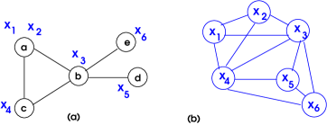
Figure 1: (Example 5) (a) Network polynomial optimization problem. (b) The intersection graph.

Example 6

Consider a knapsack problem $\min\{\,c^{T}x\ :\ a^{T}x\ \geq\ b,\ x\in\{0,1\}^{n}\,\}$. This is a NPO, using a star network on $n+1$ vertices, which has tree-width $1$. Yet, if $a_{j}\neq 0$ for all $j$, the intersection graph is a clique of size $n$. Note that we can restate $x\in\{0,1\}^{n}$ as $x_{j}(1-x_{j})=0,\,\forall j$.

In fact, even an AC-OPF instance, on a tree, can give rise to an intersection graph with high tree-width, because constraint (3e) or (3e) mirrors the intersection graph behavior in Example 6.

In the general case, in order to avoid the possible increase in tree-width going from the underlying graph to the intersection graph, we show that given a NPO problem on a graph of small tree-width, there is an equivalent NPO problem whose intersection graph also has small tree-width. As a result of this elaboration we obtain:

Theorem 7

Consider a network mixed-integer polynomial optimization problem over a graph $G$ of tree-width $\leq\omega$ and maximum-degree $D$, over $n$ variables, and where every polynomial $p_{u,v}$ has maximum degree $\leq\pi$. Suppose that the number of variables plus the number of constraints associated with any vertex of $G$ is at most $\Delta$. Given $0<\epsilon<1$, there is a linear programming formulation of size $O((D\pi/\epsilon)^{O(\Delta\omega)}\,n\,\log(\pi/\epsilon))$ that solves the problem within scaled tolerance $\epsilon$.

Here, “scaled tolerance” embodies the same notion of optimality and feasibility approximation as in Theorem 4. Later we will discuss why this approximation feature is needed. Further, we note that in the case of the AC-OPF problem we have $\Delta=5$ and $\pi=2$.

Corollary 8

There exist polynomial-time approximation schemes for the AC-OPF problem on graphs with bounded tree-width, and for the capacitated fixed-charge network flow problem on graphs with bounded tree-width.

Our third result is important toward the proof of Theorem 4 but is of independent interest. As we will see, the construction in Theorem 4 approximates a mixed-integer polynomially constrained problem with a polynomially constrained pure binary polynomially constrained problem. As a generalization, we study “general” binary problems, or GB for short, defined as follows.

• There are $n$ variables and $m$ constraints. For $1\leq i\leq m$, constraint $i$ is characterized by a subset $K[i]\subseteq\{1,\ldots,n\}$ and a set $S^{i}\subseteq\{0,1\}^{K[i]}$. Set $S^{i}$ is implicitly given by a membership oracle, that is to say a mechanism that upon input $y\in\{0,1\}^{K[i]}$, truthfully reports whether $y\in S^{i}$.

• The problem is to minimize a linear function $c^{T}x$, over $x\in\{0,1\}^{n}$, and subject to the constraint that for $1\leq i\leq m$ the sub-vector $x_{K[i]}$ is contained in $S^{i}$.

Any linear-objective, binary optimization problem whose constraints are explicitly stated can be recast in the form GB; e.g., each set $S^{i}$ could be described by a system of algebraic equations in the variables $x_{j}$ for $j\in K[i]$. GB problems are related to classical constraint satisfaction problems, however the terminology above will prove useful later. A proof of part (a) in the following result can be obtained using techniques in [39] (Section 8) although not explicitly stated there. We will outline this proof, which relies on the “cone of set-functions” approach of [42] and also present a new proof.

Theorem 9

Consider a GB problem whose intersection graph has tree-width $\leq\omega$.

• There is an exact linear programming formulation with $O(2^{\omega}n)$ variables and constraints, with $\{0,1,-1\}$-valued constraint coefficients.

• The formulation can be constructed by performing $2^{\omega}m$ oracle queries and with additional workload $O^{*}(\omega 2^{\omega}\sum_{t\in V(T)}|\left\{i\,:\,K[i]\subseteq Q_{t}\right\}|+\omega mn)=O^{*}(\omega 2^{\omega}mn+\omega^{2}2^{\omega}n)$, where the “*” notation indicates logarithmic factors in $m$ or $n$.

Note that the size of the formulation is independent of the number constraints in the given instance of GB. And even though we use the general setting of membership oracles, this theorem gives an exact reformulation, as opposed to Theorems 4 and 7, where an approximation is required unless P=NP. Theorem 9 has additional implications toward linear and polynomial binary optimization problems. We will examine these issues in Section 4. Regarding part (b) of the theorem, it can be shown that $2^{\omega}m$ is a lower bound on the number of oracle queries that any algorithm for solving GB must perform.

Theorem 9 describes an LP formulation for GB; the relevance of this focus was discussed above. Together with the reductions used to obtain Theorems 4 and 7 we obtain approximate LP formulations for polynomial (resp., network polynomial) mixed-integer problems. Of course, Theorem 9 also implies the existence of an algorithm for solving GB in time polynomial in $O(2^{\omega}(n+m))$. However one can also derive a direct algorithm of similar complexity using well-known, prior ideas on polynomial-time methods for combinatorial problems on graphs of bounded tree-width.

1.0.1 Prior work

There is a broad literature dating from the 1980s on polynomial-time algorithms for combinatorial problems on graphs with bounded tree-width. An early reference is [4]. Also see [2], [3], [18], [8], [14], [11] and from a very general perspective, [16]. These algorithms rely on “nonserial dynamic programming”, i.e., dynamic-programming on trees. See [1], [45], [9].

A parallel research stream concerns “constraint satisfaction problems”, or CSPs. Effectively, the feasibility version of problem GB is a CSP. One can also obtain an algorithm for problem GB, with similar complexity, and relying on similar dynamic programming ideas as the algorithms above, from the perspective of belief propagation on an appropriately defined graphical model. Another central technique is the tree-junction theorem of [40], which shows how a a set of marginal probability distributions on the edges of a hypertree can be extended to a joint distribution over the entire vertex set. Early references are [47], [23] and [22]. Also see [54], [19] (and references therein), and [55].

Turning to the integer programming context, [13] (also see the PhD thesis [57]) develop extended formulations for binary linear programs by considering the subset algebra of feasible solutions for individual constraints or small groups of constraints; this entails a refinement of the cone of set-functions approach of [42]. The method in [13] is similar to the one in this paper, in that here we rely on a similar algebra and on extended, or “lifted” reformulations for $0/1$ integer programs. The classical examples in this vein are the reformulation-linearization technique of [50], the cones of matrices method [42], the lift-and-project method of [6], and the moment relaxation methodology of [37]. See [38] for a unifying analysis; another comparison is provided in [5].

The work in [12] considers packing binary integer programs are considered, i.e. problems of the form

$$\max\{c^{T}x\,:\,Ax\leq b,\ x\in\{0,1\}^{n}\}$$ (6)

where $A\geq 0$ and integral and $b$ is integral. Given a valid inequality $\alpha x\geq\beta$, its associated graph is the subgraph of the intersection graph induced by $S=\{1\leq j\leq n:\,\alpha_{j}\neq 0\}$; i.e. it has vertex-set $S$ and there an edge $\{j,k\}\in S\times S$ whenever $a_{ij}\neq 0$ and $a_{ik}\neq 0$ for some row $i$.

In [12] it is shown that given and $\omega\geq 1$, the level-$\omega$ Sherali-Adams reformulation of (6) implies every valid inequality whose associated graph has tree-width $\leq\omega-1$. Further, if $A$ is $0/1$-valued, the same property holds when the associated graph has tree-width $\leq\omega$. As a corollary, given a graph $G$ with tree-width $\leq\omega$, the Sherali-Adams reformulation of the vertex packing linear program $\{x\in[0,1]^{V(G)}\,:\,x_{u}+x_{v}\leq 1\ \forall\,\{u,v\}\in E(G)\}$, which has $O(\omega n^{\omega+2})$ variables and constraints, is exact. As far as we know this is the first result linking tree-width and reformulations for integer programs. A different result which nevertheless appears related is obtained in [20].

In [54], binary polynomial optimization problems are considered, i.e problems as $\min\{\,c^{T}x\,:\,x\in\{0,1\}^{n},\ g_{i}(x)\geq 0,\ 1\leq i\leq M\}$ where each $g_{i}(x)$ is a polynomial. They show that if the tree-width of the intersection graph of the constraints is $\leq\omega$, then the level-$\omega$ Sherali-Adams or Lasserre reformulation of the problem is exact. Hence there is an LP formulation with $O(n^{\omega+2})$ variables and $O(n^{\omega+2}M)$ constraints.

A comprehensive survey of results on polynomial optimization and related topics is provided in [39]. Section 8 of [39] builds on the work in [38], which provides a common framework for the Sherali-Adams, Lovász-Schrijver and Lasserre reformulation operators. In addition to the aforementioned results related to problem GB (to which we will return later), [39] explicitly shows that the special case of the vertex-packing problem on a graph with $n$ vertices and tree-width $\leq\omega$ has a formulation of size $O(2^{\omega}n)$; this is stronger than the implication from [12] discussed above. Similarly, it is shown in [39] that the max-cut problem on a graph with $n$ vertices and tree-width $\leq\omega$ has a formulation of size $O(2^{\omega}n)$.

In the continuous variable polynomial optimization setting, [33], and [56] present methods for exploiting low tree-width of the intersection matrix e.g. to speed-up the sum-of-squares or moment relaxations of a problem. Also see [28] and Section 8 of [39]. [35] considers polynomial optimization problems as well. In abbreviated form, [35] shows that where $p$ is the tree-width of the intersection graph, there is a hierarchy of semidefinite relaxations where the $r^{th}$ relaxation ($r=1,2,\ldots...$) has $O(np^{2r})$ variables and $O(n+m)$ LMI constraints; further, as $r\rightarrow+\infty$ the value of the relaxation converges to the optimum. Also see [46] and [36].

Finally, there are a number of results on using lifted formulations for polynomial optimization problems, along the lines of the RLT methodology of [50]. See [52], [51] and references therein.

1.0.2 Organization of the paper

This paper is organized as follows. Mixed-integer polynomial optimization problems and a proof of Theorem 4 are covered in Section 2. Network mixed-integer polynomial optimization problems and Theorem 7 are addressed in Section 3. And finally, in Section 4, we will present a detailed analysis of the pure binary problems addressed by Theorem 9 and a proof of this result.

2 Mixed-integer polynomial optimization problems

In this section we consider mixed-integer polynomial optimization problems (PO) and prove a result (Theorem 15, below) that directly implies Theorem 4 given in the introduction. This proof will make use of the result in Theorem 9, to be proven in Section 4.

In what follows we will rely on a definition of tree-width which is equivalent to Definition 3. This definition makes use of the concept of tree-decomposition:

Definition 10

Let $G$ be an undirected graph. A tree-decomposition [48], [49] of $G$ is a pair $(T,Q)$ where $T$ is a tree and $Q=\{Q_{t}\,:\,t\in V(T)\}$ is a family of subsets of $V(G)$ such that

• For all $v\in V(G)$, the set $\{t\in V(T)\,:\,v\in Q_{t}\}$ forms a subtree $T_{v}$ of $T$, and

• For each $\{u,v\}\in E(G)$ there is a $t\in V(T)$ such that $\{u,v\}\subseteq Q_{t}$, i.e. $t\in T_{u}\cap T_{v}$.

The width of the decomposition is $\max\left\{|Q_{t}|\,:\,t\in V(T)\right\}\,-\,1$. The tree-width of $G$ is the minimum width of a tree-decomposition of $G$. See Example 11.

Example 11

(Tree-decomposition) Consider the intersection graph $G$ arising in Example 2. See Figure 2(a). A tree-decomposition with tree $T$ is shown in Figure 2(b)-(c).

Figure 2: A tree-decomposition. (a) Graph $G$. (b) Tree $T$. (c) Tree $T$ with subtrees $T_{v}$.

Since this definition relates a specific decomposition of the graph with its tree-width, many of the arguments we provide will rely on modifying or creating valid tree-decompositions that attain the desired widths.

We make some remarks pertaining to to the PO problem. Throughout we will use the definition of used in the introduction (formulation (2)). The $i^{th}$ constraint, for $1\leq i\leq m$, is given by $f_{i}(x)\geq 0$, where $f_{i}(x)$ is a has the form

$$f_{i}(x) = \sum_{\alpha\in I(i)}f_{i,\alpha}x^{\alpha}.$$ (7)

Here $I(i)\subseteq\{1,\ldots,n\}$ is a finite set, $f_{i,\alpha}$ is rational and $x^{\alpha}$ is a monomial in $x$:

$$x^{\alpha}\ =\ \prod_{j=1}^{n}x_{j}^{\alpha_{j}}.$$

Finally, for each $1\leq i\leq m$ we will denote as $\|f_{i}\|_{1}$ the 1-norm of the coefficients of polynomial $f_{i}(x)$, i.e

$$\|f_{i}\|_{1}=\sum_{\alpha\in I(i)}|f_{i,\alpha}|.$$

Any linear-objective mixed-integer polynomial optimization problem where the feasible region is compact can be reduced to the form (2) by appropriately translating and scaling variables.

Remark 12

A polynomial-optimization problem with nonlinear objective can trivially be made into the form (2), by (for example) using a new variable and two constraints to represent each monomial in the objective. Of course, such a modification may increase the tree-width of the intersection graph.

Now we precisely define what the intersection graph would be in this context.

Definition 13

Given an instance of problem PO, let its intersection graph $\Gamma$ be the undirected graph with $n$ vertices and where for $1\leq i\leq m$ the set

$$\{j\ :\ \alpha_{j}\neq 0,\ f_{i,\alpha}\neq 0,\ \alpha\in I(i)\}$$

induces a clique.

Definition 14

Consider an instance of problem PO.

• Given $\epsilon>0$, we say a vector $x\in\{0,1\}^{p}\times[0,1]^{n-p}$ is scaled-${\epsilon}$ feasible if

  $$f_{i}(x) \geq -\epsilon\|f_{i}\|_{1},\quad 1\leq i\leq m.$$ (8)

• We set ${\pi\doteq\max_{1\leq i\leq m}\max_{\alpha\in I(i)}\sum_{j=p+1}^{n}\alpha_{j}}$.

We will prove the following result:

Theorem 15

Given an instance of PO, let $\omega$ be the width of a tree-decomposition of the intersection graph. For every $0<\epsilon<1$ there is a linear program

$$LP\,:\,\min\{\hat{c}^{T}y\,:\,\hat{A}y\geq\hat{b}\}$$

with the following properties:

• The number of variables and constraints is $O\left((2\pi/\epsilon)^{\omega+1}n\log(\pi/\epsilon)\right)$, and all coefficients are of polynomial size.

• Given any feasible solution $x$ to PO, there is a feasible solution $y$ to LP with

  $$\hat{c}^{T}y\leq c^{T}x+\epsilon\|c\|_{1}.$$

• Given an optimal solution $y^{*}$ to LP, we can construct $x^{*}\in\{0,1\}^{p}\times[0,1]^{n-p}$ such that:

  1. $$x^{*} \epsilon$$ is scaled- feasible for PO, and

  2. $$c^{T}x^{*}\ =\ c^{T}y^{*}.$$

Remark 16

Assume PO is feasible. Then (b) shows LP is feasible and furthermore by (c) solving LP yields a near-feasible solution for PO which may be superoptimal, but is not highly suboptimal. Condition (a) states that the formulation $LP$ is of pseudo-polynomial size.

To prove Theorem 15 we will rely on a technique used in [26]; also see [10] and [21], [29] and citations therein. Suppose that $0\leq r\leq 1$. Then we can approximate $r$ as a sum of inverse powers of $2$. Let $0<\gamma<1$ and

$$L\ =\ L(\gamma)\ \doteq\ \lceil\log_{2}\gamma^{-1}\rceil.$$

Then there exist $0/1$-values $z_{h}$, $1\leq h\leq L$, with

$$\sum_{h=1}^{L}2^{-h}z_{h}\ \leq\quad r\quad\leq\ \sum_{h=1}^{L}2^{-h}z_{h}\,+\,2^{-L}\ \leq\sum_{h=1}^{L}2^{-h}z_{h}\,+\,\gamma\,\leq\,1.$$ (9)

Next we approximate problem PO with a problem of type GB. For each $1\leq i\leq m$ and $\alpha\in I(i)$ we write

$$Z(i,\alpha)=\{j\ :\alpha_{j}\neq 0,\ 1\leq j\leq p\}.$$

In other words, set $Z(i,\alpha)$ is the set given by the indices of the binary variables for PO that appear explicitly in monomial $x^{\alpha}$; thus for $j\in Z(i,\alpha)$ we have $x_{j}^{\alpha_{j}}=x_{j}$. Let

$$\mbox{ {\boldmath${\delta\ =\ \delta(\gamma,\pi)\ \doteq\ 1-(1-\gamma)^{\pi}}$}}.$$ (10)

The theorem will be obtained by using the following formulation, for appropriate $\gamma=\gamma(\epsilon):$

$$\mbox{(GB$(\gamma)$)}: \min~{}\sum_{j=1}^{p}c_{j}x_{j}\ +\ \sum_{j=p+1}^{n}c_{j}\left(\sum_{h=1}^{L}2^{-h}z_{j,h}\right)$$

s.t. $$\sum_{\alpha\in I(i)}f_{i,\alpha}\left[\,\prod_{j\in Z(i,\alpha)}x_{j}\,\prod_{j=p+1}^{n}\left(\sum_{h=1}^{L}2^{-h}z_{j,h}\right)^{\alpha_{j}}\,\right]\ \geq\ -\delta\,\|f_{i}\|_{1},\quad 1\leq i\leq m$$

$$x_{j}\,\in\,\{0,1\},\ 1\leq j\leq p,\quad z_{j,h}\,\in\,\{0,1\},\ \forall j\in\{p+1,\ldots,n\},\ 1\leq h\leq L.$$

Remark. This formulation replaces, in PO, each continuous variable $x_{j}$ with a sum of powers of $1/2$, using the binary variables $z_{j,h}$ in order to effect the approximation (9).

To prove the desired result we first need a technical property.

Lemma 17

Suppose that for $1\leq k\leq r$ we have values $u_{k}\geq 0,\ v_{k}\geq 0,\ q_{k}\in\mathbb{Z}_{+}$ with $u_{k}+v_{k}\leq 1$. Then

$$\prod_{k=1}^{r}(u_{k}+v_{k})^{q_{k}}\,-\,\prod_{k=1}^{r}u_{k}^{q_{k}}\ \leq\ 1\,-\,\prod_{k=1}^{r}(1-v_{k})^{q_{k}}.$$

Proof. Take any fixed index $1\leq i\leq r$. The expression

$$\prod_{k=1}^{r}(u_{k}+v_{k})^{q_{k}}-\prod_{k=1}^{r}(u_{k})^{q_{k}}$$

is a nondecreasing function of $u_{i}$ when all $u_{k}$ and $v_{k}$ are nonnegative, and so in the range $0\leq u_{i}\leq 1-v_{i}$ it is maximized when $u_{i}=1-v_{i}$.   

Using this fact, we can now show:

Lemma 18

• Suppose $\tilde{x}$ is a feasible for PO. Then there is feasible solution for GB$(\gamma)$ with objective value at most $c^{T}\tilde{x}\ +\ \ \delta\|c\|_{1}$.

• Conversely, suppose $(\hat{x},\hat{z})$ is feasible for GB$(\gamma)$. Writing, for each $p+1\leq j\leq n$, $\hat{x}_{j}=\sum_{h=1}^{L}2^{-h}\hat{z}_{j,h}$, we have that $\hat{x}$ is scaled-$\delta$-feasible for PO and $c^{T}\hat{x}\,=\,\sum_{j=1}^{n}c_{j}\left(\sum_{h=1}^{L}2^{-h}\hat{z}_{j,h}\right)$.

Proof. (a) For each $j$ choose binary values $\tilde{z}_{j,h}$ so as to attain the approximation in (9). Then for each $1\leq i\leq m$ and $\alpha\in I(i)$ we have

$$\prod_{j=p+1}^{n}\left(\sum_{h=1}^{L}2^{-h}\tilde{z}_{j,h}\right)^{\alpha_{j}}\ \leq\ \prod_{j=p+1}^{n}\tilde{x}_{j}^{\alpha_{j}}\ \leq\ \prod_{j=p+1}^{n}\left(\sum_{h=1}^{L}2^{-h}\tilde{z}_{j,h}\right)^{\alpha_{j}}\ +\ \delta.$$

Here the left-hand inequality is clear, and the right-hand inequality follows from Lemma 17 and the definition (10) of $\delta$. Thus $\tilde{z}$ is feasible for $GB(\gamma)$ and the second assertion is similarly proved.
(b) Follows by construction.   

We can now complete the proof of Theorem 15. Given an instance of problem PO together with a tree-decomposition of its intersection graph, of width $\omega$, we consider formulation GB$(\gamma)$ for $\gamma=\epsilon\pi^{-1}$. As an instance of GB, the formulation has at most $nL(\gamma)$ variables and its intersection graph has width at most $(\omega+1)L(\gamma)-1$. To see this point, consider a tree-decomposition $(T,Q)$ of the intersection graph for PO. Then we obtain a tree-decomposition $(T,\breve{Q})$ for GB$(\gamma)$ by setting, for each $t\in V(T)$,

$$\breve{Q}_{t}\ =\ \{z_{j,h}\,:\,1\leq h\leq L(\gamma),\,j\in Q_{t}\}.$$

We then apply, to this instance of GB, Theorem 9. We obtain an exact, continuous linear programming reformulation for GB($\gamma$) with

$$O(\,2^{(\omega+1)L(\gamma)}\,n\,L(\gamma)\,)\ =\ O((2\pi/\epsilon)^{\omega+1}n\log(\pi/\epsilon)\,)$$

variables and constraints. In view of Lemma 18, and the fact that $\delta=1-(1-\gamma)^{\pi}\leq\pi\gamma=\epsilon$, the proof of Theorem 15 is complete.

2.0.1 Can the dependence on $\epsilon$ be improved upon?

A reader may wonder why or if “exact” feasibility (or optimality) for PO cannot be guaranteed. From a trivial perspective, we point out that there exist simple instances of PO (in fact convex, quadratically constrained problems) where all feasible solutions have irrational coordinates. Should that be the case, if any algorithm outputs an explicit numerical solution in finite time, such a solution will be infeasible. A different perspective is that discussed in Example 6. As shown there we cannot expect to obtain an exact optimal solution in polynomial time, even in the bounded tree-width case, and even if there is a rational optimal solution, unless P = NP.

To address either issue one can, instead, attempt to output solutions that are approximately feasible. The approximation scheme given by Theorem 15 has two characteristics: first, it allows a violation of each constraint by $\epsilon$ times the 1-norm of the constraint, and second, the running time is pseudopolynomial in $\epsilon^{-1}$. One may wonder if either characteristic can be improved. For example, one might ask for constraint violations that are at most $\epsilon$, independent of the 1-norm of the constraints. However this is not possible even for a fixed value of $\epsilon$, unless P=NP. For completeness, we include a detailed analysis of this fact in Section A of the Appendix. Intuitively, if we were allowed to approximately satisfy every constraint with an error that does not depend on the data, we could appropriately scale constraint coefficients so as to obtain exact solutions to NP-hard problems.

Similarly, it is not possible to reduce the pseudopolynomial dependency on $\epsilon^{-1}$ in general. The precise statement is given in Section A of the Appendix as well, and the intuitive reasoning is similar: if there was a formulation of size polynomially dependent on $\log(\epsilon^{-1})$ (and not on $\epsilon^{-1}$) we could again solve NP-hard problems in polynomial time.

3 Network mixed-integer polynomial optimization problems

Here we return to the network polynomial optimization problems presented in the introduction, and provide a proof of Theorem 7. We will first motivate the technical approach to be used in this proof. Consider an NPO instance with graph $G$. For each $u\in V(G)$, $X_{u}$ denotes the set of variables associated with $u$ and $\deg_{G}(u)$ is the degree of $u$. At each $u\in V(G)$ we have a set of polynomial constraints of the general form

$$\sum_{\{u,v\}\in\delta(u)}p^{k}_{u,v}(X_{u}\cup X_{v})\ \geq\ 0,\quad\quad k=1,\ldots,K_{u}$$ (12)

associated with $u$, where each $p^{k}_{u,v}$ is a polynomial (possibly $K_{u}=0$). Without loss of generality we assume that, for every $u$ and $k=1,\ldots,K_{u}$ no two polynomials $p^{k}_{u,v}$ $\{u,v\}\in\delta(u)$ in (12) have a common monomial. If that were not the case, we could always combine the common monomials and assign them to a single $p^{k}_{u,v}$. This allows us to have

$$\left\|\sum_{\{u,v\}\in\delta(u)}p^{k}_{u,v}\right\|_{1}=\sum_{\{u,v\}\in\delta(u)}\left\|p^{k}_{u,v}\right\|_{1},\quad k=1,\ldots,K_{u}.$$ (13)

Now define

$$\Delta \doteq \max_{v\in V(G)}\{\,|X_{v}|+K_{v}\,\},\mbox{ and}$$ (14a)

$$D \doteq \max_{v\in V(G)}\{\deg_{G}(v)\}.$$ (14b)

As discussed above, we cannot reduce Theorem 7 to Theorem 4 because even if the graph $G$ underlying the NPO problem has small tree-width, the same may not be the case for the intersection graph of the constraints: a constraint (12) can yield a clique of size $|\delta(u)|$ in the intersection graph (or larger, if e.g. some $|X_{v}|>1$). In other words, high degree vertices in $G$ result in large tree-width of the intersection graph.

Figure 3: Vertex splitting.

One immediate idea is to employ the technique of vertex splitting. Suppose $u\in V(G)$ has degree larger than three and consider a partition of $\delta(u)$ into two sets $A_{1}$, $A_{2}$. We obtain a new graph $G^{\prime}$ from $G$ by replacing $u$ with two new vertices, $u_{1}$ and $u_{2}$, introducing the edge $\{u_{1},u_{2}\}$ and replacing each edge $\{u,v\}\in A_{S}$ (for $S=1,2$) with $\{u_{S},v\}$. See Figure 3.

Repeating this procedure, given $u\in V(G)$ with $\deg_{G}(u)>3$ we can replace $u$ and the set of edges $\delta(u)$ with a tree, where each internal vertex will have degree equal to three. To illustrate this construction, consider the example on Figure 4.

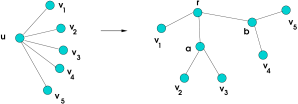
Figure 4: Example of complete vertex splitting.

In this figure, a degree-5 node $u$ and the set of edges $\{(u,v_{i})\,:\,1\leq i\leq 5\}$ is converted into a tree with three internal vertices ($r,a$ and $b$) and with each edge $(u,v_{i})$ having a corresponding edge in the tree. To keep the illustration simple, suppose there is a unique constraint of the form

$$\sum_{i=1}^{5}p_{u,v_{i}}(X_{u}\cup X_{v_{i}})\ \geq\ 0.$$ (15)

associated with $u$ in the given NPO. This constraint can be transformed into the following system of constraints:

$$p_{u,v_{2}}(X_{u}\cup X_{v_{2}}) = \|p_{u,v_{2}}\|_{1}\,(y^{+}_{v_{2}}\,-\,y^{-}_{v_{2}})$$ (16a)

$$p_{u,v_{3}}(X_{u}\cup X_{v_{3}}) = \|p_{u,v_{3}}\|_{1}\,(y^{+}_{v_{3}}\,-\,y^{-}_{v_{3}})$$ (16b)

$$(\|p_{u,v_{2}}\|_{1}+\|p_{u,v_{3}}\|_{1})(y^{+}_{a}-y^{-}_{a}) = \|p_{u,v_{2}}\|_{1}\,(y^{+}_{v_{2}}\,-\,y^{-}_{v_{2}})\ +\ \|p_{u,v_{3}}\|_{1}(y^{+}_{v_{3}}\,-\,y^{-}_{v_{3}})$$ (16c)

$$p_{u,v_{4}}(X_{u}\cup X_{v_{4}}) = \|p_{u,v_{4}}\|_{1}\,(y^{+}_{v_{4}}\,-\,y^{-}_{v_{4}})$$ (16d)

$$p_{u,v_{5}}(X_{u}\cup X_{v_{5}}) = \|p_{u,v_{5}}\|_{1}\,(y^{+}_{v_{5}}\,-\,y^{-}_{v_{5}})$$ (16e)

$$(\|p_{u,v_{4}}\|_{1}+\|p_{u,v_{5}}\|_{1})(y^{+}_{b}-y^{-}_{b}) = \|p_{u,v_{4}}\|_{1}\,(y^{+}_{v_{4}}\,-\,y^{-}_{v_{4}})\ +\ \|p_{u,v_{5}}\|_{1}(y^{+}_{v_{5}}\,-\,y^{-}_{v_{5}})$$ (16f)

$$p_{u,v_{1}}(X_{u}\cup X_{v_{1}}) = \|p_{u,v_{1}}\|_{1}\,(y^{+}_{v_{1}}\,-\,y^{-}_{v_{1}})$$ (16g)

$$\left(\sum_{j=1}^{5}\|p_{u,v_{j}}\|_{1}\right)y^{+}_{r} = \|p_{u,v_{1}}\|_{1}\,(y^{+}_{v_{1}}\,-\,y^{-}_{v_{1}})+(\|p_{u,v_{2}}\|_{1}+\|p_{u,v_{3}}\|_{1})(y^{+}_{a}-y^{-}_{a})$$

$$\hskip 14.45377pt+(\|p_{u,v_{4}}\|_{1}+\|p_{u,v_{5}}\|_{1})(y^{+}_{b}-y^{-}_{b})$$

$$0\leq y^{+},y^{-}\leq 1.$$

Clearly, substituting (15) associated with $u$ with the equivalent system (16) yields an equivalent NPO where

$$X_{a} = X_{u}\cup\{y^{+}_{a},y^{-}_{a},y^{+}_{v_{2}},y^{-}_{v_{2}},y^{+}_{v_{3}},y^{-}_{v_{3}}\}$$

$$X_{b} = X_{u}\cup\{y^{+}_{b},y^{-}_{b},y^{+}_{v_{4}},y^{-}_{v_{4}},y^{+}_{v_{4}},y^{-}_{v_{4}}\}$$

$$X_{r} = X_{u}\cup\{y^{+}_{r},y^{+}_{v_{1}},y^{-}_{v_{1}}\}$$

and constraints (16a), (16b) and (16c) are associated with vertex $a$, constraints (16d), (16e) and (16f) are associated with vertex $b$, and constraints (16g) and (16) are associated to vertex $r$. It is important to notice that we do not associate variables $y^{+}_{v_{i}}$ and $y^{-}_{v_{i}}$ with nodes $v_{i}$, but rather with internal vertices of the tree. The motivation for this detail is that vertices $v_{i}$ may have degree greater than three, and would (later) be split as well. Thus, adding new variables to $X_{v_{i}}$ might create difficulties when defining the general procedure. This is avoided by keeping the same sets $X_{v_{i}}$ associated with $v_{i}$ after a neighbor of $v_{i}$ is split, as in the previous example.

We indicate the general formal procedure next; however we warn the reader in advance that this strategy may not directly deliver Theorem 7 because the splitting process may (if not chosen with care) produce a graph with much higher tree-width than $G$. This is a technical point that we will address later (Section 3.0.1).

To describe the general procedure we use the following notation: given a tree $T$, an edge of $T$ is called pendant if it is incident with a leaf, and non-leaf vertex is called internal; the set of internal vertices is denoted by $int(T)$. Now fix a vertex $u$ of $G$ such that $\deg_{G}(u)>3$. Let $\hat{T}_{u}$ be an arbitrary tree where

• $int(\hat{T}_{u})\cap V(G)=\emptyset$, $\hat{T}_{u}$ has $\deg_{G}(u)$ leaves, and for each edge $\{u,v\}\in E(G)$ there is one pendant edge $\{i,v\}$ of $\hat{T}_{u}$, and

• each internal vertex of $\hat{T}_{u}$ has degree equal to three,

Then completely splitting $u$ using $\hat{T}_{u}$ yields a new graph, $\breve{G}$ where $V(\breve{G})\ =\ (V(G)-u)\cup int(\hat{T}_{u})$, and $E(\breve{G})\ =\ (E(G)-\delta_{G}(u))\cup E(\hat{T}_{u})$.

To obtain an NPO system in $\breve{G}$ equivalent to the original system, we replace each constraint (12) that is associated with $u$ with a family of constraints associated with the internal vertices of $\hat{T}_{u}$. To do so, pick an arbitrary non-leaf vertex $r$ of $\hat{T}_{u}$ and view $\hat{T}_{u}$ as rooted at $r$ (i.e., oriented away from $r$), and define, for each internal vertex $i$ of $\hat{T}_{u}$ and $k=1,\ldots,K_{u}$,

$$\nu_{i}^{k} = \sum\left\{\|p^{k}_{u,v}\|_{1}\,:\,(u,v)\in\delta(u),\,\mbox{$v$ a descendant of $i$ in $\hat{T}_{u}$}\right\}$$

Then, for each internal vertex $i$ of $\hat{T}_{u}$ we have

• All variables in $X_{u}$ are associated with $i$.

• For each $k=1,\ldots,K_{u}$, if $i\neq r$ we additionally associate two variables, $y^{+}_{i,k},~{}y^{-}_{i,k}\in[0,1]$, and if $i=r$ we only add $y^{+}_{r,k}\in[0,1]$ with $i$. If $i$ has a child $v$ that is a leaf, and hence $\{u,v\}\in\delta(u)$, then we associate two additional variables $y^{+}_{v,k},~{}y^{-}_{v,k}\in[0,1]$ with $i$.

• If $i\neq r$, then letting $j,l$ be its children we write the following constraints associated with $i$:

  $$\nu^{k}_{j}(y^{+}_{j,k}-y^{-}_{j,k})+\nu^{k}_{l}(y^{+}_{l,k}-y^{-}_{l,k})\,=\,\nu^{k}_{i}(y^{+}_{i,k}-y^{-}_{i,k})\quad\quad 1\leq k\leq K_{u}.$$ (17)

  If on the other hand $i=r$, let $j,l,h$ be its children. Then we write

  $$\nu^{k}_{r}y^{+}_{r,k}-\sum_{s=j,l,h}\nu^{k}_{s}(y^{+}_{s,k}-y^{-}_{s,k})\ =\ 0\quad\quad 1\leq k\leq K_{u}.$$ (18)

Finally, given a leaf $v$ of $\hat{T}_{u}$ with parent $i$, then by construction $\{u,v\}\in\delta(u)$. Then we add the following constraints, associated with $i$ (not $v$),

$$\|p^{k}_{u,v}\|_{1}(y^{+}_{v,k}-y^{-}_{v,k})\ -\ p^{k}_{u,v}(X_{u}\cup X_{v})\ =\ 0\quad\quad 1\leq k\leq K_{u}.$$ (19)

Let us denote the initial NPO by $P$. Since the sum of constraints (17), (18) and (19) is (12) we have obtained an NPO equivalent to $P$. Note that for any $v\in V(G)-u$ the degree of $v$ is unchanged, as is the set $X_{v}$ and the set of constraints associated with $v$. Thus, proceeding in the above manner with every vertex $u\in V(G)$ with $\deg_{G}(u)>3$ we will obtain the final graph (which we denote by $G^{\prime}$) of maximum degree $\leq 3$ and an NPO, denoted by $P^{\prime}$ which is equivalent to $P$.

The following lemmas lay out the strategy that we will follow to prove Theorem 7. To prepare for these, we need a technical remark, which follows from the definition of tree-decomposition.

Remark 19

Suppose that $(T,Q)$ is a tree-decomposition of a graph $H$. Suppose a subset of vertices $S$ induces a connected subgraph of $H$. Then

$$\{t\in V(T)\,:\,Q_{t}\cap S\neq\emptyset\}$$

induces a subtree of $T$.

Returning to our construction, we assume that we have a tree decomposition $(T^{\prime},Q^{\prime})$ of $G^{\prime}$. Note that each vertex $v$ of $G^{\prime}$ is derived from some vertex, say $u(v)\in V(G)$ and the set of variables associated with $v$ under $P^{\prime}$ is a copy of $X_{u(v)}$, together with the $y^{+}$ and $y^{-}$ variables introduced above. We have one pair of such variables per each constraint (12) associated with $u(v)$ and an extra pair when $v$ is the parent of a leaf in $\hat{T}_{u(v)}$.

We consider now the following pair: $(T^{\prime},\tilde{Q}^{\prime})$, with each $\tilde{Q}^{\prime}_{t}$ $t\in T^{\prime}$ defined as follows. For each $v\in Q^{\prime}_{t}$, the set $\tilde{Q}^{\prime}_{t}$ will include (1) $X_{u(v)}$ together with the $y^{+}$ and $y^{-}$ variables associated with $v$ or its children in $\hat{T}_{u(v)}$. This can include up to $|X_{v}|+7K_{v}$ variables for each $v$ (the bound is tight at the root $r$ which is the only internal vertex with three children; further we are counting $y^{+}_{r}$). (2) If $v$ is the parent of leaf in $\hat{T}_{u(v)}$, say $w$, then we also add to $\tilde{Q}^{\prime}_{t}$ the set $X_{u(w)}$. Further, the number of constraints associated with internal vertices is clearly $\leq 3K_{v}$.

Lemma 20

The pair $(T^{\prime},\tilde{Q}^{\prime})$ is a tree-decomposition of the intersection graph of $P^{\prime}$.

Proof. We need to show that (a) for any variable $x_{j}$ of $P^{\prime}$. the set of vertices $t$ of $T^{\prime}$ such that $\tilde{Q}^{\prime}_{t}$ contains $x_{j}$ forms a subtree of $T^{\prime}$, and (b) that for any edge $\{x_{k},x_{j}\}$ of the intersection graph of $P^{\prime}$ the pair $x_{k},x_{j}$ are found in a common set $\tilde{Q}^{\prime}_{t}$.

Part (b) follows directly from the construction of the sets $\tilde{Q}^{\prime}_{t}$, as each of the constraints (17), (18) and (19) involve only one internal node and its children, including the case when some children are leaves, which is accounted for in (2).

As for part (a), the statement is clear if $x_{j}$ is one of the $y^{+},y^{-}$ variables. If, instead, $x_{j}$ is contained in some set $X_{u(v)}$ then $x_{j}$ is associated with every vertex in $\hat{T}_{u(v)}$. By definition of NPOs, the set of $w$ vertices of $G$ such that $x_{j}\in X_{w}$ forms a connected subgraph of $G$. It follows that the set of vertices $v$ of $G^{\prime}$ such that $x_{j}$ is associated with $v$ in $P^{\prime}$ forms a connected subgraph of $G^{\prime}$. Part (a) now follows from Remark 19.   

Lemma 21

Suppose that $G^{\prime}$ has tree-width $\leq W$. Then the intersection graph of $P^{\prime}$ has tree-width $\leq 7\Delta(W+1)-1$.

Proof. Consider a tree-decomposition $(T^{\prime},Q^{\prime})$ of $G^{\prime}$ of width $\leq W$ and construct $\tilde{Q}^{\prime}$ as before. We claim that the width of $(T^{\prime},\tilde{Q}^{\prime})$ is at most $7\Delta(W+1)-1$. But this is clear since $|Q^{\prime}_{t}|\leq W+1$, and each $v\in Q^{\prime}_{t}$ will contribute at most three extra sets of the type $X_{w}$ for some $w$, along with the $|X_{v}|+7K_{v}$ quantities stated before. Hence,

$$|\tilde{Q}^{\prime}_{t}|\leq 7\Delta(W+1)$$

as desired.   

Lemma 22

Given $0<\epsilon<1$, there is a linear programming formulation LP for the NPO problem on $G$, of size $O((D\pi/\epsilon)^{O(\Delta W)}\,n\,\log\epsilon^{-1})$, that solves the problem within scaled tolerance $\epsilon$.

Proof. Suppose we apply Theorem 15 to problem $P^{\prime}$, for a given tolerance $0<\theta<1$. Note that, in order to do so rigorously, equations (17) and (19) must be first transformed to 2 inequality constraints each.

The resulting linear programming formulation, LP, will have size $O((2\pi/\theta)^{O(\Delta W)}\,n\,\log\theta^{-1})$ and will yield $\theta$-approximate solutions to $P^{\prime}$. In particular, these solutions may violate a constraint of $P^{\prime}$ by an amount proportional to the $1$-norm of the constraint, times $\theta$, as guaranteed by Theorem 15.

Consider a constraint (12) of problem $P$, associated with a vertex $u$ of $G$, with 1-norm denoted by $\|p_{u}^{k}\|_{1}$. In $P^{\prime}$ this constraint has been replaced by a family $\mathcal{F}$ of constraints, one per each vertex of $\hat{T}_{u}$ whose sum yields (12). Simple algebra shows that the solution to LP may violate (12) by an amount equal to the sum of violations of the constraints in $\mathcal{F}$. The $1$-norm of each such constraint is at most $4\|p_{u}^{k}\|_{1}$, since if $i$ is an internal node of some tree $\hat{T}_{u}$ with children $j,l$ then

$$\nu_{i}^{k}=\nu_{j}^{k}+\nu_{l}^{k}$$

and for a root node $r$ with children $j,h,l$

$$\|p_{u}^{k}\|_{1}=\nu_{r}^{k}=\nu_{j}^{k}+\nu_{h}^{k}+\nu_{l}^{k}$$

by (13). Since $\hat{T}_{u}$ has $\deg_{G}(u)$ leaves and all internal vertices have degree 3, it can be easily shown that it must have less than $2\deg_{G}(u)$ vertices in total. From this it follows that the LP solution violates (12) by at most $8\|p_{u}^{k}\|_{1}\deg_{G}(u)\theta$. Choosing $\theta=(8D)^{-1}\epsilon$, and noting that for a constant $c$

$$(cD\pi/\epsilon)^{O(\Delta E)}\in O(D\pi/\epsilon)^{O(\Delta E)})$$

yields the desired result.   

As per Lemma 22, these constructions obtain Theorem 7 provided that we find a vertex splitting with $W=O(\omega)$. As discussed in the next section, this condition may fail to hold under an arbitrary vertex splitting, and some care is needed.

3.0.1 Finding good vertex splittings

Consider the example given in Figure 5.

Figure 5: Incorrect vertex splitting.

Here the vertices of the graph shown in (a) are arranged into $k>1$ columns. The odd-numbered columns have $k$ vertices each, which induce a path, while the even-numbered columns have a single vertex which is adjacent to all vertices in the preceding and following columns. It can be shown that this graph has tree-width $3$. In (b) we show the outcome after splitting vertices so that the maximum degree is four. This second graph has tree-width $k$, and further splitting the degree-four vertices will not change this fact.

Figure 6: Correct vertex splitting of graph in Figure 5(a).

In contrast to this situation, suppose that we split the graph in Figure 5(a) in two steps as shown in Figure 6. The tree-width of the final graph is also 3. The difference between Figures 5 and 6 is explained by the fact that the splitting initiated by the “first step” in Figure 6 exploits the tree-decomposition of width $3$ of the graph Figure 5(a).

Next we turn to a formal approach that produces the desired outcome in the general setting. Given a graph $G$, a simplification of $G$ will be graph $\bar{G}$ obtained by a sequence of complete vertex splittings, such that the maximum degree of a vertex in $\bar{G}$ is $\leq 3$. The following Lemma will show how to obtain a simplification of a graph via a vertex splitting that maintains tree-width up to a constant factor. In the proof, the trees $\hat{T}_{u}$ that yield the general splitting procedure stated above, will be explicitly defined.

Lemma 23

Let $G$ be an undirected graph and $(T,Q)$ a tree-decomposition of $G$ of width $Z$. Then there is a simplification $\bar{G}$ of $G$ and a tree-decomposition $(\bar{T},\bar{Q})$ of $\bar{G}$ of width at most $2Z+1$.

Proof. We first modify $(T,Q)$ in a sequence of steps.

Step 1. For any edge $e=\{u,v\}\in E(G)$, choose an arbitrary $t\in V(T)$ with $e\subseteq Q_{t}$. Then we modify $T$ by adding to $T$ a new vertex, $t^{e}$ and the edge $\{t^{e},t\}$. Further, we set $Q_{t^{e}}=\{u,v\}$.

Step 2. Without loss of generality, every vertex of $T$ has degree at most $3$. To attain this condition, consider any $t\in V(T)$ with $\delta_{T}(t)=\{s_{1},\ldots,s_{d}\}$ (say) where $d>3$. Then we alter $T$ by replacing $t$ with two vertices adjacent vertices $t^{1}$ and $t^{2}$, such that $t^{1}$ is also adjacent to $s_{1}$ and $s_{2}$ and $t^{2}$ is adjacent to $s_{3},\ldots,s_{d}$. Finally, we set $Q_{t^{1}}=Q_{t^{2}}=Q_{t}$. Continuing inductively we will attain the desired condition.

Step 3. For any vertex $u\in V(G)$ let $T_{u}$ be the subtree of $T$ consisting of vertices $t$ with $u\in Q_{t}$, and $\breve{T}_{u}$ be the subtree of $T_{u}$ that spans $\{t^{e}\,:\,e\in\delta_{G}(u)\}$ (which is a subset of the leaves of $T_{u}$). Then we modify $(T,Q)$ by replacing $T_{u}$ with $\breve{T}_{u}$, yielding a new tree-decomposition of same or smaller width. In other words, without loss of generality every leaf of $T_{u}$ is of the form $t^{e}$ for some $e\in\delta_{G}(u)$.

We can now describe our vertex splitting scheme. Consider $u\in V(G)$ with $\deg_{G}(u)>3$. We say that a vertex of $T_{u}$ is blue if it is either a leaf or of degree three in $T_{u}$. Now we form the tree $\hat{T}_{u}$ whose vertex-set is the set of blue vertices of $T_{u}$, and whose edge-set is obtained as follows. By construction, $E(T_{u})$ can be partitioned into a set of paths whose endpoints are blue and which contain no other blue vertices. For each such path, with endpoints $a$ and $b$ (say), the tree $\hat{T}_{u}$ will contain the edge $\{a,b\}$ (in other words, $T_{u}$ can be obtained from $\hat{T}_{u}$ by subdividing some edges and so $T_{u}$ and $\hat{T}_{u}$ are topologically equivalent). Note that $\hat{T}_{u}$ has $\deg_{G}(u)$ leaves, each internal vertex with degree 3, and for each edge $\{u,v\}\in E(G)$ there is one pendant edge, as needed.

Let $\breve{G}$ be the graph obtained by the complete splitting of $u$ using $\hat{T}_{u}$. For each internal vertex $t\in V(\hat{T}_{u})$ we name $u^{t}$ the corresponding new vertex in $\breve{G}$, to emphasize that each non-leaf vertex in $\hat{T}_{u}$ will create a copy of $u$ (recall that the leaves in $\hat{T}_{u}$ will correspond to the neighbors of $u$). This operation does not change the degree of any vertex $v\in V(G)$ with $v\neq u$. The eventual graph $\bar{G}$ in the proof will be obtained by applying complete splittings at every vertex of degree $>3$ in $G$.

Returning to $\breve{G}$ we construct a tree decomposition $(T,\breve{Q})$ as follows. First, let us regard the tree $T_{u}$ as rooted at some internal blue vertex $r(u)$. For a vertex $t\in V(T_{u})$ let $R_{u}(t)$ be the closest blue ancestor of $t$ in $T_{u}$; we write $R_{u}(r(u))=r(u)$. Then, for $t\in V(T)$, we set

$$\breve{Q}_{t}\ =\ \left\{\begin{array}[]{ll}(Q_{t}-u)\cup\{u^{R_{u}(t)}\},&\mbox{if $t\in V(T_{u})$ and $\deg_{T_{u}}(t)=2$ },\\ (Q_{t}-u)\cup\{u^{t},u^{R_{u}(t)}\},&\mbox{if $t\in V(T_{u})$ and $\deg_{T_{u}}(t)\neq 2$},\\ Q_{t},&\mbox{if $t\notin V(T_{u})$.}\end{array}\right.$$ (23)

Now we argue that $(T,\breve{Q})$ is a tree-decomposition of $\breve{G}$. To see this, note that if $t\in V(\hat{T}_{u})$ then $u^{t}\in\breve{Q}_{s}$ iff $s=t$ or $s$ is a child of $t$ in $\hat{T}_{u}$, thus the endpoints of any edge $\{u^{t},u^{s}\}$, where $t$ is the parent of $s$, will be contained in $\breve{Q}_{s}$. Further, for any edge of $e=\{u,v\}$ of $G$, by Step 3 above there will be a leaf $t^{e}$ of $T_{u}$ such that the edge $\{t^{e},R_{u}(t^{e})\}\in E(\hat{T}_{u})$. This corresponds to a pendant edge $\{u^{R(t^{e})},v\}\in E(\breve{G})$ and by construction both $v\in\breve{Q}_{t^{e}}$ and $u^{R(t^{e})}\in\breve{Q}_{t^{e}}$. The fact that every vertex in $\breve{G}$ induces a connected subgraph in $T$ can be easily verified. This completes the argument $(T,\breve{Q})$ is a tree-decomposition of $\breve{G}$.

Notice that for $v\in V(G)$ with $v\neq u$, the subtree $T_{v}$ is the same in $(T,Q)$ and $(T,\breve{Q})$. Thus, applying the complete splitting of every vertex of $G$ of degree greater than three, and modifying the tree-decompostion as in (23) will produce a tree-decomposition $(T,\bar{Q})$ of the final graph $\bar{G}$.

By construction, for each $t\in V(T)$ we obtain $\bar{Q}_{t}$ from $Q_{t}$ by replacing each element with (at most) two new elements. Thus, since $|Q_{t}|\leq Z+1$, the width of $(T,\breve{Q})$ is at most $2(Z+1)-1$.   

4 Pure binary problems

In this section we will consider Theorem 9 of the Introduction. As we mentioned above, it is one of the building blocks towards the other main results, but is of independent interest as well. We will provide additional background, a deep analysis of this result, and state and prove an expanded version of the Theorem. First we begin with some examples for problem GB.

Example 24

(Linear binary integer programming). Let $A$ be an $m\times n$ matrix, and consider a problem $\min\{c^{T}x\,:\,Ax\geq b,\ x\in\{0,1\}^{n}\}$. To view this problem as a special case of GB, we set for $1\leq i\leq m$, $K[i]=\{1\leq j\leq n\,:\,a_{ij}\neq 0\}$ and $S[i]=\{x\in\{0,1\}^{K[i]}\,:\,\sum_{j\in K[i]}a_{ij}x_{j}\geq b_{i}\}$.

In this special case, problem GB can be addressed by a variety of methods. Of particular interest in this paper are the reformulation or lifting methods of [42] and [50]. Next we consider a more complex example, chosen to highlight the general nature of the problem.

Example 25

Let $d,r,p$ be positive integers. Consider a constrained semidefinite program over binary variables of the form

$$\min~{}\sum_{k=1}^{r}\sum_{i=1}^{d}\sum_{j=1}^{d}c_{kij}X^{k}_{i,j}$$ (24a)

subject to: $$\ M^{k}\bullet X^{k}\ =\ b_{k},\quad 1\leq k\leq r,$$ (24f)

$$\ X^{k}\ \in\ S^{+}_{d},\quad 1\leq k\leq r,$$

$$\ \sum_{i,j}X^{k}_{i,j}\ \equiv 0\mod p,\quad\ 1\leq k\leq r,$$

$$\ X^{k}_{i,1}\ =\ X^{k-1}_{i,d},\quad 1\leq i\leq d,\quad 2\leq k\leq r,$$

$$\ X^{k}_{i,j}\,\in\,\{0,1\},\ \forall i,j,k.$$

Here $S^{+}_{d}$ is the set of $d\times d$ positive-semidefinite matrices, $M_{1},\ldots,M_{r}$ are symmetric $d\times d$ matrices, and $b$ and $c$ are vectors. Constraint (24f) states that the first column of matrix $X^{k}$ is identical to the last column of matrix $X^{k-1}$.

We obtain an instance of problem GB with $m=2r-1$, as follows. First, for each $1\leq k\leq r$ we let $K[k]$ be the set of triples $(i,j,k)$ with $1\leq i,j\leq r$, and $S^{k}$ to be the set of binary values $X^{k}_{i,j}$ that satisfy (24f)-(24f). Next, for each $2\leq k\leq r$ we let $K[r+k-1]$ be the set of all triples $(i,1,k-1)$ and all triples $(i,d,k)$ and $S^{r+k-1}$ to be the set of binary values (indexed by $K[r+k-1]$) such that (24f) holds.

In the case of this example, a direct application of standard integer programming methods appears difficult. Moreover, we stress that the sets $S^{i}$ in problem GB are completely generic and that the membership oracle perspective can prove useful as we discuss below.

Theorem 9 concerns the tree-width of the intersection graph of a problem of type GB. Recall that as per Definition 1, given a problem instance $\mathcal{I}$ of GB, the intersection graph for $\mathcal{I}$ has a vertex for each $1\leq j\leq n$, and an edge $\{j,k\}$ whenever there exists $1\leq i\leq m$ such that $\{j,k\}\ \subseteq\ K[i]$, that is to say, $j$ and $k$ appear in a common constraint in problem GB.

Example 26

(Example 25, continued). Here the set of variables is given by

$$\{(i,j,k)\,:\,1\leq k\leq r\,\mbox{ and }\ 1\leq i,j\leq d\}.$$

The intersection graph of the problem will have

• the edge $\{(i,j,k),(i^{\prime},j^{\prime},k)\}$ for all $1\leq k\leq r$ and $1\leq i,j,i^{\prime},j^{\prime}\leq d$, arising from constraints (24f)-(24f)

• the edge $\{(i,1,k),(i,d,k-1)\}$ for each $1\leq k<r$ and $1\leq i\leq d$, arising from constraints (24f).

A tree-decomposition $(T,Q)$ of the intersection graph, of width $O(d^{2})$, is obtained as follows. Here, $T$ is a path with vertices $v_{1},u_{2},v_{2},u_{3},\ldots,v_{r-1},u_{r},v_{r}$. For $1\leq k\leq r$ we set $Q_{v_{k}}=\{(i,j,k)\,:\,1\leq i,j\leq d\}$ and for $2\leq k\leq r$ we set $Q_{u_{k}}=\{(i,1,k),(i,d,k-1)\,:\,1\leq i\leq d\}$. Sets $Q_{v_{k}}$ account for all edges of type (a), whereas the sets $Q_{u_{k}}$ cover all edges of type (b). Thus Theorem 27 states that there is an LP formulation for problem (24) with $O(2^{d^{2}}d^{2}r)$ variables and constraints.

We now state the main result we will prove regarding problem GB, which implies Theorem 9 (a). A proof of part (b) of Theorem 9 is given in Section B of the Appendix.

Theorem 27

Let $(T,Q)$ be a tree-decomposition of the intersection graph of a problem GB. Then

• There is an exact (continuous) linear programming reformulation with $O(\sum_{t}2^{|Q_{t}|})$ variables and constraints, the same objective vector $c$ and constraints with $\{0,1,-1\}$-valued coefficients.

• The formulation can be constructed by performing $2^{\omega}m$ oracle queries and with additional workload $O^{*}(\omega 2^{\omega}\sum_{t\in V(T)}|\left\{i\,:\,K[i]\subseteq Q_{t}\right\}|+\omega mn)$, where the “*” notation indicates logarithmic factors in $m$ or $n$.

As a corollary, if the width of $(T,Q)$ is $\omega$, the formulation has $O(2^{\omega}n)$ variables and constraints. Hence for each fixed $\omega$ the formulation has linear size.

The “corollary” statement follows because if an $n$-vertex graph has a tree-decomposition of width $\omega$, say, then it has one with the same width and where in addition the tree has at most $n$ vertices (see Remark 30, below). To illustrate, we show what this result implies when applied to one of our previous examples:

4.0.1 Remark. Reduction to the linear case

Consider a problem instance of GB. An apparently simpler alternative to the general approach we follow would be to construct, for $1\leq i\leq m$, the polyhedron

$$P_{i}\ \doteq\mathop{\rm conv}\left\{x\in\{0,1\}^{K[i]}\,:\,x\in S^{i}\right\}\ \subseteq\ \mathbb{R}^{K[i]}.$$

Thus we can write $P_{i}$ as the projection onto $\mathbb{R}^{K[i]}$ of a polyhedron $\{x\in[0,1]^{n}\,:\,A^{i}x\,\geq\,b^{i}\}$ where each row of $A^{i}$ has zero entries on any column not in $K[i]$. Thus the GB problem can be restated as the equivalent linear integer program

$$\min~{}c^{T}x$$ (25a)

subject to: $$\quad\quad A^{i}x\,\geq\,b^{i},\quad 1\leq i\leq m$$ (25c)

$$\quad\quad x\ \in\ \{0,1\}^{n}.$$

Switching to this formulation makes it possible to apply general integer programming methods to problem GB. However, this analysis ignores the size of formulation (25). In particular, for integer $d\geq 1$ large enough there exist examples of $0/1$-polytopes in $\mathbb{R}^{d}$ with at least

$$\left(\frac{d}{\log d}\right)^{d/4}$$

facets (up to constants). See [7], [25], [34]. Using this observation, one can construct examples of problem GB where the tree-width of the intersection graph is $\omega=d-1$ and each of the matrices $A^{i}$ has more than $\omega^{\omega/4}$ rows (see Example 28, below). This dependence on $\omega$ makes any classical integer programming method more computationally expensive than using the method presented above.

Example 28

Choose $d\geq 2$ large enough so that there is a $0/1$-polyhedron $P\subseteq\mathbb{R}^{d}$ with more than $(cd/\log d)^{d/4}$ facets for some $c$. Let $P$ be given by the system $Ax\geq b$, where $A$ is $M\times d$ ($M\geq(cd/\log d)^{d/4}$). Choose $N\geq 1$, and consider the system of inequalities over binary variables $x^{i}_{j}$, for $1\leq i\leq N$ and $1\leq j\leq d$:

$$Ax^{i}\geq b,\quad 1\leq i\leq N,$$ (26a)

$$\quad x^{1}_{j}=x^{i}_{j}\quad 2\leq i\leq N,\ 1\leq j\leq\lfloor d/2\rfloor.$$ (26b)

$$\quad x^{i}_{j}\ \mbox{binary for all $i$ and $j$.}$$ (26c)

Constraint (26a) indicates that this system includes $N$ copies of polyhedron $P$, with each copy described using a different coordinate system. Constraint (26b) states that the first $\lfloor d/2\rfloor$ coordinates take equal value across all such systems.

Any linear program over (26) is can be viewed as an example of problem GB with $m=2N-1$; for $1\leq i\leq N$, $K[i]$ is used to represent the $d$ variables $x^{i}_{j}$ ($1\leq j\leq d$) and $S^{i}$ is a copy of the set of binary points contained in $P$ (i.e. the extreme points of $P$).

The intersection graph of this instance of GB will be the union of $N$ cliques (one for each set of variables $x^{i}$) plus the set of edges $\{x^{1}_{1},x^{i}_{1}\}$ for $2\leq i\leq N$. A tree-decomposition $(T,Q)$ of this graph, of width $d-1$, is as follows: $T$ has vertices $u(0)$, as well as $u(i)$ and $v(i)$, for $1\leq i\leq N$. Further, $Q_{u(0)}=\left\{x^{1}_{j}\,:\,1\leq j\leq\lfloor d/2\rfloor\right\}$; and for $1\leq i\leq N$ $Q_{u(i)}=Q_{u(0)}\cup\left\{x^{i}_{j}\,:\,1\leq j\leq\lfloor d/2\rfloor\right\}$ and $Q_{v(i)}=\{x^{i}_{j},\,1\leq j\leq d\}$. Thus, $\omega=d$ and Theorem 27 states that any linear objective problem over constraints (26) can be solved as a continuous LP with $O(2^{d}dN)$ variables and constraints. In contrast, system (26) has more than $(cd/\log d)^{d/4}N$ constraints, and in particular the same is true for the level-$d$ RLT reformulation.

As the example shows, formulation (25) may be exponentially larger than the linear program stated in Theorem 27.

4.1 Proof of Theorem 27

In this section we discuss a construction that yields Theorem 27 by relying on methods from [39]. Fundamentally the construction employs the “cone of set functions” approach of [42] (also see [38]), together with an appropriate version of the “junction tree theorem” [40] as developed in [39]. In addition, we provide a second formulation in Section C of the Appendix, and a direct proof.

Consider an instance of problem GB. Let $G$ be the corresponding intersection graph, and $(T,Q)$ be a tree-decomposition of $G$ of width $\omega$. We begin with some general remarks.

Remark 29

Suppose that $(\bar{T},\bar{Q})$ is a tree-decomposition of a graph $\bar{G}$. Then for any clique $K$ of $\bar{G}$ there exists $t\in V(\bar{T})$ with $K\subseteq\bar{Q}_{t}$.

As a result, for $1\leq i\leq m$ there exists $t\in V(T)$ with $K[i]\subseteq Q_{t}$, i.e, the indices of the support of each constraint must be contained in some node of the tree-decomposition.

Remark 30

Without loss of generality, $|V(T)|\leq n$. To see this, note that the tree-decomposition $(T,Q)$ gives rise to a chordal supergraph $H$ of $G$. Since $H$ is chordal, there exists a vertex $u$ whose neighbors (in $H$) induce a clique. The claim follows by induction applied to the graph $H-u$, using Remark 29 and noting that a tree-decomposition of $H$ is also a tree-decomposition of $G$.

Definition 31

Let $t\in V(T)$.

• We say that $v\in\{0,1\}^{Q_{t}}$ is ${Q_{t}}$-feasible if $v_{K[i]}\in S^{i}$ for every $1\leq i\leq m$ such that $K[i]\subseteq Q_{t}$.

• Write ${F_{t}}$ $=\,\{v\in\{0,1\}^{Q_{t}}\,:\,\mbox{$v$ is $Q_{t}$-feasible}\}$.

Now we can present the formulation. The variables are as follows:

• A variable $\lambda^{t}_{v}$, for each $t\in V(T)$ and each vector $v\in F_{t}$.

• A variable $Z_{S}$, for each $S\in 2^{V(T)}$ such that $S\subseteq Q_{t}$ for some $t\in T$.

We also write

$$V\ =\ V(G)\ =\ \mbox{the set of all variables indices for the given instance of GB},$$

so that $|V|=n$. The formulation is as follows:

(LPz): $$\min~{}\sum_{j=1}^{n}c_{j}Z_{\{j\}}$$ (27a)

$$\mbox{s.t.}\quad\forall t\in V(T):$$

$$\quad Z_{S} = \sum\{\lambda^{t}_{v}\,:\,v\in F_{t},\ v_{j}=1\ \forall j\in S\}\quad\quad\forall S\subseteq Q_{t}$$ (27b)

$$\sum_{v\in F_{t}}\lambda^{t}_{v} = 1,\quad\lambda^{t}\geq 0.$$ (27c)

Constraints (27b) enforce consistency across different $t\in V(T)$. In fact the $Z$ variables can be eliminated with (27b) replaced with relationships among the $\lambda$ variables. Constraint (27b) can be restated in a more familiar way. Given $t\in T$, (27b) states:

$$Z_{S}\ =\ \sum_{v\in F(t)}\lambda^{t}_{v}\zeta^{supp(v,Q_{t})},\quad\quad\forall S\in 2^{Q_{t}}.$$ (28)

Here, given a set $Y$ and a vector $w\in\mathbb{R}^{Y}$, $supp(w,Y)=\{j\in Y\,:\,w_{j}\neq 0\}$, and for any set $Y$ and $p\subseteq Y$ the vector $\zeta^{p}\in\{0,1\}^{2^{Y}}$ is defined by setting, for each $q\subseteq Y$,

$$\zeta^{p}_{q}\ =\ \left\{\begin{tabular}[]{cl}1&\mbox{if $q\subseteq p$}\\ 0&\mbox{otherwise.}\end{tabular}\right.$$

Constraints (27b)-(27c) describe the Lovász-Schrijver approach to lifted formulations, restricted to a given set $Q_{t}$. It is clear that LPz amounts to a relaxation for the given problem GB, in the sense that given $\hat{x}$ feasible for GB then there is a vector $(\hat{Z},\hat{\lambda})$ feasible for LPz where $\hat{Z}_{\{j\}}=\hat{x}_{j}$ for $1\leq j\leq n$. To do so, let $t\in V(T)$ and denote by $\hat{x}^{t}$ the restriction of $\hat{x}$ to $Q_{t}$. Then by definition we have that $\hat{x}^{t}\in F_{t}$. Thus we can set $\hat{\lambda}^{t}_{\hat{x}^{t}}=1$ and $\hat{\lambda}^{t}_{v}=0$ for any other $v\in F_{t}$, and for any $S\subseteq Q_{t}$ $\hat{Z}_{S}=\zeta^{supp(\hat{x}^{t},Q_{t})}_{S}$. The last equation simply states that $\hat{Z}_{S}=1$ iff $S\subseteq supp(\hat{x},V)$, a consistent definition across $t\in V(T)$. Hence indeed $(\hat{Z},\hat{\lambda})$ is feasible for LPz and attains $\hat{Z}_{\{j\}}=\hat{x}_{j}$ for each $j\in V$, as desired. Note that, effectively, we have argued that the restriction of $\zeta^{supp(\hat{x},V)}$ to $\mathbb{R}^{2^{Q_{t}}}$ for $t\in V(T)$ yields a feasible solution to LPz.

Next we argue that (27b)-(27c) defines an integral polyhedron. This is a consequence of the following result, which can be obtained from Lemma 8.18 of [39], although it is not stated there in the language of constraints (27b)-(27c).

Lemma 32

Suppose that $(Z,\lambda)$ is a feasible solution to (27b)-(27c). Then there exists a vector $W\in\mathbb{R}^{2^{V}}$, nonnegative values $\theta_{1},\ldots,\theta_{k}$ and vectors $y^{1},\ldots,y^{k}$ in $\mathbb{R}^{V}_{+}$ such that:

• $Z_{S}=W_{S}$, for all $S\in\cup_{t\in V(T)}2^{Q_{t}}$.

• $\sum_{i=1}^{k}\theta_{i}\ =\ 1$.

• $y^{i}$ is feasible for GB, for $1\leq i\leq k$.

• $W\ =\ \sum_{i=1}^{k}\theta_{i}~{}\zeta^{supp(y^{i},V)}$.

As a consequence of (2)-(4), the vector $W$ is a convex combination of the vectors $\zeta^{supp(y^{i},V)}$ which as argued above yield feasible solutions to LPz, thus yielding the desired result. We remark that the proof of Lemma 8.18 of [39] is related to that of the tree-junction theorem; this technique, evocative of dynamic programming, was also used in [12] in a closely related setting.

To complete the proof of Theorem 27 we note that the total quantity of variables and constraints in LPz is $O(\sum_{t\in V(T)}2^{|Q_{t}|})=O(|V(T)|2^{\omega})$. This yields part (a) of Theorem 27; part (b) follows by using standard algorithmic techniques.

5 Acknowledgments

Many thanks to Gábor Pataki for useful comments. This research was partially funded by ONR award N00014-13-1-0042, LANL award “Grid Science” and DTRA award HDTRA1-13-1-0021.

Appendix A Dependence on $\epsilon$ in Theorem 15

In this section we will prove that the two characteristics of Theorem 15 regarding $\epsilon$ (approximation notion and running time) cannot be improved.

First, suppose that there is an algorithm $\mathcal{A}$ such that any PO whose intersection graph has tree-width $\leq 2$ can be solved in polynomial time to some given feasibility tolerance $\epsilon<1$, that is to say the algorithm guarantees $f_{i}(x)\geq-\epsilon$ for any constraint $f_{i}(x)\geq 0$. Note that since $\epsilon$ is fixed in this case, the formulation in Theorem 15 yields an algorithm that runs in polynomial time (see the result on Theorem 27 for the time it takes to build the LP formulation) but with a weaker approximation guarantee than the hypothetical algorithm $\mathcal{A}$.

We claim that the existence of algorithm $\mathcal{A}$ implies P = NP. Consider the subset-sum problem: given $n\geq 2$ positive integers $a_{1},\ldots,a_{n}$ find $I\subseteq\{1,\ldots,n\}$ such that $\sum_{j\in I}a_{j}=\sum_{j\notin I}a_{j}$. Denoting

$$S\doteq\frac{1}{2}\sum_{j=1}^{n}a_{j}\quad\mbox{and}\quad M\doteq 4nS,$$

the subset-sum problem can be cast as the following (pure feasibility) PO:

$$MSy_{1} = Ma_{1}x_{1},$$ (29a)

$$MSy_{i} = Ma_{i}x_{i}\ +\ MSy_{i-1},\quad 2\leq i\leq n,$$ (29b)

$$My_{n} = M,$$ (29c)

$$Mx_{j}(1-x_{j}) = 0,\quad 1\leq j\leq n,$$ (29d)

$$0\ \leq\ y_{j} \leq 1,\quad 1\leq j\leq n,$$ (29e)

$$0\ \leq\ x_{j} \leq 1,\quad 1\leq j\leq n.$$ (29f)

Given a solution $(x,y)$ to (29) it is clear that $x\in\{0,1\}^{n}$ and that $\sum_{j}a_{j}x_{j}=\frac{1}{2}\sum_{j=1}^{n}a_{j}$. Moreover, the intersection graph of (29) has tree-width 2.

By assumption, algorithm $\mathcal{A}$ will produce a solution $(\hat{x},\hat{y})$ that violates each of the constraints (29a)-(29d) by at most $\epsilon$ and that satisfies (29e)-(29f). Then adding (29a)-(29c) yields

$$\left|\sum_{j=1}^{n}a_{j}\hat{x}_{j}-S\right| \leq \frac{\epsilon n}{M}.$$ (30)

Moreover, by (29d) and (29f) for each $1\leq j\leq n$,

either $$\ 0\leq\hat{x}_{j}\leq\frac{2\epsilon}{M}\ \ 1-\frac{2\epsilon}{M}\leq\hat{x}_{j}\leq 1$$ or .

[This follows from the fact $g(x)=x(1-x)$ is strictly increasing in $[0,1/2)$, strictly decreasing in $(1/2,1]$, and $g(2\epsilon/M)>\epsilon/M$.] Thus, suppose we round each $\hat{x}_{j}$ to the nearest integer, obtaining binary values $\tilde{x}_{j}$ for $1\leq j\leq n$. Using (30) we obtain

$$\left|\sum_{j=1}^{n}a_{j}\tilde{x}_{j}-S\right|\leq\frac{\epsilon n}{M}+\left(\sum_{j=1}^{n}a_{j}\right)\frac{2\epsilon}{M}\ =\frac{\epsilon n}{M}+\frac{4S\epsilon}{M}$$

and therefore

$$\left|\sum_{j=1}^{n}a_{j}\tilde{x}_{j}\,-\,S\right|\ <\ 1.$$

Since the left hand side of the inequality must be an integer, we conclude that

$$\sum_{j=1}^{n}a_{j}\tilde{x}_{j}=S;$$

which proves that unless $P=NP$ algorithm $\mathcal{A}$ does not exist.

Next, suppose that now that there is an algorithm $\mathcal{A}$ that, for any $\epsilon<1$ solves PO problems to scaled tolerance $\epsilon$ (i.e. the violation of any constraint $f_{i}(x)\geq 0$ is at most $\epsilon\|f\|_{1}$) but whose running time is polynomial, i.e. in particular it depends polynomially on $\log\epsilon^{-1}$. This is in contrast with the formulation in Theorem 15 yields an algorithm that runs time polynomial on $n$, $m$ and $\epsilon^{-1}$. Consider an unscaled version of the previous formulation of the subset-sum problem, i.e:

$$Sy_{1} = a_{1}x_{1},$$ (31a)

$$Sy_{i} = a_{i}x_{i}\ +\ Sy_{i-1},\quad 2\leq i\leq n,$$ (31b)

$$y_{n} = 1,$$ (31c)

$$x_{j}(1-x_{j}) = 0,\quad 1\leq j\leq n,$$ (31d)

$$0\ \leq\ y_{j} \leq 1,\quad 1\leq j\leq n,$$ (31e)

$$0\ \leq\ x_{j} \leq 1,\quad 1\leq j\leq n.$$ (31f)

Define $\epsilon=1/(3SM)$ and use algorithm $\mathcal{A}$ to find a solution $(\hat{x},\hat{y})$ that is scaled-$\epsilon$-feasible. Since the 1-norm of any polynomial in constraints (31) is at most $2S+1$, we get that for each constraint $f_{i}(x,y)\geq 0$

$$f_{i}(\hat{x},\hat{y})\geq-\epsilon\|f_{i}\|_{1}\geq-\epsilon(2S+1)\geq\frac{1}{M}$$

This way we can reuse the same argument as before to obtain a solution to the subset-sum problem. Since we assume the running time depends on $\log(\epsilon^{-1})$ we get a running time that depends polynomially on $\log(nS)$ yielding the same contradiction as before.

Appendix B Proof of part (b) of Theorem 9

Here we describe a procedure that constructs formulation (27) which requires $2^{\omega}m$ oracle queries and with additional workload $O^{*}(2^{\omega}\omega(n+m)+\omega mn)$, as per Theorem 9 (b). Here, as per the formulation, we have a tree-decomposition $(T,Q)$ of the intersection graph of a problem $GB$, of width $\omega$. The critical element in the procedure is the construction of the sets $F_{t}$ used in equation (27b), and we remind the reader of Definition 31, and that for $1\leq i\leq m$ constraint $i$ has support $K[i]$ and the set of feasible solutions for constraint $i$ is indicated by $S^{i}\subseteq\{0,1\}^{K[i]}$. Note that $|K[i]|\leq\omega$ for all $i$. The procedure operates as follows:

1. For each constraint $i$, enumerate each partition of $K[i]$. Given a partition $(A_{1},A_{0})$ if the vector $y\in\subseteq\{0,1\}^{K[i]}$ defined by $y_{j}=k$ if $j\in A_{k}$ ($k=0,1$) is such that $y\notin S^{i}$ (i.e., not feasible) then we record the triple $(i,A_{1},A_{0})$ as a vector of length $|K[i]|+1$ [with some abuse of notation]. This process requires $2^{|K[i]|}$ oracle queries. This sum of all these quantities is $O(2^{\omega}m)$ but the more precise estimate will be needed.

2. Let $\mathcal{L}$ be the list of all vectors recorded in Step 1, sorted lexicographically; first by the index $i$, then by $A_{1}$ and then by $A_{0}$. After postprocessing if necessary, we can assume that $\mathcal{L}$ contains no duplicates. These can be performed in time $O(\omega|\mathcal{L}|\log|\mathcal{L}|)=O(2^{\omega}m(\omega+\log m))$.

3. For each $t\in V(T)$ construct a list of all constraints $i$ such that $K[i]\subseteq Q_{t}$. This can be done in time $O(\omega mn)$.

4. For each $t\in V(T)$ we form the sublist of $\mathcal{L}$ consisting of all vectors $(i,A_{1},A_{0})$ (constructed in Step 1) such that $K[i]\subseteq Q_{t}$. Note that for any such $i$ the total number of such vectors is at most $2^{|K[i]|}$. Given a vector $(i,A_{1},A_{0})$ thus enumerated, we form all vectors of the form $(A^{\prime}_{1},A^{\prime}_{0})$ such that $A^{\prime}_{1}\cup A^{\prime}_{0}=Q_{t}$ and $A_{k}\subseteq A^{\prime}_{k}$ for $k=0,1$. Let $\mathcal{L}^{t}$ be the list of all vectors obtained this way. Clearly, $|\mathcal{L}^{t}|\leq 2^{\omega}|\left\{i\,:\,K[i]\subseteq Q_{t}\right\}|$. We lexicographically sort $\mathcal{L}^{t}$.

5. For each $t\in V(T)$ we enumerate all vectors $y\in\{0,1\}^{Q_{t}}$. For any such vector $y$, we have that $y\in F_{t}$ if and only if $y$ is not found in the list $\mathcal{L}^{t}$; and this test can be performed in time $O(\omega\log|\mathcal{L}^{t}|)$ after lexicographically sorting the list.

The total amount of work entailed in Step 4, using $|Q_{t}|\leq\omega$ for each $t\in V(T)$, is

$$O(\sum_{t}\omega|\mathcal{L}^{t}|\log|\mathcal{L}^{t}|)=O^{*}(2^{\omega}\omega\sum_{t}|\left\{i\,:\,K[i]\subseteq Q_{t}\right\}|).$$

Likewise, Step 5 requires $O(\omega 2^{\omega}\sum_{t}\log|\mathcal{L}^{t}|)=O^{*}(\omega^{2}2^{\omega})$. This completes the proof.

Appendix C Alternative formulation for Theorem 27

Here we construct a second formulation that also yields the result of Theorem 27. The number of constraints and variables in this new construction is upper bounded by those for LPz.

C.1 Additional Definitions and Second Formulation

Definition 33

Let $t\in V(T)$. We let ${\Omega_{t}}$ denote the set of pairs $(Y,N)$ with $Y\cap N=\emptyset,\ Y\cup N\subseteq Q_{t},$ and such that

1. $|Y|\leq 1$ and $|N|=0$, or

2. $(Y,N)$ partition $Q_{t}\cap Q_{t}^{\prime}$, for some $t^{\prime}\in V(T)$ with $\{t,t^{\prime}\}\in E(T)$.

The formulation is as follows. The variables are:

• A variable $\lambda^{t}_{v}$, for each $t\in V(T)$ and each vector $v\in F_{t}$.

• A variable $X[Y,N]$, for each pair $(Y,N)\in 2^{n}\times 2^{n}$ with $(Y,N)\in\Omega_{t}$ for some $t\in V(T)$.

(LP-GB): $$\min~{}\sum_{j=1}^{n}c_{j}X[\{j\},\emptyset]$$ (32a)

$$\mbox{s.t.}\quad\forall t\in V(T):$$ (32c)

$$X[Y,N]\ =\ \sum_{v\in F_{t}}\lambda^{t}_{v}\prod_{j\in Y}v_{j}\prod_{j\in N}(1-v_{j})\quad\forall\ (Y,N)\in\Omega_{t}$$

$$\sum_{v\in F_{t}}\lambda^{t}_{v}\ =\ 1,\quad\lambda^{t}\geq 0.$$

We will show below that (a) LP-GB is a relaxation of GB and (b) the relaxation is exact and that the polyhedron defined by (32c)-(32c) is integral.

Remark 34

• When $(Y,N)$ partition $Q_{t}\cap Q_{t^{\prime}}$ for some edge $\{t,t^{\prime}\}$ then variable $X[Y,N]$ will appear in the constraint (32c) arising from $t$ and also that corresponding to $t^{\prime}$. This implies an equation involving $\lambda^{t}$ and $\lambda^{t^{\prime}}$.

• The sum on the right-hand side of constraint (32c) could be empty. This will be the case if for any $v\in\{0,1\}^{Q_{t}}$ with $v_{j}=1$ for all $j\in Y$ and $v_{j}=0$ for all $j\in N$ there exists $1\leq i\leq m$ with $K[i]\subseteq Q_{t}$ and yet $v_{K[i]}\notin S^{i}$. Then (32c) states $X[Y,N]=0$.

• For $v\in F_{t}$ define $Y=\{j\in Q_{t}\,:\,v_{j}=1\}$ and $N=Q_{t}-Y$. Then (32c) states $X[Y,N]=\lambda^{t}_{v}$.

• When $Y=N=\emptyset$ the right-hand side of (32c) is $\sum_{v\in F_{t}}\lambda^{t}_{v}$. Hence we will have $X[\emptyset,\emptyset]=1$.

• The $\lambda$ variables are the same as those in formulation (27). For any edge $\{t,t^{\prime}\}\in E(T)$ and $Y\subseteq Q_{t}\cap Q_{t^{\prime}}$ the terms on the right-hand side of the row (32c) are a subset of the terms on the right-hand side of the row (27b) corresponding to $Y$ (additional statements are possible).

First we show that LP-GB is a relaxation for GB, in a strong sense.

Lemma 35

Let $\tilde{x}$ be a feasible solution to an instance for GB.

• There is a feasible, $0/1$-valued solution $(\tilde{X},\tilde{\lambda})$ to (32) such that for each variable $X[Y,N]$ in (32) we have $\tilde{X}[Y,N]=\prod_{j\in Y}\tilde{x}_{j}\,\prod_{j\in N}(1-\tilde{x}_{j})$.

• As a corollary $\sum_{j=1}^{n}c_{j}\tilde{X}[\{j\},\emptyset]\ =\ c^{T}\tilde{x}$.

Proof. (i) For each variable $X[Y,N]$ in problem (32) we set $\tilde{X}[Y,N]=\prod_{j\in Y}\tilde{x}_{j}~{}\prod_{j\in N}(1-\tilde{x}_{j})$. Further, for each $t\in V(T)$ let $\tilde{v}(t)\in\{0,1\}^{Q_{t}}$ be the restriction of $\tilde{x}$ to $Q_{t}$, i.e. $\tilde{v}(t)_{j}=\tilde{x}_{j}$ for each $j\in Q_{t}$. Since $\tilde{x}$ is feasible, $\tilde{v}(t)\in F_{t}$. Then we set $\tilde{\lambda}^{t}_{\tilde{v}(t)}=1$ and $\tilde{\lambda}^{t}_{v}=0$ for every vector $v\in F_{t}$ with $v\neq\tilde{v}(t)$. By construction for every $t\in V(T)$ and $(Y,N)\in\Omega_{t}$ we have $\tilde{X}[Y,N]=1$ iff $\tilde{v}(t)_{j}=1$ for all $j\in Y$ and $\tilde{v}(t)_{j}=0$ for all $j\in N$; in other words (32c) is satisfied.

(ii) This follows from (i).   

As a consequence of Lemma 35, Theorem 27 will follow if we can prove that the constraint matrix in (32) defines an integral polyhedron. This will be done in Lemma 39 given below. In what follows, we will view $T$ as rooted, i.e. all edges are directed so that $T$ contains a directed path from an arbitrarily chosen leaf vertex $r$ (the root of $T$) to every other vertex. If $(v,u)$ is an edge thus directed, then we say that $v$ is the parent of $u$ and $u$ is a child of $v$.

Definition 36

A rooted subtree $\tilde{T}$ is a subtree of $T$, such that there exists a vertex $u$ of $\tilde{T}$ so that $\tilde{T}$ contains a directed path from $u$ to every other vertex of $\tilde{T}$. We then say that $\tilde{T}$ is rooted at $u$.

Definition 37

Let $\tilde{T}$ be a rooted subtree of $T$.

• We denote by ${\Omega(\tilde{T})}$ the set $\bigcup_{t\in\tilde{T}}\Omega_{t}$.

• We denote by ${\mathcal{V}(\tilde{T})}$ the set $\{j\ :\,j\in Q_{t}\ \mbox{for some $t\in\tilde{T}$}\}$.

Below we will prove the following result:

Theorem 38

Let $(\hat{X},\hat{\lambda})$ be a feasible solution to the LP-GB problem (32). Then for every rooted subtree $\tilde{T}$ there is a family of vectors

$$p^{k,\tilde{T}}\in\{0,1\}^{\Omega(\tilde{T})},$$

vectors

$$x^{k,\tilde{T}}\in\{0,1\}^{\mathcal{V}(\tilde{T})}$$

and reals

$$0<\mu^{k,\tilde{T}}\leq 1,$$

$(k=1,2,\ldots,n(\tilde{T}))$ satisfying the following properties:

• For each $1\leq k\leq n(\tilde{T})$ and each constraint $1\leq i\leq m$ of problem GB, if $K[i]\subseteq Q_{t}$ for some $t\in\tilde{T}$, then $x^{k,\tilde{T}}\in S^{i}$.

• For $1\leq k\leq n(\tilde{T})$ and each pair $(Y,N)\in\Omega(\tilde{T})$,

  $$p^{k,\tilde{T}}[Y,N]\ =\ \prod_{j\in Y}x^{k,\tilde{T}}_{j}\ \prod_{j\in N}\left(1-x^{k,\tilde{T}}_{j}\right).$$

  As a result, for each $1\leq k\leq n(\tilde{T})$ and $j\in\mathcal{V}(\tilde{T})$, $x^{k,\tilde{T}}_{j}=p^{k,\tilde{T}}[\{j\},\emptyset]$.

• $\sum_{k=1}^{n(\tilde{T})}\mu^{k,\tilde{T}}\ =\ 1$.

• For each $(Y,N)\in\Omega(\tilde{T})$,

  $$\hat{X}[Y,N]\ =\ \sum_{k=1}^{n(\tilde{T})}\mu^{k,\tilde{T}}p^{k,\tilde{T}}[Y,N].$$

The family of vectors $p^{k,\tilde{T}}$ and reals $\mu^{k,\tilde{T}}$ will be called a decomposition of ${(\hat{X},\hat{\lambda})}$ over ${\tilde{T}}$.

Pending a proof of Theorem 38, we can show that the polyhedron defined by the constraints in LP-GB is integral.

Lemma 39

The polyhedron defined by (32c)-(32c) is integral and problems GB and LP-GB have the same value.

Proof. Let $(\hat{X},\hat{\lambda})$ be a feasible solution to LP-GB. We apply Theorem 38 with $\tilde{T}=T$ obtaining a family of vectors $p^{k}\in\{0,1\}^{\Omega(r)}$, vectors $x^{k}\in\{0,1\}^{n}$ and reals $\mu^{k}$, for $1\leq k\leq n(r)$, satisfying conditions (a)-(d) of the theorem. By (a) and Remark 29, each vector $x^{k}$ is feasible for GB. By (d), the vector $\hat{X}$ is a convex combination of the vectors $p^{k}$. This completes the proof, using Remark 34 (f.3) to handle the $\lambda^{t}$ variables.   

This result completes the proof of Theorem 27, pending Theorem 38.

C.2 Proof of Theorem 38

Assume we have a feasible solution $(\hat{X},\hat{\lambda})$ to (32). The proof of Theorem 38 will be done by induction on the size of $\tilde{T}$. First we handle the base case.

Lemma 40

If $\tilde{T}$ consists of a single vertex $u$ there is a decomposition of $(\hat{X},\hat{\lambda})$ over $\tilde{T}$.

Proof. We have that $\Omega(\tilde{T})=\Omega_{u}$ (see Definition 37). By (32c) we have $\sum_{v\in F_{u}}\hat{\lambda}^{u}_{v}=1$. Let $n(\tilde{T})>0$ be the number of elements $v\in F_{u}$ with $\hat{\lambda}^{u}_{v}>0$ and denote these vectors by $\{w(1),\ldots,w(n(\tilde{T}))\}$. Then, for $1\leq k\leq n(\tilde{T})$ let $x^{k,\tilde{T}}=w(k)$ and $\mu^{k,\tilde{T}}=\hat{\lambda}^{u}_{w(k)}$. Finally, for $1\leq k\leq n(\tilde{T})$ we define the vector $p^{k,\tilde{T}}\in\Omega_{u}$ by setting

$$p^{k,\tilde{T}}[Y,N]\ =\ \prod_{j\in Y}x^{k,\tilde{T}}_{j}\ \prod_{j\in N}\left(1-x^{k,\tilde{T}}_{j}\right)$$

for each pair $(Y,N)\in\Omega_{u}$. Now we will verify that conditions (a)-(d) of Theorem 38 hold. Clearly (a)-(c) hold by construction. To see that (d) holds, note that $(\hat{X},\hat{\lambda})$ satisfies (32c), i.e.,

$$\hat{X}[Y,N] = \sum_{v\in F_{u}}\hat{\lambda}^{u}_{v}\prod_{j\in Y}v_{j}\ \prod_{j\in N}\left(1-v_{j}\right)$$

$$= \sum_{k=1}^{n(\tilde{T})}\mu^{k,\tilde{T}}\prod_{j\in Y}x^{k,\tilde{T}}_{j}\ \prod_{j\in N}\left(1-x^{k,\tilde{T}}_{j}\right)$$

$$= \sum_{k=1}^{n(\tilde{T})}\mu^{k,\tilde{T}}p^{k,\tilde{T}}[Y,N]$$

which is condition (e), as desired.   

Next we prove the general inductive step needed to establish Theorem 38. The technique used here is related to the junction tree theorem, is similar to one used in [12] and is reminiscent of Lemma L of [39].

Consider a vertex $u$ of $T$ and a subtree $\tilde{T}$ rooted at $u$ with more than one vertex. Let $v$ be a child of $u$. We will apply induction by partitioning $\tilde{T}$ into two subtrees: the subtree $L$ consisting of $v$ and all its descendants in $\tilde{T}$, and the subtree $H=\tilde{T}-L$. Consider a decomposition of $(\hat{X},\hat{\lambda})$ over $L$ given by the vectors $p^{k,L}\in\{0,1\}^{\Omega(L)}$ and the positive reals $\mu^{k,L}$ for $k=1,2,\ldots,n(L)$, and a decomposition of $(\hat{X},\hat{\lambda})$ over $H$ given by the vectors $p^{k,H}\in\{0,1\}^{\Omega(H)}$ and the positive reals $\mu^{k,H}$ for $k=1,2,\ldots,n(H)$.

Denote by $\mathcal{P}$ the set of partitions of $Q_{u}\cap Q_{v}$ into two sets. Thus, by Definition 33, for each $(\alpha,\beta)\in\mathcal{P}$ we have a variable $X[\alpha,\beta]$. Note that $\Omega(\tilde{T})=\Omega(H)\cup\Omega(L)$. We construct a family of vectors and reals satisfying (a)-(d) Theorem 38 for $\tilde{T}$, as follows.

For each $(\alpha,\beta)\in\mathcal{P}$ such that $\hat{X}[\alpha,\beta]>0$, and each pair $i$, $h$ such that $1\leq i\leq n(L)$, $1\leq h\leq n(H)$, and $p^{h,H}[\alpha,\beta]=p^{i,L}[\alpha,\beta]=1$ we create a vector $q^{\alpha,\beta}_{ih}$ and a real $\gamma_{ih}^{\alpha,\beta}$ using the rule:

For any vertex $t$ in $\tilde{T}$ and $(Y,N)\in\Omega_{t}$:

• If $t\in V(L)$ we set $q^{\alpha,\beta}_{ih}[Y,N]=p^{i,L}[Y,N]$.

• If $t\in V(H)$ we set $q^{\alpha,\beta}_{ih}[Y,N]=p^{h,H}[Y,N]$.

Further, we set

$$\gamma^{\alpha,\beta}_{ih}\ =\ \frac{\mu^{i,L}\,\mu^{h,H}}{\hat{X}[\alpha,\beta]}.$$

To argue that this construction is valid we note that since $\hat{X}[\alpha,\beta]>0$, pairs of indices $i$, $h$ as listed above must exist, by (d) of the inductive assumption applied to $H$ and $L$. Furthermore, we have $\gamma_{ih}^{\alpha,\beta}>0$.

Now we will prove that the $q_{ih}$ and the $\gamma_{ih}$ provide a decomposition of $(\hat{X},\hat{\lambda})$ over $\tilde{T}$. Let $i$ and $h$ be given. Since the restriction of $p^{i,L}$ (and $p^{h,H}$) to $L$ (resp., $H$) satisfy (a) and (b) of the inductive assumption, so will $q_{ih}$. Thus, there remains to prove (c) and (d).

First, consider (d). Let $(Y,N)\in\Omega(\tilde{T})$, say $(Y,N)\in\Omega(H)$. We claim that

$$\sum_{\alpha,\beta,i,h}\gamma^{\alpha,\beta}_{ih}q^{\alpha,\beta}_{ih}[Y,N] = \sum_{(\alpha,\beta)\in\mathcal{P}\,:\,\hat{X}[\alpha,\beta]>0}\sum_{i=1}^{n(L)}\sum_{h=1}^{n(H)}\frac{\mu^{i,L}\,\mu^{h,H}}{\hat{X}[\alpha,\beta]}p^{i,L}[\alpha,\beta]p^{h,H}[\alpha,\beta]p^{h,H}[Y,N].$$ (33a)

This equation holds because in any nonzero term in either expression we must have $p^{i,L}[\alpha,\beta]=p^{h,H}[\alpha,\beta]=1$ and since $(Y,N)\in\Omega(H)$ we also have that $q^{\alpha,\beta}_{ih}[Y,N]=p^{h,H}[Y,N]$.
Now the right-hand side of (33a) equals

$$\sum_{(\alpha,\beta)\in\mathcal{P}\,:\,\hat{X}[\alpha,\beta]>0}\left[\left(\sum_{i=1}^{n(L)}\frac{\mu^{i,L}p^{i,L}[\alpha,\beta]}{\hat{X}[\alpha,\beta]}\right)\left(\sum_{h=1}^{n(H)}\mu^{h,H}p^{h,H}[\alpha,\beta]p^{h,H}[Y,N]\right)\right]\ =\$$ (34a)

$$\sum_{(\alpha,\beta)\in\mathcal{P}\,:\,\hat{X}[\alpha,\beta]>0}\left(\sum_{h=1}^{n(H)}\mu^{h,H}p^{h,H}[\alpha,\beta]p^{h,H}[Y,N]\right),$$ (34b)

by the inductive assumption (d) applied to subtree $L$. The expression in (34b) equals

$$\sum_{h=1}^{n(H)}\left(\left[\sum_{(\alpha,\beta)\in\mathcal{P}\,:\,\hat{X}[\alpha,\beta]>0}p^{h,H}[\alpha,\beta]\right]\mu^{h,H}p^{h,H}[Y,N]\right).$$ (35a)

By inductive property (b) applied to subtree $H$, given $1\leq h\leq n(H)$ we have that $p^{h,H}[\alpha,\beta]=1$ for exactly one partition $(\alpha,\beta)\in\mathcal{P}$, and so expression (35a) equals

$$\sum_{h=1}^{n(H)}\mu^{h,H}p^{h,H}[Y,N].$$ (36)

In summary,

$$\sum_{\alpha,\beta,i,h}\gamma^{\alpha,\beta}_{ih}q^{\alpha,\beta}_{ih}[Y,N]\ =\ \sum_{h=1}^{n(H)}\mu^{h,H}p^{h,H}[Y,N].$$

and by induction applied to the subtree $H$ this quantity equals $\hat{X}[Y,N]$. Thus property (d) does indeed hold.

Finally we turn to (c). Inductively, (c) and (d) hold for trees $L$ and $H$. Thus, as noted in Remark 34(f.4), $X[\emptyset,\emptyset]=1$. But we have just shown that (d) holds for $\tilde{T}$, and in particular that it holds for $Y=N=\emptyset$. Using Remark 34(f.4) we obtain that (c) holds for $\tilde{T}$, as desired.

References

- [1] R. Aris, G.L. Nemhauser, and D.J. Wilde, Optimization of multistage cycle and branching systems by serial procedures, Journal of American Institute of Chemical Engineers, 10 (1964), pp. 913–919.
- [2] S. Arnborg, Efficient algorithms for combinatorial problems on graphs with bounded decomposability. A survey., BIT Numerical Mathematics, 25 (1985), pp. 2–23.
- [3] S. Arnborg, D. Corneil, and A. Proskurowski, Complexity of finding embeddings in a k-tree, SIAM Journal on Algebraic Discrete Methods, 8 (1987), pp. 277–284.
- [4] S. Arnborg and A. Proskurowski, Linear time algorithms for NP-hard problems on graphs embedded in k-trees, Tech. Report TRITA-NA-8404, The Royal Institute of Technology, Stockholm, 1984.
- [5] Y. H. Au and L. Tunçel, A comprehensive analysis of polyhedral lift-and-project methods, December 2013. arXiv:1312.5972.
- [6] Egon Balas, Sebastián Ceria, and Gérard Cornuéjols, A lift-and-project cutting plane algorithm for mixed 0-1 programs, Math. Program., 58 (1993), pp. 295–324.
- [7] Imre Bárány and Attila Pór, - polytopes with many facets, Advances Math., 161 (2001), pp. 209–228.
- [8] M.W Bern, E.L Lawler, and A.L Wong, Linear-time computation of optimal subgraphs of decomposable graphs, Journal of Algorithms, 8 (1987), pp. 216 – 235.
- [9] U. Bertele and F. Brioschi, Nonserial Dynamic Programming, Academic Press, 1972.
- [10] D. Bienstock, Histogram models for robust portfolio optimization, J. Comput. Finance, 11 (2007), pp. 1 – 64.
- [11] Daniel Bienstock and Michael A. Langston, Chapter 8 algorithmic implications of the graph minor theorem, in Network Models, C.L. Monma M.O. Ball, T.L. Magnanti and G.L. Nemhauser, eds., vol. 7 of Handbooks in Operations Research and Management Science, Elsevier, 1995, pp. 481 – 502.
- [12] Daniel Bienstock and Nuri Özbay, Tree-width and the Sherali-Adams operator, Discrete Optimization, 1 (2004), pp. 13–21.
- [13] D. Bienstock and M. Zuckerberg, Subset algebra lift operators for 0-1 integer programming, SIAM Journal on Optimization, 15 (2005), pp. 63–95.
- [14] HansL. Bodlaender, Dynamic programming on graphs with bounded treewidth, in Automata, Languages and Programming, Timo Lepistö and Arto Salomaa, eds., vol. 317 of Lecture Notes in Computer Science, Springer Berlin Heidelberg, 1988, pp. 105–118.
- [15] H. Bodlaender, A linear-time algorithm for finding tree-decompositions of small treewidth, SIAM Journal on Computing, 25 (1996), pp. 1305–1317.
- [16] R.B. Borie, R.G. Parker, and C.A. Tovey, Automatic generation of linear algorithms on recursive graphs from a predicate calculus, Algorithmica, 7 (1992), pp. 555–581.
- [17] Subhonmesh Bose, Dennice F. Gayme, S. H. Low, and K. Mani Chandy, Quadratically constrained quadratic programs on acyclic graphs with application to power flow, (2012).
- [18] D. J. Brown, M. R. Fellows, and M. A. Langston, Polynomial-time self-reducibility: Theoretical motivations and practical results, International Journal of Computer Mathematics, 31 (1989), p. 1–9.
- [19] V. Chandrasekaran, N. Srebro, and P. Harsha, Complexity of Inference in Graphical Models, in Proc. 24th Conference on Uncertainty in Artificial Intelligence, 2008.
- [20] W. H. Cunningham and Jim Geelen, On integer programming and the branch-width of the constraint matrix, in Integer Programming and Combinatorial Optimization, Matteo Fischetti and DavidP. Williamson, eds., vol. 4513 of Lecture Notes in Computer Science, 2007, pp. 158–166.
- [21] Sanjeeb Dash, Oktay Günlük, and Andrea Lodi, On the mir closure of polyhedra, in Integer Programming and Combinatorial Optimization, Springer Berlin Heidelberg, 2007, pp. 337–351.
- [22] Rina Dechter and Judea Pearl, Tree clustering for constraint networks (research note), Artif. Intell., 38 (1989), pp. 353–366.
- [23] Eugene C. Freuder, A sufficient condition for backtrack-bounded search, J. ACM, 32 (1985), pp. 755–761.
- [24] D. R. Fulkerson and O. Gross, Incidence matrices and interval graphs, Pacific Journal of Mathematics, 15 (1965), pp. 835–855.
- [25] Dimitris Gatzouras, Apostolos Giannopoulos, and Nilolaos Markoulakis, Lower bound for the maximal number of facets of a polytope, Discrete Comput. Geometry, 34 (2005), pp. 331–349.
- [26] Fred Glover, Improved linear integer programming formulations of nonlinear integer problems, Management Science, 22 (1975), pp. 455–460.
- [27] J. Gondzio, Splitting dense columns of constraint matrix in interior point methods for large scale linear programming, Optimization, 24 (1992), pp. 285–297.
- [28] D. Grimm, T. Netzer, and M. Schweighofer, A note on the representation of positive polynomials with structured sparsity, Archiv der Mathematik, 89 (2007), pp. 399–403.
- [29] A. Gupte, S. Ahmed, M.S. Cheon, and S.S. Dey, Solving mixed integer bilinear problems using MIP formulations, SIAM Journal on Optimization, 23 (2013), pp. 721–744.
- [30] Rudolf Halin, S-functions for graphs, Journal of Geometry, 8 (1976), pp. 171–186.
- [31] Mike Hewitt, George L. Nemhauser, and Martin W. P. Savelsbergh, Combining exact and heuristic approaches for the capacitated fixed-char ge network flow problem, INFORMS Journal on Computing, 22 (2010), pp. 314–325.
- [32] T. Koch, B. Hiller, M. Pfetsch, and L. Schewe, eds., Evaluating Gas Network Capacities, SIAM, Philadelphia, 2015.
- [33] M. Kojima, S. Kim, and H. Waki, Sparsity in sums of squares of polynomials, Mathematical Programming, 103 (2005), p. 4562.
- [34] Ulrich H. Kortenkamp, Jürgen Richter-Gebert, A. Sarangarajan, and Günter M. Ziegler, Extremal properties of -polytopes, Discrete & Computational Geometry, 17 (1997), pp. 439–448.
- [35] J. Lasserre, Convergent SDP relaxations in polynomial optimization with sparsity, SIAM Journal on Optimization, 17 (2006), pp. 822–843.
- [36] J.B. Lasserre, K.-C. Toh, and S. Yang, A bounded degree SOS hierarchy for polynomial optimization, January 2015. arXiv:1501.006126.
- [37] J. B. Lasserre, An explicit exact SDP relaxation for nonlinear 0-1 programs, in Integer Programming and Combinatorial Optimization, Karen Aardal and Bert Gerards, eds., vol. 2081 of Lecture Notes in Computer Science, 2001, pp. 293–303.
- [38] M. Laurent, A comparison of the Sherali-Adams, Lovász-Schrijver and Lasserre relaxations for 0-1 programming, Mathematics of Operations Research, 28 (2001), pp. 470–496.
- [39] , Sum of squares, moment matrices and optimization over polynomials, IMA, (2010), pp. 1–147.
- [40] S. L. Lauritzen, Graphical Models, Oxford University Press, 1996.
- [41] J. Lavaei and S. H. Low, Zero duality gap in optimal power flow problem, IEEE Trans. Power Systems, 27 (2012), pp. 92–107.
- [42] L. Lovász and A. Schrijver, Cones of matrices and set-functions and 0-1 optimization, SIAM J. on Optimization, 1 (1991), pp. 166–190.
- [43] R. Madani, M. Ashraphijuo, and J. Lavaei, OPF Solver. http://www.ee.columbia.edu/lavaei/Software.html, 2014.
- [44] D.K. Molzahn, J.T. Holzer, B.C. Lesieutre, and C.L. DeMarco, Implementation of a large-scale optimal power flow solver based on semidefinite programming, IEEE Transactions on Power Systems, 28 (2013), pp. 3987–3998.
- [45] G.L. Nemhauser, Introduction to Dynamic Programming, Wiley, 1966.
- [46] J. Nie, Optimality conditions and finite convergence of Lasserre’s hierarchy, Mathematical Programming, 146 (2014), pp. 97–121.
- [47] Judea Pearl, Reverend bayes on inference engines: a distributed hierarchical approach, in in Proceedings of the National Conference on Artificial Intelligence, 1982, pp. 133–136.
- [48] Neil Robertson and P.D Seymour, Graph minors. III. Planar tree-width, Journal of Combinatorial Theory, Series B, 36 (1984), pp. 49 – 64.
- [49] Neil Robertson and Paul D. Seymour, Graph minors II: Algorithmic aspects of tree-width, Journal of Algorithms, 7 (1986), pp. 309 – 322.
- [50] H. Sherali and W. Adams, A hierarchy of relaxations between the continuous and convex hull representations for zero-one programming problems, SIAM Journal on Discrete Mathematics, 3 (1990), pp. 411–430.
- [51] H.D. Sherali, E. Dalkiran, and L. Liberti, Reduced RLT representations for nonconvex polynomial programs, Journal of Global Optimization, 52 (2012).
- [52] H.D. Sherali and C.H. Tuncbilek, New reformulation linearization/convexification relaxations for univariate and multivariate polynomial programming problems, Operations Research Letters, 21 (1997), pp. 1–9.
- [53] Somayeh Sojoudi and Javad Lavaei, Exactness of semidefinite relaxations for nonlinear optimization problems with underlying graph structure, SIAM Journal on Optimization, 4 (2014), pp. 1746 – 1778.
- [54] Martin J. Wainwright and Michael I. Jordan, Treewidth-Based conditions for exactness of the Sherali-Adams and Lasserre relaxations, Tech. Report 671, University of California, September 2004.
- [55] Martin J. Wainwright and Michael I. Jordan, Graphical models, exponential families, and variational inference, Found. Trends Mach. Learn., 1 (2008), pp. 1–305.
- [56] Hayato Waki, Sunyoung Kim, Masakazu Kojima, and Masakazu Muramatsu, Sums of squares and semidefinite programming relaxations for polynomial optimization problems with structured sparsity, SIAM Journal on Optimization, 17 (2006), pp. 218–242.
- [57] Mark Zuckerberg, A Set Theoretic Approch to Lifting Procedures for 0,1 Integer Programming, dissertation, Columbia University, 2009. http://www.columbia.edu/~dano/theses/theses.html/.