Spline Galerkin methods for the Sherman-Lauricella equation on contours with corners

Abstract

Spline Galerkin approximation methods for the Sherman-Lauricella integral equation on simple closed piecewise smooth contours are studied, and necessary and sufficient conditions for their stability are obtained. It is shown that the method under consideration is stable if and only if certain operators associated with the corner points of the contour are invertible. Numerical experiments demonstrate a good convergence of the spline Galerkin methods and validate theoretical results. Moreover, it is shown that if all corners of the contour have opening angles located in interval $(0.1\pi,1.9\pi)$, then the corresponding Galerkin method based on splines of order $0$, $1$ and $2$ is always stable. These results are in strong contrast with the behaviour of the Nyström method, which has a number of instability angles in the interval mentioned.

Keywords: Sherman–Lauricella equation, spline Galerkin method, stability, critical angles

65R20, 45L05

1 Introduction

Let $D$ be a simply connected planar domain bounded by a piecewise smooth curve $\Gamma$. It is well known that the solution of various boundary value problems for the biharmonic equation

$$\Delta^{2}u(x,y)\equiv\frac{\partial^{4}u}{\partial x^{4}}+2\frac{\partial^{4}u}{\partial x^{2}\partial y^{2}}+\frac{\partial^{4}u}{\partial y^{4}}=0,\quad(x,y)\in D,$$

where $\Delta$ is the Laplace operator, can be constructed via solutions of boundary integral equations. Consider the biharmonic Dirichlet problem

$$\Delta^{2}|_{D}=0,$$ (1.1)

$$u|_{\Gamma}=f_{1},\quad\frac{\partial u}{\partial\mathbf{n}}\Big{|}_{\Gamma}=f_{2},$$

where $\partial u/\partial\mathbf{n}$ denotes the normal derivatives and $f_{1},f_{2}$ are sufficiently smooth functions defined on the boundary $\Gamma$. Setting $z=x+iy,i^{2}=-1$, one can identify $D$ with a domain in the complex plane ${\mathbb{C}}$. This problem arises in various applications, in particular while considering the behaviour of viscous flows with small Reynolds numbers, bacteria movement, deflection of plates, elastic equilibrium of solids, sintering [3, 14, 17, 20, 22, 23, 24].

Let us equip the curve $\Gamma$ with the counterclockwise orientation and consider the Sherman–Lauricella equation

$$\omega(t)+\frac{1}{2\pi i}\int_{\Gamma}\omega(\zeta)\,d\ln\left(\frac{\zeta-t}{\overline{\zeta}-\overline{t}}\right)-\frac{1}{2\pi i}\int_{\Gamma}\overline{\omega(\zeta)}\,d\,\left(\frac{\zeta-t}{\overline{\zeta}-\overline{t}}\right)=f(t),\quad t=x+iy\in\Gamma,$$ (1.2)

where the bar denotes the complex conjugation and $\omega$ is an unknown function. Equation (1.2) originated in works of G. Lauricella (see [19]). He was the first who used the method of integral equations in elasticity. Later D.I. Sherman rewrites Lauricella equation in a complex form and proposes a new simple way to derive it [27]. The equation (1.2) is uniquely solvable in appropriate functional spaces, provided $f$ satisfies certain smoothness conditions and

$$\textrm{Re}\,\int_{\Gamma}\overline{f(t)}\,dt=0,$$ (1.3)

[13, 20, 24]. Moreover, let $\alpha=\alpha(x,y)$, $(x,y)\in\Gamma$ denote the angle between the real axis ${\mathbb{R}}$ and the outward normal $\mathbf{n}$ to $\Gamma$ at the point $(x,y)$ and let $\mathbf{l}$ be the unit vector such that the angle between $\mathbf{l}$ and the real axis is $\alpha-\pi/2$. If one defines the function $f=f(t)=f(x,y)$, $t=x+iy$ by

$$f(t):=e^{-i\alpha}\left(f_{2}(t)+i\frac{\partial f_{1}}{\partial\mathbf{l}}(t)\right),\quad t\in\Gamma,$$ (1.4)

then the solution of the Sherman-Lauricella equation (1.2) with such right-hand side $f$ can be used to determine a solution of the boundary value problem (1.1). More precisely, if $\omega$ is a solution of the equation (1.2) with the right-hand side (1.4), consider two holomorphic functions $\varphi=\varphi(z)$ and $\psi=\psi(z)$, $z\in D$ defined by

$$\varphi(z)=\frac{1}{2\pi i}\int_{\Gamma}\frac{\omega(\zeta)}{\zeta-z}\,d\zeta,\quad z\in D,$$ (1.5)

$$\psi(z)=\frac{1}{2\pi i}\int_{\Gamma}\frac{\overline{\omega(\zeta)}}{\zeta-z}\,d\zeta+\frac{1}{2\pi i}\int_{\Gamma}\frac{\omega(\zeta)}{\zeta-z}\,d\overline{\zeta}-\frac{1}{2\pi i}\int_{\Gamma}\frac{\overline{\zeta}\omega(\zeta)}{(\zeta-z)^{2}}\,d\zeta,\quad z\in D.$$ (1.6)

According to [20], the pair $\{\varphi(z),\psi(z)\}$ represents a solution of the boundary value problem

$$\varphi(t)+t\overline{\varphi^{\prime}(t)}+\overline{\psi(t)}=e^{-i\alpha}\left(f_{2}(t)+i\frac{\partial f_{1}}{\partial\mathbf{l}}(t)\right),\quad t\in\Gamma.$$

Therefore, by [11, Lemma 5.1.4] the function

$$u(x,y):=\textrm{Re}\,(\overline{z}\varphi(z)+\psi(z)),\quad z=x+iy\in D$$ (1.7)

is the solution of the boundary value problem (1.1).

Thus if an exact or an approximate solution of the integral equation (1.2) is known, a solution of the biharmonic problem (1.1) can be obtained by using formulas (1.5), (1.6) and (1.7). Therefore, the main effort should be directed to the determination of solutions of the Sherman-Lauricella equation (1.2). Note that the Nyström method for the Sherman-Lauricella equation on smooth contours has been used in [14, 18] to find approximate solution of biharmonic problems arising in fluid dynamics. However, the authors of those works have not presented any stability conditions for the method considered. If $\Gamma$ has corner points, the stability study becomes more involved since the integral operators in (1.2) are not compact. For piecewise smooth contours, conditions of the stability of the Nyström method are established in [6, 7]. These results have been used in [8] in order to construct a very accurate numerical method to find solutions of the biharmonic problem (1.1) in piecewise smooth domains in the case of piecewise continuous boundary conditions.

In the present paper, we consider spline based Galerkin methods for the equation (1.2) and study their stability. It is shown that the corresponding method is stable if and only if certain operators $R^{\tau}$ from an algebra of Toeplitz operators are invertible. These operators depend on the spline space used and on the opening angles of the corner points $\tau\in\Gamma$. Unfortunately, nowadays there is no analytic tool to verify whether the operators in question are invertible or not. Nevertheless, we propose a numerical approach which can handle this problem. Thus spline Galerkin methods are applied to the Sherman–Lauricella equation on simple model curves and the behaviour of the corresponding approximation operators provide an information about the invertibility of the operators $R^{\tau}$, $\tau\in\Gamma$. Note that in comparison to the Nyström method, the implementation of spline Galerkin methods to solve the Sherman–Lauricella equation, requires more preparatory work. On the other hand, numerical experiments suggest that these methods have no ”critical” angles located in the interval $[0.1\pi,1.9\pi]$, i.e. if the boundary $\Gamma$ does not possess corners with opening angles from the interval mentioned, then these methods are stable. In a sense, this is similar to the behaviour of the corresponding approximation methods for Sherman–Lauricella and Muskhelishvili equations in the case of smooth curves which always converge [5, 7, 10]. Of course, one also has to study the opening angles in the intervals $(0,0.1\pi)$ and to $(1.9\pi,2\pi)$ but this is a time consuming operation and will be considered elsewhere.

2 Splines and Galerkin method

We start this section with the construction of spline spaces on the contour $\Gamma$. Let $\gamma=\gamma(s),s\in{\mathbb{R}}$ be a $1$-periodic parametrization of $\Gamma$, and let $\mathcal{M}_{\Gamma}$ denote the set of all corner points $\tau_{0},\tau_{1},\ldots,\tau_{q-1}$ of $\Gamma$. Without loss of generality we can assume that $\tau_{j}=\gamma(j/q)$ for all $j=0,1,\ldots,q-1$. In addition, we also suppose that the function $\gamma$ is two times continuously differentiable on each interval $(j/q,(j+1)/q)$ and

$$\left|\gamma^{\prime}\left(\frac{j}{q}+0\right)\right|=\left|\gamma^{\prime}\left(\frac{j}{q}-0\right)\right|,\quad j=0,1,\ldots,q-1.$$

Note that the last condition is not very restrictive and can always be satisfied by changing the parametrization of $\Gamma$ in an appropriate way.

Let $f$ and $g$ be functions defined on the real line ${\mathbb{R}}$, and let $f\ast g$ denote the convolution

$$(f\ast g)(s):=\int_{\mathbb{R}}f(s-x)g(x)dx$$

of $f$ and $g$. If $\chi$ is the characteristic function of the interval $[0,1)$,

$$\chi(s):=\left\{\begin{array}[]{ll}1&\text{ if }s\in[0,1),\\ 0&\text{ otherwise},\\ \end{array}\right.$$

then $\widehat{\phi}=\widehat{\phi}^{(d)}(s)$ refers to the function defined by

$$\widehat{\phi}^{(d)}(s):=\left\{\begin{array}[]{ll}\chi(s)&\text{ if }d=0,\\ (\chi\ast\widehat{\phi}^{(d-1)})(s)&\text{ if }d=1,2\ldots\,.\end{array}\right.$$

Recall that for any given non-negative integer $d$, the function $\widehat{\phi}$ generates spline spaces on ${\mathbb{R}}$. Thus if an $n\in{\mathbb{N}}$ is fixed, then closure in the $L^{2}$-norm of the set of all finite linear combinations of the functions $\widehat{\phi}_{nj}(s):=\widehat{\phi}(ns-j)$, $j\in{\mathbb{Z}}$ constitutes a spline space on ${\mathbb{R}}$.

Using the above defined spline functions, one can introduce spline spaces on the contour $\Gamma$. More precisely, for a fixed non-negative integer $d$ and an $n\in{\mathbb{N}}$, $n\geq d+1$, we denote by $S_{n}^{d}=S_{n}^{d}(\Gamma)$ the set of all linear combinations of the functions

$$\widehat{\phi}_{nj}(t):=\widehat{\phi}(ns-j),\quad t=\gamma(s)\in\Gamma,\quad j=0,1,\ldots,n-(d+1),\quad s\in{\mathbb{R}},$$

the support of which belongs entirely to one of the arcs $[\tau_{k},\tau_{k+1})$, $k=0,\ldots,q$ and $\tau_{q+1}:=\tau_{0}$. This definition is correct since the support $\mathrm{supp}\,\widehat{\phi}$ of the function $\widehat{\phi}$ is contained in the interval $[0,d+1]$ [26] and $\gamma$ is a $1$-periodic function.

In what follows, we also consider operators acting on various subspaces of the Hilbert space $\widetilde{l}^{2}=l^{2}({\mathbb{Z}})$ of all sequences $(\xi_{k})$ of complex numbers $\xi_{k},k\in{\mathbb{Z}}$ satisfying the condition

$$||(\xi_{k})||:=\left(\sum_{k\in{\mathbb{Z}}}|\xi_{k}|^{2}\right)^{1/2}<\infty.$$

The space $\widetilde{l}^{2}$ is closely connected to spline spaces on the real line ${\mathbb{R}}$. Thus the following result is true.

Lemma 2.1 ([4])

Let $n\in{\mathbb{N}}$. Then there are constants $c_{1}$ and $c_{2}$ such that for any sequence $(\xi_{k})\in\widetilde{l}^{2}$ the relations

$$||(\xi_{k})||\leq c_{1}\sqrt{n}\Big{|}\Big{|}\sum_{k\in{\mathbb{Z}}}\xi_{k}\widehat{\phi}_{nk}\Big{|}\Big{|}_{L^{2}({\mathbb{R}})}\leq\frac{c_{2}}{\sqrt{n}}||(\xi_{k})||$$

hold.

Further, let $L^{2}(\Gamma)$ denote set of all Lebesgue measurable functions $f$ such that

$$||f||_{L^{2}}:=\left(\int_{\Gamma}|f(t)|^{2}\,ds\right)^{1/2}<\infty,$$

and let $A_{\Gamma}:L^{2}(\Gamma)\to L^{2}(\Gamma)$ be the operator corresponding to the Sherman-Lauricella equation (1.2). It is well known that the operator $A_{\Gamma}$ is not invertible on the space $L^{2}(\Gamma)$ [20]. On the other hand, the invertibility of the corresponding operator is a necessary condition for the applicability of any Galerkin method to any operator equation. Therefore, for approximate solution of the equation (1.2) we use the equation with the operator $B_{\Gamma}$ instead of $A_{\Gamma}$ and chose the right-hand sides $f$ of the initial equation (1.2) from a suitable subspace of $L^{2}(\Gamma)$. More precisely, let $W^{1,2}(\Gamma)$ denote the closure of the set of all functions $f$ with bounded derivatives in the norm

$$||f||_{W^{1,2}}:=\left(\int_{\Gamma}|f(t)|^{2}\,ds+\int_{\Gamma}|f^{\prime}(t)|^{2}\,ds\right)^{1/2},$$

and let $T_{\Gamma}:L^{2}(\Gamma)\to L^{2}(\Gamma)$ refer to the operator defined by

$$T_{\Gamma}\omega(t):=\frac{1}{({\overline{t}}-\overline{a})}\,\frac{1}{2\pi i}\int_{\Gamma}\left(\frac{\omega(\zeta)}{(\zeta-a)^{2}}d\zeta+\frac{\overline{\omega(\zeta)}}{(\overline{\zeta}-\overline{a})^{2}}d\overline{\zeta}\right),$$ (2.1)

where $a$ is a point in $D$.

Theorem 2.1 ([7])

If $\Gamma$ is a simple closed piecewise smooth contour, then operator

$$B_{\Gamma}:=A_{\Gamma}+T_{\Gamma}$$

is invertible on the space $L_{2}(\Gamma)$. Moreover, if function $f\in W_{2}^{1}(\Gamma)$ satisfies the condition (1.3), then the solution of the equation

$$B_{\Gamma}\omega=f$$ (2.2)

belongs to the space $W_{2}^{1}(\Gamma)$ and is a solution of the original Sherman-Lauricella equation (1.2).

Thus if the right hand sides $f\in W_{2}^{1}(\Gamma)$, the corrected Sherman-Lauricella equation can be used in order to find an exact or an approximate solution of the equation (1.2). In the present paper, we employ spline based Galerkin methods to the equation (2.2) and study their stability and convergence. Let us describe these methods in more detail. First of all, we normalize all the basis spline functions used. If $n$ is fixed, then for any $j\in{\mathbb{Z}}$ the norm $||\widehat{\phi}_{nj}||$ of any basis element $\widehat{\phi}_{nj}$ is

$$||\widehat{\phi}_{nj}||^{2}=\frac{1}{n}\int_{0}^{d}\widehat{\phi}^{2}(s)\,ds.$$

Therefore, if $\nu_{d}$ refers to the number

$$\nu_{d}:=\left(\int_{0}^{d}\widehat{\phi}^{2}(s)\,ds.\right)^{-1/2},$$ (2.3)

then

$$\phi_{nj}:=\nu_{d}\sqrt{n}\,\widehat{\phi}_{nj},\quad j\in{\mathbb{Z}}$$ (2.4)

are unit norm vectors. An approximate solution of the equation (2.2) is sought in the form

$$\omega_{n}(t)=\sum_{\phi_{nk}\in S_{n}^{d}(\Gamma)}a_{k}\phi_{nk}(t),$$ (2.5)

the coefficients $a_{k}$ of which are obtained from the following system of algebraic equations

$$(B_{\Gamma}\omega_{n},\phi_{nj})=(f,\phi_{nj}),\quad\phi_{nj}\in S_{n}^{d}(\Gamma).$$ (2.6)

An important problem now is to study the solvability of the equations (2.6) and convergence of the approximate solutions to an exact solution of the original Sherman–Lauricella equation (1.2). In Section 3, this problem is discussed in a more detail but, at the moment, we would like to illustrate the method under consideration by a few numerical examples. Thus we present Galerkin solutions of the equation (1.2) with the right-hand side $f=f_{1}$,

$$f_{1}(z)=f(x,y)=4x^{3}-12xy^{2}+i(4y^{3}-12x^{2}y);\quad z=x+iy\in\Gamma,$$ (2.7)

on the unite square and rhombuses, and trace the evolution of the solution when the initial contour is transformed from the unit square into rhombuses with various opening angle $\alpha$. Some of these contours have been used in [7] in order to illustrate the behaviour of the Nyström method. Note that in the corresponding examples from [7], approximate solutions of the equation (1.2) with the right-hand side

$$f_{2}(z)=|z|$$

have been determined. We apply the spline Galerkin method to the equations with such right-hand side, too. The results obtained have a very good correlation with [7] and the error evaluation for both cases are reported in Table 1, where $E^{f_{i}}_{n,\alpha}$ denotes the relative error $\|\omega_{2n}-\omega_{n}\|_{2}/\|\omega_{2n}\|_{2}$ computed for the righthand side $f_{i}$ and equation (1.2) is considered on the rhombus with the opening angle $\alpha$.

Table 1: Relative error of the spline Galerkin methods

n	$E^{f_{1}}_{n,{\pi}/{2}}$	$E^{f_{1}}_{n,{\pi}/{3}}$	$E^{f_{1}}_{n,{\pi}/{4}}$	$E^{f_{1}}_{n,{\pi}/{5}}$	$E^{f_{2}}_{n,{\pi}/{2}}$	$E^{f_{2}}_{n,{\pi}/{3}}$	$E^{f_{2}}_{n,{\pi}/{6}}$
128	0.0373	0.6194	1.3577	2.1716	0.0121	0.0217	0.0205
256	0.0198	0.0268	0.2046	0.6169	0.0067	0.0112	0.0245
512	0.0096	0.0059	0.0616	0.1888	0.0045	0.0102	0.0193

In addition, Figures 1–4 show the convergence of the approximate solutions of the equation (1.2) with the right-hand side (2.7) obtained by the Galerkin method based on the splines of degree $d=0$ and the transformation of these approximate solutions when $n$ increases.

Let us mention a few technical details related to the examples below. Thus the rhombus with an opening angle $\alpha$ is parameterized as follows,

$$\gamma(s)=\begin{cases}\displaystyle 4s-\cos\left(\frac{\alpha}{2}\right)e^{i\alpha/2}&\text{ if }\,0\leq s<1/4,\\[4.30554pt] \displaystyle(4s-1)e^{i\alpha}-i\sin\left(\frac{\alpha}{2}\right)e^{i\alpha/2}&\text{ if }\,1/4\leq s<1/2,\\[4.30554pt] \displaystyle-(4s-2)+\cos\left(\frac{\alpha}{2}\right)e^{i\alpha/2}&\text{ if }\,1/2\leq s<3/4,\\[4.30554pt] \displaystyle-(4s-3)e^{i\alpha}+i\sin\left(\frac{\alpha}{2}\right)e^{i\alpha/2}&\text{ if }\,3/4\leq s\leq 1.\end{cases}$$ (2.8)

Moreover, we have to compute the scalar products $(B_{\Gamma}\omega_{n},\phi_{nj})$.

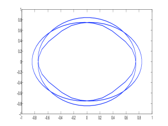
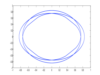
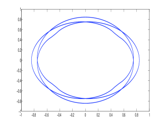
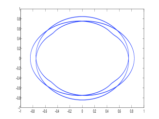
Figure 1: Approximate solution $\omega_{n}(t)$ of the Sherman–Lauricella equation (1.2) on the unit square $\Gamma$ with $f:=f_{1}$ defined by (2.7) and $d=0$. From the left to the right: $n=128,256,512,1024$

Recall that $\mathrm{supp}\,\phi_{nj}\subset[j/n,\;(j+d+1)/n]$ and use the Gauss-Legendre quadrature rule with quadrature points which coincide with the zeros of the Legendre polynomial $P_{24}(x)$ on the canonical interval $[-1,1]$, scaled and shifted to the interval $[j/n,\;(j+d+1)/n]$. More specifically, the corresponding formula is

$$(B_{\Gamma}\omega_{n},\phi_{nj})=\int_{j/n}^{(j+d+1)/n}B_{\Gamma}\omega_{n}(\phi(s))\overline{\phi_{nj}(\phi(s))}ds\approx\sum_{k=1}^{24}w_{k}B_{\Gamma}\omega_{n}(\phi(s_{k}))\phi_{nj}(\phi(s_{k})),$$ (2.9)

where $w_{k},\,s_{k}$ are the Gauss-Legendre weights and the Gauss-Legendre points on the interval $[j/n,\;(j+d+1)/n]$. In order to find the values of the corresponding line integrals at the Gauss-Legendre points, the composite Gauss-Legendre quadrature is used [7, Section 3], namely,

$$\int_{\Gamma}k(t,\tau)x(\tau)d\tau =\int_{0}^{1}k(\gamma(\sigma),\gamma(s))x(\gamma(s))\gamma^{\prime}(s)ds$$ (2.10)

$$\approx\sum_{l=0}^{m-1}\sum\limits_{p=0}^{r-1}w_{p}k(\gamma(\sigma),\gamma(s_{lp}))x(\gamma(s_{lp}))\tau^{\prime}_{lp}/m,$$

where $\tau^{\prime}_{lp}=\gamma^{\prime}(s_{lp})$ with $m=40$ and $r=24$.

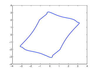
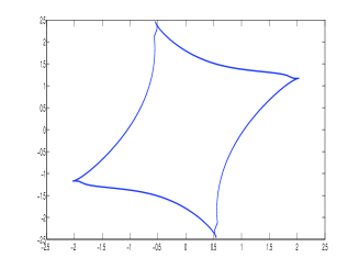
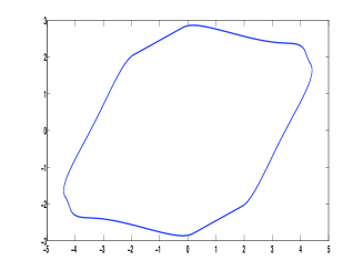
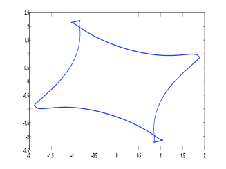
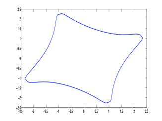
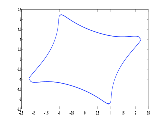
Figure 2: Approximate solution $\omega_{n}(t)$ of the Sherman–Lauricella equation (1.2) on the rhombus $\Gamma$, $\alpha=\pi/3$ with $f:=f_{1}$ defined by (2.7) and $d=0$. From the left to the right: $n=128,256,512,1024$

Figure 3: Approximate solution $\omega_{n}(t)$ of the Sherman–Lauricella equation (1.2) on the rhombus $\Gamma$, $\alpha=\pi/4$ with $f:=f_{1}$ defined by (2.7) and $d=0$. From the left to the right: $n=128,256,512,1024$

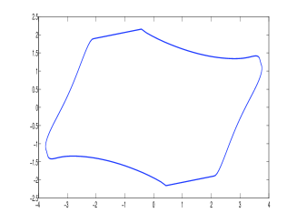
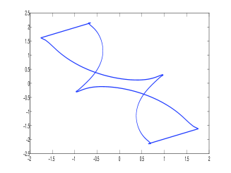
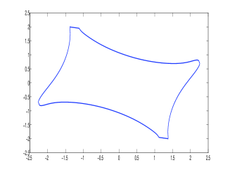
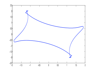
Figure 4: Approximate solution $\omega_{n}(t)$ of the Sherman–Lauricella equation (1.2) on the rhombus $\Gamma$, $\alpha=\pi/5$ with $f:=f_{1}$ defined by (2.7) and $d=0$. From the left to the right: $n=128,256,512,1024$

Table 1 and Figures 1-3 show a good convergence of approximate solutions if the corner point of the contour has an opening angle close or equal to $\pi/2$. On the other hand, the presence of opening angles of a small magnitude can cause problems and lead to a convergence slowdown (see Figures 3-4). Note that although the focus of this work is on the stability, the error estimates presented in Table 1 are comparable with estimates of recent work [16] for fast Fourier–Galerkin method for an integral equation used to solve boundary value problem (1.1) in smooth domains. Moreover, further improvement of the convergence rate is possible if for the approximations of singular integrals and inner products arising in the Galerkin method one employs graded meshes of various kind [2, 15].

3 Galerkin method. Local operators and stability

Our next task is to find conditions of applicability of the spline Galerkin methods to the equation (2.2). It is worth mentioning that for smooth contours $\Gamma$, the methods considered here are always applicable and provide satisfactory results. For details the reader can consult [5], where similar methods for the Muskhelishvili equation on smooth contours are considered. On the other hand, the presence of corners changes the situation drastically, and the applicability of the approximation method is not always guaranteed.

Let $P_{n}$ be the orthogonal projection from $L^{2}(\Gamma)$ on the subspace $S_{n}^{d}(\Gamma)$. Then the systems (2.6) is equivalent to the following operator equations

$$P_{n}B_{\Gamma}P_{n}\omega_{n}=P_{n}f,\quad n\in{\mathbb{N}}.$$ (3.1)

Definition 3.1

We say that the sequence $(P_{n}B_{\Gamma}P_{n})$ is stable if there is an $m\in{\mathbb{R}}$ and an $n_{0}\in{\mathbb{N}}$ such that for all $n\geq n_{0}$ the operators $P_{n}B_{\Gamma}P_{n}:S_{n}^{d}(\Gamma)\to S_{n}^{d}(\Gamma)$ are invertible and

$$||(P_{n}B_{\Gamma}P_{n})^{-1}P_{n}||\leq m$$

for all $n\geq n_{0}$.

Recall that if the stability of the corresponding sequence $(P_{n}B_{\Gamma}P_{n})$ is established, then the convergence of the Galerkin method and error estimates can be obtained from well known results, cf. [11, Section 1.6, inequality (1.30)]. Therefore, in this work we mainly deal with the stability and our approach is based on $C^{*}$-algebra methods often used in operator theory. Let $\mathcal{L}_{add}(L^{2}(\Gamma))$ refer to the real $C^{*}$-algebra of all additive continuous operators on the space $L^{2}(\Gamma)$. One can show [11] that any operator $A\in\mathcal{L}_{add}(L^{2}(\Gamma))$ admits the unique representation $A=A_{1}+A_{2}M$ where $A_{1},A_{2}$ are linear operators and $M$ is the operator of complex conjugation. This representation allows one to introduce the operation of involution on $\mathcal{L}_{add}(L^{2}(\Gamma))$ as follows

$$A^{*}:=A_{1}^{*}+MA_{2}^{*},$$ (3.2)

with $A_{1}^{*},A_{2}^{*}$ being usual adjoint operators to the linear operators $A_{1},A_{2}$, cf. [11, Theorem 1.3.8 and Example 1.3.9]. By $\mathcal{A}^{\Gamma}$ we denote the set of all bounded sequences $(A_{n})$ of bounded additive operators $A_{n}:\mathrm{im}\,P_{n}\to\mathrm{im}\,P_{n}$ such that there is an operator $A\in\mathcal{L}_{add}(L^{2}(\Gamma))$ with the property

$$s-\lim A_{n}P_{n}=A,\quad s-\lim\,(A_{n}P_{n})^{*}P_{n}=A^{*},$$

where $s-\lim A_{n}$ denotes the strong limit of the operator sequence $(A_{n})$.

Provided with natural operations of addition, multiplication, multiplication by scalars $\lambda\in{\mathbb{C}}$, with an involution introduced according to (3.2), and with the norm

$$||(A_{n})||:=\sup_{n\in{\mathbb{N}}}||A_{n}||,$$

the set $\mathcal{A}^{\Gamma}$ becomes a real $C^{*}$-algebra. Consider also the subset $\mathcal{J}^{\Gamma}\subset\mathcal{A}^{\Gamma}$ consisting of all sequences $(J_{n})$ of operators $J_{n}:\mathrm{im}\,P_{n}\to\mathrm{im}\,P_{n}$ which can be represented in the form

$$J_{n}=P_{n}TP_{n}+C_{n},\quad n\in{\mathbb{N}},$$

where the operator $T$ belongs to the ideal $\mathcal{K}_{add}(L^{2}(\Gamma))\subset\mathcal{L}_{add}(L^{2}(\Gamma))$ of all compact operators and the sequence $(C_{n})$ tends to zero uniformly, i.e.

$$\lim_{n\to\infty}||C_{n}||=0.$$

The stability of sequences from the algebra $\mathcal{A}^{\Gamma}$ can be characterized as follows.

Theorem 3.1 (cf. [11, Proposition 1.6.3])

A sequence $(A_{n})\in\mathcal{A}^{\Gamma}$ such that $A:=s-\lim A_{n}P_{n}$ is stable if and only if the operator $A$ is invertible in $\mathcal{L}_{add}(L^{2}(\Gamma))$ and the coset $(A_{n})+\mathcal{J}^{\Gamma}$ is invertible in the quotient algebra $\mathcal{A}^{\Gamma}/\mathcal{J}^{\Gamma}$.

Consider now the sequence $(P_{n}B_{\Gamma}P_{n})$ of the Galerkin operators defined by the projection operators $P_{n}$. Recall that on the space $L^{2}(\Gamma)$ the sequence of the orthogonal projections $(P_{n})$ strongly converges to the identity operator $I$ and $P_{n}^{*}=P_{n},n\in{\mathbb{N}}$. It implies that for any operator $A\in\mathcal{L}_{add}(L^{2}(\Gamma))$ the following relations

$$s-\lim P_{n}AP_{n}=A,\quad s-\lim(P_{n}AP_{n})^{*}P_{n}=A^{*}$$

hold [25]. Therefore, combining Theorem 2.1 and Theorem 3.1 one obtains the following result.

Corollary 3.1

Let $\Gamma$ be a simple closed piecewise smooth curve. The spline Galerkin method (3.1) is stable if and only if the coset $(P_{n}B_{\Gamma}P_{n})+\mathcal{J}^{\Gamma}$ is invertible in the quotient algebra $\mathcal{A}^{\Gamma}/\mathcal{J}^{\Gamma}$.

Thus in order to establish the stability of the Galerkin method, one has to study the invertibility of the coset $(P_{n}B_{\Gamma}P_{n})+\mathcal{J}^{\Gamma}$ in the algebra $\mathcal{A}^{\Gamma}/\mathcal{J}^{\Gamma}$. This problem can be tackled more efficiently, if we restrict ourselves to a smaller algebra containing the coset $(P_{n}B_{\Gamma}P_{n})+\mathcal{J}$. More precisely, let $M$ refer to the operator of the complex conjugation,

$$M\phi(t):=\overline{\phi(t)},\quad t\in\Gamma,$$

and let $S_{\Gamma}$ be the Cauchy singular integral operator,

$$S_{\Gamma}\phi(t):=\frac{1}{\pi i}\int_{\Gamma}\frac{\phi(\zeta)}{\zeta-t}\,d\zeta.$$

Consider the smallest closed real $C^{*}$-subalgebra $\mathcal{B}^{\Gamma}$ of the algebra $\mathcal{A}^{\Gamma}$ which contains all operator sequences of the form $(P_{n}MP_{n}),(P_{n}S_{\Gamma}P_{n})$ and also the sequences $(P_{n}fP_{n}),f\in{\mathbb{C}}_{\mathbb{R}}(\Gamma)$ and $(G_{n})$, where $\lim_{n\to\infty}||G_{n}||=0$ and ${\mathbb{C}}_{\mathbb{R}}(\Gamma)$ is the set of all continuous real-valued functions on the contour $\Gamma$.

Remark 3.1

It follows from [10, 12, 21, 25] that $\mathcal{J}^{\Gamma}\subset\mathcal{B}^{\Gamma}$ and that the sequence $(P_{n}B_{\Gamma}P_{n})$ belongs to $\mathcal{B}^{\Gamma}$. Therefore, $\mathcal{B}^{\Gamma}/\mathcal{J}^{\Gamma}$ is a real $C^{*}$-subalgebra of $\mathcal{A}^{\Gamma}/\mathcal{J}^{\Gamma}$, and by [11, Corollary 1.4.10] the coset $(P_{n}B_{\Gamma}P_{n})+\mathcal{J}^{\Gamma}$ is invertible in $\mathcal{A}^{\Gamma}/\mathcal{J}^{\Gamma}$ if and only if it is invertible in $\mathcal{B}^{\Gamma}/\mathcal{J}^{\Gamma}$. Therefore, one can now study the invertibility of the coset $(P_{n}B_{\Gamma}P_{n})+\mathcal{J}^{\Gamma}$ in the smaller algebra $\mathcal{B}^{\Gamma}/\mathcal{J}^{\Gamma}$. To this end we will employ a localizing principle.

Thus with each point $\tau\in\Gamma$ we associate a model contour $\Gamma_{\tau}$ as follows. Let $\theta_{\tau}$ be the angle between the right and the left semi-tangents to $\Gamma$ at the point $\tau$, and let $\beta_{\tau}$ refer to the angle between the right semi-tangent to $\Gamma$ and the real line ${\mathbb{R}}$. Consider now the curve

$$\Gamma_{\tau}:=e^{i(\beta_{\tau}+\theta_{\tau})}{\mathbb{R}}_{+}^{-}\cup e^{i\beta_{\tau}}{\mathbb{R}}_{+}^{+}$$

where ${\mathbb{R}}_{-}^{+}$ and ${\mathbb{R}}_{+}^{+}$ denote the positive semi-axis ${\mathbb{R}}^{+}$ correspondingly directed to and out of the origin. Further, on each such contour $\Gamma_{\tau}$, $\tau\in\Gamma$ we consider the corresponding Sherman-Lauricella operator

$$A_{\tau}=I+L_{\tau}-K_{\tau}M,$$ (3.3)

where

$$L_{\tau}\omega(t):=\frac{1}{2\pi i}\int_{\Gamma_{\tau}}\omega(\zeta)\,d\ln\left(\frac{\zeta-t}{{\overline{\zeta}}-{\overline{t}}}\right),\quad K_{\tau}\omega(t):=\frac{1}{2\pi i}\int_{\Gamma_{\tau}}\omega(\zeta)\,d\left(\frac{{\overline{\zeta}}-{\overline{t}}}{\zeta-t}\right).$$

Analogously to the algebra $\mathcal{B}^{\Gamma}$ and to the ideal $\mathcal{J}^{\Gamma}$ one can introduce algebras $\mathcal{B}^{\Gamma_{\tau}}$ and ideals $\mathcal{J}^{\Gamma_{\tau}}\subset\mathcal{B}^{\Gamma_{\tau}}$, $\tau\in\Gamma$, which allow to establish conditions of the applicability of the corresponding Galerkin method for the operators (3.3). For this we also need appropriate spline spaces on both the contour $\Gamma_{\tau}$ and the positive semi-axis ${\mathbb{R}}^{+}:={\mathbb{R}}^{+}_{+}$. These spline spaces can be constructed by using the functions (2.4) again. More precisely, consider the functions

$$\widetilde{\phi}_{nj}(t):=\left\{\begin{array}[]{l}\left\{\begin{array}[]{cc}\phi_{nj}(s)&\displaystyle\text{if}\quad t=e^{i\beta_{\tau}}s\\ 0&\text{otherwise}\\ \end{array}\right.\quad j\geq 0\\[12.91663pt] \left\{\begin{array}[]{cc}\phi_{n,j-d}(s)&\displaystyle\text{if}\quad t=e^{i(\beta_{\tau}+\theta_{\tau})}s\\ 0&\text{otherwise}\\ \end{array}\right.\quad j<0\end{array}.\right.$$ (3.4)

Let $S_{n}^{d}(\Gamma_{\tau})$ and $S_{n}^{d}({\mathbb{R}}^{+})$ be, respectively, the smallest closed subspaces of $L_{2}(\Gamma_{\tau})$ and $L^{2}({\mathbb{R}}^{+})$ which contains all functions (3.4) and all functions $\phi_{nj}$, $j\geq 0$ of (3.4) for $\beta_{\tau}=0$. Moreover, let $P_{n}^{\tau}$, $n\in{\mathbb{N}}$ and $P_{n}^{+}$ denote the orthogonal projection onto subspaces $S_{n}^{d}(\Gamma_{\tau})$ and $S_{n}^{d}({\mathbb{R}}^{+})$, respectively. In order to study the stability of the sequence $(P_{n}^{\tau}A_{\tau}P_{n}^{\tau})$, one can apply Theorem 3.1 and Remark 3.1 to obtain the following result.

Corollary 3.2

The sequence $(P_{n}^{\tau}A_{\tau}P_{n}^{\tau})\in\mathcal{B}^{\Gamma_{\tau}}$ is stable if and only if the operator $A_{\tau}$ is invertible in $\mathcal{B}^{\tau}$ and the coset $(P_{n}^{\tau}A_{\tau}P_{n}^{\tau})+\mathcal{J}^{\Gamma_{\tau}}$ is invertible in the quotient algebra $\mathcal{B}^{\Gamma_{\tau}}/\mathcal{J}^{\Gamma_{\tau}}$.

Further, let $L^{2}_{2}({\mathbb{R}}^{+})$ be the space of all pairs $(\varphi_{1},\varphi_{2})^{T},\,\varphi_{1},\varphi_{2}\in L^{2}({\mathbb{R}}^{+})$ provided with the norm

$$||(\varphi_{1},\varphi_{2})^{T}||:=\left(\right||\varphi_{1}||^{2}+||\varphi_{2}||^{2})^{1/2},$$

and let $\eta:L^{2}(\Gamma_{\tau})\to L^{2}_{2}({\mathbb{R}}^{+})$ be the mapping defined by

$$\eta(\varphi)=(\varphi(se^{i(\beta_{\tau}+\omega_{\tau})}),\varphi(se^{i\beta}))^{T},\quad s\in\mathbb{R}^{+},$$

where $a^{T}$ denotes the transposition of the vector $a$. It is clear that $\eta$ is a linear isometry from $L^{2}(\Gamma_{\tau})$ onto $L^{2}_{2}({\mathbb{R}}^{+})$. Moreover, the mapping $\Psi:\mathcal{L}_{add}(L^{2}(\Gamma_{\tau}))\to\mathcal{L}_{add}(L^{2}_{2}({\mathbb{R}}^{+}))$ defined by

$$\Psi(A)=\eta A\eta^{-1},$$ (3.5)

is an isometric algebra isomorphism. In particular, straightforward calculations show that

$$\Psi(P_{n}^{\tau}) =\mathrm{diag}\,(P_{n}^{+},P_{n}^{+}),$$ (3.6)

$$\Psi(M) =\mathrm{diag}\,(\widetilde{M},\widetilde{M}),$$ (3.7)

$$\Psi(L_{\tau}) =\left(\begin{array}[]{cc}0&\mathcal{N}_{\theta_{\tau}}\\[4.30554pt] \mathcal{N}_{\theta_{\tau}}&0\\ \end{array}\right),$$ (3.10)

$$\Psi(K_{\tau}) =\left(\begin{array}[]{cc}0&e^{i2\beta_{\tau}}\mathcal{M}_{2\pi-\theta_{\tau}}\\[4.30554pt] -e^{i2(\beta_{\tau}+\theta_{\tau})}\mathcal{M}_{\theta_{j}}&0\\ \end{array}\right),$$ (3.13)

where

$$\mathcal{N}_{\theta_{\tau}}\varphi(\sigma)=\frac{1}{2}\frac{1}{2\pi i}\int_{0}^{\infty}\left(\frac{1}{1-(\sigma/s)e^{i\theta_{\tau}}}-\frac{1}{1-(\sigma/s)e^{i(2\pi-\theta_{\tau})}}\right)\varphi(s)\frac{ds}{s},$$

$$\mathcal{M}_{\theta_{\tau}}\varphi(\sigma):=\frac{1}{\pi}\int_{0}^{\infty}\left(\frac{\sigma}{s}\right)\frac{\sin\theta_{\tau}}{(1-(\sigma/s)e^{i\theta_{\tau}})^{2}}\varphi(s)\frac{ds}{s},$$

and the symbol $\widetilde{M}$ in the right-hand side of (3.7) refers to the operator of the complex conjugation on the space $L^{2}({\mathbb{R}}^{+})$. Moreover, one can observe that the operators $\mathcal{N}_{\theta_{\tau}}$ and $\mathcal{M}_{\theta_{\tau}}$ have a special form – viz.

$$K\varphi(\sigma):=\int_{0}^{\infty}\mathsf{k}_{\theta_{\tau}}\left(\frac{\sigma}{s}\right)\varphi(s)\frac{ds}{s}$$ (3.14)

and

$$\mathsf{k}_{\theta_{\tau}}=\mathsf{k}_{\theta_{\tau}}(u) :=\mathsf{n}_{\theta_{\tau}}(u)=\frac{1}{2\pi}\frac{u\sin\theta_{\tau}}{|1-ue^{i\theta_{\tau}}|^{2}},\quad\text{if}\quad K=\mathcal{N}_{\theta_{\tau}},$$ (3.15)

$$\mathsf{k}_{\theta_{\tau}}=\mathsf{k}_{\theta_{\tau}}(u) :=\mathsf{m}_{\theta_{\tau}}(u)=\frac{1}{\pi}\frac{u\sin\theta_{\tau}}{(1-ue^{i\theta_{\tau}})^{2}},\quad\text{if}\quad K=\mathcal{M}_{\theta_{\tau}}.$$ (3.16)

On the space $l^{2}$ of the sequences $(\xi_{k})$ of complex numbers $\xi_{k},k=0,1,\ldots$,

$$l^{2}:=\{(\xi_{k})_{k=0}^{\infty}:\sum_{k=0}^{\infty}|\xi_{k}|^{2}<\infty\},$$

the function $\textsf{k}_{\theta_{\tau}}$ defines a bounded linear operator $A(\mathsf{k}_{\theta_{\tau}})$ with the matrix representation

$$A(\mathsf{k}_{\theta_{\tau}})=\left(\nu_{d}^{2}\int_{0}^{d+1}\widehat{\phi}(t)\int_{0}^{d+1}\mathsf{k}_{\theta_{\tau}}\left(\frac{u+l}{t+q}\right)\widehat{\phi}(u)\frac{du}{u+q}\,dt\right)_{q,l=0}^{\infty}\,,$$

where $\nu_{d}$ is the constant (2.3).

Theorem 3.2

Let $\mathsf{n_{\theta_{\tau}}}$ and $\mathsf{m_{\theta_{\tau}}}$ be the functions defined by (3.15) and (3.16), respectively. The spline Galerkin method (3.1) is stable if and only if the operators $R^{\tau}:l^{2}\times l^{2}\to l^{2}\times l^{2}$,

$$R^{\tau}:=$$ (3.17)

$$\left(\begin{array}[]{c@{\hspace{-1mm}}c}I&A(\mathsf{n}_{\theta_{\tau}})\\[4.30554pt] A(\mathsf{n}_{\theta_{\tau}})&I\\ \end{array}\right)\!\!+\!\!\left(\begin{array}[]{c@{\hspace{-1mm}}c}0&e^{i\beta_{\tau}}A(\mathsf{m}_{2\pi-\theta_{\tau}})\\[4.30554pt] -e^{-i(\beta_{\tau}+\theta_{\tau})}A(\mathsf{m}_{\theta_{\tau}})&0\\ \end{array}\right)\left(\begin{array}[]{cc}\overline{M}&0\\[4.30554pt] 0&\overline{M}\\ \end{array}\right)$$

are invertible for all $\tau\in\mathcal{M}_{\Gamma}$.

Proof. By Corollary 3.1 the sequence $(P_{n}B_{\Gamma}P_{n})$ is stable if and only if the coset $(P_{n}B_{\Gamma}P_{n})+\mathcal{J}^{\Gamma}$ is invertible. Moreover, since $T_{\Gamma}$ of (2.1) is a compact operator, the sequences $(P_{n}A_{\Gamma}P_{n})$ and $(P_{n}B_{\Gamma}P_{n})$ belong to the same coset $(P_{n}A_{\Gamma}P_{n})+\mathcal{J}^{\Gamma}$ of the quotient algebra $\mathcal{B}^{\Gamma}/\mathcal{J}^{\Gamma}$. However, by a version of the Allan’s Local Principle [1] for real $C^{*}$-algebras [11, Theorem 1.9.5], the coset $(P_{n}A_{\Gamma}P_{n})+\mathcal{J}^{\Gamma}$ is invertible if and only if for every $\tau\in\Gamma$ the coset $(P_{n}^{\tau}A_{\Gamma_{\tau}}P_{n}^{\tau})+\mathcal{J}^{\Gamma_{\tau}}$ is invertible in the corresponding algebra $\mathcal{B}^{\Gamma_{\tau}}/\mathcal{J}^{\Gamma_{\tau}}$. Therefore, the stability of our operator sequence will be established if we manage to show the invertibility of all cosets $(P_{n}^{\tau}A_{\Gamma_{\tau}}P_{n}^{\tau})+\mathcal{J}^{\Gamma_{\tau}}$, $\tau\in\Gamma$. Let us start with the case where $\tau$ is not a corner point of $\Gamma$. If $\tau\notin\mathcal{M}_{\Gamma}$, then $\theta_{\tau}=\pi$, and straightforward calculations show that $L_{\tau}$ and $K_{\tau}$ are the zero operators. Hence, $A_{\tau}$ is just the identity operator $I$ in the corresponding space, so that $P_{n}^{\tau}A_{\tau}P_{n}^{\tau}=P_{n}^{\tau}$. The sequence $(P_{n}^{\tau})$ is obviously stable so that the corresponding coset $(P_{n}^{\tau})+\mathcal{J}^{\tau}$ is invertible.

Consider next the case where $\tau\in\mathcal{M}_{\Gamma}$. Note that by [7, Theorem 2.2] the operator $A_{\tau}$ is invertible on the space $L^{2}(\Gamma)$. Therefore, by Corollary 3.2 the coset $(P_{n}^{\tau}A_{\tau}P_{n}^{\tau})+\mathcal{J}^{\tau}$ is invertible in $\mathcal{B}^{\Gamma_{\tau}}/\mathcal{J}^{\Gamma_{\tau}}$ if and only if the sequence $(P_{n}^{\tau}A_{\tau}P_{n}^{\tau})$ is stable. However, the stability of this sequence is equivalent to the stability of the sequence $(\Psi(P_{n}^{\tau}A_{\tau}P_{n}^{\tau}))$, where mapping $\Psi$ is defined by (3.5). Consider also the operators $\Lambda_{n}:S_{n}^{d}({\mathbb{R}}^{+})\to l^{2}$ defined by

$$\Lambda_{n}\left(\sum_{j=0}^{\infty}\xi_{j}\phi_{nj}\right)=(\xi_{0},\xi_{1},\ldots,\,).$$

By Lemma 2.1 these operators are bounded and continuously invertible. Set $\Lambda_{-n}:=\Lambda_{n}^{-1}$ and note that the sequence $(\Psi(P_{n}^{\tau}A_{\tau}P_{n}^{\tau}))$ is stable if and only if so is the sequence $(R_{n}^{\tau})$, where

$$R_{n}^{\tau}=\mathrm{diag}\,(\Lambda_{n},\Lambda_{n})\cdot\Psi(P_{n}^{\tau}A_{\tau}P_{n}^{\tau})\cdot\mathrm{diag}\,(\Lambda_{-n},\Lambda_{-n}):l^{2}\times l^{2}\to l^{2}\times l^{2}.$$

From the definition of the mappings $\Psi$ and $\Lambda_{\pm n}$ one obtains that the operators $R_{n}^{\tau}$ have the form

$$R_{n}^{\tau}=(A_{lp}^{(n,\tau)})_{l,p=1}^{2}+(B_{lp}^{(n,\tau)})_{l,p=1}^{2}\mathrm{diag}\,(\overline{M},\overline{M}),$$

with the operators $A_{lp}^{(n,\tau)},B_{lp}^{(n,\tau)}:l^{2}\to l^{2}$ defined according to the relations (3.6)-(3.13). However, these operators do not depend on the parameter $n$ at all. Really, consider the matrix representations of the operators $A_{12}^{(n,\tau)},A_{21}^{(n,\tau)},B_{12}^{(n,\tau)},B_{21}^{(n,\tau)}$. It follows from (3.14) that the entries $a_{lq}$ of the corresponding matrices $(a_{lq})_{l,q=0}^{\infty}$ are

$$a_{pq} =\int_{{\mathbb{R}}^{+}}K\phi_{qn}(\sigma)\phi_{ln}(\sigma)\,d\sigma=\int_{{\mathbb{R}}^{+}}\int_{{\mathbb{R}}^{+}}\mathsf{k}_{\theta_{\tau}}\left(\frac{\sigma}{s}\right)\phi(ns-q)\frac{ds}{s}\phi(n\sigma-l)\,d\sigma$$

$$=\frac{1}{n}\int_{{\mathbb{R}}^{+}}\int_{{\mathbb{R}}^{+}}\mathsf{k}_{\theta_{\tau}}\left(\frac{u+l}{t+q}\right)\phi(u)\frac{du}{u+q}\phi(t)\,dt$$

$$=\frac{1}{n}\int_{{\mathbb{R}}^{+}}\int_{{\mathbb{R}}^{+}}\mathsf{k}_{\theta_{\tau}}\left(\frac{u+l}{t+q}\right)(\nu_{d}\sqrt{n}\widehat{\phi}(u))\frac{du}{u+q}(\nu_{d}\sqrt{n}\widehat{\phi}(t))\,dt$$

$$=\nu_{d}^{2}\int_{0}^{d+1}\widehat{\phi}(t)\int_{0}^{d+1}\mathsf{k}_{\theta_{\tau}}\left(\frac{u+l}{t+q}\right)\widehat{\phi}(u)\frac{du}{u+q}\,dt,$$

hence these operators are independent of $n$. Moreover, $B_{11}^{(n,\tau)},B_{22}^{(n,\tau)}=0$ and $A_{11}^{(n,\tau)}=A_{22}^{(n,\tau)}=I$. Combining all the above representations, one obtains that the operators $R_{n}^{\tau}$ do not depend on the parameter $n$. Therefore, $(R_{n}^{\tau})$ is a constant sequence and it is stable if and only if any its member, say $R^{\tau}_{1}$, is invertible. It remains to observe that $R^{\tau}=R^{\tau}_{1}$, which completes the proof.  

4 Numerical approach to the invertibility of local operators

.

As was already mentioned, there is no efficient analytic method to verify the invertibility of the local operators $R^{\tau}$. On the other hand, numerical approaches turn out to be surprisingly fruitful. Recall that the operators $R^{\tau},\;\tau\in\mathcal{M}_{\Gamma}$ do not depend on the shape of the contour $\Gamma$ but only on the relevant angles $\theta_{\tau}$ and $\beta_{\tau}$. Therefore, for contours having only one corner point, Theorem 3.2 can be reformulated as follows.

Corollary 4.1

If $\tau$ is the only corner point of the contour $\Gamma$, then the operator $R^{\tau}$ is invertible if and only if the Galerkin method $(P_{n}B_{\Gamma}P_{n})$ is stable.

Thus in order to determine the critical angles, i.e. the opening angles $\theta$ for which the operators $R^{\tau}$ are not invertible, one can consider the behaviour of the spline Galerkin methods on special contours. A family of such contours $\Gamma_{1}^{\theta}$, $\theta\in(0,2\pi)$,

$$\Gamma_{1}^{\theta}:=\{t\in{\mathbb{C}}:t=\gamma_{1}(s)=\sin(\pi s)\exp(i\theta(s-0.5)),\;s\in[0,1]\}$$

has been used in [6, 9] to study the local operators of the Nyström method for Sherman–Lauricella and Muskhelishvili equations. Changing the parameter $\theta$ in the interval $(0,2\pi)$, one obtains contours located at the origin and having only one corner of various magnitude. In the present paper, we use the same contours to detect the critical angles of the spline Galerkin methods. It is worth mentioning that the operator $R^{\tau}$ depends not only on $\theta_{\tau}$ but also on the angle $\beta_{\tau}$ between the right semi-tangent to the contour $\Gamma_{1}^{\theta}$ at the point $\tau$ and the real line ${\mathbb{R}}$. However, numerical experiments conducted for both the Nyström and spline Galerkin methods show that, in fact, the angle $\beta_{\tau}$ does not influence the invertibility of the operator $R^{\tau}$. This opens a way for verifying the results obtained for contour $\Gamma_{1}^{\theta}$ by conducting similar tests for equations on contours with two or more corner, all of the same magnitude. To this end, we will use another contour $\Gamma_{2}^{\theta}$, which is the union of two circular arcs with the parametrization

$$\displaystyle\gamma_{1}(s) =-0.5\cot(0.5\theta)+0.5/\sin(0.5\theta)\,\exp(i\theta(s-0.5)),\quad 0\leq s\leq 1,$$

$$\displaystyle\gamma_{2}(s) =\phantom{-}0.5\cot(0.5\theta)-0.5/\sin(0.5\theta)\,\exp(i\theta(s-0.5)),\quad 0\leq s\leq 1.$$

To find the angles of instability, the interval $[0.1\pi,\;1.9\pi]$ has been divided by the points $\theta_{k}:=\pi(0.1+0.01k)$ and for each opening angle $\theta_{k}$ we constructed the matrices of the corresponding approximation operators for the Galerkin methods based on the splines of degree $d=0,d=1$ and $d=2$.

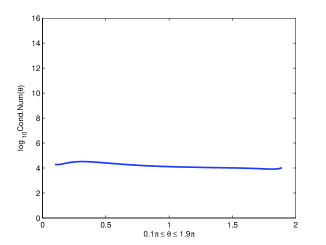
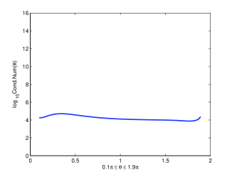
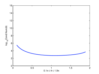
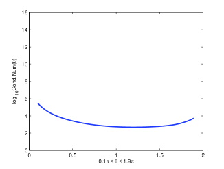
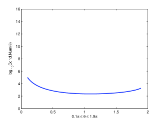
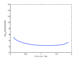
Figure 5: Condition numbers vs. opening angles in case $n=128$. From row 1 to row 3: splines of degree 0, 1 and 2, respectively. Left column: one-corner geometry, right column: two-corner geometry.

Note that we consider Galerkin methods for two choices of $n$, namely for $n=128$ and $n=256$, and the integrals arising in the equation (2.2) and in the method (2.6) have been approximated by quadrature formulas (2.9), (2.10). Further, to verify the stability of the method, for each angle $\theta_{k}$ we compute the condition numbers of the corresponding matrices and the results of these computations are presented in Figures 5-7, where possible presence of peaks might indicate critical angles. Thus it seems that inside of the interval $(0.1\pi,1.9\pi)$ neither of the Galerkin methods based on splines of degree $0,1$ or $2$ has critical angles. This differs from the Nyström method, where critical angles have been discovered for both Sherman–Lauricella and Muskhelishvili equations [6, 9]. Contrariwise, information about the critical angles at the interval ends is not so conclusive. Thus in the case $n=256$, the computation of the condition numbers for both one and two corner geometry shows that for the Galerkin method based on the splines of degree zero there can be a critical angle at the right end of the interval mentioned.

For splines of the degree $d=0$ and $d=1$, the one and two corner geometries give contradictory results (see Figure 6).

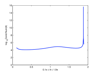
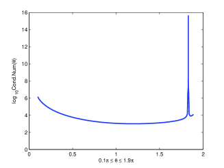
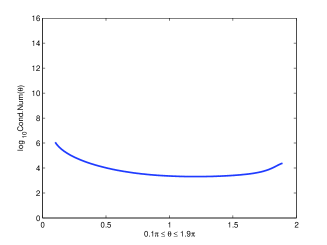
Figure 6: Condition numbers vs. opening angles in case $n=256$. From row 1 to row 3: splines of degree 0, 1 and 2, respectively. Left column: one-corner geometry, right column: two-corner geometry.

To clarify the situation one has to refine the mesh $\{\theta_{k}\}$ and essentially increase the dimension of the matrices used. Note that while discovering a suspicious critical angle for $n=256$, we refined the mesh $\{\theta_{k}\}$ in a neighbourhood of that angle by reducing its step to $0.001\pi$, and calculated the condition numbers for the corresponding Galerkin methods with $n$ changed to $512$. This allows us to show that, in fact, there are no critical angles in the interval mentioned. However, the computing time increases drastically.

The numerical experiments are performed in MATLAB environment (version 7.9.0) and executed on an Acer Veriton M680 workstation equipped with a Intel Core i7 vPro 870 Processor and 8GB of RAM, and it took from one to two weeks of computer work in order to obtain every single graph presented in Figure 5, 6 or 7.

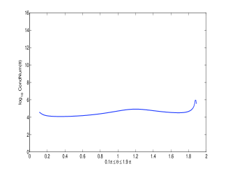
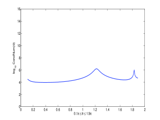
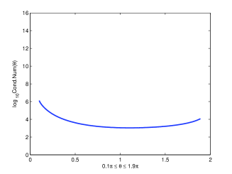
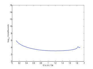
Figure 7: Condition numbers vs. opening angles in case $n=256$ and $n=512$ in neighbourhoods of suspicious points. From row 1 to row 3: splines of degree 0, 1 and 2, respectively. Left column: one-corner geometry, right column: two-corner geometry.

References

[1]G. R. Allan, Ideals of vector-valued functions, Proc.
London
Math. Soc., 18 (1968), pp. 193–216.
[2]Q. Chen, T. Tang, and Z. Teng, A fast numerical method
for integral equations of the first kind with logarithmic kernel using mesh
grading, J. Comput. Math., 22 (2004), pp. 287–298.
.
[3]D. Crowdy, Exact solutions for the viscous sintering of
multiply-connected fluid domains, J. Engrg. Math., 42 (2002), pp. 225–242.
[4]C. De Boor, A practical guide to splines, Springer
Verlag,
New-York-Heidelberg-Berlin, 1978.
[5]V. Didenko and E. Venturino, Approximation methods for
the
Muskhelishvili equation on smooth curves, Math. Comp., 76 (2007),
pp. 1317–1339 (electronic).
[6]V. D. Didenko and J. Helsing, Features of the
Nyström method
for the Sherman-Lauricella equation on piecewise smooth contours, East
Asian J. Appl. Math., 1 (2011), pp. 403–414.
[7]V.D. Didenko and J. Helsing, Stability of the Nyström
method for the Sherman-Lauricella equation, SIAM J. Numer. Anal., 49
(2011), pp. 1127–1148.
[8]V.D. Didenko and J. Helsing, Approximate solution
of boundary integral equations for biharmonic problems in non-smooth
domains, Proc. Appl. Math. Mech., 13 (2013), pp. 435–438.
[9]V.D. Didenko and J. Helsing, On the stability of
the Nyström method for the Muskhelishvili equation on contours with
corners, SIAM J. Numer. Anal., 51 (2013), pp. 1757–1776.
[10]V.D. Didenko and B. Silbermann, On stability of
approximation
methods for the Muskhelishvili equation, J. Comput. Appl. Math., 146
(2002), pp. 419–441.
[11]V.D. Didenko and B. Silbermann, Approximation of additive
convolution-like operators, Frontiers in Mathematics, Birkhäuser Verlag,
Basel, 2008.
Real -algebra approach.
[12]R.V. Duduchava, Integral equations in convolution with
discontinuous presymbols, singular integral equations with fixed
singularities, and their applications to some problems of mechanics, BSB B.
G. Teubner Verlagsgesellschaft, Leipzig, 1979.
[13]R. V. Duduchava, General singular integral equations and
fundamental
problems of the plane theory of elasticity, Trudy Tbiliss. Mat. Inst.
Razmadze Akad. Nauk Gruzin. SSR, 82 (1986), pp. 45–89.
[14]L. Greengard, M.C.A. Kropinski, and A. Mayo, Integral
equation methods for Stokes flow and isotropic elasticity in the plane, J.
Comput. Phys., 125 (1996), pp. 403–414.
[15]J. Helsing, A fast and stable solver for singular
integral equations
on piecewise smooth curves, SIAM Journal on Scientific Computing, 33 (2011),
pp. 153–174.
[16]Y. Jiang, B. Wang, and Y. Xu, A Fast
Fourier–Galerkin
Method Solving a Boundary Integral Equation for the Biharmonic
Equation, SIAM J. Numer. Anal., 52 (2014), pp. 2530–2554.
[17]A. I. Kalandiya, Mathematical methods of two-dimensional
elasticity, Mir Publishers, Moscow, 1975.
[18]M. C. A. Kropinski, An efficient numerical method for
studying interfacial motion in two-dimensional creeping flows, J.
Comput. Phys., 171
(2001), pp. 479–508.
[19]G. Lauricella, Sur l’intégration de l’équation
relative
à l’équilibre des plaques élastiques encastrées, Acta Math., 32
(1909), pp. 201–256.
[20]S. G. Mikhlin, Integral equations and their applications
to certain
problems in mechanics, mathematical physics and technology, 2nd
edition. Pergamon Press, New York, 1964.
[21]S. G. Mikhlin and S. Prössdorf, Singular integral
operators, Springer-Verlag, Berlin, 1986.
[22]N. I. Muskhelishvili, Fundamental problems in the theory
of elasticity, Nauka, Moscow, 1966.
[23]H. Ockendon and J. R. Ockendon, Viscous flow, Cambridge
Texts in Applied Mathematics, Cambridge University Press,
Cambridge, 1995.
[24]V. Z. Parton and P. I. Perlin, Integral equations in
elasticity,
“Mir”, Moscow, 1982.
[25]S. Prössdorf and B. Silbermann, Numerical analysis for
integral and related operator equations, Birkhäuser Verlag,
Berlin–Basel, 1991.
[27]D. I. Sherman, On the solution of the plane static
problem of the theory of elasticity for given external forces,
Doklady AN SSSR, 28 (1940),
pp. 25–28.