Single and double polarization observables in timelike Compton scattering off proton

Timelike Compton scattering off the proton and Generalized Parton Distributions.

Abstract

We study the exclusive photoproduction of a lepton pair off the proton with the aim of studying the proton quark structure via the Generalized Parton Distributions (GPD) formalism. After deriving the amplitudes of the processes contributing to the $\gamma P\to P^{\prime}e^{+}e^{-}$, the Timelike Compton Scattering and the Bethe-Heitler process, we calculate all unpolarized, single- and double- beam-target spin observables in the valence region in terms of GPDs.

I Introduction

The scattering of light on matter, which can generically be called Compton scattering, is a powerful tool to investigate its inner structure. Nowadays, understanding the structure of hadrons in terms of quark and gluon (partons) degrees of freedom, i.e. the basic constituents of matter known to this day, is the subject of an intense research effort. Only these past fifteen years or so, thanks to the emergence of high intensity, high energy (multi-GeV) and high duty-cycle lepton accelerators, Compton scattering at the partonic level starts to be investigated experimentally in an efficient way.

A particular case of Compton scattering at the partonic level is the Deeply Virtual Compton Scattering (DVCS) process on the proton $P$, i.e. $\gamma^{*}P\to\gamma P^{\prime}$ where the initial virtual photon $\gamma^{*}$ is radiated from an incoming lepton beam (see Fig. 1-top). It is of particular interest as the amplitude of the process allows to access some essential operators of Quantum Chromo-Dynamics (QCD, the fundamental theory governing the interactions of quarks and gluons). Indeed, at sufficiently large virtuality of the initial photon ($Q^{2}=(k-k^{\prime})^{2}$), the DVCS amplitude can be factorized into an elementary “hard” (perturbative) scattering process $\gamma^{*}q\to\gamma q$ (where $q$ is a quark of the proton), exactly calculable from Quantum Electro-Dynamics as well as perturbative QCD, and a “soft” (non-perturbative) QCD bilocal matrix elements. The Fourier transforms into momentum space of these QCD matrix elements are the so-called Generalized Parton Distributions (GPDs). In DVCS on the nucleon, at QCD leading-twist order there are four quark helicity conserving GPDs ($H$, $E$, $\tilde{H}$ and $\tilde{E}$) which can be accessed and which correspond to the four independent helicity-spin transitions between the initial quark-proton system and the final one. The GPDs contain a wealth of information on the partonic structure of the proton: the longitudinal momentum and transverse space distributions of the quarks and gluons, the correlation between these momentum and space distributions, sensitivity to the quark-antiquark content in the proton, the quark orbital momentum contribution to the proton spin, etc… We refer the reader to the reviews goeke ; revdiehl ; revrady ; rpp on GPDs for the details of the formalism and of their properties.

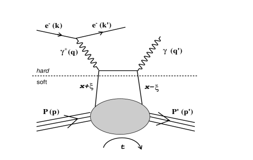
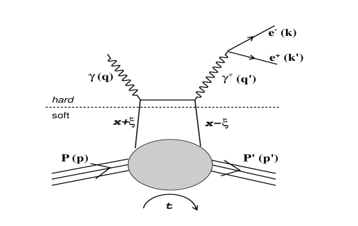
Figure 1: Top: QCD leading-twist DVCS diagram; Bottom: QCD leading-twist TCS diagram (the crossed diagrams of both processes are not shown). The dashed line illustrates the factorization between

DVCS is currently widely investigated, experimentally as well as theoretically. Ref. rpp compiles all existing data in the valence region and presents some first informations on the partonic structure of the proton that can be extracted, within some approximations, from the first DVCS data through the GPD formalism. One example of a pioneering result is the first quantitative evaluation of the increase of the transverse size of the proton as smaller longitudinal momentum fractions of partons are probed.

However, the GPD information is difficult to extract: DVCS cross sections are small (of the order of pb), there is the competing Bethe-Heitler (BH) process which leads to the same final state $eP\gamma$ but where the final photon is emitted from the incoming or scattered lepton and which is therefore not related to GPDs but nevertheless interferes. Furthermore, there is the need of measuring a series of spin (beam and/or target) observables to constrain the different GPDs, etc… It would therefore be useful to investigate if supplementary and/or complementary constraints on GPDs could be obtained from processes other than DVCS. In this spirit, we investigate in this article the related process of Timelike Compton Scattering (TCS) which corresponds to the exclusive photoproduction of a lepton pair on the proton: $\gamma P\to P^{\prime}\gamma^{*}\hookrightarrow e^{+}e^{-}$ and which is displayed in Fig. 1-bottom. Like for DVCS, at sufficiently large virtuality of the final virtual photon ($Q^{\prime 2}=(k+k^{\prime})^{2}$), it is predicted that the process factorizes and is sensitive to GPDs, the same ones accessed in DVCS.

The TCS process was originally investigated in terms of GPDs about ten years ago in Ref. Berger:2001xd . In this pioneering work, analytical formulas in terms of GPDs were derived for the unpolarized and the circularly polarized beam cross sections of the process $\gamma P\to P^{\prime}e^{+}e^{-}$, i.e. on a proton target. Very recently, a second article continued the investigation by studying the linearly polarized beam cross section Goritschnig .

However, in order to obtain simple analytical expressions, a few approximations were used in the calculation of the TCS amplitude (for instance mass correction terms of the order of ${m^{2}}/{Q^{\prime 2}}$ where $m$ is the mass of the proton were neglected). In the present work, we waive some of these approximations and present calculations of different observables. In addition, besides unpolarized cross sections, we study all single and double beam-target spin observables. We focus in this article on a proton target.

This article is organized as follows: in the next section, we present the general theoretical formalism of the TCS process, in particular the expression of the QCD leading-twist amplitude in terms of GPDs, and of the accompanying BH process. We discuss some experimental considerations in the third section. In the fourth section, we present our numerical results for the unpolarized cross section of the $\gamma P\to P^{\prime}e^{+}e^{-}$ process and we compare them to the previous work of Ref. Berger:2001xd . In the fifth section, we present our results for single spin observables (beam and target) and we compare our work for the beam polarization observables to the results of Ref. Berger:2001xd . In the sixth section, we present our results for the double-spin beam-target observables. For each case, we will show the dependence of the observables on different GPDs and its sensitivity on different kinematics. In the seventh section we show the impact of next-to-leading-twist corrections on the cross sections and on the asymmetries. We will conclude in the eighth section.

II Formalism

We are studying the process:

$$\gamma(q)\>P(p)\to\>\>P^{\prime}(p^{\prime})\>e^{-}(k)\>e^{+}(k^{\prime})\>$$ (1)

in a GPD framework, i.e. when the final photons virtuality $Q^{\prime 2}=(k+k^{\prime})^{2}$ is sufficiently large and the proton momentum transfer $t=(p-p^{\prime})^{2}$ is sufficiently small so that the factorization illustrated in Fig. 1-bottom can be applied. From DVCS, Deep Inelastic Scattering (DIS) and Drell-Yan analysis and experiments, it is believed that $Q^{\prime 2}>$ 2 GeV² and $-t<$ 1 GeV² (or $\frac{-t}{Q^{\prime 2}}<$ 30%) should define such a reasonable phase space. Regarding $Q^{\prime 2}$, one should also avoid regions where one can have the production of vector mesons, decaying into $e^{+}e^{-}$ pairs (for instance, the broad $\rho^{\prime}(1700)$). Finally, one should consider the squared center-of-mass energy of the incoming photon and target proton $s=(q+p)^{2}\gtrsim$ 4 GeV², in order to minimize possible contributions from the Dalitz decay of proton resonances.

II.1 Kinematics

We will use the notation of Ji Ji97 for GPDs, i.e. GPDs depend on the three variables $x$, $\xi$ and $t$ where the quark longitudinal momentum fractions $x$ and $\xi$ are defined w.r.t. the average proton momentum $P$ and proton momentum transfer $\Delta$, respectively. We therefore define:

$$P={1\over 2}\left(p+p^{\prime}\right),$$ (2)

$$\Delta=(p^{\prime}-p)=(q-q^{\prime}),$$ (3)

and we also introduce the average photon momentum

$$\bar{q}={1\over 2}\left(q+q^{\prime}\right).$$ (4)

GPDs are matrix elements of QCD operators which are defined at equal light-cone time. It is therefore convenient to use a frame where the $\bar{q}$ and $P$ momenta are collinear along the $z$-axis and in opposite directions. We define the lightlike vectors along the positive and negative $z$ directions as:

$$\tilde{p}^{\mu}=P^{+}/\sqrt{2}(1,0,0,1),$$ (5)

$$n^{\mu}=1/P^{+}\cdot 1/\sqrt{2}(1,0,0,-1),$$ (6)

and we define the light-cone components $a^{\pm}$ by $a^{\pm}\equiv(a^{0}\pm a^{3})/\sqrt{2}$. We have $\tilde{p}^{2}=n^{2}=0$ and $\tilde{p}\cdot n=1$. In this light-cone frame, introducing the $+$ components of the $\Delta$ and $\bar{q}$ four-vectors, $\tilde{\xi}$ and $\tilde{\xi^{\prime}}$ respectively, the various four-vectors involved can be decomposed as:

$$P^{\mu}=\tilde{p}^{\mu}+\frac{\bar{m}^{2}}{2}\>n^{\mu},$$ (7)

$$\bar{q}^{\mu}=-\tilde{\xi^{\prime}}\>\tilde{p}^{\mu}-\frac{\bar{q}^{2}}{2\tilde{\xi^{\prime}}}\>n^{\mu},$$ (8)

$$\Delta^{\mu}=-2\tilde{\xi}\tilde{p}^{\mu}+\tilde{\xi}\bar{m}^{2}n^{\mu}+\Delta_{\perp}^{\mu},$$ (9)

with $\bar{m}^{2}=m^{2}-\frac{\Delta^{2}}{4}$ and $m$ is the proton mass. We relate the final photon virtuality to the average photon momentum:

$$\bar{q}^{2}=Q^{\prime 2}/2-\Delta^{2}/4.$$ (10)

We have to relate the light-cone momentum fractions $\tilde{\xi}$ and $\tilde{\xi^{\prime}}$ to the kinematical variables which are experimentally accessible. To do so, we introduce the variables $\xi$ and $\xi^{\prime}$:

$$\xi^{\prime}=-\frac{\bar{q}^{2}}{2P.\bar{q}}=\frac{-Q^{\prime 2}+\Delta^{2}/2}{2(s-m^{2})+\Delta^{2}-Q^{\prime 2}},$$ (11)

$$\xi=-\frac{\Delta.\bar{q}}{2P.\bar{q}}=\frac{Q^{\prime 2}}{2(s-m^{2})+\Delta^{2}-Q^{\prime 2}}.$$ (12)

The light-cone momentum fractions $\tilde{\xi}$ and $\tilde{\xi^{\prime}}$ are related to the kinematical variables $\xi$ and $\xi^{\prime}$ by:

$$\tilde{\xi}=\xi\cdot\frac{1+\tilde{\xi}^{\prime 2}\>{\bar{m}^{2}}/{\bar{q}^{2}}}{1-\tilde{\xi}^{\prime 2}\>{\bar{m}^{2}}/{\bar{q}^{2}}},$$ (13)

$$\tilde{\xi}^{\prime}=\xi^{\prime}\cdot\frac{2}{1+\sqrt{1-4\xi^{\prime 2}\>{\bar{m}^{2}}/{\bar{q}^{2}}}}.$$ (14)

In the asymptotic limit, where mass and $\Delta$ terms are neglected relatively to $Q^{\prime 2}$, we have:

$$\tilde{\xi}=\xi=-\tilde{\xi}^{\prime}=-\xi^{\prime}=\frac{Q^{\prime 2}}{2s-Q^{\prime 2}}.$$ (15)

II.2 Timelike Compton amplitude

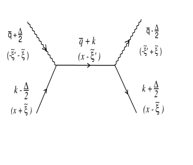
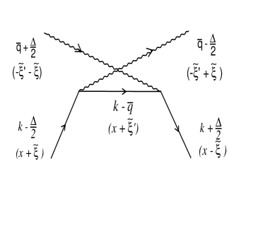
Figure 2: Leading order diagrams for the process $\gamma q\to\gamma q$. We indicate between parenthesis the $+$ components of the four-vectors.

The two diagrams of Fig. 2 have to be calculated. The leading order amplitude reads:

$$T_{H}^{TCS}\propto\frac{1}{(k+\bar{q})^{2}+i\epsilon}\gamma^{\nu}\>(\not{k}+\not{\bar{q}})\>\gamma^{\mu}$$

$$+\frac{1}{(k-\bar{q})^{2}+i\epsilon}\gamma^{\mu}\>(\not{k}-\not{\bar{q}})\>\gamma^{\nu}$$

$$\propto\frac{1}{2}\left[\not{n}\>(\tilde{p}^{\mu}n^{\nu}+\tilde{p}^{\nu}n^{\mu}-g^{\mu\nu})\>.\>(\frac{1}{x-\tilde{\xi^{\prime}}+i\epsilon}+\frac{1}{x+\tilde{\xi^{\prime}}-i\epsilon})\right.$$

$$\left.-\not{n}\gamma_{5}\>i\epsilon^{\mu\nu\kappa\lambda}\>n_{\lambda}\>\tilde{p}_{\kappa}\>\>(\frac{1}{x-\tilde{\xi^{\prime}}+i\epsilon}-\frac{1}{x+\tilde{\xi^{\prime}}-i\epsilon})\right].$$ (16)

The full TCS amplitude, corresponding to the diagram of Fig. 1-bottom (plus the associated crossed diagram) reads then

$$T^{TCS}=-\frac{e^{3}}{q^{\prime 2}}\>\bar{u}(k)\>\gamma^{\nu}\>v(k^{\prime})\>\epsilon^{\mu}(q)\>H_{\mu\nu}^{TCS},$$ (17)

with, in the Bjorken limit where $\xi=-\tilde{\xi}^{\prime}$,

$$H_{\mu\nu}^{TCS}$$ (18)

$$=\frac{1}{2}\>(-g_{\mu\nu})_{\perp}\int\limits_{-1}^{1}dx\>\left(\frac{1}{x-\xi-i\epsilon}+\frac{1}{x+\xi+i\epsilon}\right)$$

$$.\left(H(x,\xi,t)\bar{u}(p^{\prime})\not{n}u(p)+E(x,\xi,t)\bar{u}(p^{\prime})i\sigma^{\alpha\beta}n_{\alpha}\frac{\Delta_{\beta}}{2m}\>u(p)\right)$$

$$-\frac{i}{2}(\epsilon_{\nu\mu})_{\perp}\int\limits_{-1}^{1}dx\>\left(\frac{1}{x-\xi-i\epsilon}-\frac{1}{x+\xi+i\epsilon}\right)$$

$$.\left(\tilde{H}(x,\xi,t)\bar{u}(p^{\prime})\not{n}\gamma_{5}\>u(p)+\tilde{E}(x,\xi,t)\bar{u}(p^{\prime})\gamma_{5}\frac{\Delta.n}{2m}\>u(p)\right),$$

where we used the metric:

$$(-g_{\mu\nu})_{\perp}=-g_{\mu\nu}+\tilde{p}_{\mu}n_{\nu}+\tilde{p}_{\nu}n_{\mu}\>\>,$$ (19)

$$(\epsilon_{\nu\mu})_{\perp}=\epsilon_{\nu\mu\alpha\beta}\>n^{\alpha}\>\tilde{p}^{\beta}.$$

The GPDs entering Eq. 18 are proton GPDs, i.e. they read, in terms of quark flavors:

$$H_{TCS}(x,\xi,t)\,=\,{4\over 9}H^{u/p}\,+\,{1\over 9}H^{d/p}\,+\,{1\over 9}H^{s/p}.$$ (20)

In this work, we will take the GPD parametrizations from the VGG model Vanderhaeghen:1998uc ; Vanderhaeghen:1999xj ; goeke ; Guidal:2004nd , which are summarized in Ref. rpp and based on the Radyushkin double-distribution ansatz for the ($x$,$\xi$)-dependence Radyushkin:1998es ; Radyushkin:1998bz ; Mueller:1998fv and on a Reggeized ansatz for the $t$-distribution goeke ; Guidal:2004nd . At a couple of instances, in order to estimate the model dependence of our calculations, we will use the factorized ansatz for the $t$-dependence of the $H$ GPD Vanderhaeghen:1998uc . Also, we will occasionally study the sensitivity of observables to the so-called D-term Polyakov:1999gs , which is included in the VGG model and whose parametrization can be found as well in Refs. Vanderhaeghen:1998uc ; Vanderhaeghen:1999xj ; goeke ; Guidal:2004nd .

II.3 Gauge invariance

The TCS amplitude is not exactly gauge invariant, only in the Bjorken limit. To restore gauge invariance, twist-3 corrections of order $\Delta_{\perp}/Q$ are needed. As a first step in adressing this issue and estimating its effect, we propose to add a correction term to the twist-2 vector part tensor as follows:

$$H^{\mu\nu}=H^{\mu\nu}_{LO}-\frac{P^{\mu}}{2P\cdot\bar{q}}\cdot(\Delta_{\perp})_{\kappa}\cdot H^{\kappa\nu}_{LO}$$ (21)

$$+\frac{P^{\nu}}{2P\cdot\bar{q}}\cdot(\Delta_{\perp})_{\lambda}\cdot H^{\mu\lambda}_{LO}$$

$$-\frac{P^{\mu}P^{\nu}}{4(P\cdot\bar{q})^{2}}\cdot(\Delta_{\perp})_{\kappa}\cdot(\Delta_{\perp})_{\lambda}\cdot H^{\kappa\lambda}_{LO}\>,$$

where $H_{LO}^{\mu\nu}$ stands for the tensor of Eq. 18. This is a generalization of the prescription proposed in Refs. Vanderhaeghen:1999xj ; Guichon:1998xv for DVCS (we also refer the reader to Refs. Anikin:2000em ; Belitsky:2000vx ; Radyushkin:2000ap for further discussions on the issue of gauge invariance in the DVCS amplitude). One can readily check that $H^{\mu\nu}$ respects gauge invariance both w.r.t. initial and final photons, i.e. $q_{\mu}H^{\mu\nu}=0$, and $q^{\prime}_{\nu}H^{\mu\nu}=0$. The impact of adding this correction to the observables is shown at the end of this paper, in the section VII.

II.4 The Bethe-Heitler amplitude

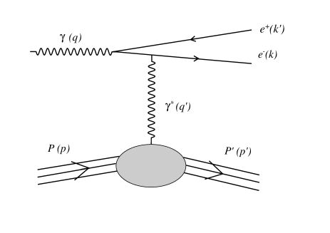
Figure 3: The Bethe-Heitler diagrams.

The TCS process is accompanied by the BH process, involving the two diagrams which are presented in Fig. 3. Their amplitude reads:

$$T^{BH}=-\frac{e^{3}}{\Delta^{2}}\>\bar{u}(p^{\prime})\>\Gamma^{\nu}\>u(p)\>\epsilon^{\mu}(q)\>\>$$ (22)

$$\bar{u}(k)\left(\gamma_{\mu}\frac{\not{k}-\not{q}}{(k-q)^{2}}\gamma_{\nu}+\gamma_{\nu}\frac{\not{q}-\not{k^{\prime}}}{(q-k^{\prime})^{2}}\gamma_{\mu}\right)\>v(k^{\prime}),$$ (23)

with the virtual photon-proton electromagnetic vertex matrix

$$\Gamma^{\nu}=\gamma^{\nu}\>F_{1}(t)+\frac{i\sigma^{\nu\rho}\Delta_{\rho}}{2\>m}\>F_{2}(t).\>$$ (24)

The BH amplitude depends on the proton Dirac and Pauli form factors $F_{1}(t)$ and $F_{2}(t)$ which, at small $t$ can be considered to be known with good accuracy. In this work, we take the parametrizations issued from Refs. Gayou:2001qd ; Brash:2001qq .

II.5 Cross section

At fixed beam energy $E_{\gamma}$ or longitudinal momentum transfer $\xi$, there are four independent kinematical variables for the process $\gamma(q)P(p)\to P^{\prime}(p^{\prime})e^{-}(k)e^{+}(k^{\prime})$. A natural choice is to take: $Q^{\prime 2}$ and $t=\Delta^{2}$ that we already defined, and the two angles $\theta$ and $\phi$ of the electron in the $\gamma^{*}$ center-of-mass (with the $z^{\prime}$-axis along the direction of the $\gamma^{*}$ in the $\gamma^{*}-P^{\prime}$ center of mass). We illustrate in Fig. 4 the different variables involved. In addition, we display the polarization angle $\Psi$ between the polarization vector of the incoming photon and the scattering plane in the $\gamma^{*}-p$ C.M..

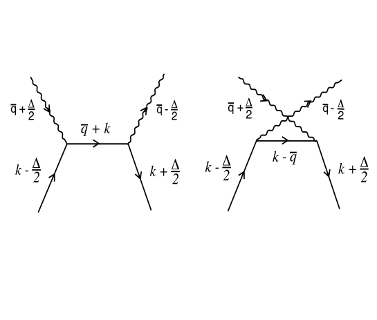
Figure 4: Top panel: scheme of the reaction plane $\gamma P\to\gamma^{*}P^{\prime}$ (for TCS) in the $\gamma P$ CM frame and illustration of some of the kinematic variables. Red arrows show the polarization vectors of the photon beam and proton target.
Bottom panel: decay angles in the $e^{-}e^{+}$ CM frame. $\phi$ and $\theta$ are respectively the azimuthal and polar angles between the $e^{-}$ direction and the virtual photon direction in the $\gamma^{*}-P^{\prime}$ CM frame.

The 4-differential unpolarized cross section is then expressed as:

$$\frac{d^{4}\sigma}{dQ^{\prime 2}dtd\Omega}({\gamma P\to P^{\prime}e^{+}e^{-}})$$ (25)

$$=\frac{1}{(2\pi)^{4}}\frac{1}{64}\frac{1}{(2mE_{\gamma})^{2}}\mid T^{BH}+T^{TCS}\mid^{2},$$

where $\mid T^{BH}+T^{TCS}\mid^{2}$ is averaged over the target proton helicities and beam polarizations and summed over the final proton helicities.

III Experimental considerations

The only data for the process $\gamma P\to P^{\prime}e^{-}e^{+}$ which are in the phase space of concern for our study, have been collected and analyzed a few years ago by the CLAS collaboration using the $\approx$ 6 GeV electron beam of Jefferson Lab. The data were actually obtained in “quasi-photoproduction” mode. This means that the scattered electron from the beam is not detected in CLAS and is considered to be in almost the same direction as the beamline. This results in very low $Q^{2}$ electroproduction, i.e. “quasi-photoproduction”. This pilot analysis can be found in Ref. Rafo . The $\approx$ 6 GeV beam energy, combined with the $\approx$ 10³⁴cm^-2s^-1 luminosity, allowed to reach maximum $Q^{\prime 2}$ values of 3 GeV², which corresponds to an invariant mass of the $e^{+}e^{-}$ system $M_{e^{+}e^{-}}$ of $\approx$ 1.8 GeV. This is close to the mass of several vector mesons decaying into $e^{+}e^{-}$, in particular the broad $\rho^{\prime}$(1700). In order to have a TCS interpretation as clean as possible, it is of course advisable to avoid such resonances which contribute to the process $\gamma P\to P^{\prime}e^{-}e^{+}$. The data analysis of Ref. Rafo is therefore difficult to interpret in terms of GPDs but it nevertheless demonstrates that the process $\gamma P\to P^{\prime}e^{-}e^{+}$ can be measured at JLab.

The forthcoming JLab energy upgrade to 11 GeV allows to explore a $Q^{\prime 2}$ region between 4 and 9 GeV² which corresponds to a $M_{e^{+}e^{-}}$ region between 2 and 3 GeV, i.e. a vector meson resonance-free region between the $\rho^{\prime}$ and the $J/\Psi$. In the case of CLAS12, the upgraded CLAS detector associated to the JLab energy increase, there is also a luminosity gain of a factor 10. These upgrades have led to the first dedicated TCS accepted proposal at JLAB  JLABprop . It will use a similar “quasi-photoproduction” technique as used in the pioneer 6 GeV analysis. In addition, there will be the improvement of the detection of the low $Q^{2}$ scattered electron via a dedicated tagging equipement, supplementing CLAS12. This allows, besides the measurement of unpolarized cross sections, to obtain linearly polarized photons observables, by measuring the azimuthal dependence of the scattered electron. Finally, with a polarized electron beam, which is available at JLab, one can access circularly polarized photons observables. It is therefore expected that in the next few years, numerous $\gamma P\to P^{\prime}e^{-}e^{+}$ data which can lend to GPD interpretation will be available.

We show in Fig. 5 the kinematical domain which can be accessed with the upgraded JLab. We display in blue the ($\xi$, $Q^{\prime 2}$) phase space accessible for TCS with an 11 GeV electron beam, assuming that the real photon is provided by bremsstrahlung of the electron and that its energy is in $E_{\gamma}\in[5,11]$ GeV. We have applied two cuts: $Q^{\prime 2}\in[4,9]$ GeV² and $-t\in[0,1]$ GeV². The motivations are respectively to stay in the region free of vector mesons resonances and minimize higher twist corrections to the TCS formalism, which grow with $\frac{t}{Q^{\prime 2}}$. We overlap in red in this same figure the ($\xi$, $Q^{2}$) phase space accessible with an 11 GeV beam for DVCS. We have applied the cuts: $-t\in[0,1]$ GeV², for the same reason as for TCS, and $s>4$ GeV² in order to stay above the baryon resonance region.

One notes the large intersection between the DVCS and the TCS phase spaces. Measurements of observables sensitive to GPDs in the common ($\xi,Q^{2}$) region by both processes should bring strong constraints on the extraction of GPDs and tests of factorization and universality.

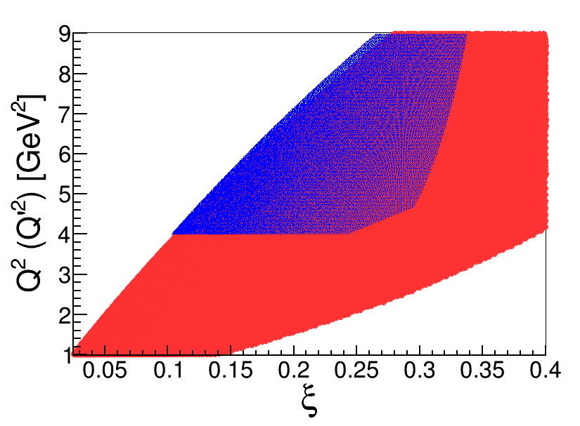
Figure 5: Kinematical domain accessible as a function of $\xi$ and $Q^{2}$ for DVCS (red plain surface) and in $\xi$ and $Q^{\prime 2}$ for TCS (blue dotted surface) with an 11 GeV electron beam. For DVCS, the cuts $-t\in[0,1]$ GeV² and $s>4$ GeV² have been applied and for TCS, the cuts $E_{\gamma}\in[5,11]$ GeV, $-t\in[0,1]$ GeV² and $Q^{\prime 2}\in[4,9]$ GeV² have been applied.

We now present our results for the calculations of the unpolarized cross sections, single spin asymmetries and double-spin asymmetries, respectively in sections  IV,  V and  VI. In these sections, all calculations will be done in the Bjorken limit and at leading order (we refer the reader to Refs. Pire:2011st ; Muller:2012yq ; Moutarde:2013qs for works on Next-To-Leading order corrections in $\alpha_{s}$ to the TCS amplitude). In section  VII, we will study the effect of keeping the exact kinematics presented in section II.1 and of the gauge-invariance restoration prescription described in section II.3.

IV Unpolarized cross section

We discuss in this section the unpolarized cross section of the $\gamma P\to P^{\prime}e^{+}e^{-}$ process, which therefore includes the BH and TCS processes. Fig. 6 shows our calculation of the $\phi$-dependence of the 4-fold differential cross section $\frac{d\sigma_{BH}}{dQ^{\prime 2}\>dt\>d\phi\>d(cos\theta)}$ at $\xi=0.2$, $-t=0.4$ GeV², $Q^{\prime 2}=7$ GeV² and for different $\theta$ values. The $\phi$-shape is strongly dependent on the $\theta$ value. As $\theta$ tends to $0^{\circ}$, the $\phi$ distribution peaks towards $\phi$=180^∘ and as $\theta$ tends to 180^∘, the $\phi$-distribution peaks towards $\phi$=0^∘ (or 360^∘). There is a smooth transition between these two singularities for the intermediate $\theta$ values. For instance, at $\theta$=90^∘, the calculation shows only two small “bumps” at $\phi$=0^∘ and $\phi$=180^∘.

These particular shapes are due to the BH process and its singularities. Indeed, in the BH diagrams of Fig. 3, when the electron (positron) is emitted in the direction of the initial photon, i.e. $\theta$=0^∘ ($\theta$=180^∘), the propagator of the positron (electron) becomes singular and creates a peak in the $\phi$ distribution at $\phi$=180^∘ ($\phi$=0^∘). Intuitively, $\theta$=0^∘ ($\theta$=180^∘) forces all particles to be in the same plane, i.e. $\phi$=180^∘ ($\phi$=0^∘). The kinematics $\theta$=0^∘, i.e. the electron is in the direction of the photon beam, corresponds to $\phi$=180^∘ because the virtual photon is emitted by the positron, not the electron (see Fig. 6).

We display also in Fig. 6 the contribution of TCS alone. In this calculation, we have used only the GPD $H$. The inclusion of the other GPDs barely changes the curves. In contrast to the BH, the TCS is almost flat in $\phi$ for all $\theta$ values. It is clear that the process $\gamma P\to P^{\prime}e^{+}e^{-}$ is largely dominated by the BH. There is never less than an order of magnitude between BH and TCS.

In Fig. 6, we show the curves BH+TCS for a series of $\theta$ angles as well as the BH alone for $\theta$=45^∘ and $\theta$=90^∘. Only at $\theta$=90^∘, where one is far from the two BH singularities, we have a visible difference between the two curves and therefore a sensitivity to TCS. It is of the order of 30% at $\phi$=180^∘. As one gets closer to one of the two BH singularities ($\theta$=45^∘ for instance), the two curves BH and BH+TCS are essentially indistinguishable and there is no sensitivity to TCS.

Finally, we show in Fig. 6, our calculations of BH+TCS (and of BH alone) for $\theta$ integrated over the range $[\pi/4,3\pi/4]$. In order to maximize count rates, from an experimental point of view, it is interesting to integrate over $\theta$. We still have a sensitivity to TCS, however it is of the order of 5%, i.e. lesser than at fixed $\theta$=90^∘: the integration over $\theta$ dilutes the sensitivity to TCS.

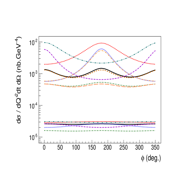
Figure 6: Unpolarized cross section $\frac{d\sigma}{dQ^{\prime 2}\>dt\>d\phi\>d(cos\theta)}$ for the process $\gamma P\to P^{\prime}e^{+}e^{-}$ (for BH + TCS and TCS alone) as a function of $\phi$, at $\xi$=0.2, $-t=0.4$ GeV², $Q^{\prime 2}=7$ GeV² for different fixed $\theta$ values: $10^{\circ},45^{\circ},\>90^{\circ},\>135^{\circ},\>170^{\circ}$ and for $\theta$ integrated over $[\pi/4,3\pi/4]$. For two values of $\theta$ ($45^{\circ}$ and $90^{\circ}$) and for $\theta$ integrated over $[\pi/4,3\pi/4]$, we also show the calculation of the BH alone.

We display in the top panel of Fig. 7 the $Q^{\prime 2}$-dependence, at $\xi=0.2$ and $-t=0.4$ GeV², of $d\sigma/dQ^{\prime 2}dt$ for the BH and TCS processes. The 2-fold cross section has been integrated over the decay angles: $\phi\in[0,2\pi]$ and $\theta\in[\frac{\pi}{4},\frac{3\pi}{4}]$. We also display in this figure the results of the analytical formulaes of Ref. Berger:2001xd . For TCS, we have of course used the same GPD parameterization for both calculations (only $H$ in this case).

In order to better appreciate the comparison, we display in the bottom panel of Fig. 7 the ratios of our calculations to those of Ref. Berger:2001xd . The agreement is excellent for the BH process, as it should, since there was no approximation done in the derivation of the analytical formula for this process in Ref. Berger:2001xd . For TCS, we show two curves for the ratio. Indeed, in Ref. Berger:2001xd , in the analytical formula for the TCS process, the nucleon mass was neglected in the phase space factor, i.e. the cross section is proportional to ${1}\over{s^{2}}$ rather than ${1}\over{s-m^{2}}^{2}$ (this is not the case for the BH process where the phase space factor is exact in Ref. Berger:2001xd ). In the bottom panel of Fig. 7, we plot the TCS cross section of Ref. Berger:2001xd with (blue dotted curve) and without (red dashed curve) the nucleon mass term in the phase space factor. In this way, one can distinguish the differences between the two calculations originating from the trivial phase space factor from those, more subtle, coming from the TCS amplitude. It is seen in this figure that at the lowest $Q^{\prime 2}$ values and at the presently considered kinematics, the difference in the cross section calculations depending on the prescription taken for the phase space factor can reach more than 10%. In both cases, it is also seen that the difference between the Berger et al.’s calculations and ours diminishes as $Q^{\prime 2}$ increases, as expected since terms of the order of ${m^{2}}\over{Q^{\prime 2}}$ were dropped in the TCS analytical formula of Ref. Berger:2001xd .

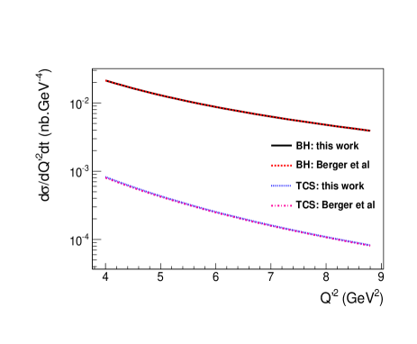
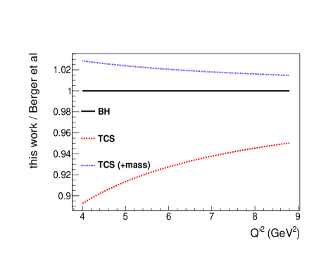
Figure 7: Top panel: the two-fold differential cross section $d\sigma/dQ^{\prime 2}dt$ for BH (highest curves) and TCS (lowest curves) as a function of $Q^{\prime 2}$ for $\xi=0.2$ and $-t=0.4$ GeV². The calculations have been integrated over $\phi\in[0,2\pi]$ and $\theta\in[\frac{\pi}{4},\frac{3\pi}{4}]$. The solid curves are our calculations while the dashed curves are from Ref. Berger:2001xd . Bottom panel: ratio of our calculations to those of Ref. Berger:2001xd . For the TCS process, the blue dotted curve contains the nucleon mass term in the phase space factor in the calculation of Ref. Berger:2001xd while the red dashed curve does not.

To end this section concerning the unpolarized cross section, we show in Fig. 8 the influence of the D-term on the three-fold differential cross section $d\sigma/dQ^{\prime 2}dtd\phi$, calculated for $\xi=0.2$, $-t=0.4$ GeV² and with $\theta$ integrated over $[\frac{\pi}{4},\frac{3\pi}{4}]$. It modifies the amplitude of the cross section at $\phi=0^{\circ}$ and $\phi=180^{\circ}$ by about 10%.

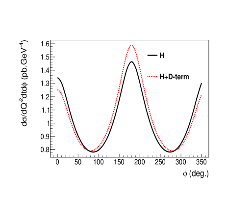
Figure 8: The three-fold differential cross section $d\sigma/dQ^{\prime 2}dtd\phi$ as a function of $\phi$ with (red dashed curve) and without (black solid curve) the D-term, calculated at $\xi=0.2$, $-t=0.4$ GeV² and with $\theta$ integrated over $[\frac{\pi}{4},\frac{3\pi}{4}]$.

V Single spin asymmetries

We now turn to the single spin asymmetries: beam or target. Photons beams can be polarized linearly or circularly. Target polarization vectors can be oriented along the $x-$, $y-$ or $z-$axis in the $\gamma P\to\gamma^{*}P^{\prime}$ plane (see Fig. 4). For polarization observables, we will calculate spin asymmetries and, following notations used for DVCS, we will tag them $A_{ij}$, i.e. with two indices $i$ and $j$. The first index $i$ refers to the polarization type of the beam: $U$ for an unpolarized beam, $\odot$ for a circularly polarized beam and $\ell$ for a linearly polarized beam. The second index $j$ refers to the polarization of the target and can take the values $U$, $x$, $y$ or $z$, with obvious meanings. In this section, dedicated to single-polarization observables, we will therefore consider successively the five independent asymmetries $A_{\ell U}$, $A_{\odot U}$, $A_{Ux}$, $A_{Uy}$ and $A_{Uz}$.

V.1 Linearly polarized photons

We introduce the angle $\Psi$ between the polarization vector of the photon and the plane spanned by the photon beam and the ($e^{+}e^{-}$) system, which contains the $x$-axis (see Fig. 4). Then, we define:

$$A_{\ell U}(\Psi)=\frac{\sigma_{x}(\Psi)-\sigma_{y}(\Psi)}{\sigma_{x}(\Psi)+\sigma_{y}(\Psi)},$$ (26)

where $\sigma_{x}$ ($\sigma_{y}$) stands for the 4-fold differential cross sections $\frac{d\sigma}{dQ^{\prime 2}\>dt\>d\phi\>d(cos\theta)d\Psi}$ with a photon beam polarized in the $x$-($y$-)direction. We display in Fig. 9 the $\Psi$-dependence of $A_{\ell U}$ for $\xi$=0.2, $-t=0.2$ GeV², $Q^{\prime 2}=7$ GeV² for $\theta=45^{\circ}$, $\theta=90^{\circ}$ and $\theta$ integrated over $[\pi/4,3\pi/4]$ and $\phi=0^{\circ}$ and $\phi=10^{\circ}$. The approximate shape of the asymmetry is a $\cos(2\Psi)$ which is reminiscent of the modulation which is predicted for the so-called $\Sigma$ asymmetry in single meson photoproduction. This $\cos(2\Psi)$ modulation appears explicitely in the analytical expressions of Ref. Goritschnig .

We note that the BH alone produces an asymmetry. It is actually the dominant contribution. The TCS produces only variations of the amplitude at the percent level around the BH, making this observable not very favorable to study TCS and GPDs. The amplitude and phase of the asymmetry depend strongly on the decay angles: it is the strongest as $\theta$ approaches 90^∘ and the phase increases as $\phi$ increases. This phase shift due to $\phi$ is also apparent in Ref. Goritschnig .

In Fig. 9, we have used only the contribution of the $H$ GPD for TCS. In Fig. 10, we show the $t$-dependence of the $A_{\ell U}$ asymmetry for BH alone, BH+TCS (with only $H$) and BH+TCS (with $H$+$\tilde{H}$). Calculations have been done for $\xi$=0.2, $Q^{\prime 2}=7$ GeV², $\phi=0^{\circ}$, $\Psi=180^{\circ}$ and for $\theta=45^{\circ}$, $\theta=90^{\circ}$ and $\theta$ integrated over $[\pi/4,3\pi/4]$. Depending on $t$, we notice some sensitivity of the $A_{\ell U}$ observable to the GPDs $H$ and $\tilde{H}$.

In Fig. 11, we show the peculiar $\phi$-dependence of $A_{\ell U}$ at $\Psi=0^{\circ}$ at our standard kinematics. We also show the (small) influence of the D-term.

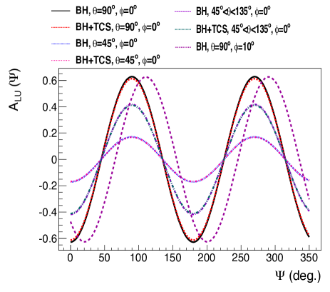
Figure 9: $A_{\ell U}$ asymmetry as a function of $\Psi$ for BH and for BH+TCS (only GPD $H$ contribution) at $\xi$=0.2, $-t=0.4$ GeV², $Q^{\prime 2}=7$ GeV² and for different sets of $\theta$ and $\phi$ angles.

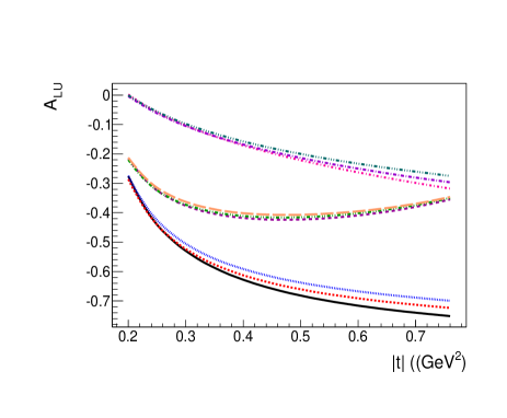
Figure 10: $A_{\ell U}$ asymmetry as a function of $t$ for $\xi$=0.2, $Q^{\prime 2}=7$ GeV², $\Psi=0^{\circ}$, $\phi=0^{\circ}$ and $\theta=45^{\circ}$, $\theta=90^{\circ}$ and $\theta\in[\pi/4,3\pi/4]$.

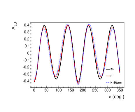
Figure 11: $A_{\ell U}$ asymmetry as a function of $\phi$ for $\xi=0.2$, $Q^{\prime 2}=7$ GeV², $-t=0.4$ GeV² and $\theta\in[\pi/4,3\pi/4]$. The black solid curve corresponds to BH only, the red dashed curve to BH+TCS with only the GPD $H$ contribution and the blue dotted curve to BH+TCS with the GPD $H$ and the D-term contributions.

V.2 Circularly polarized photons

We define:

$$A_{\odot U}=\frac{\sigma^{+}-\sigma^{-}}{\sigma^{+}+\sigma^{-}},$$ (27)

where $\sigma^{\pm}$ stand for the 4-fold differential cross sections $\frac{d\sigma}{dQ^{\prime 2}\>dt\>d\phi\>d(cos\theta)}$ for the two photon spin states, right and left polarized.

We display in Fig. 12 (top panel) our results for $A_{\odot U}$ as a function of $\phi$ at $Q^{\prime 2}=7$ GeV², $\xi=0.2$, $-t=0.4$ GeV² for $\theta$=45^∘, 90^∘ and $\theta$ integrated over $[45^{\circ},135^{\circ}]$. The TCS is calculated here with only the $H$ GPD. In all kinematics, we obtain a $\sin(\phi)$ shape with a significant amplitude, up to $\approx$ 25%. We observe that the BH doesn’t produce any asymmetry. Any signal therefore reflects a contribution from TCS. This is due to the fact that, as was shown in Ref. Berger:2001xd , this observable is sensitive to the imaginary part of the amplitude and that the BH amplitude is purely real. The amplitude of the asymmetry depends on $\theta$. It is maximal for $\theta$=90^∘ where BH is minimal and it decreases as $\theta$ tends to $\theta$=0^∘ (or 180^∘). Since the BH does not produce on its own an asymmetry, one sees that the integration over $\theta$ does not strongly reduce the signal. Such integration allows to maximize count rates.

In Fig. 12 (top panel), we also compare our results to those of Ref. Berger:2001xd . In all cases, our calculations produce amplitudes a few percents larger. This might be attributed to some mass correction terms to the TCS amplitude which are present in our calculation and not in Ref. Berger:2001xd .

Fig. 12 (bottom panel) shows the $A_{\odot U}$ asymmetry for $\theta$ integrated over $[45^{\circ},135^{\circ}]$ using different GPDs parametrizations for TCS.

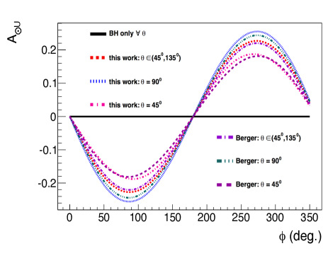
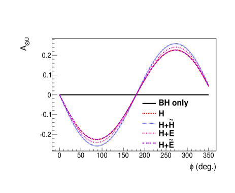
Figure 12: Top panel: The $A_{\odot U}$ asymmetry as a function of $\phi$ for $\theta=45^{\circ}$, $\theta=90^{\circ}$ and $\theta\in[45^{\circ},135^{\circ}]$. The TCS is calculated here with only the $H$ GPD. We compare our calculations to those of Ref. Berger:2001xd . Bottom panel: The $A_{\odot U}$ for $\theta\in[45^{\circ},135^{\circ}]$ using differents GPDs parametrizations for TCS. The calculations are done for $Q^{\prime 2}=7$ GeV², $\xi=0.2$, $-t=0.4$ GeV².

In Fig. 13, we show for $\xi=0.2$, $Q^{\prime 2}=7$ GeV², $\phi=90^{\circ}$ and $\theta$ integrated over $[45^{\circ},135^{\circ}]$, the $t$-dependence of $A_{\odot U}$ and its sensitivity to different GPDs. We notice that the magnitude of $A_{\odot U}$ increases with $|t|$ and that there is a sensitivity of this observable to all four GPDs, especially at large $\mid t\mid$. We also display in this figure our calculation with the factorized ansatz for the $t$-dependence of the $H$ GPD in order to illustrate the model-dependence of our results.

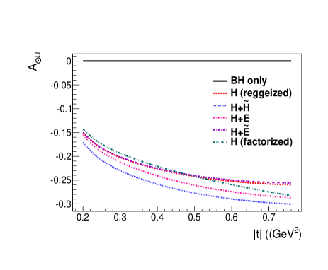
Figure 13: The $A_{\odot U}$ asymmetry as a function of $t$ for BH+TCS at $\xi=0.2$, $Q^{\prime 2}=7$ GeV², $\phi=90^{\circ}$ and $\theta$ integrated over $[45^{\circ},135^{\circ}]$. TCS is calculated with different GPD contributions.

V.3 Polarized targets

We define:

$$A_{Ui}=\frac{\sigma^{+}-\sigma^{-}}{\sigma^{+}+\sigma^{-}},$$ (28)

where $\sigma^{\pm}$ stands for the four-fold differential cross sections $\frac{d\sigma}{dQ^{\prime 2}\>dt\>d\phi\>d(cos\theta)}$ for the two target spin orientations $+$ and $-$ along the axis $i=x,y$ or $z$.

We show in Fig. 15 our results for the $\phi$-dependence of $A_{Ux}$, $A_{Uy}$ and $A_{Uz}$ for $Q^{\prime 2}=7$ GeV², $\xi=0.2$, $-t=0.4$ GeV² for $\theta$ integrated over $[\frac{\pi}{4},\>\frac{3\pi}{4}]$. Like for $A_{\odot U}$, it is advantageous to integrate over $\theta$, in order to maximize count rates, since the signal is barely reduced. The TCS is calculated with different GPD contributions. We observe $\sin\phi$ or $\cos\phi$ shapes with amplitudes between 10 and 15%. Like for $A_{\odot U}$, the BH doesn’t produce any asymmetry and any non-zero asymmetry directly reflects the strength of GPDs.

We show in Fig. 15 the $t$-dependence of $A_{Ux}$, $A_{Uy}$ and $A_{Uz}$ at $\phi$=90^∘, 0^∘ and 90^∘ respectively, for the kinematics $\xi=0.2$, $Q^{\prime 2}=7$ GeV² and $\theta$ integrated over $[\frac{\pi}{4},\>\frac{3\pi}{4}]$. In this figure, TCS is calculated with different GPDs. Depending on the value of $t$, the three asymmetries are sensitive to the GPDs $H$, $\tilde{H}$ and $E$ in various proportions. We also display in this figure our calculation with the factorized ansatz for the $t$-dependence of the $H$ GPD in order to illustrate the model-dependence of our results.

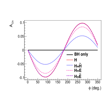
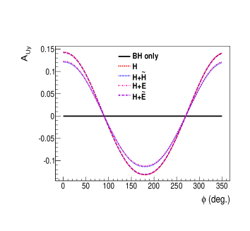
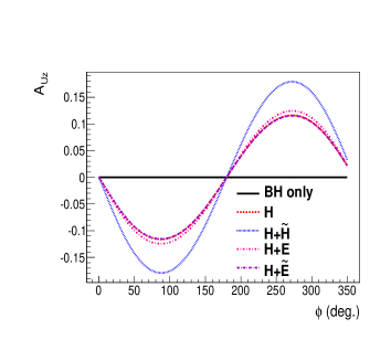
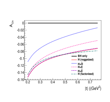
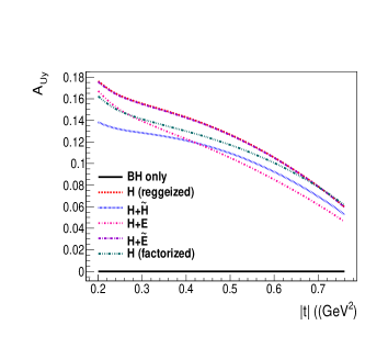
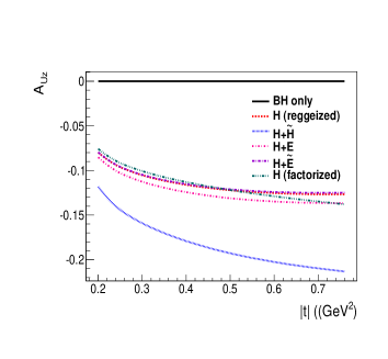
Figure 14: The $A_{Ux}$ (left panel), $A_{Uy}$ (central panel) and $A_{Uz}$ (right panel) asymmetries as a function of $\phi$ for $\xi=0.2$, $Q^{\prime 2}=7$ GeV², $-t=0.4$ GeV² and for $\theta$ integrated over $[\frac{\pi}{4},\>\frac{3\pi}{4}]$. The TCS is calculated with different GPDs contributions.

Figure 15: The $A_{Ux}$ (left panel), $A_{Uy}$ (central panel) and $A_{Uz}$ (right panel) asymmetries as a function of $t$, at $\phi$=90^∘, 0^∘ and 90^∘ respectively, and for $\xi=0.2$, $Q^{\prime 2}=7$ GeV², $-t=0.4$ GeV² and $\theta$ integrated over $[\frac{\pi}{4},\>\frac{3\pi}{4}]$. TCS is calculated with different GPD contributions.

VI Double spin asymmetries

We define the double-spin asymmetries:

$$A_{ij}=\frac{(\sigma^{++}+\sigma^{--})-(\sigma^{+-}+\sigma^{-+})}{\sigma^{++}+\sigma^{--}+\sigma^{+-}+\sigma^{-+}},$$ (29)

where $\sigma^{\pm\pm}$ stand for the four-fold differential cross sections $\frac{d\sigma}{dQ^{\prime 2}\>dt\>d\phi\>d(cos\theta)}$ for the two photon beam spin states $+$ and $-$ (first index) and the two target spin orientations $+$ and $-$ (second index) along the target polarization axis. The first index of $A$ refers to the polarization nature of the photon beam ($i=\ell$ for a linear polarization and $i=\odot$ for a circular polarization) and the second index refers to the axis polarization of the target $j=x,y$ or $z$. We present and discuss in the two following subsections our results for $A_{\odot j}$ and $A_{\ell j}$.

VI.1 Circularly polarized photons and polarized target

Fig. 17 shows our results for $A_{\odot x}$, $A_{\odot y}$ and $A_{\odot z}$, from left to right, as a function of $\phi$ at the kinematics $\xi=0.2$, $-t=0.4$ GeV², $Q^{\prime 2}=7$ GeV². The top row shows the result of our calculations for $\theta$ integrated over $[\frac{\pi}{4},\>\frac{3\pi}{4}]$ with different GPD contributions to the TCS amplitude. The bottom row shows the same observables with only the GPD $H$ contribution for different $\theta$ angle sets.

One notes that the BH process alone produces asymmetries in all cases. The $\phi$-shapes of the asymmetries are complex and very dependent on $\theta$. Also, in contrast to the single spin asymmetries that we studied in the previous section, the $\phi$-shapes are also very dependent on the specific GPDs entering the TCS process. One notes in particular important sensitivities to the $H$, $\tilde{H}$, $\tilde{E}$ GPDs as well as to the D-term. Furthermore, one also notes the sensitivity of these double-polarization observables to the ansatz used for the $t$-dependence.

Fig. 17 shows the $t$-dependence of the double spin asymmetries $A_{\odot x}$, $A_{\odot y}$ and $A_{\odot z}$ at $\phi=0^{\circ}$, $\phi=90^{\circ}$ and $\phi=0^{\circ}$ respectively, at the kinematics $\xi=0.2$, $Q^{\prime 2}=7$ GeV² and $\theta$ integrated over $[\pi/4,3\pi/4]$. We also display in this figure our calculation with the factorized ansatz for the $t$-dependence of the $H$ GPD in order to illustrate the model-dependence of our results. The change of sign for $A_{\odot y}$ for the factorized ansatz compared to the Reggeized ansatz is in particular remarkable. As can be seen in the top panel of Fig. 17, this is due to the fact that the factorized model crosses the “zero” line before $\phi=90^{\circ}$ while the Reggeized model crosses it after, thus producing respectively positive and negative $A_{\odot y}$’s at $\phi=90^{\circ}$.

VI.2 Linearly polarized photons and polarized target

Fig. 18 shows our results for the double-spin asymmetries $A_{\ell x}$, $A_{\ell y}$ and $A_{\ell z}$, from left to right, as a function of $\phi$ at the kinematics $\xi=0.2$, $-t=0.4$ GeV², $Q^{\prime 2}=7$ GeV² with $\theta$ integrated over $[\frac{\pi}{4},\>\frac{3\pi}{4}]$.

One notes that the BH process alone produces a null asymmetry in all cases, making this double-spin asymmetry particularly favorable to study TCS and GPDs. $A_{\ell y}$ is mostly sensitive to the GPD $H$ contribution while $A_{\ell x}$ and $A_{\ell z}$ show a sensitivity to the GPD $\tilde{H}$ as well.

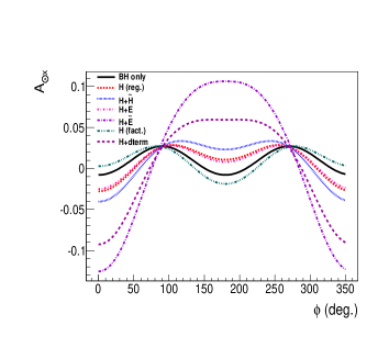
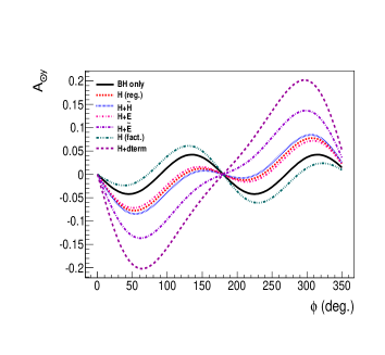
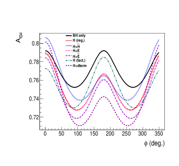
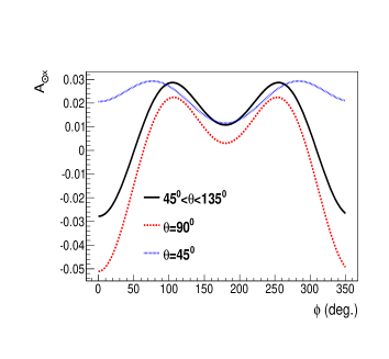
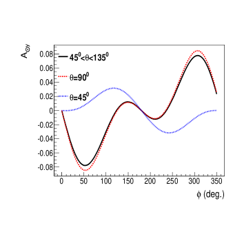
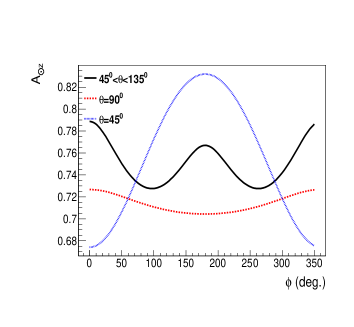
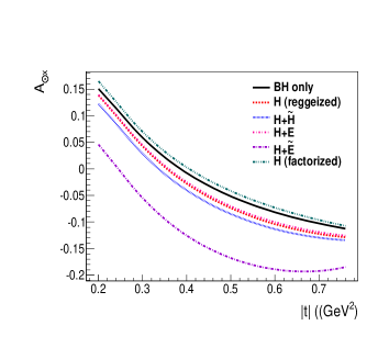
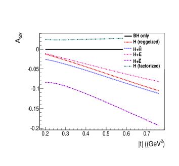
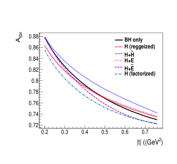
Figure 16: Circularly polarized beam-target double spin asymmetries as a function of $\phi$ at $\xi=0.2$, $-t=0.4$ GeV² and $Q^{\prime 2}=7$ GeV². Left column: $A_{\odot x}$, central column: $A_{\odot y}$, right column: $A_{\odot z}$. In the top row panels, $\theta$ integrated over $[\frac{\pi}{4},\>\frac{3\pi}{4}]$ and the calculations are done for different GPD contributions to the TCS process. In the bottom row panels, the calculations are done for different $\theta$ angles: $\theta=90^{\circ}$ (red dashed curve), $\theta=45^{\circ}$ (blue dotted curve) and $\theta$ integrated over $[\frac{\pi}{4},\>\frac{3\pi}{4}]$ (black solid curve) and with the GPD $H$ (Reggeized) contribution only.

Figure 17: Circularly polarized beam-target double spin asymmetries as a function of $t$. Left: $A_{\odot x}$, center: $A_{\odot y}$, right: $A_{\odot z}$. Calculations are done at the kinematics: $\xi=0.2$, and $Q^{\prime 2}=7$ GeV² and $\phi$=0^∘ ($A_{\odot x}$), $\phi=90^{\circ}$ ($A_{\odot y}$) and $\phi=0^{\circ}$ ($A_{\odot z}$). $\theta$ is integrated over $[\frac{\pi}{4},\>\frac{3\pi}{4}]$ in these calculations.

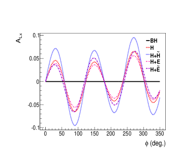
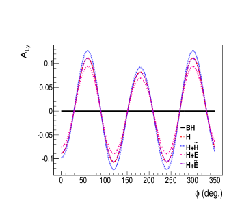
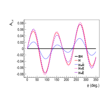
Figure 18: Linearly polarized beam-target double spin asymmetries as a function of $\phi$ at $\xi=0.2$, $-t=0.4$ GeV² and $Q^{\prime 2}=7$ GeV² and $\theta$ integrated over $[\frac{\pi}{4},\>\frac{3\pi}{4}]$ for different GPD contributions. Left column: $A_{\ell x}$, central column: $A_{\ell y}$, right column: $A_{\ell z}$.

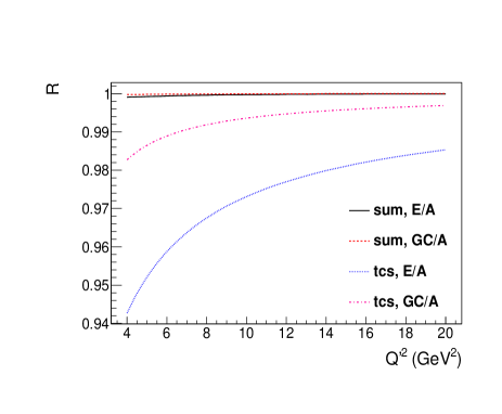
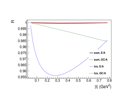
Figure 19: $Q^{\prime 2}$-dependence (left panel) and $|t|$-dependance (right panel) of the ratio of the 2-fold cross differential cross sections $d\sigma/dtdQ^{\prime 2}$ of Bethe-Heitler and of TCS (integrated over the decay angles: $\phi\in[0,2\pi]$ and $\theta\in[\frac{\pi}{4},\frac{3\pi}{4}]$) calculated with the gauge invariance restoration term (dot-dashed curve for TCS: gauge invariant/asymptotic) and with the exact kinematics (dotted curve for TCS: ”exact”/asympototic) to the asymptotic limit (i.e. Bjorken limit) calculation. The calculation has been carried out for $\xi=0.1$, $\theta$ is integrated over $[\pi/4,3\pi/4]$, $\phi$ is integrated over $[0,2\pi]$ and at $-t=0.4$ GeV² (left panel) or at $Q^{\prime 2}=7$ GeV² (right panel).

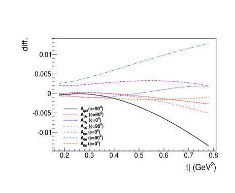
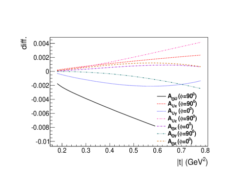
Figure 20: Difference of the single and double spin asymmetries (circularly polarized photon) as a function of $|t|$ before and after the corrections. Left panel: with the exact kinematic compared to the asymptotic limit. Right panel: with the gauge invariance restoration term compared to the asymptotic limit. The calculations have been carried out for $\xi=0.2$, $-t=0.4$ GeV², $Q^{\prime 2}=7$ GeV² and $\theta$ has been integrated over $[\pi/4,3\pi/4]$. The different $\phi$ angles are indicated on the figure.

VII Corrections to the leading-twist calculations

We evaluate in this final section two types of higher-twist corrections: keeping the exact kinematics presented in section II.1, i.e. $\mid\tilde{\xi\mid}\neq\mid\xi\mid\neq\mid\tilde{\xi}^{\prime}\mid\neq\mid\xi^{\prime}\mid$, and adding the gauge correction term of section II.3 to the TCS tensor.

Fig. 19 shows the $Q^{\prime 2}$-dependence and the $|t|$-dependence of the ratio of the 2-fold cross differential cross sections $d\sigma/dtdQ^{\prime 2}$ for Bethe-Heitler and for TCS (integrated over the decay angles: $\phi\in[0,2\pi]$ and $\theta\in[\frac{\pi}{4},\frac{3\pi}{4}]$) calculated with the gauge invariance restoration term (dot-dashed curve for TCS) and with the exact kinematics (dotted curve for TCS) to the asymptotic limit (i.e. Bjorken limit) calculation that we have presented so far. The calculation has been carried out for $\xi=0.1$ and at $-t=0.4$ GeV² (left panel) or at $Q^{\prime 2}=7$ GeV² (right panel). One sees that these ratios tend to 1 as $Q^{\prime 2}$ increases and as $|t|$ decreases, as expected. The effects of these corrections in the domains of current interest, covered in this figure, are of the order of a few percents for TCS. The exact kinematic corrections are more important (always less than 6% though) than the gauge invariance restoring corrections.

We show in Fig. 19 that the impact of these corrections on the asymmetries that we discussed earlier is of the order of 0.1% to 1% and don’t affect the conclusions that we drew earlier.

VIII Conclusion

In this work, we have studied the $\gamma P\to P^{\prime}e^{+}e^{-}$ process in terms of GPDs in a regime where one can expect to access them. We have presented our derivations of the TCS and BH amplitudes both contributing to the $\gamma P\to P^{\prime}e^{+}e^{-}$ process and calculated all unpolarized, single beam, single target and double beam-target spin observables.

We show that, since the TCS process is lower by several factors in the unpolarized cross section compared to the BH process, it is judicious to measure spin asymmetries which reveal a more direct sensitivity to GPDs. In particular, the BH process alone doesn’t produce any signal for the target single spin asymmetries, for the circularly polarized beam single spin asymmetries and for the linearly polarized photons and polarized target double spin asymmetries. These observables are therefore particularly favorable to directly measure GPD strength. We have shown in general that the various single- and double-polarization observables that we have calculated show different sensitivities to the four GPDs, which should ultimately allow to disentangle them with some adequate GPD fitting algorithms. We also provided first estimations of higher-twist contributions such as keeping the exact kinematics and including a gauge invariance restoring term. The effects are at the level of a few percent on cross sections and spin asymmetries.

A rich new experimental TCS program can be envisioned with the forthcoming JLab energy upgrade, which would complement the DVCS program already approved in order to access GPDs. All of the TCS observables that we calculated in this work should be measurable and can serve as a basis for developping experimental proposals. This work might also find some applications at higher energies, like at hadron colliders, such as LHC and RHIC, in ultraperipheral collisions Pire:2008ea or at the projected electron-ion collider EIC Accardi:2012qut .

References

- (1) K. Goeke, M. V. Polyakov and M. Vanderhaeghen, Prog. Part. Nucl. Phys. 47 401 (2001).
- (2) M. Diehl, Phys. Rept. 388 41 (2003).
- (3) A.V. Belitsky, A.V. Radyushkin, Phys. Rept. 418 1 (2005).
- (4) M. Guidal, H. Moutarde and M. Vanderhaeghen, Rept. Prog. Phys. 76 066202 (2013).
- (5) E. R. Berger, M. Diehl and B. Pire, Eur. Phys. J. C 23 675 (2002).
- (6) A. T. Goritschnig, B. Pire and J. Wagner, arXiv:1404.0713 [hep-ph].
- (7) X. Ji, Phys.Rev.Lett. 78, 610 (1997); Phys.Rev.D 55, 7114 (1997).
- (8) M. Vanderhaeghen, P.A.M. Guichon and M. Guidal, Phys. Rev. Lett. 80 5064 (1998)
- (9) M. Vanderhaeghen, P. A. M. Guichon and M. Guidal, Phys. Rev. D 60 094017 (1999).
- (10) M. Guidal, M. V. Polyakov, A. V. Radyushkin and M. Vanderhaeghen, Phys. Rev. D 72 054013 (2005).
- (11) A. V. Radyushkin, Phys. Rev. D 59 014030 (1999).
- (12) A. V. Radyushkin, Phys. Lett. B 449 81 (1999).
- (13) D. Mueller, D. Robaschik, B. Geyer, F. M. Dittes and J. Horejsi, Fortsch. Phys. 42 101 (1994)
- (14) M. V. Polyakov and C. Weiss Skewed and double distributions in pion and nucleon Phys. Rev. D 60 114017 (1999)
- (15) P. A. M. Guichon and M. Vanderhaeghen, Prog. Part. Nucl. Phys. 41, 125 (1998)
- (16) I. V. Anikin, B. Pire and O. V. Teryaev, Phys. Rev. D 62, 071501 (2000)
- (17) A. V. Belitsky and D. Mueller, Nucl. Phys. B 589, 611 (2000)
- (18) A. V. Radyushkin and C. Weiss, Phys. Rev. D 63, 114012 (2001)
- (19) O. Gayou et al. [Jefferson Lab Hall A Collaboration], Phys. Rev. Lett. 88 092301 (2002)
- (20) E. J. Brash, A. Kozlov, S. Li and G. M. Huber, Phys. Rev. C 65 051001 (2002)
- (21) R. Paremuzyan, PhD thesis, Yerevan Institute, Time-like Compton Scattering, (2010).
- (22) I. Albayrak et al. and the CLAS Collaboration, Jefferson Lab PAC 39 Proposal, Timelike Compton Scattering and photoproduction on the proton in pair production with CLAS12 at 11 GeV (2012).
- (23) B. Pire, L. Szymanowski and J. Wagner, Phys. Rev. D 83, 034009 (2011)
- (24) D. Mueller, B. Pire, L. Szymanowski and J. Wagner, Phys. Rev. D 86, 031502 (2012)
- (25) H. Moutarde, B. Pire, F. Sabatie, L. Szymanowski and J. Wagner, Phys. Rev. D 87, no. 5, 054029 (2013)
- (26) B. Pire, L. Szymanowski and J. Wagner, Phys. Rev. D 79, 014010 (2009)
- (27) A. Accardi, J. L. Albacete, M. Anselmino, N. Armesto, E. C. Aschenauer, A. Bacchetta, D. Boer and W. Brooks et al., arXiv:1212.1701 [nucl-ex].