New chaos indicators for systems with extremely small Lyapunov exponents

Abstract

We propose new chaos indicators for systems with extremely small positive Lyapunov exponents. These chaos indicators can firstly detect a sharp transition between the Arnold diffusion regime and the Chirikov diffusion regime of the Froeschlé map and secondly detect chaoticity in systems with zero Lyapunov exponent such as the Boole transformation and the $S$-unimodal function to characterize sub-exponential diffusions.

Introduction

In weakly chaotic systems with extremely small Lyapunov exponents, it is well-known that it takes a very long time to estimate the largest Lyapunov exponent in the order of which is inversely propositional of the largest Lyapunov exponent. Thus, there is a practice that it can take more than ten times longer than the Lyapunov time Froeschle97a . For example, G. J. Sussman and J. Wisdom Sussman92 numerically showed the Lyapunov time of the solar system is approximately $5\times 10^{6}$ years by computing over $1\times 10^{8}$ years. For investigating nearly integrable systems with such weak chaotic property, Froeschlé et al. proposed a chaos indicator called Fast Lyapunov Indicator (FLI) Froeschle97a ; Froeschle97b . If an initial point belongs to a chaotic domain, the time evolution of FLI grows linearly. On the contrary, if an initial point belongs to a torus domain, the time evolution of FLI grows logarithmically Guzzo . Besides the fact that the original key concept of FLI has not been changed, OFLI Fouchard and OFLI² Barrio05 are proposed as the improvements of FLI, which can reduce the dependency of direction of initial variational vectors. In addition to nearly integrable systems, in infinite ergodic systems with zero Lyapunov exponents, the sub-exponential behavior attracts lots of interests Akimono ; Akimoto15 . Akimoto et al. Akimoto15 proposed generalized Lyapunov exponent which characterizes super-exponential chaos and sub-exponential chaos. That is because the finite time Lyapunov exponent converges in distribution Aaronson97 ; Akimono . If an orbital expansion rate $\Delta$ grows in order of $\Delta\sim\exp\left(n^{\alpha}\right),0<\alpha<1$, we need to get index $\alpha$ to applying the general Lyapunov exponent.

In this Communication, we propose a new chaos indicator that can detect chaoticity of weak chaotic systems with extremely small positive Lyapunov exponent more rapidly than these existing methods FLI, OFLI and OFLI². In addition, this new chaos indicator can firstly detect a sharp transition between Arnold diffusion and Chirikov diffusion. Then, we propose another new indicator which can find the index $\alpha$ about sub-exponential chaos whose orbital expansion rate $\Delta$ grows $\Delta\sim\exp(n^{\alpha}),0<\alpha<1$ occuring in the Boole transformation Adler ; Akimono and the $S$-unimodal function Thaler83 .

Ultra Fast Lyapunov Indicator

We assume such a dynamical system as

$$\bm{f} : \mathbb{R}^{N}\to\mathbb{R}^{N},$$

$$\bm{x}_{n+1} = \bm{f}(\bm{x}_{n}).$$ (1)

and let us consider such a variation $\bm{\delta}$ as

$$\bm{x}_{n+1} = \bm{x}_{n}+\bm{\delta}_{n},$$

$$= \bm{f}(\bm{x}_{n}),$$

$$= \bm{f}(\bm{x}_{n-1}+\bm{\delta}_{n-1}),$$

$$= \bm{f}(\bm{x}_{n-1})+D\bm{f}(\bm{x}_{n-1})\bm{\delta}_{n-1}+\frac{1}{2}D^{2}\bm{f}(\bm{x}_{n-1})(\bm{\delta}_{n-1})^{2}$$

$$+O(\bm{\delta}_{n-1}^{3}),$$

then, we get

$$\begin{split}\bm{\delta}_{n}=&D\bm{f}(\bm{x}_{n-1})\bm{\delta}_{n-1}+\frac{1}{2}D^{2}\bm{f}(\bm{x}_{n-1})(\bm{\delta}_{n-1})^{2}&\\ &+O(\bm{\delta}_{n-1}^{3}),&\end{split}$$ (2)

where

$$D^{2}\bm{f}(\bm{x}_{n})(\bm{\delta}_{n})^{2}\equiv\sum_{i=1}^{N}{}^{t}\!\bm{\delta}_{n}\mathcal{H}[f_{i}(\bm{x}_{n}))]\bm{\delta}_{n}\bm{e}_{i},$$

where $\mathcal{H}$ is a Hessian matrix, $f_{i}(\bm{x}_{n})$ is an $i$th component of $\bm{f}(\bm{x}_{n})$ and $\bm{e}_{i}$ is a unit vector about $i$th component. Usually, we ignore the terms whose order is greater than one and use such a variational equation as

$$\bm{\delta}_{n+1}=D\bm{f}(\bm{x}_{n})\bm{\delta}_{n}.$$ (3)

We apply Eq.(3) to compute the largest Lyapunov exponent and FLI. We propose a new indicator called Ultra Fast Lyapunov Indicator (UFLI) with second order derivatives in order to detect chaoticity more rapidly and clearly as follows. The definition of UFLI is

$$\mbox{UFLI}(\bm{x}_{0},\bm{w}_{0},T)\equiv\sup_{0<i\leq T}\log\left(\frac{\|\bm{w}_{i}^{\perp}\|}{\|\bm{w}_{0}\|}\right),$$ (4)

$$\bm{w}_{n+1}=D\bm{f}(\bm{x}_{n})\bm{w}_{n}+\frac{1}{2}D^{2}\bm{f}(\bm{x}_{n})\left(\bm{w}_{n}\right)^{2},$$ (5)

$$\|\bm{w}_{n}^{\perp}\|=\sqrt{\|\bm{w}_{n}\|^{2}-\frac{\left\langle\bm{w}_{n},\bm{f}(\bm{x}_{n})\right\rangle^{2}}{\|\bm{f}(\bm{x}_{n})\|^{2}}},$$ (6)

where $\bm{w}_{n},D\bm{f}(\bm{x}_{n}),D^{2}\bm{f}(\bm{x}_{n})\left(\bm{w}_{n}\right)^{2},\bm{w}_{n}^{\perp}$ are a variational vetor, a Jacobian of $\bm{f}(\bm{x}_{n})$, a vector whose $i$th component consists of a product between ${}^{t}\!\bm{w}_{n}$, Hessian matrix $\mathcal{H}[f_{i}(\bm{x}_{n}))]$ and $\bm{w}_{n}$ where $f_{i}(\bm{x}_{n})$ is an $i$th component of $\bm{f}(\bm{x}_{n})$ and a orthogonal component of $\bm{w}_{n}$ respectively. This proposal is different from the work by Dressler, Farmer Farmer and Taylor Taylor who introduce generalized Lyapunov exponents using higher derivatives and the work by Barrio Barrio05 .

The formula (5) shows a variational equation considering a second order derivative. We explain the ability of UFLI. Let us define $\bm{u}$ and inner product $B_{i}^{n}$ by

$$\bm{u}_{n} \equiv D\bm{f}_{n-1}D\bm{f}_{n-2}\cdots D\bm{f}_{0}\bm{w}_{0},$$ (7)

$$B_{i}^{n} \equiv {}^{t}\!\bm{u}_{n}\mathcal{H}[f_{i}(\bm{x}_{n}))]\bm{u}_{n},$$ (8)

$$B_{i}^{n}\bm{e}_{i} \equiv \sum_{i=1}^{N}B_{i}^{n}\bm{e}_{i}.$$ (9)

Then, $\bm{v}_{n+1}$ is expressed by

$$\bm{w}_{n+1} = D\bm{f}_{n}\bm{u}_{n}+\frac{1}{2}\sum_{l=0}^{n}\left(\prod_{j=1}^{l}D\bm{f}_{j}\right)B_{i}^{n-l}\bm{e}_{i}+O(|\bm{w}_{0}|^{3}),$$ (10)

$$= \left(\prod_{i=0}^{n}D\bm{f}_{i}\right)\bm{w}_{0}+\frac{1}{2}\sum_{l=0}^{n}\left(\prod_{j=1}^{l}D\bm{f}_{j}\right)B_{i}^{n-l}\bm{e}_{i}+O(|\bm{w}_{0}|^{3}).$$ (11)

For example, at $l=n$, $\left(\prod_{j=1}^{n}D\bm{f}_{j}\right)B_{i}^{0}\bm{e}_{i}$ is considered as a variational vector evolved by Eq. (3) whose initial vector is $B_{i}^{0}\bm{e}_{i}$. Then, $\left(\prod_{j=1}^{n}D\bm{f}_{j}\right)B_{i}^{0}\bm{e}_{i}$ expands in the direction of the Largest Lyapunov exponent. In the same way, higher order terms are considered as variational vectors evolved by Eq. (3) if $n$ is enough large. Therefore, $\|\bm{w}_{n}\|$ grows drastically. The time evolution of UFLI changes clearly if an initial point belongs to chaos domain and grows slowly if the initial point belongs to a domain of KAM- or Resonant torus. Here, We apply UFLI to the Froeschlé map which is known to show Arnold diffusion and Chirikov diffusion Froeschle00 ; Froeschle05 ; Froeschle06 , where the map is defined by

$$T_{F}\left(\begin{array}[]{l}I_{1}\\ \theta_{1}\\ I_{2}\\ \theta_{2}\end{array}\right) = \left(\begin{array}[]{l}I_{1}-\varepsilon\frac{\sin(I_{1}+\theta_{1})}{\{\cos(I_{1}+\theta_{1})+\cos(I_{2}+\theta_{2})+4\}^{2}}\\ I_{1}+\theta_{1}\pmod{2\pi}\\ I_{2}-\varepsilon\frac{\sin(I_{2}+\theta_{2})}{\{\cos(I_{1}+\theta_{1})+\cos(I_{2}+\theta_{2})+4\}^{2}}\\ I_{2}+\theta_{2}\pmod{2\pi}\end{array}\right),$$ (20)

where $I_{1},I_{2}$ are action variables and $\theta_{1},\theta_{2}$ are action-angle variables correspondng to action variables respectively. Figures. 3, 3 and 3 show the time evolutions of UFLI, OFLI², OFLI and FLI with the initial points A, B and C respectively. The float128 precision is used to calculate them. Three initial points A$=(I_{1},\theta_{1},I_{2},\theta_{2})=(2.04,0,2.1,0)$, B$=(1.8,0,1.2,0)$, C$=(1.67,0,0.91,0)$ correspond to the chaotic domain, the KAM torus domain and the resonant torus domain respectively in the Froeschlé map with $\varepsilon=0.6$ Froeschle05 . We set the initial variational vector as below.

$$\left\{\begin{array}[]{lll}w_{1}(0)&=&0.001,\\ w_{2}(0)&=&0.001,\\ w_{3}(0)&=&\frac{\sqrt{3}-1}{2}\times 0.001,\\ w_{4}(0)&=&0.001,\\ \|w(0)\|&=&\frac{\sqrt{16-2\sqrt{3}}}{2}\times 0.001~{}\sim 0.0017.\end{array}\right.$$ (26)

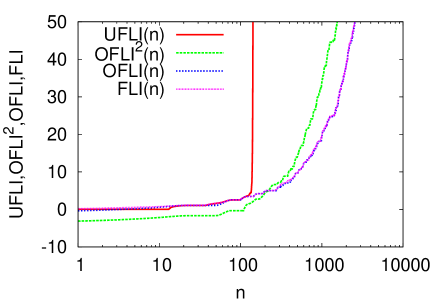
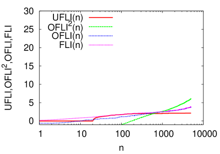
Figure 1: Point A. A time evolution of UFLI, OFLI², OFLI and FLI in a chaos domain. The common logarithm is used to calculate UFLI, OFLI², OFLI and FLI.

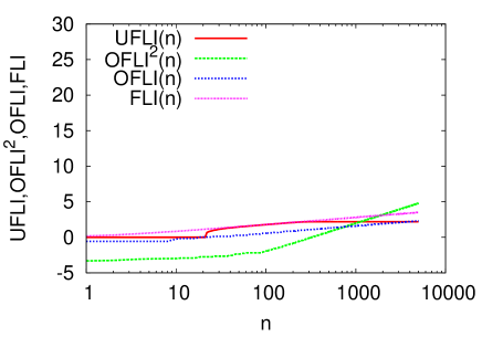
Figure 2: Point B. A time evolution of UFLI, OFLI², OFLI and FLI in a KAM torus domain. The common logarithm is used to calculate UFLI, OFLI², OFLI and FLI.

Figure 3: Point C. A time evolution of UFLI, OFLI², OFLI and FLI in a resonant torus domain. The common logarithm is used to calculate UFLI, OFLI², OFLI and FLI.

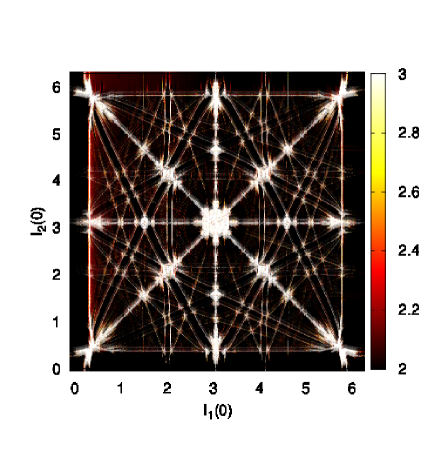
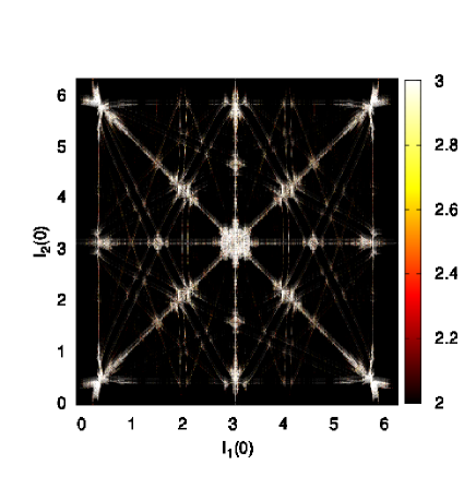
Figure 4: A digaram of UFLI for Froeschlé map with $\varepsilon=0.6$ at $n=200$. The common logarithm is used to calculate UFLI.

Figure 5: A diagram of OFLI² for Froeschlé map with $\varepsilon=0.6$ at $n=200$. The common logarithm is used to calculate OFLI².

According to Figs. 3, 3 and 3, our proposed UFLI performs much better compared to OFLI², OFLI and FLI. Figures 5 and 5 show diagrams of UFLI and OFLI² for Froeschlé map with $\varepsilon=0.6$ at $n=200$ whose initial condition is $\theta_{1}=\theta_{2}=0$. UFLI can show Arnold web, a structure consists of resonant lines more clearly than OFLI². According to Ref. Froeschle06 , this map behaves differently as a magnitude of $\varepsilon$. It is known in Ref. Froeschle06 that , Arnold diffusion occurs when $\varepsilon\leq 0.9$ and Chirikov diffusion occurs when $\varepsilon\geq 1.3$. Here, we apply UFLI to detect a change between these diffusion regime. We compare variations of UFLI and OFLI² v.s. $\varepsilon$. One thousand initial points are chosen near $(I_{1},I_{2})=(\pi/2,\pi/2)$. Figure 7 shows ensemble average of UFLI$(50)$ v.s. the parameter $\varepsilon$ change and Fig. 7 shows the counterpart of OFLI${}^{2}(50)$, OFLI(50) and FLI(50) instead of UFLI$(50)$. Figure 7 shows that UFLI loses smoothness in $\varepsilon\geq 0.9$ and distinguishes a transition between the two regimes (Arnold diffusion and Chirikov diffusion) of Froeschlé map although OFLI² and the other existing detectors such as FLI cannot detect any transition in Fig. 7. We define Lyapunov time $T_{L}$ and the macroscopic instability time $T_{I}$. In Arnold diffusion, $T_{I}\sim\exp\left(T_{L}\right)$ while in Chirikov diffusion, $T_{I}$ is order of polynomial for $T_{L}$ Morbidelli . Then, it is important to detect the point of $\varepsilon$ around which diffusion type changes.

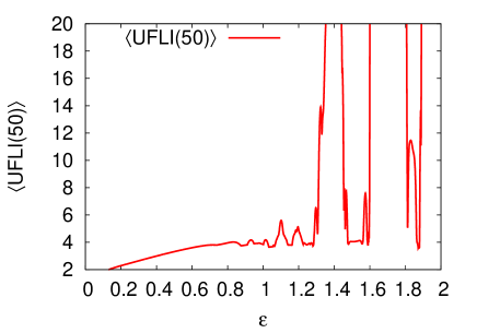
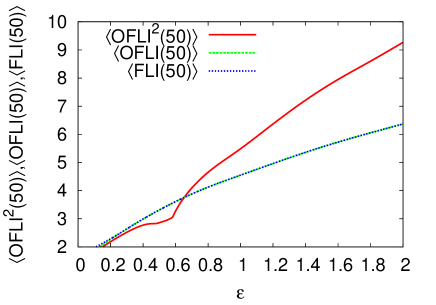
Figure 6: The ensemble average of UFLI$(50)$ v.s. $\varepsilon$. The common logarithm is used to calculate UFLI.

Figure 7: The ensemble average of OFLI${}^{2}(50)$, OFLI(50) and FLI(50) v.s. $\varepsilon$. The common logarithm is used to calculate OFLI².

According to the result above, our proposed UFLI chaos detector is very powerful to detect chaoticity of systems with relatively small Lyapunov exponents more rapidly and clearly than FLI, OFLI and OFLI². In addition to this, UFLI can also detect a sharp change of the diffusion regime between Arnold diffusion and Chirikov diffusion although OFLI² and the other existing indicators cannot detect any transition.

Log Fast Lyapunov Indicator

Here, we investigate further to chaotic systems with zero Lyapunov exponent. In generally, a positive Lyapunov exponent shows a existence of exponential growth of a variation between two close orbits. A positive value of Lyapunov exponent is used as an indicator of chaoticity. Even though the value of Lyapunov exponent is zero, behavior on torus and sub-exponential behavior with zero Lyapunov exponent are different. Thus, we propose another new indicator to distinguish them. In this section, Log Fast Lyapunov Indicator (LFLI)

$$\mbox{LFLI}(n)\equiv\log\left[\sup_{0<i\leq n}\log\left(\frac{\left\|D\bm{f}(\bm{x}_{i})\bm{w}_{i}\right\|}{\left\|\bm{w}_{0}\right\|}\right)\right]$$ (27)

is proposed to characterize sub-exponential behaviors. Here, $\bm{w}_{0},\bm{w}_{i},D\bm{f}(\bm{x}_{i})$ are an initial variational vetor, a variational vector at $n=i$ and a Jacobian of $\bm{f}(\bm{x}_{i})$ respectively. If infinite ergodic systems behave sub-exponentially Akimono , the time evolution of LFLI grows linearly with slope smaller than unity. If systems have a positive Lyapunov exponent, the slope is unity. We apply LFLI to the Boole transformation and the $S$-unimodal function in the following section.

Boole transformation

Here, the Boole transformation $T:\mathbb{R}\to\mathbb{R}$ is defined by

$$x_{n+1}=T(x_{n})\equiv x_{n}-\frac{1}{x_{n}}.$$ (28)

It is known that the Boole transformation is ergodic and preserves the Lebesgue measure Adler . The Boole transformation is an infinite ergodic system and the following equation is known to hold

$$\lim_{n\to\infty}\frac{1}{n}\sum_{k=1}^{n}f(T^{k}x)=0,$$ (29)

$$\mbox{ a.e. }x\in\mathbb{R},~{}{}^{\forall}\!f\in L^{1}(\mu),$$

where $\mu$ is the invariant measure for the probability preserving Boole transformation $T$ Aaronson97 . By substituting $f(T^{k}x)=\log|T^{\prime}(x_{k})|$, we know that the a value of Lyapunov exponent of Boole transformation is zero. However, it is known that the dynamical system behaves sub-exponentially Akimono . Namely, its orbital expansion rate $\Delta$ grows $\Delta\sim\exp(t^{\frac{1}{2}})$. By using the LFLI, we can find a power index. To compare with the Boole transformation, we consider the following generalized Boole transformations

$$x_{n+1}=T_{\alpha,~{}\beta}(x_{n})\equiv\alpha x_{n}-\frac{\beta}{x_{n}},$$ (30)

$$0<\alpha<1,0<\beta,$$

which are known to have non-negative Lyapunov exponent Umeno

$$\lambda=\log\left(1+2\sqrt{\alpha(1-\alpha)}\right).$$ (31)

We put $\beta=\alpha$ here for simplicity, because $\beta$ doesn’t affect on the Lyapunov exponent $\lambda$. Figure 8 shows ensemble averages of the time evolution of LFLI for the Boole transformation and the generalized Boole transformations with $\alpha=0.99995$ whose three hundred initial points are chosen near a point $x=11.7$. Here, the initial condition is $\bm{w}(0)=0.00000000000000000001$ and the float 128 precision is used to calculate LFLI.

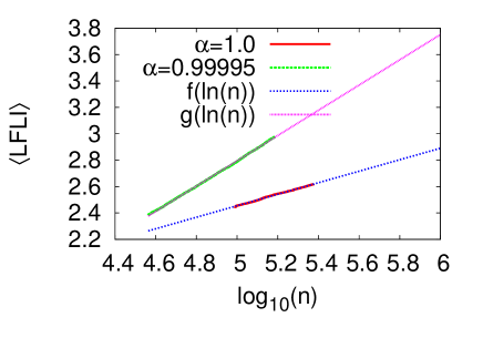
Figure 8: The ensemble average of the time evolution of LFLI of Boole transformation and generalized Boole transformation. The common logarithm is used to calculate LFLI.

In Fig. 8, the $f(\ln(n))$ and $g(\ln(n))$ are linear approximations of the ensemble averages of the Boole transformation and the generalized Boole transformations respectively. The slopes of $f(\ln(n))$ and $g(\ln(n))$ are about $0.436$ and $0.957$ respectively. These results indicate that our proposed LFLI is very powerful to find a power index for sub-exponential behavior.

$S$-unimodal function

$S$-unimodal function Thaler83 is defined by

$$X_{n+1}=T_{S}(X_{n})=\frac{1-5X_{n}^{2}}{1+3X_{n}^{2}},\ X_{n}\in[-1,1].$$ (32)

$S$-unimodal function has an infinite measure whose density function is

$$\rho(X)=\frac{1}{(1+X)\sqrt{1-X^{2}}}.$$ (33)

According to Ref. Thaler83 , orbit expansion rate of $S$-unimodal function is $\Delta\sim\exp(n^{\frac{1}{2}})$.

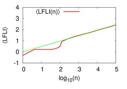
Figure 9: The time evolution of ensemble average of LFLI of the $S$-unmodal function. A slape of linear approximation for LFLI is about 0.486. The common logarithm is used to calculate LFLI.

Figure 9 shows the ensemble average of the time evolution of LFLI for the $S$-unmodal function whose one thousand initial points are chosen near a point $X=e^{-1}$. Here, the initial condition is $\bm{w}(0)=\exp(-20)$ and the float 128 precision is used to calculate LFLI.

Conclusion

We propose two chaos indicators Ultra Fast Lyapunov Indicator (UFLI) and Log Fast Lyapunov Indicator (LFLI). It is found that UFLI can detect chaoticity more rapidly than OFLI², OFLI and FLI and the only UFLI can detect a sharp change between Arnold diffusion and Chirikov diffusion regimes, that has not been detected by the existing methods such as OFLI². LFLI can measure a power index of a sub-exponential system. In particular, LFLI firstly characterizes chaoticity of systems which have zero Lyapunov exponent which has been regarded as non-chaotic systems. Such detectors UFLI and LFLI proposed here are very promising to detect chaoticity of experimental data of intrinsically weakly chaotic systems.

References

- (1) C. Froeschlé, R. Gonczi, and E. Lega, Planetary and space science 45, 881 (1997).
- (2) G. J. Sussman and J. Wisdom, Science 257, 56 (1992).
- (3) C. Froeschlé, E. Lega, and R. Gonczi, Celestial Mechanics and Dynamical Astronomy 67, 41 (1997).
- (4) M. Guzzo, E. Lega, and C. Froeschlé, Physica D 163, 1 (2002).
- (5) M. Fouchard, E. Lega, Chistiane Froeschlé, and Claude Froeschlé, Modern Celestial Mechanics: From Theory to Applications, (Springer, Netherlands, 2002).
- (6) R. Barrio., Chaos, Solitons and Fractals 25, 711 (2005).
- (7) T. Akimoto and Y. Aizawa, Chaos: An Interdisciplinary Journal of Nonlinear Science 20, 033110 (2010).
- (8) T. Akimoto, M. Nakagawa, S. Shinkai, and Y. Aizawa, Phy. Rev. E 91, 012926 (2015).
- (9) J. Aaronson, An Introduction to Infinite Ergodic Theory, (American Mathematical Society, Province, 1997).
- (10) R. Adler and B. Weiss, Israel Journal of Mathematics 16, 263 (1973).
- (11) M. Thaler, Israel Journal of Mathematics 46, 67 (1983).
- (12) U. Dressler and J. Farmer, Physica D: Nonlinear Phenomena 59, 365 (1992).
- (13) T. Taylor, Nonlinearity 6, 369 (1993).
- (14) C. Froeschlé, M. Guzzo, and E. Lega, Science 289, 2108 (2000).
- (15) C. Froeschlé, M. Guzzo, and E. Lega, A Comparison of the Dynamical Evolution of Planetary Systems, (Springer, Netherlands, 2005).
- (16) C. Froeschlé, E. Lega, and M. Guzzo, Celestial Mechanics and Dynamical Astronomy 95, 141 (2006).
- (17) A. Morbidelli and C. Froeschlé, Celestial Mechanics and Dynamical Astronomy 63, 227 (1996).
- (18) K. Umeno and K. Okubo, Exact Lyapunov exponent of generalized Boole transformation, Preprint, 2015.