ACCAMS
Additive Co-Clustering to Approximate Matrices Succinctly

Abstract

Matrix completion and approximation are popular tools to capture a user’s preferences for recommendation and to approximate missing data. Instead of using low-rank factorization we take a drastically different approach, based on the simple insight that an additive model of co-clusterings allows one to approximate matrices efficiently. This allows us to build a concise model that, per bit of model learned, significantly beats all factorization approaches to matrix approximation. Even more surprisingly, we find that summing over small co-clusterings is more effective in modeling matrices than classic co-clustering, which uses just one large partitioning of the matrix.

Following Occam’s razor principle suggests that the simple structure induced by our model better captures the latent preferences and decision making processes present in the real world than classic co-clustering or matrix factorization. We provide an iterative minimization algorithm, a collapsed Gibbs sampler, theoretical guarantees for matrix approximation, and excellent empirical evidence for the efficacy of our approach. We achieve state-of-the-art results on the Netflix problem with a fraction of the model complexity.

1 Introduction

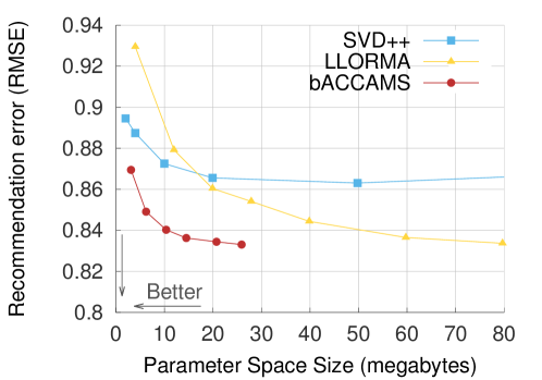
Figure 1: Accuracy of ACCAMS on Netflix, compared to [11] and [14]. Note that our model achieves state of the art accuracy at a fraction of the model size.

Given users’ ratings of movies or products, how can we model a user’s preferences for different types of items and recommend other items that the user will like? This problem, often referred to as the Netflix problem, has generated a flurry of research in collaborative filtering, with a variety of proposed matrix factorization models and inference methods. Top recommendation systems have used thousands of factors per item and per user, as was the case in the winning submissions in the Netflix prize [11]. Recent state-of-the-art methods have relied on learning even larger, more complex factorization models, often taking nontrivial combinations of multiple submodels [17, 14]. Such complex models use large amounts of memory, are increasingly difficult to interpret, and are often difficult integrate into larger systems.

1.1 Linear combinations of attributes

Our approach is drastically different from previous collaborative filtering research. Rather than start with the assumptions of a matrix factorization model, we make co-clustering effective for high quality matrix completion and approximation. Co-clustering has been well studied [2, 23] but was not previously competitive in large behavior modeling and matrix completion problems. To achieve state of the art results, we use an additive model of simple co-clusterings that we call stencils, rather than building a large single co-clustering. The result is a model that is conceptually simple, has a small parameter space, has interpretable structure, and achieves the best published accuracy for matrix completion on Netflix, as seen in Figure 1.

Using a linear combination of co-clusterings corresponds to a rather different interpretation of user preferences and movie properties. Matrix factorization assumes that a movie preference is based on a weighted sum of preferences for different genres, with the movie properties being represented in vectorial form. For instance, if a user likes comedies but not romantic movies, then a romantic comedy may have a predicted neutral 3-star rating.

Co-clustering on the other hand assumes there exists some “correct” partitioning of movies (and users). For instance, a user might be part of a group that likes all comedies but does not like romantic movies. Correspondingly, all romantic comedies might be aggregated into a cluster, possibly partitioned further into PG-13 rated, or R-rated romantic comedies. This quickly leads to a combinatorial explosion.

By taking a linear combination of co-clusterings we benefit from both perspectives: there is no single correct partitioning of movies and users; however, we can use the membership in several independent groups to encode the factorial nature of attributes without incurring the cost of a necessarily high-dimensional model of matrix factorization. For instance, a movie may be {funny, sad, thoughtful}, it might have a certain age rating, it might be an {action, romantic, thriller, documentary, family} movie, it might be shot in a certain visual style, and by a certain group of actors. By taking linear combinations of co-clusterings we can take these attributes into account.

1.2 Stencils

The mathematical challenge that motivated this work is that, in order to encode a rank-$k$ matrix by a factorization, we need $k$ numbers per row (and column) respectively. With linear combinations of stencils, on the other hand, we only need $\log_{2}k$ bits per row (and column) plus $O(k^{2})$ floating point numbers regardless of the size of the matrix.

We denote by a stencil a small $k\times k$ template of a matrix and its mapping to the row and column vectors respectively. This is best understood by the example below: assume that we have two simple stencils containing $3\times 3$ and $3\times 2$ co-clusterings. Their linear combination yields a rather nontrivial $9\times 9$ matrix of rank $5$.

In contrast, classic co-clustering would require a $(3\cdot 3)\times(3\cdot 2)$ partitioning to match this structure. When we have $s$ stencils of size $k\times k$, this requires a $k^{s}\times k^{s}$ partitioning.

By design our model has a parameter space that is an order of magnitude smaller than competing methods, requiring only $s\log_{2}k$ bits per user and per movie and $sk^{2}$ floating point numbers, where $k$ is generally quite small. This is computationally advantageous of course, but also demonstrates that our modeling assumptions better match real world structure of human decision making.

Finding succinct models for binary matrices, e.g. by minimizing the minimum description (MDL), has been the focus of significant research and valuable results in the data mining community [15, 12]. That said, these models are quite different. To the best of our knowledge, ours is the first work aimed at finding a parsimonious model for general (real-valued) matrix completion and approximation.

1.3 Contributions

Our paper makes a number of contributions to the problem of finding sparse representations of matrices.

• We present ACCAMS, an iterative $k$-means style algorithm that minimizes the approximation error by backfitting the residuals of previous approximations.

• We provide linear approximation rates exploiting the geometry of rows and columns of rating matrix via bounds on the metric entropy of Banach spaces.

• We present a generative Bayesian non-parametric model and devise a collapsed Gibbs sampling algorithm, bACCAMS, for efficient inference.

• Experiments confirm the efficacy of our approach, offering the best published results for matrix completion on Netflix, an interpretable hierarchy of content, and succinct matrix approximations for ratings, image, and network data.

We believe that these contributions offer a promising new direction for behavior modeling and matrix approximation.

Outline. We begin by discussing related work from recommendation systems, non-parametric Bayesian models, co-clustering, and minimum description length. We subsequently introduce the simple $k$-means style co-clustering and its approximation properties in Section 3. Subsequently, in Section 4.1 we define our Bayesian co-clustering model and collapsed Gibbs sampler for a single stencil. In Section 4.5 we extend our Bayesian model to multiple stencils. Section 5 reports our experimental results and we conclude with a discussion of future directions for the work.

2 Related Work

Recommender Systems. Probably the closest to our work is the variety of research on behavior modeling and recommendation. Matrix factorization approaches, such as Koren’s SVD++ [10], have enjoyed great success in recommender systems. Recent models such as DFC [17] and LLORMA [14] have focused on using ensembles of factorizations to exploit local structure.

More closely related to our model are Bayesian non-parametric approaches. For instance, [7, 6] use the Indian Buffet Process (IBP) for recommendation. In doing so they assume that each user (and movie) has certain preferential binary attributes. It can be seen as an extreme case of ACCAMS where the cluster size $k=2$, while using a somewhat different strategy to handle cluster assignment and overall similarity within a cluster. Following a similar intuition as ACCAMS but different perspective and focus, [19] extended the IBP to handle $k>2$ for link prediction tasks on binary graphs. Our work differs in its focus on general, real-valued matrices, its application of co-clustering, and its significantly simpler parameterization.

A co-clustering approach to recommendation was proposed by [3]. This model uses co-clustering to allow for sharing of strength within each group. However, it does not overcome the rank-$k$ problem, i.e. while clustering reduces intra-cluster variance and improves generalization, it does not increase the rank beyond what a simple factorization model is capable of doing. Finally, [21] proposed a factorization model based on a Dirichlet process over users and columns. All these models are closely related to the mixed-membership stochastic blockmodels of [1].

Co-clustering. It was was originally used primarily for understanding the clustering of rows and columns of a matrix rather than for matrix approximation or completion [9]. This formulation was well suited for biological tasks, but it computationally evolved to cover a wider variety of objectives [2]. [20] defined a soft co-clustering objective akin to a factorization model. Recent work has defined a Bayesian model for co-clustering focused on matrix modeling [23]. [27] focuses on exploiting co-clustering ensembles, but do so by finding a single consensus co-clustering. As far as we know, ours is the first work to use an additive combination of co-clusterings.

Matrix Approximation. There exists a large body of work on matrix approximation in the theoretical computer science community. They focus mainly on efficient low-rank approximations, e.g. by projection or by interpolation. Examples of the projection based strategy are [8, 4]. Essentially one aims to find a general low-rank approximation of the matrix, as is common in most recommender models.

A more parsimonious strategy is to seek interpolative decompositions. There one aims to approximate columns of a matrix by a linear combination of a subset of other columns [16]. Nonetheless this requires us to store at least one, possibly more scaling coefficients per column. Also note the focus on column interpolations — this can easily be extended to row and column interpolations, simply by first performing a row interpolation and then interpolating the columns. To the best of our knowledge, the problem of approximating matrices with piecewise constant block matrices as we propose here is not the focus of research in TCS.

Succinct modeling. The data mining community has focused on finding succinct models of data, often directly optimizing the model size described by the minimum description language (MDL) principle [22]. Finding effective ways to compress real world data allows for better modeling and understanding of the datasets. This approach has led to valuable results in pattern and item-set mining [26, 15] as well as graph summarization [12]. However, these approaches typically focus on modeling databases of discrete items rather than real-valued datasets with missing values.

3 Matrix Approximation

Before delving into the details of Bayesian Non-parametrics we begin with an optimization view of ACCAMS.

3.1 Model

Key to our model is the notion of a stencil, an extremely easy to represent block-wise constant rank-$k$ matrix.

Definition 1 (Stencil)

A stencil $S(T,c,d)$ is a matrix $S\in\mathbb{R}^{m\times n}$ with the property that $S_{ij}=T_{c_{i},d_{j}}$ for a template $T\in\mathbb{R}^{k_{m}\times k_{n}}$ and discrete index vectors $c\in\left\{1,\ldots,k_{m}\right\}^{m}$ and $d\in\left\{1,\ldots,k_{n}\right\}^{n}$ respectively.

Given a matrix $M\in\mathbb{R}^{m\times n}$ it is now our goal to find a stencil $S(T,c,d)$ such that the approximation error $M-S(T,c,d)$ is small while simultaneously the cost for storing $T,c,d$ is small. In the context of the example above, the $9\times 9$ matrix is given by the sum of two stencils, one of size $3\times 3$ and one of size $3\times 2$. This already indicates that we may require more than one stencil for efficient approximation. In general, our model will be such as to solve

$$\operatorname*{\mathrm{minimize}}_{\left\{T^{l},c^{l},d^{l}\right\}}\left\|M-\sum_{l=1}^{s}S(T^{l},c^{l},d^{l})\right\|^{2}_{\mathrm{Frob}}$$ (1)

That is, we would like to find an additive model of $s$ stencils that minimizes the approximation error to $M$. Such an expansion affords efficient compression using a trivial codebook, as can be seen below.

Lemma 2 (Compression)

The stencil $S(T,c,d)$ can be
stored at $\epsilon$ element-wise accuracy at no more cost than

$$O(m\log_{2}k_{m}+n\log_{2}k_{n}+k_{m}k_{n}\log_{2}\epsilon^{-1}\left\|T\right\|_{\infty}).$$

Proof.

This follows directly from the construction. Storing the vector $c$ costs at most $m\log_{2}k_{m}$ bits if we assume a uniform code (this also holds for $d$). When storing $T$ approximately, we must not quantize at a level of the approximation error or higher. Hence, a simplistic means of encoding the dynamic range requires $\log_{2}\left\|T\right\|_{\infty}/\epsilon$ bit, which is used on a per-element basis in $T$. ∎

Note that considerably better codes may exist whenever the entropy of $c$ is less than $\log_{2}k_{m}$ (likewise for $d$). Nonetheless, even the crude $\log_{2}k_{m}$ bound is already much better than what can be accomplished by a low-rank factorization.

Obviously, given $M$, it is our goal to find such stencils $S(T,c,d)$ with good approximation properties. Unfortunately, finding linear combinations of co-clusterings is as hard as co-clustering: assume that we are given all but one stencil of the optimal solution. In this case our problem reduces to co-clustering as its subproblem, which is NP-hard.

3.2 Algorithm

We consider a simple iterative procedure in which stencils are computed one at a time, using the residuals as input. The inner loop consists of a simple algorithm that is reminiscent of $k$-means clustering. It proceeds in two stages. Without loss of generality we assume that we have more rows than columns, i.e. $M\in\mathbb{R}^{m\times n}$ with $m\geq n$.

Row clustering. We first perform $k$-means clustering of the rows. That is, we aim to find an approximation of $M$ that replaces all rows by a small subset thereof. Note that this is more stringent than the interpolative approximations of matrices which only require us to find a set of rows which will form a (possibly sparse) basis for all other rows.

Algorithm 1 RowClustering

0:  matrix $M$, row clusters $k_{m}$

  Draw $k_{m}$ rows from $M$ at random without replacement and copy them to $\left\{v_{1},\ldots,v_{k_{m}}\right\}$.

  $t\leftarrow 0\in\mathbb{R}^{k_{m}}$ and $w\leftarrow 0\in\mathbb{R}^{k_{m}\times n}$

  while not converged do

     for $i=1$ to $m$ do

        $c_{i}\leftarrow\operatorname*{\mathrm{argmin}}_{j}\left\|M_{i:}-v_{j}\right\|_{2}^{2}$ {Find center}

        $t_{c_{i}}\leftarrow t_{c_{i}}+1$ {Increment cluster count}

        $w_{c_{i}}\leftarrow w_{c_{i}}+M_{i:}$ {Increment statistics}

     end for

     for $i=1$ to $a$ do

        $v_{i}\leftarrow w_{i}/t_{i}$ {New cluster center}

        $l_{i}\leftarrow t_{i}$ and $t_{i}\leftarrow 0$ {Cluster counts}

        $w_{i}\leftarrow(0,\ldots 0)\in\mathbb{R}^{n}$ {Reset statistics}

     end for

  end while

  return  clusters $\left\{v_{1},\ldots v_{k_{m}}\right\}$, IDs $c$, counts $l$

Algorithm 1 is essentially $k$-means clustering on the rows of $M$. Once we have this, we now cluster the columns of the new matrix in an analogous manner. The only difference is that the approximation needs to be particularly good for row clusters that occur frequently. Consequently the approximation measure $\left\|M_{i:}-v_{j}\right\|_{2}^{2}$ is replaced by the Mahalanobis distance. That is, the only substantial difference to Algorithm 1 is that now we use the assignment

$$d_{i}\leftarrow\operatorname*{\mathrm{argmin}}_{j}\left(V_{:i}-w_{j}\right)^{\top}D\left(V_{:i}-w_{j}\right)$$ (2)

where $V\in\mathbb{R}^{k_{m}\times n}$ is the matrix obtained by stacking $V_{i:}=v_{i}$ and $D$ is the diagonal matrix of counts, i.e. $D_{ii}=l_{i}$.

Missing entries. In many cases, however, $M$ itself is incomplete. This can be addressed quite easily by replacing the assignment $\operatorname*{\mathrm{argmin}}_{j}\left\|M_{i:}-v_{j}\right\|^{2}_{2}$ by

$$c_{i}\leftarrow\operatorname*{\mathrm{argmin}}_{j}\sum_{l:(i,l)\in M}\left(M_{il}-v_{jl}\right)^{2}$$ (3)

where we used $(i,l)\in M$ as a shorthand for the existing entries in $M$. In finding a good cluster for the row $M_{il}$ we restrict ourselves to the coordinates in $v_{j}$ where $M_{i:}$ exists.

Likewise, for the purpose of obtaining the column clusters, we now need to keep track for each coordinate in $V$ how many elements in $M$ contributed to it. Correspondingly denote by $t_{ej}:=\sum_{(e,j)\in M:c_{e}=i}1$ the number of entries mapped into coordinate $V_{ej}$. Then the assignment for column clusters is obtained via

$$d_{j}\leftarrow\operatorname*{\mathrm{argmin}}_{l}\sum_{i}\left(V_{lj}-w_{lj}\right)^{2}t_{lj}$$ (4)

and likewise the averages are now per-coordinate according to the counts for both $v$ and $w$.

Backfitting. The outcome of row and column clustering is a stencil $S(T,c,d)$ consisting of the clusters obtained by first row and then column clustering and of the assignment vectors $c$ and $d$ once the process is complete. It may be desirable to alternate between row and column clustering for further refinement. Since each step can only reduce the objective function further and the state space of $(c,d)$ is discrete, convergence to a local minimum is assured, with the same caveat on solution quality as in $k$-means clustering. The last step is to take the residual $M-S(T,c,d)$ and use it as the starting point of a new approximation round.

Algorithm 2 Matrix Approximation

0:  matrix $M$, clusters $k_{m},k_{n}$, max stencils $s$

  for $\mathrm{iter}=1$ to $s$ do

     $(V,c,l_{\mathrm{row}})\leftarrow\mathrm{RowClustering}(M,k_{a})$

     $(S,d,l_{\mathrm{col}})\leftarrow\mathrm{ColumnClustering}(V,b,\mathrm{diag}(l_{\mathrm{row}}))$

     for all $i,j\in\left\{1,\ldots k_{m}\right\}\times\left\{1,\ldots k_{n}\right\}$ do

        $T_{ij}\leftarrow\mathrm{mean}\left\{M_{ef}|c_{e}=i\text{ and }d_{f}=j\right\}$

     end for

     $M\leftarrow M-S(T,c,d)$ and back up $(T,c,d)$

  end for

Essentially the last stage is used to ensure that the stencil has minimum approximation error given the partitioning. This procedure is repeatedly invoked on the residuals to minimize the loss. The result is an additive model of co-clusterings.

3.3 Approximation Guarantees

A key question is how well any given matrix $M$ can be approximated by an appropriate stencil. For the sake of simplicity we limit ourselves to the case where all entries of the matrix are observed. We use covering numbers and spectral properties of $M$ to obtain approximation guarantees.

Definition 3 (Covering Number)

Denote by $\mathcal{B}$ a Banach Space. Then for any given set $B\in\mathcal{B}$ the covering number $\mathcal{N}_{\epsilon}(B)$ is given by the set of points $\left\{b_{1},\ldots b_{\mathcal{N}_{\epsilon}(B)}\right\}$ such that for any $b\in B$ there exists some $b_{j}$ with $\left\|b-b_{j}\right\|\leq\epsilon$.

Of particular interest for us are covering numbers $\mathcal{N}_{\epsilon}$ of unit balls and their functional inverses $\epsilon_{n}$. The latter are referred to as entropy number and they quantify the approximation error incurred by using a cover of $n$ elements [24, Chapter 8]. A key tool for computing entropy numbers of scaling operators is the theorem of Gordon, König and Schütt [5], relating entropy numbers to singular values.

Theorem 4 (Entropy Numbers and Singular Values)

Denote by $D$ a diagonal scaling operator with $D:\ell_{p}\to\ell_{p}$ with scaling coefficients $\sigma_{i}\geq\sigma_{i+1}\geq 0$ for all $i$. Then for all $n\in\mathbb{N}$ the entropy number $\epsilon_{n}(D)$ is bounded via

$$\epsilon_{n}(D)\leq 6\sup_{j\in\mathbb{N}}\left(n^{-1}\prod_{i=1}^{j}\sigma_{i}\right)^{\frac{1}{j}}\leq 6\epsilon_{n}(D)$$ (5)

This means that if we have a matrix with rapidly decaying singular values, we only need to focus on the leading largest ones in order to approximate all elements in the space efficiently. Here the tradeoff between dimensionality and accuracy is obtained by using the harmonic mean.

Corollary 5 (Entropy Numbers of Unit Balls)

The covering number of a ball $\mathcal{B}$ of radius $r$ in $\ell_{2}^{d}$ is bounded by

$$rn^{-\frac{1}{d}}\leq\epsilon_{n}(\mathcal{B})\leq 6rn^{-\frac{1}{d}}.$$ (6)

Proof.

This follows directly from using the linear operator $x\to rx$ for $x\in\ell_{2}^{d}$. Here the scaling operator has eigenvalues $\sigma_{i}=r$ for all $1\leq i\leq d$ and $\sigma_{i}=0$ for $i>d$. The maximum in (5) is always $j=d$. ∎

The following theorem states that we can approximate $M$ up to a multiplicative constant at any step, provided that we pick a large enough clustering. It also means that we get linear convergence, i.e. convergence in $O(\log\epsilon)$ steps to $O(\epsilon)$ error, since the bound can be applied iteratively.

Theorem 6 (Approximation Guarantees)

Denote by $\sigma_{1},\ldots\sigma_{n}$ the singular values of $M$. Then using $l$ clusters for rows and columns respectively the matrix $M$ can be approximated with error at most

$$\left\|M-M^{\prime}\right\|_{\infty} \leq 2\left\|M\right\|^{\frac{1}{2}}\epsilon_{l}\left(\Sigma^{\frac{1}{2}}\right)$$

$$\left\|M-M^{\prime}\right\|_{2} \leq(\sqrt{m}+\sqrt{n})\left\|M\right\|^{\frac{1}{2}}\epsilon_{l}\left(\Sigma^{\frac{1}{2}}\right)$$

Here $\epsilon_{l}$ is given by Theorem 4 and Corollary 5 respectively.

Proof.

Using the singular value decomposition of $M$ into $M=U\Sigma V$ we can factorize $M=Q^{\top}R$ where $Q=\Sigma^{\frac{1}{2}}U$ and $R=\Sigma^{\frac{1}{2}}V$. By construction, the singular values of $Q$ and $R$ are $\Sigma^{\frac{1}{2}}$. We now cluster the rows of $Q$ and $R$ independently to obtain an approximation of $M$.

For $Q$ we know that its rows can be approximated by $l$ balls with error $\epsilon_{l}\left(\Sigma^{\frac{1}{2}}\right)$ as per Theorem 4. Also note that its row vectors are contained in the image of the unit ball under $Q$ — if they were not, project them onto the unit ball and the approximation error cannot increase since the targets are within the unit ball, too. Hence the $\epsilon_{l}$-cover of the latter also provides an approximation of the row-vectors of $Q$ by $Q^{\prime}$ with accuracy $\epsilon_{l}$, where $Q^{\prime}$ contains at most $l$ distinct rows. The same holds for the matrix $R$, as approximated by $R^{\prime}$. Hence we have

$$\left|M_{ij}-\left\langle Q_{i:}^{\prime},R_{j:}^{\prime}\right\rangle\right| =\left|\left\langle Q_{i:},R_{j:}\right\rangle-\left\langle Q_{i:}^{\prime},R_{j:}^{\prime}\right\rangle\right|$$

$$=\left|\left\langle Q_{i:}-Q_{i:}^{\prime},R_{j:}\right\rangle+\left\langle Q_{i:}^{\prime},R_{j:}-R_{j:}^{\prime}\right\rangle\right|$$

$$\leq\left\|Q_{i:}-Q_{i:}^{\prime}\right\|\left\|R_{j:}\right\|+\left\|Q_{i:}^{\prime}\right\|\left\|R_{j:}-R_{j:}^{\prime}\right\|$$

$$\leq 2\left\|M\right\|^{\frac{1}{2}}\epsilon_{l}\left(\Sigma^{\frac{1}{2}}\right)$$

This provides a pointwise approximation guarantee.If we only have a bound on the rank and on $\left\|M\right\|$, this yields

$$\left|M_{ij}-\left\langle q_{i},r_{j}\right\rangle\right|\leq 12\left\|M\right\|l^{\frac{1}{2d}}$$

Moreover, since each row in $Q$ and $R$ respectively will be approximated with residual bounded by $\epsilon_{l}$ we can bound $\left\|Q-Q^{\prime}\right\|\leq\sqrt{m}\epsilon_{l}$ and $\left\|R-R^{\prime}\right\|\leq\sqrt{n}\epsilon_{l}$ respectively. This yields a bound on the matrix norm of the residual via

$$\left\|\left[QR-Q^{\prime}R^{\prime}\right]x\right\| \leq\left\|Q(R-R^{\prime})x\right\|+\left\|(Q-Q^{\prime})R^{\prime}x\right\|$$

$$\leq(\sqrt{m}+\sqrt{n})\left\|M\right\|^{\frac{1}{2}}\epsilon_{l}\left(\Sigma^{\frac{1}{2}}\right)\left\|x\right\|$$

This bounds the matrix norm of the residual. ∎

Note that the above is an existence proof rather than a constructive prescription. However, by using the fact that set cover is a submodular problem [28], it follows that given $l$, we are able to obtain a near-optimal cover, thus leading to a constructive algorithm. Note, however, that the main purpose of the above analysis is to obtain theoretical upper bounds on the rate of convergence. In practice, the results can be considerably better, as we show in Section 5.

4 Generative Model

In the same manner as many risk minimization problems (e.g. penalized logistic regression) have a Bayesian counterpart (Gaussian Process classification) [18], we now devise a Bayesian counterpart to ACCAMS, which we will refer to as bACCAMS. We begin with the single stencil case in Section 4.1 and extend it to many stencils in Section 4.5.

Figure 2: Generative model for recommdnation and matrix approximation (bACCAMS). For each stencil, as indexed by $l$, row and cluster memberships $c^{l}$ and $d^{l}$ are drawn from a Chinese Restaurant Process. The values for the template $T^{l}$ are drawn from a Normal Distribution. The observed ratings $M_{um}$ are sums over the stencils $S(T^{l},c^{l},d^{l})$.

4.1 Co-Clustering with a Single Stencil

We begin with a simplistic model of co-clustering. It serves as the basic template for single-matrix inference. All subsequent steps use the same idea. In a nutshell, we assume that each user $u$ belongs to a particular cluster $c_{u}$ drawn from a Chinese Restaurant Process $\mathrm{CRP}(\alpha)$. Likewise, we assume that each movie $m$ belongs to some cluster $d_{m}$ drawn analogously from $\mathrm{CRP}(\beta)$. The scores of the matrix $M_{um}$ are obtained from a stencil $S(T,c,d)_{um}=T_{c_{u}d_{m}}$ with additive noise $\epsilon_{um}\sim\mathcal{N}(0,\sigma^{2})$. The stencil values $T_{cd}$ themselves are drawn from a normal distribution $\mathcal{N}(0,\tau^{2})$. In turn, the variances $\tau^{2}$ and $\sigma^{2}$ are obtained via a conjugate prior, i.e. the Inverse Gamma distribution.

This is an extremely simple model similar to [23], akin to a decision stump. The rationale for picking such a primitive model is that we will be combining linear combinations thereof to obtain a very flexible tool. The model is shown in Figure 2. For $l=1$ the formal definition is as follows:

$$c_{u} \sim\mathrm{CRP}(\alpha) d_{m} \sim\mathrm{CRP}(\beta)$$ (7a)

$$T_{cd} \sim\mathcal{N}(0,\tau^{2}) M_{um} \sim\mathcal{N}\left(T_{c_{u}d_{m}},\sigma^{2}\right)$$ (7b)

$$\tau^{2} \sim\mathrm{IG}(\gamma) \sigma^{2} \sim\mathrm{IG}(\eta)$$ (7c)

Recall that the Inverse Gamma distribution is given by

$$p(x|a,b) =b^{a}\Gamma^{-1}(a)x^{-a-1}e^{-\frac{b}{x}}$$ (8)

$$\text{and hence }p(\sigma^{2}|\eta_{a},\eta_{b}) =\eta_{b}^{\eta_{a}}\Gamma^{-1}(\eta_{a})\sigma^{-2(\eta_{a}+1)}e^{-\frac{\eta_{b}}{\sigma^{2}}}$$ (9)

Consequently the joint probability distribution over all scores, given the variances is given by

$$p\left(M,S(T,c,d)|\alpha,\beta,\sigma^{2},\tau^{2}\right)$$ (10)

$$= \mathrm{CRP}(c|\alpha)\mathrm{CRP}(d|\beta)\prod_{c,d}{\frac{1}{\sqrt{2\pi\tau^{2}}}}\exp\left(-\frac{T_{cd}^{2}}{2\tau^{2}}\right)\prod_{(u,m)}{\frac{1}{\sqrt{2\pi\sigma^{2}}}}\exp\left(-\frac{\left(M_{um}-T_{c_{u}d_{u}}\right)^{2}}{2\sigma^{2}}\right)$$

The idea is that each user and each movie are characterized by a simple cluster. Since we chose all priors to be conjugate to the likelihood terms, it is possible to collapse out the choice of $T_{cd}$. This is particularly useful as it allows us to accelerate the sampler considerably — now we only sample over the discrete random variables $c_{u},d_{m}$ indicating the cluster memberships for a particular user and movie. In other words, we obtain a closed form expression for $p(M,c,d|\alpha,\beta,\sigma^{2},\tau^{2})$. Moreover, $\sigma^{2}|S(T,c,d),\eta$ and $\tau^{2}|T,\gamma$ are both Inverse Gamma due to conjugacy, hence we can sample them efficiently after sampling $T$.

4.2 Inferring Clusters

In the following we discuss a partially collapsed Gibbs sampler (effectively we use a Rao-Blackwellization strategy when sampling cluster memberships) for efficient inference. We begin with the part of sampling $c|d,\alpha,\sigma^{2},\tau^{2}$.

Chinese Restaurant Process:

It is well known that for exponential families the conjugate distribution allows for collapsing by taking ratios between normalization coefficients with and without the additional sufficient statistics item. See e.g. [7, Appendix A] for a detailed derivation. Denote by $n_{i},m_{j}$ the number of users and movies belonging to clusters $i$ and $j$ respectively. Moreover, denote by $n$ and $m$ the total number of users and movies, and by $k_{n},k_{m}$ the number of clusters. In this case we can express

$$p(c|\alpha) =\alpha^{k_{n}}\left[\prod_{i=1}^{k_{n}}\Gamma(n_{i})\right]\frac{\Gamma(\alpha)}{\Gamma(\alpha+n)}$$

$$\text{and hence }p(c_{i}=t|c^{-i},\alpha) =\begin{cases}\frac{n_{t}^{-i}}{\alpha+n-1}&\text{ if $n_{t}^{-i}>0$}\\ \frac{\alpha}{\alpha+n-1}&\text{ otherwise}\end{cases}$$

An analogous expression is available for $p(d|\beta)$ and $p(d_{j}=t|d^{-j},\beta)$. Note that the superscript $\left[\cdot\right]^{-i}$ denotes that the $i$-th observation is left out when computing the statistic. Large values of $\alpha$ and $\beta$ encourage the formation of larger numbers of clusters. The collapsed expressions will be useful for Gibbs sampling.

Integrating out $T$:

For faster mixing we need to integrate out $T$ whenever we resample $c$ and $d$. As we shall see, this is easily accomplished by keeping simple linear statistics of the ratings. Moreover, by integrating out $T$ we avoid the problem of having to instantiate a new value whenever a new cluster is added.

For a given block $(c,d)$ with associated $T_{cd}$, the distribution of ratings is Gaussian with mean $0$ and with covariance matrix $\sigma^{2}\mathbf{1}+\tau^{2}11^{\top}$ (due to the independence of the variances and the additive nature of the normal distribution). Here we use $\mathbf{1}$ to denote the identity matrix and $1$ to denote the vector of all $1$. Denote by $n_{cd}$ the number of rating pairs $(u,m)$ for which $c_{u}=c$ and $d_{m}=d$. Moreover, denote by $M_{cd}$ the vector of associated ratings. Hence, the likelihood of the cluster block $(c,d)$, as observed in $M_{cd}$ is

$$p(M_{cd}|\sigma^{2},\tau^{2})=\frac{\exp\left[-\frac{1}{2}M_{cd}^{\top}\left[\sigma^{2}\mathbf{1}+\tau^{2}11^{\top}\right]^{-1}M_{cd}\right]}{(2\pi)^{\frac{n_{cd}}{2}}\left|\sigma^{2}\mathbf{1}+\tau^{2}11^{\top}\right|^{\frac{1}{2}}}$$

In computing the above expression we need to compute the determinant of a diagonal matrix with rank-1 update, and the inverse of said matrix. For the former, we use the matrix-determinant lemma, and for the latter, the Sherman-Morrison-Woodbury formula:

$$M_{cd}^{\top}\left[\sigma^{2}\mathbf{1}+\tau^{2}11^{\top}\right]^{-1}M_{cd} =\frac{1}{\sigma^{2}}\left\|M_{cd}\right\|^{2}-\frac{\tau^{2}}{\sigma^{2}}\cdot\frac{\left(1^{\top}M_{cd}\right)^{2}}{\sigma^{2}+n_{cd}\tau^{2}}$$

$$\log\left|\sigma^{2}\mathbf{1}+\tau^{2}11^{\top}\right| =(n_{cd}-1)\log\sigma^{2}+\log\left[\sigma^{2}+n_{cd}\tau^{2}\right]$$

This allows us to assess whether it is beneficial to assign a user $u$ or a movie $m$ to a different or a new cluster efficiently, since the only statistics involved in the operation are sums of residuals and of their squares.

This leads to a collapsed Gibbs-sampling algorithm. At each step we check how likelihoods change by assigning a movie (or user) to another cluster. We denote by $n_{cd}^{\prime}$ the new cluster count and by $M_{cd}^{\prime}$ the new set of residuals. Let

$$\Delta:={\textstyle\frac{n_{cd}^{\prime}-n_{cd}}{2}}\left[\log(2\pi)+\log\sigma^{2}\right]+\frac{1}{2\sigma^{2}}\left[\left\|M_{cd}^{\prime}\right\|^{2}-\left\|M_{cd}\right\|^{2}\right]$$

be a constant offset, in log-space, that only depends on the additional ratings that are added to a cluster. In other words, it is independent of the cluster that the additional scores are assigned to. Hence $\Delta$ can be safely ignored.

$$p(c_{u}=c|\cdot)\propto \frac{n_{c}^{-i}}{\alpha+n-1}\prod_{d}\left[\frac{\sigma^{2}+n_{cd}\tau^{2}}{\sigma^{2}+n_{cd}^{\prime}\tau^{2}}\right]^{\frac{1}{2}}\exp\left[\frac{\tau^{2}}{2\sigma^{2}}\sum_{d}\left[\frac{\left(1^{\top}M_{cd}^{\prime}\right)^{2}}{\sigma^{2}+n_{cd}^{\prime}\tau^{2}}-\frac{\left(1^{\top}M_{cd}\right)^{2}}{\sigma^{2}+n_{cd}\tau^{2}}\right]\right]$$ (11)

For a new cluster this can be simplified since there is no data, hence $n_{cd}=0$ and $M_{cd}=[]$.

$$p(c_{u}=c_{\mathrm{new}}|\cdot)\propto {\textstyle\frac{\alpha}{\alpha+n-1}}\prod_{d}\left[\textstyle\frac{\sigma^{2}}{\sigma^{2}+n_{cd}^{\prime}\tau^{2}}\right]^{\frac{1}{2}}\exp\left[{\textstyle\frac{\tau^{2}}{2\sigma^{2}}}\sum_{d}\textstyle\frac{\left(1^{\top}M_{cd}^{\prime}\right)^{2}}{\sigma^{2}+n_{cd}^{\prime}\tau^{2}}\right]$$ (12)

The above expression is fairly straightforward to compute: we only need to track $n_{cd}$, i.e. the number of ratings assigned to a particular (user cluster, movie cluster) combination and $1^{\top}M_{cd}$, i.e. the sum of the scores for this combination.

4.3 Inferring Variances

For the purpose of recommendation and for a subsequent combination of several matrices, we need to infer variances and instantiate the scores $T_{cd}$. By checking (10) we see that $T_{cd}|\mathrm{rest}$ is given by a normal distribution with parameters

$$T_{cd}|\mathrm{rest}\sim\mathcal{N}\left(\textstyle\frac{1^{\top}M_{cd}}{\rho n_{cd}},\frac{\sigma^{2}}{\rho n}\right)\text{ where }\rho=\left[1+\textstyle\frac{1}{n_{cd}}\frac{\sigma^{2}}{\tau^{2}}\right].$$ (13)

Note that the term $\rho$ plays the role of a classic shrinkage term just as in a James-Stein estimator. To sample $\sigma^{2}$ and $\tau^{2}$ we use the Inverse Gamma distribution of (8).

Denote by $E$ the total number of observed values in $M$. In this case, $\sigma^{2}$ is drawn from an Inverse Gamma prior with parameters $(\eta^{\prime}_{a},\eta^{\prime}_{b})$:

$$\eta^{\prime}_{a}\leftarrow\eta_{a}+\frac{E}{2}\text{ and }\eta^{\prime}_{b}\leftarrow\eta_{b}+\sum_{(u,m)}(M_{um}-T_{c_{u}d_{m}})^{2}.$$ (14)

Analogously, we draw $\tau^{2}$ from an Inverse Gamma with parameters

$$\gamma^{\prime}_{a}\leftarrow\gamma_{a}+\frac{k_{n}k_{m}}{2}\text{ and }\gamma^{\prime}_{b}\leftarrow\gamma_{b}+\sum_{c,d}T_{cd}^{2}$$ (15)

$k_{n}$ and $k_{m}$ denote the number of user and movie clusters.

4.4 Efficient Implementation

With these inference equations we can implement an efficient sampler, as seen in Algorithm 3. The key to efficient sampling is to cache the per-cluster sums of ratings $1^{\top}M_{cd}$. Then reassigning a user (or movie) to a different (or new) cluster is just a matter of checking the amount of change that this would effect. Hence each sampling pass costs $O(k_{n}\cdot k_{m}\cdot(n+m)+E)$ operations. It is linear in the number of ratings and of partitions.

Algorithm 3 StencilSampler

  Initialize row-index and column-index of data in $M$

  Initialize sum of squares $Q:=\sum_{(u,m)}M_{um}^{2}$

  Initialize statistics for each partition

$$n_{cd}:=\left\{(u,m):c_{u}=c,d_{m}=d\right\}\text{ and }l_{cd}:=\sum_{(u,m):c_{u}=c,d_{m}=d}M_{um}$$

  while sampler not converged do

     for all users $u$ do

        For all movie clusters $d$ compute the incremental changes

$$n_{ud}:=\left\{(u,m):d_{m}=d\right\}\text{ and }l_{ud}:=\sum_{(u,m):d_{m}=d}M_{um}$$

        Remove $u$ from their cluster $\displaystyle n_{c_{u}d}\leftarrow n_{c_{u}d}-n_{ud}$

        Remove $u$ from their cluster $\displaystyle l_{c_{u}d}\leftarrow l_{c_{u}d}-n_{ud}$

        Sample new user cluster $c_{u}$ using (11) and (12).

        Update statistics

$$n_{c_{u}d}\leftarrow n_{c_{u}d}+n_{ud}\text{ and }l_{c_{u}d}\leftarrow l_{c_{u}d}+n_{ud}$$

     end for

     for all movies $m$ do

        Sample movie cluster assignments analogously.

     end for

     for all $(c,d)$ cluster partitions do

        Resample $T_{cd}$ using (13) and the statistics $n_{cd},l_{cd}$.

     end for

     Resample $\sigma^{2}$ and $\tau^{2}$ via the Inverse Gamma distribution using (14) and (15).

  end while

Note that once $n_{ud}$ and $l_{ud}$ are available for all users (or all movies), it is cheap to perform additional sampling sweeps at comparably low cost. It is therefore beneficial to iterate over all users (or all movies) more than once, in particular in the initial stages of the algorithm. Also note that the algorithm can be used on datasets that are being streamed from disk, provided that an index and an inverted index of $M$ can be stored: we need to be able to traverse the data when ordered by users and when ordered by movies. It is thus compatible with solid state disks.

4.5 Additive Combinations of Stencils

If there was no penalty on the number of clusters it would be possible to approximate any matrix by a trivial model using as many clusters as we have rows and columns.

Lemma 7

Any matrix $M\in\mathbb{R}^{m\times n}$ has nonvanishing support in (10) regardless of $\sigma^{2}$.

Proof.

Since any partitionings of sets of size $m,n$ respectively have nonzero support, it follows that partitioning all rows and all columns into separate bins is possible. Hence, we can assign a different mean $\mu_{cd}$ to any entry $M_{um}$. ∎

Obviously, the CRP prior on $c$ and $d$ makes this highly unlikely. On the other hand, we want to retain the ability to fit a richer set of matrices than what can be effectively covered by piecewise constant block matrices. We take linear combinations of matrices, as introduced in Section 3.

As before, we enumerate the stencils by $S(T^{l},c^{l},d^{l})$. Correspondingly we now need to sample from a set of $S(T^{l},c^{l},d^{l})$ and $\tau^{2}$ per matrix. However, we keep the additive noise term $\mathcal{N}(0,\sigma^{2})$ unchanged. This is the model of Figure 2. The additivity of Gaussians renders makes inference easy:

$$M_{um}\sim\mathcal{N}\left(\sum_{l}S(T^{l},c^{l},d^{l}),\sigma^{2}\right).$$ (16)

Note, though, that estimating $S$ jointly for all indices $l$ is not tractable since various clusterings $(c^{l},d^{l})$ overlap and intersect with each other, hence the joint normal distribution over all variables would be expensive to factorize.

Algorithm 4 bACCAMS

  initialize residuals $\rho:=M$ and $T^{l}=0$

  while sampler not converged do

     for all stencils $l$ do

        Compute partial residuals $\rho\leftarrow\rho-S(T^{l},c^{l},d^{l})$

        Sample over $S(T^{l},c^{l},d^{l})$ using $\rho$ instead of $M$

        Update residuals with $\rho\leftarrow\rho+S(T^{l},c^{l},d^{l})$

     end for

  end while

Instead, we sample over one stencil at a time, as shown in Algorithm 4. This algorithm only requires repeated passes through the dataset. Moreover, it can be modified into a backfitting procedure by fitting one matrix at a time and then fixing the outcome. Capacity control can be enforced by modifying $\alpha$ and $\beta$ such that the probability of a new cluster decreases for larger $l$, i.e. by decreasing $\alpha$ and $\beta$. As a result following the analysis in the single stencil case, each sampling pass costs $O(s\cdot(k_{n}\cdot k_{m}\cdot(n+m)+E))$ operations where $s$ is the number of stencils. It is linear in the number of ratings, in the number of partitions and in the number of stencils.

5 Experiments

We evaluate our method based on its ability to perform matrix completion, matrix approximation and to give interpretable results. Here we describe our experimental setup and results on real world data, such as the Netflix ratings.

5.1 Implementation

We implemented both ACCAMS, the $k$-means-based algorithm, as well as bACCAMS, the Bayesian model. Unless specified otherwise, we run the RowClustering of Algorithm 1 for up to $T=50$ iterations. Our system can also iterate over the stencils multiple times, such that earlier stencils can be re-learned after we have learned later ones. In practice, we observe this only yields small gains in accuracy, hence we generally do not use it.

We implemented bACCAMS using Gibbs sampling (Section 4.5) and used the $k$-means algorithm ACCAMS for the initialization of each stencil. Following standard practice, we bound the range of $\sigma$ by $\sigma_{\rm max}$ from above. This rejection sampler avoids pathological cases. For the sake of simplicity, we set $k=k_{n}=k_{m}$ to be the maximum number of clusters that can be generated in each stencil. When inferring the cluster assignments for a given stencil, we run three iterations of the sampler before proceeding to the next stencil. As common in MCMC algorithms, we use a burn-in period of at least 30 iterations (each with three sub-iterations of sampling cluster assignments) and then average the predictions over many draws. Code for both ACCAMS and bACCAMS is available at http://alexbeutel.com/accams.

5.2 Experimental Setup

Netflix. We run our algorithms on data from a variety of domains. Our primary testing dataset is the ratings dataset from the Netflix contest. The dataset contains 100M ratings from 480k users and 17k movies. Following standard practice for testing recommendation accuracy, we average over three different random 90:10 splits for training and testing.

CMU Face Images. To test how well we can approximate arbitrary matrices, we use image data from the CMU Face Images dataset. It contains black and white images of 20 different people, each in 32 different positions, for a total of 640 images. Each image has $128\times 120$ pixel resolution; we flatten this into a matrix of $640\times 15360$, i.e. an image by pixel matrix.

AS Peering Graph. To assess our model’s ability to deal with graph data we consider the AS graph. It contains information on the peering information of 13,580 nodes. It thus creates a binary matrix of size $13,580\times 13,580$ with 37k edges. Since our algorithm is not designed to learn binary matrices, we treat the entries $\left\{0,1\right\}$ as real valued numbers.

Parameters. For all experiments, we set the hyperparameters in bACCAMS to $\alpha=\beta=10$, $\eta_{\alpha}=2$, $\eta_{\beta}=0.3$, $\gamma_{\alpha}=5$, and $\gamma_{\alpha}=0.3$. Depending on the task, we compare ACCAMS against SVD++ using the GraphChi [13] implementation, SVD from Matlab for full matrices, and previously reported state-of-the-art results.

Model complexity. Since our model is structurally quite different from factorization models, we compare them based on the number of bits in the model and prediction accuracy. For factorization models, we consider each factor to be a 32 bit float. Hence the complexity of a rank $R$ SVD++ model of $n$ users and $m$ movies is $32\cdot R(n+m)$ bits.

For ACCAMS with $s$ stencils and $k\times k$ co-clusters in each stencil, the cluster assignment for a given row or column is $\log_{2}k$ bits and each value in the stencil is a float. As such, the complexity of a model is $s((n+m)\log_{2}k+32\cdot k^{2})$ bits.

In calculating the parameter space size for LLORMA, we make the very conservative estimate that each row and column is on average part of two factorizations, even though the model contains more than 30 factorizations that each row and column could be part of.

5.3 Matrix Completion

Since the primary motivation of our model is collaborative filtering we begin by discussing results on the classic Netflix problem; accuracy is measured in RMSE. To avoid divergence we set $\sigma_{\rm max}=1$. We then vary both the number of clusters $k$ and the number of stencils $s$.

A summary of recent results as well as results using our method can be found in Table 1. Using GraphChi we run SVD++ on our data. We use the reported values from LLORMA [14] and DFC [17], which were obtained using the same protocol as reported here.

As can be seen in Table 1, bACCAMS achieves the best published result. We achieve this while using a very different model that is significantly simpler both conceptually and in terms of parameter space size. We also did not use any of the temporal and contextual variants that many other models use to incorporate prior knowledge.

As shown in Figure 1, we observe that per bit our model achieves much better accuracy at a fraction of the model size. In Figure 3(a) we compare different configurations of our algorithm. As can be seen, classic co-clustering quickly overfits the training data and provides a less fine-grained ability to improve prediction accuracy than ACCAMS. Since ACCAMS has no regularization, it too overfits the training data. By using a Bayesian model with bACCAMS, we do not overfit the training data and thus can use more stencils for prediction, greatly improving the prediction accuracy.

Method	Parameters	Size	Test RMSE
SVD++ [13]	$R=25$	49.8MB	0.8631
DFC-NYS [17]	Not reported		0.8486
DFC-PROJ [17]	Not reported		0.8411
LLORMA [14]	$R=1$	3.98MB	0.9295
LLORMA [14]	$R=5$, $a>30$	19.9MB	0.8604
LLORMA [14]	$R=10$, $a>30$	39.8MB	0.8444
LLORMA [14]	$R=20$, $a>30$	79.7MB	0.8337
ACCAMS	$k=10$, $s=13$	2.69MB	0.8780
ACCAMS	$k=100$, $s=5$	2.27MB	0.8759
bACCAMS	$k=10$, $s=50$	10.4MB	0.8403
bACCAMS	$k=10$, $s=70$	14.5MB	0.8363
bACCAMS	$k=10$, $s=125$	25.9MB	0.8331

Table 1: bACCAMS achieves an accuracy for matrix completion on Netflix better than or on-par with the best published results, while having a parameter space a fraction of the size of other methods. $a$ denotes the number of anchor points for LLORMA and sizes listed are the parameter space size.

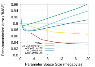
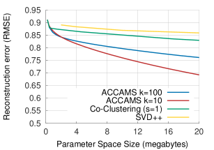
(a) Netflix Prediction	(b) Netflix Training Error
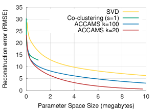
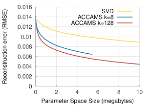
(c) Faces	(d) AS Graph

Figure 3: On images, ratings, and binary graphs, ACCAMS approximates the matrix more efficiently than SVD, SVD++, or classic co-clustering.

5.4 Matrix Approximation

In addition to matrix completion, it is valuable to be able to approximate matrices well, especially for dimensionality reduction tasks. To test the ability of ACCAMS to model matrix data we analyze both how well our model fits the training data from the Netflix tests above as well as on image data from the CMU Faces dataset and a binary matrix from the AS peering graph. (Note, for Netflix we now use the training data from one split of the dataset.) For each of these of datasets we compare to the SVD (or SVD++ to handle missing values). We also use our algorithm to perform classic co-clustering by setting $s=1$ and varying $k$.

As can be seen in Figure 3(b-d), ACCAMS models the matrices from all three domains much more compactly than SVD (or SVD++ in the case of the Netflix matrix, which contains missing values). In particular, we observe on the CMU Faces matrix that ACCAMS uses in some cases under $\frac{1}{4}$ of the bits as SVD for the same quality matrix approximation. Additionally, we observe that using a linear combination of stencils is more efficient to approximate the matrices than performing classic co-clustering where we have just one stencil. Ultimately, although the method was not designed specifically for image or network data, we observe that our method is effective for succinctly modeling the data.

5.5 Interpretability

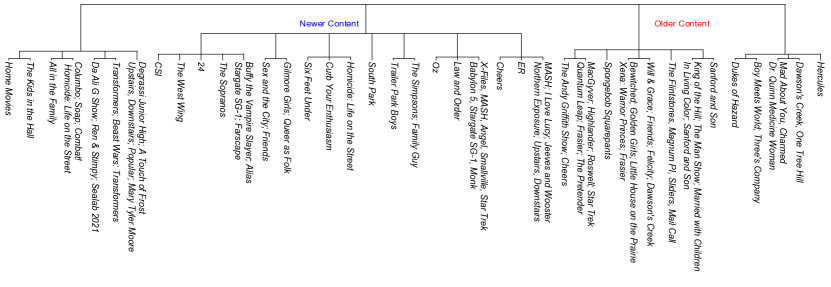
Figure 4: Hierarchy of TV Shows on Netflix based on the first three stencils generated by ACCAMS.

2001: A Space Odyssey	Sex and the City: Season 1	Seinfeld: Seasons 1 & 2	Mean Girls
Taxi Driver	Sex and the City: Season 2	Seinfeld: Season 3	Clueless
Chinatown	Sex and the City: Season 3	Seinfeld: Season 4	13 Going on 30
Citizen Kane	Sex and the City: Season 4	Curb Your Enthusiasm: Season 1	Best in Show
Dr. Strangelove	Sex and the City: Season 5	Curb Your Enthusiasm: Season 2	Particles of Truth
A Clockwork Orange	Sex and the City: Season 6.1	Curb Your Enthusiasm: Season 3	Charlie’s Angels: Full Throttle
THX 1138: Special Edition	Sex and the City: Season 6.2	Arrested Development: Season 1	Amelie
Apocalypse Now Redux	Hercules: Season 3	Newsradio: Seasons 1 and 2	Me Myself I
The Graduate	Will & Grace: Season 1	The Kids in the Hall: Season 1	Bring it On
Blade Runner	Beverly Hills 90210: Pilot	The Simpsons: Treehouse of Horror	Chaos
The Deer Hunter	The O.C.: Season 1	Spin City: Michael J. Fox	Kissing Jessica Stein
Deliverance	Divine Madness	Curb Your Enthusiasm: Season 4	Nine Innings from Ground Zero
Star Wars: Episode V	The Silence of the Lambs	Scooby-Doo Where Are You?	Law & Order: Season 1
Star Wars: Episode IV	The Sixth Sense	The Flintstones: Season 2	Law & Order: Season 3
Star Wars: Episode VI	Alien: Collector’s Edition	Classic Cartoon Favorites: Goofy	Law & Order: SVU (2)
Battlestar Galactica: Season 1	The Exorcist	Transformers: Season 1 (1984)	Law & Order: Criminal Intent (3)
Raiders of the Lost Ark	Schindler’s List	Tom and Jerry: Whiskers Away!	Law & Order: Season 2
Star Wars: Clone Wars: Vol. 1	The Godfather	Boy Meets World: Season 1	MASH: Season 8
Gladiator: Extended Edition	Seven	The Flintstones: Season 3	ER: Season 1
Star Wars Trilogy: Bonus Material	Colors	Scooby-Doo’s Greatest Mysteries	MASH: Season 7
LOTR: The Fellowship of the Ring	The Godfather, Part II	Care Bears: Kingdom of Caring	Rikki-Tikki-Tavi
LOTR: The Two Towers	GoodFellas: Special Edition	Aloha Scooby-Doo!	The X-Files: Season 6
Indiana Jones Trilogy: Bonus Material	Platoon	Scooby-Doo: Legend of the Vampire	The X-Files: Season 7
LOTR: The Return of the King	Full Metal Jacket	Rugrats: Decade in Diapers	ER: Season 3

Figure 5: For a given movie or TV show on Netflix, we can use the cluster assignments to find related content.

In any model the structure of factors makes assumptions about the form of user preferences and decision making. The fact that our model achieves high-quality matrix completion with a smaller parameter space suggests that our modeling assumptions better match how people make decisions. One side effect of our model being both compact and conceptually simple is that we can understand our learned parameters.

To test the model’s interpretability we use ACCAMS to model the Netflix data with $s=20$ stencils and $k^{2}=100$ clusters (a model of similar size to a rank-3 matrix factorization). Here we look at two ways to interpret the results.

First we view the cluster assignments in stencils as inducing a hierarchy on the movies. That is, movies are split in the first level based on their cluster assignments in the first stencil. At the second level, we split movies based on their cluster assignments in the second stencil, etc. In Figure 5 we observe the hierarchy of TV shows induced by the first three stencils learned by ACCAMS (we only include shows where there is more than one season of that show in the leaf and we pruned small partitions due to space restrictions).

As can be seen in the hierarchy, there are branches which clearly cluster together shows more focused on male audiences, female audiences, or children. However, beyond a first brush at the leaf nodes, we can notice some larger structural differences. For example, looking at the two large branches coming from the root, we observe that the left branch generally contains more recent TV shows from the late 1990s to the present, while the right branch generally contains older shows ranging from the 1960s to the mid 1990s. This can be most starkly noticed by “Friends,” which shows up in both branches; Seasons 1 to 4 of “Friends” from 1994-1997 fall in the older branch, while Seasons 5 to 9 from 1998-2002 fall in the newer branch. Of course the algorithm does not know the dates the shows were released, but our model learns these general concepts just based on the ratings. From this it is clear the stencils can be useful for breaking down content in a meaningful structured way, something that is not possible under classic factorization approaches.

While the hierarchy demonstrates that our stencils are learning meaningful latent factors, it may be difficult to always understand individual clusters. Rather, to use knowledge from all of the stencils, we can look to the use case of “Users who watched $X$ also liked $Y$,” and ask given a movie or TV show to search, can we find other similar items? We do this by comparing the set of cluster assignments from the given movie to the set of cluster assignments of other items. We measure similarity between two movies using the Hamming distance between cluster assignments.

As can be seen in Table 5, we find the combination of clusters for different movies and TV shows can be used to easily find similar content. While we see some obvious cases where the method succeeds, e.g. “Sex and the City” returns six more seasons of “Sex and the City,” we also notice the method takes into account more subtle similarities of movies beyond genre. For example, while the first season of “Seinfeld” returns the subsequent seasons of “Seinfeld,” it is followed by three seasons of “Curb Your Enthusiasm,” another comedy show by the same writer Larry David. Similarly, searching for Stanley Kubrick’s “2001: A Space Odyssey” returns other Stanley Kubrick movies, as well as other critically acclaimed films from that era, particularly thematically similar science fiction movies. Searching for “Scooby-Doo” returns topically similar children’s shows, specifically from the mid to late 1900’s. From this we get a sense that ACCAMS does not just find similarity in genre but also more subtle similarities.

Original	Stencil 1	Stencil 2

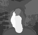
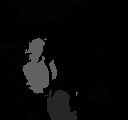
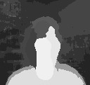
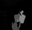
Figure 6: Examples of original images and the first two stencils. The decomposition is very similar to that of eigenfaces [25], albeit much more concise in its nature.

5.6 Properties of ACCAMS

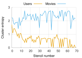
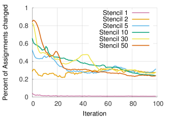
Figure 7: Left: Entropy in cluster assignments for users and movies. Right: Stability of the assignments in the sampler.

Aside from ACCAMS’s success across matrix completion and approximation, it is valuable to understand how our method is working, particularly because of how different it is from previous models. First, because ACCAMS uses backfitting, we expect that the first stencil captures the largest features, the second captures secondary ones, etc. This idea is backed up by our theoretical results in Section 3.3, and we observe that this is working experimentally by the drop off in RMSE for our matrix approximation results in Figure 3. We can visually observe this in the image approximation of the CMU Faces. As can be seen in Figure 6, the first stencil captures general structures of the room and heads, and the second starts to fill in more fine grained details of the face.

The Bayesian model, bACCAMS, backfits in the first iteration of the sampler but ultimately resamples each stencil many times thus loosening these properties. In Figure 7, we observe how the distribution of users and movies across clusters changes over iterations and number of stencils, based on our run of bACCAMS with $s=70$ stencils and a maximum of $k=10$ clusters per stencil. As we see in the plot of entropy, movies, across all 70 stencils, are well distributed across the 10 possible clusters. Users, however, are well distributed in the early stencils but then are only spread across a few clusters in later stencils. In addition, we notice that while the earlier clusters are stable, later stencils are much less stable with a high percentage of cluster assignments changing. Both of these properties follow from the fact that most users rate very few movies. For most users only a few clusters are necessary to capture their observed preferences. Movies, however, typically have more ratings and more latent information to infer. Thus through all 70 stencils we learn useful clusterings, and our prediction accuracy improves through $s=125$ stencils.

6 Discussion

Here we formulated a model of additive co-clustering. We presented both a $k$-means style algorithm, ACCAMS, as well as a generative Bayesian non-parametric model with a collapsed Gibbs sampler, bACCAMS; we obtained theoretical guarantees for matrix approximation through additive co-clustering; and we showed that our method is concise and accurate on a diverse range of datasets, including achieving the best published accuracy on Netflix.

Given the novelty and initial success of the method, we believe that domain-specific variants of ACCAMS, such as for community detection and topic modeling, can and will lead to new models and improved results. In addition, given the modularity of our framework, it is easy to incorporate side information, such as explicit genre and actor data, in modeling rating data that should lead to improved accuracy and interpretability.

Acknowledgements. We would like to thank Christos Faloutsos for his valuable feedback throughout the preparation of this paper. This research was supported by funds from Google, a Facebook Fellowship, a National Science Foundation Graduate Research Fellowship (Grant No. DGE-1252522), and the National Science Foundation under Grant No. CNS-1314632 and IIS-1408924. Any opinions, findings, and conclusions or recommendations expressed in this material are those of the author(s) and do not necessarily reflect the views of the National Science Foundation, or other funding parties.

References

- [1] E. M. Airoldi, D. M. Blei, S. E. Fienberg, and E. P. Xing. Mixed-membership stochastic blockmodels. Journal of Machine Learning Research, 9:1981–2014, 2008.
- [2] A. Banerjee, I. Dhillon, J. Ghosh, S. Merugu, and D. S. Modha. A generalized maximum entropy approach to bregman co-clustering and matrix approximation. In Proceedings of the tenth ACM SIGKDD international conference on Knowledge discovery and data mining, pages 509–514. ACM, 2004.
- [3] A. Beutel, K. Murray, C. Faloutsos, and A. J. Smola. Cobafi: collaborative bayesian filtering. In World Wide Web Conference, pages 97–108, 2014.
- [4] Alex Gittens and Michael W. Mahoney. Revisiting the nyström method for improved large-scale machine learning. In ICML (3), pages 567–575, 2013.
- [5] Y. Gordon, H. König, and C. Schütt. Geometric and probabilistic estimates for entropy and approximation numbers of operators. Journal of Approximation Theory, 49:219–239, 1987.
- [6] D. Görür, F. Jäkel, and C. E. Rasmussen. A choice model with infinitely many latent features. In Proceedings of the 23rd international conference on Machine learning, pages 361–368. ACM, 2006.
- [7] T. Griffiths and Z. Ghahramani. The indian buffet process: An introduction and review. Journal of Machine Learning Research, 12:1185−1224, 2011.
- [8] N. Halko, P.G. Martinsson, and J. A. Tropp. Finding structure with randomness: Stochastic algorithms for constructing approximate matrix decompositions, 2009. oai:arXiv.org:0909.4061.
- [9] J. A. Hartigan. Direct clustering of a data matrix. Journal of the american statistical association, 67(337):123–129, 1972.
- [10] Y. Koren. Factorization meets the neighborhood: a multifaceted collaborative filtering model. In Knowledge discovery and data mining KDD, pages 426–434, 2008.
- [11] Y. Koren, R.M. Bell, and C. Volinsky. Matrix factorization techniques for recommender systems. IEEE Computer, 42(8):30–37, 2009.
- [12] D. Koutra, U. Kang, J. Vreeken, and C. Faloutsos. VOG: Summarizing and Understanding Large Graphs, chapter 11, pages 91–99. SIAM, 2014.
- [13] A. Kyrola, G. Blelloch, and C. Guestrin. Graphchi: Large-scale graph computation on just a pc. In OSDI, Hollywood, CA, 2012.
- [14] J. Lee, S. Kim, G. Lebanon, and Y. Singer. Local low-rank matrix approximation. In Proceedings of The 30th International Conference on Machine Learning, pages 82–90, 2013.
- [15] M. Leeuwen, J. Vreeken, and A. Siebes. Identifying the components. Data Mining and Knowledge Discovery, 19(2):176–193, 2009.
- [16] Mu Li, Gary L. Miller, and Richard Peng. Iterative row sampling. In FOCS 2013, pages 127–136, 2013.
- [17] L. W. Mackey, M. I. Jordan, and A. Talwalkar. Divide-and-conquer matrix factorization. In Advances in Neural Information Processing Systems, pages 1134–1142, 2011.
- [18] R. Neal. Priors for infinite networks. Technical Report CRG-TR-94-1, Dept. of Computer Science, University of Toronto, 1994.
- [19] K. Palla, D. Knowles, and Z. Ghahramani. An infinite latent attribute model for network data. In International Conference on Machine Learning, 2012.
- [20] E. E. Papalexakis, N. D. Sidiropoulos, and R. Bro. From k-means to higher-way co-clustering: multilinear decomposition with sparse latent factors. Signal Processing, IEEE Transactions on, 61(2):493–506, 2013.
- [21] I. Porteous, E. Bart, and M. Welling. Multi-HDP: A non parametric bayesian model for tensor factorization. In D. Fox and C.P. Gomes, editors, Proceedings of the Twenty-Third AAAI Conference on Artificial Intelligence, pages 1487–1490. AAAI Press, 2008.
- [22] J. Rissanen. Modeling by shortest data description. Automatica, 14(5):465–471, 1978.
- [23] H. Shan and A. Banerjee. Bayesian co-clustering. In Data Mining, 2008. ICDM’08. Eighth IEEE International Conference on, pages 530–539. IEEE, 2008.
- [24] A. J. Smola. Learning with Kernels. PhD thesis, Technische Universität Berlin, 1998. GMD Research Series No. 25.
- [25] M. Turk and A. Pentland. Face recognition using eigenfaces. In Proceedings CVPR, pages 586–591, Hawaii, June 1991.
- [26] J. Vreeken, M. Leeuwen, and A. Siebes. Krimp: mining itemsets that compress. Data Mining and Knowledge Discovery, 23(1):169–214, 2011.
- [27] P. Wang, K. B. Laskey, C. Domeniconi, and M. I. Jordan. Nonparametric bayesian co-clustering ensembles. In SDM, pages 331–342. SIAM, 2011.
- [28] L. A. Wolsey. An analysis of the greedy algorithm for the submodular set covering problem. Combinatorica, 2(4):385–393, 1982.