Abstract

It was shown that an infinite sequence of improving non-increasing upper bounds to the ground state energy (GSE) of a slow-moving piezoeletric polaron can be devised.

Key words: piezoelectric polaron, ground state energy, upper bound, variational method

PACS: 71.38.-k, 71.38.Fp

1. The piezoelectric polaron model

A quantized polaron model for the case of an electron interacting with acoustic phonons through piezoelectric deformation potential was introduced by A.R. Hutson [1], its Hamiltonian structure being similar to the Fröhlich optical polaron model introduced by H. Fröhlich [3] earlier:

(1) $$H=\frac{\hat{\bf p}^{2}}{2m}+\displaystyle\sum_{\bf k}\hbar\omega_{{\bf k}}{b^{+}_{\bf k}}{b_{\bf k}}+\displaystyle\sum_{\bf k}\tilde{V}_{k}\left({b^{+}_{\bf k}}e^{-i{\bf k}\hat{\bf r}}+{b_{\bf k}}e^{i{\bf k}\hat{\bf r}}\right),$$

where $\omega_{{\bf k}}=sk$ is the frequency of the acoustical phonons with $s$ being the velocity of sound,

$$\tilde{V}_{k}=\left(\frac{4\pi\alpha}{\tilde{V}}\right)^{1/2}\frac{\hbar^{2}}{m}k^{-1/2},$$

where $\tilde{V}$ is the volume of the crystal, and

$$\alpha=\frac{1}{2}e^{2}\frac{\langle e^{2}_{ijk}\rangle}{\varepsilon Cs\hbar}$$

is the dimensionless coupling constant where $\langle e^{2}_{ijk}\rangle$ is an average of the piezoelectric tensor [1], $\varepsilon$ is the dielectric constant and $C$ is an average elastic constant. The operators $\hat{\bf p}$ and $\hat{\bf r}$ are the electron momentum and position coordinate quantum operators,

$$\quad[\hat{p}_{i},\hat{r}_{j}]=-i\hbar\delta_{ij},$$

and the Bose operators $b^{+}_{{\bf k}}$, $b_{{\bf k}}$,

$$[b_{{\bf k}},b_{{\bf k}^{\prime}}^{+}]=\delta_{{\bf k}{\bf k}^{\prime}},\quad[b_{{\bf k}},b_{{\bf k}^{\prime}}]=0,$$

create and annihilate phonons of one effective acoustic mode of energy $\hbar\omega_{{\bf k}}$ and wave vector ${\bf k}$.

In what follows the energies will be expressed in units of $2ms^{2}$, the length in units of $\hbar/2ms$ and the phonon wave vectors in units of $2ms/\hbar$ so that all variables are dimensionless. In this units the model (1) reads as

(2) $$H=\hat{\bf p}^{2}+\displaystyle\sum_{\bf k}k{b^{+}_{\bf k}}{b_{\bf k}}+\displaystyle\sum_{\bf k}V_{k}\left({b^{+}_{\bf k}}e^{-i{\bf k}\hat{\bf r}}+{b_{\bf k}}e^{i{\bf k}\hat{\bf r}}\right),$$

with

$$V_{k}=\left(\frac{4\pi\alpha}{V}\right)^{1/2}k^{-1/2},$$

where $V$ is dimensionless volume. Ultimately, the sum over the phonon vectors $\sum_{{\bf k}}$ is to be replaced by the integral $V/(2\pi)^{3}\int d{\bf k}$ with a finite cutoff at $k_{0}$, the boundary of the first Brillouin zone in the phonon wave vector space, which is introduced to account for the discreteness of the crystal lattice with $k_{0}\sim 1/a$, where $a$ is the lattice constant.

2. Piezoelectric polaron GSE

As usual, one can introduce the polaron total momentum

$$\hat{\bf P}=\hat{\bf p}+\displaystyle\sum_{{\bf k}}{\bf k}{b^{+}_{\bf k}}{b_{\bf k}}$$

being a constant of the motion and commuting with the Hamiltonian (1). Hence, the Hamiltonian can be transformed to the representation in which $\hat{\bf P}$ becomes a ”c”-number $P$, the value of the total polaron momentum,

$$H\to\tilde{H},\quad\tilde{H}=S^{-1}HS,\quad S=\exp(-i\displaystyle\sum_{{\bf k}}{\bf k}\hat{\bf r}{b^{+}_{\bf k}}{b_{\bf k}}),$$

(3) $$\tilde{H}=({\bf P}-\displaystyle\sum_{{\bf k}}{\bf k}{b^{+}_{\bf k}}{b_{\bf k}})^{2}+\displaystyle\sum_{\bf k}k{b^{+}_{\bf k}}{b_{\bf k}}+\displaystyle\sum_{\bf k}V_{k}\left({b^{+}_{\bf k}}+{b_{\bf k}}\right),$$

and the Hamiltonian (3) does not contain the electron coordinates anymore. One more subsequent transformation

$$\tilde{H}\to{\mathcal{H}}(f),\quad{\mathcal{H}}(f)=U^{-1}\tilde{H}U,\quad U=\exp\{\displaystyle\sum_{{\bf k}}f_{{\bf k}}({b^{+}_{\bf k}}-{b_{\bf k}})\},$$

results in the Hamiltonian

(4) $${\mathcal{H}}(f)={\mathcal{H}}_{0}(f)+{\mathcal{H}}_{1}(f),$$

where

$${\mathcal{H}}_{0}(f)=P^{2}+\displaystyle\sum_{{\bf k}}k{b^{+}_{\bf k}}{b_{\bf k}}+(\displaystyle\sum_{{\bf k}}{\bf k}{b^{+}_{\bf k}}{b_{\bf k}})^{2}-\alpha^{\prime},$$

$${\mathcal{H}}_{1}(f)=\displaystyle\sum_{{\bf k}}[(k+k^{2})f_{{\bf k}}+V_{k}]({b^{+}_{\bf k}}+{b_{\bf k}})+2\displaystyle\sum_{{\bf k}{\bf m}}({\bf k}\cdot{\bf m})f_{{\bf k}}f_{{\bf m}}{b^{+}_{\bf k}}{b_{\bf m}}+$$

$$+\displaystyle\sum_{{\bf k}{\bf m}}({\bf k}\cdot{\bf m})f_{{\bf k}}f_{{\bf m}}({b^{+}_{\bf k}}{b^{+}_{\bf m}}+{b_{\bf k}}{b_{\bf m}})+2\displaystyle\sum_{{\bf k}{\bf m}}({\bf k}\cdot{\bf m})f_{{\bf k}}({b^{+}_{\bf m}}{b_{\bf m}}{b_{\bf k}}+{b^{+}_{\bf k}}{b^{+}_{\bf m}}{b_{\bf m}})-$$

$$-2\displaystyle\sum_{{\bf k}}({\bf P}\cdot{\bf k})({b^{+}_{\bf k}}+f_{{\bf k}})({b_{\bf k}}+f_{{\bf k}})+$$

(5) $$+2\displaystyle\sum_{{\bf k}{\bf m}}({\bf k}\cdot{\bf m})f_{{\bf m}}^{2}{b^{+}_{\bf k}}{b_{\bf k}}+2\displaystyle\sum_{{\bf k}{\bf m}}({\bf k}\cdot{\bf m})f_{{\bf m}}^{2}({b^{+}_{\bf k}}+{b_{\bf k}})+\displaystyle\sum_{{\bf k}{\bf m}}({\bf k}\cdot{\bf m})f_{{\bf m}}^{2}f_{{\bf k}}^{2},$$

and

$$-\alpha^{\prime}=2\displaystyle\sum_{{\bf k}}V_{k}f_{{\bf k}}+\displaystyle\sum_{{\bf k}}(k+k^{2})f^{2}_{{\bf k}}+(\displaystyle\sum_{{\bf k}}f^{2}_{{\bf k}}{\bf k})^{2}.$$

3. On improvable upper bounds to various polaron models GSE in general

Our objective here is to demonstrate that an infinite, in principle, sequence of improvable upper bounds to the ground state energy $E(\alpha,{\bf P},k_{0})$ of the Hamiltonian (4) can be constructed in a regular way by means of a variational method outlined in [4]. Similar variational approach was formulated later in [5]. This energy corresponds to the lowest energy of the slow-moving polaron for a given value of the total polaron momentum ${\bf P}$. Of course, some reservations are to be made here regarding the fact that, unlike in the case of optical polaron, there is no energy separation between the polaron ground state and the excited states with the same total momentum. Therefore, what is considered here is actually a zero temperature polaron behavior.

Then, expansion of the function $E_{g}(\alpha,{\bf P},k_{0})$ in powers of ${\bf P}$ of the kind

$$E_{g}(\alpha,{\bf P},k_{0})=E_{g}(\alpha,0,k_{0})+\frac{P^{2}}{2m_{eff}}+O(P\,^{4}),$$

where $E_{g}(\alpha,0,k_{0})$ is the GSE of the polaron at rest, may provide us with some approximate value of the polaron effective mass $m_{eff}$ in spatially isotropic as well as anisotropic case, in which general case the so-called inverse effective mass tensor $\left(\frac{1}{m_{eff}}\right)_{ij}$ is to be introduced as

$$\left(\frac{1}{m_{eff}}\right)_{ij}=\frac{\partial^{2}E(\alpha,{\bf P},k_{0})}{\partial P_{i}\partial P_{j}}\Bigg{|}_{{\bf P}=0}.$$

instead of the scalar effective mass parameter $m_{eff}$.

As was shown in [4], for a quantum system Hamiltonian $\hat{H}$ and a trial state $|\psi\rangle$,  such that $\langle\psi|\psi\rangle=1$,

$$E_{g}\leq\min(a_{1}^{(n)},...,a_{n}^{(n)})\leq\langle\psi|\hat{H}|\psi\rangle,$$

where the real numbers $(a_{1}^{(n)},...,a_{n}^{(n)})$ are the roots of the n-th order polynomial equation

$$P_{n}(x)=\displaystyle\sum_{i=0}^{n}X_{i}x^{n-i}=0.$$

Here, the coefficient $X_{0}\equiv 1$ and all the other coefficients $X_{i}$,  $1\leq i\leq n$ satisfy the system of $n$ linear equations

$${\mathcal{M}}{\bf X}+{\bf Y}=0,$$

with

$$Y_{i}=M_{2n-i},\quad{\mathcal{M}}_{ij}=M_{2n-(i+j)},\quad i,j=1,2,...n,$$

and

$$M_{m}=\langle\psi|\hat{H}^{m}|\psi\rangle.$$

It is assumed that all moments $M_{m}$ are finite. It was proved that the following inequality holds

$$\min(a_{1}^{(n+1)},...,a_{n+1}^{(n+1)})\leq\min(a_{1}^{(n)},...,a_{n}^{(n)}).$$

So, at the first order

(6) $$E_{g}\leq a_{1}^{(1)},\qquad a_{1}^{(1)}=\langle\psi|\hat{H}|\psi\rangle,$$

and at the second order

(7) $$E_{g}\leq\min(a_{1}^{(2)},a_{2}^{(2)})=\langle\psi|\hat{H}|\psi\rangle+\frac{K_{3}}{2K_{2}}-\left[\left(\frac{K_{3}}{2K_{2}}\right)^{2}+K_{2}\right]^{1/2},$$

$$a_{1}^{(2)}=\langle\psi|\hat{H}|\psi\rangle+\frac{K_{3}}{2K_{2}}-\left[\left(\frac{K_{3}}{2K_{2}}\right)^{2}+K_{2}\right]^{1/2},$$

$$a_{2}^{(2)}=\langle\psi|\hat{H}|\psi\rangle+\frac{K_{3}}{2K_{2}}+\left[\left(\frac{K_{3}}{2K_{2}}\right)^{2}+K_{2}\right]^{1/2},$$

where $K_{2}$ and $K_{3}$ are the central moments

$$K_{2}=\langle\psi|(\hat{H}-\langle\psi|\hat{H}|\psi\rangle)^{2}|\psi\rangle,\qquad K_{3}=\langle\psi|(\hat{H}-\langle\psi|\hat{H}|\psi\rangle)^{3}|\psi\rangle.$$

It is seen that the second order bound (7) would lie below the first order bound (6) for most physically relevant quantum models and most reasonable and meaningful choices of the trial state $|\psi\rangle$.

4. Improvable upper bounds for piezoelectric polaron at rest

For ${\bf P}=0$, the function $f_{{\bf k}}$ is spherically symmetric, and the piezoelectric polaron modelHamiltonian (4) reduces to

$${\mathcal{H}}(f)=\displaystyle\sum_{{\bf k}}k{b^{+}_{\bf k}}{b_{\bf k}}+(\displaystyle\sum_{{\bf k}}{\bf k}{b^{+}_{\bf k}}{b_{\bf k}})^{2}-\alpha^{\prime}+$$

$$+\displaystyle\sum_{{\bf k}}[(k+k^{2})f_{k}+V_{k}]({b^{+}_{\bf k}}+{b_{\bf k}})+2\displaystyle\sum_{{\bf k}{\bf m}}({\bf k}\cdot{\bf m})f_{k}f_{m}{b^{+}_{\bf k}}{b_{\bf m}}+$$

$$+\displaystyle\sum_{{\bf k}{\bf m}}({\bf k}\cdot{\bf m})f_{k}f_{m}({b^{+}_{\bf k}}{b^{+}_{\bf m}}+{b_{\bf k}}{b_{\bf m}})+2\displaystyle\sum_{{\bf k}{\bf m}}({\bf k}\cdot{\bf m})f_{k}({b^{+}_{\bf m}}{b_{\bf m}}{b_{\bf k}}+{b^{+}_{\bf k}}{b^{+}_{\bf m}}{b_{\bf m}}).$$

As to be seen later on, it would be convenient to choose phonon vacuum state $|0\rangle$ as a trial state $|\psi\rangle$ for ${\mathcal{H}}(f)$,  so that inequality

$$E_{g}(\alpha,0,k_{0})\leq\langle 0|{\mathcal{H}}(f)|0\rangle=2\displaystyle\sum_{{\bf k}}V_{k}f_{k}+\displaystyle\sum_{{\bf k}}(k+k^{2})f^{2}_{k}$$

holds, the right-hand side of which is minimized by

$$f_{k}=-V_{k}/(k+k^{2}),$$

and, eventually,

(8) $$E_{g}(\alpha,0,k_{0})\leq E_{W}(\alpha,0,k_{0})=-\frac{2\alpha}{\pi}\ln[1+k_{0}].$$

The upper bound (8) stems from the conventional variational principle in quantum mechanics and is valid for arbitrary value of $\alpha$. To derive a sequence of better non-increasing upper bounds one needs to calculate moments $\langle 0|{\mathcal{H}}^{m}(f)|0\rangle$ for sufficiently large integer exponents $m$ by means of the Wick theorem. The result of the calculation for any such moment can be expressed in terms of the products of integrals of rational functions

(9) $$\int_{0}^{k_{0}}\frac{k^{p}dk}{(k+k^{2})^{q}},\qquad p,q-\mbox{non-negative integers},$$

which can be evaluated analytically.

Thus, at the second order variational approximation (7)

(10) $$E_{g}(\alpha,0,k_{0})\leq E_{var}=-\frac{2\alpha}{\pi}\ln[1+k_{0}]+\frac{K_{3}}{2K_{2}}-\left[\left(\frac{K_{3}}{2K_{2}}\right)^{2}+K_{2}\right]^{1/2},$$

where

(11) $$K_{2}=\frac{8\alpha^{2}}{3\pi^{2}}F_{1}^{2}(k_{0}),$$

(12) $$K_{3}=\frac{16\alpha^{2}}{3\pi^{2}}(F_{1}(k_{0})F_{2}(k_{0})+F_{1}(k_{0})F_{3}(k_{0}))+\frac{64\alpha^{3}}{9\pi^{3}}F_{1}^{3}(k_{0}),$$

(13) $$F_{1}(k_{0})=\left[\ln(1+k_{0})+\frac{1}{1+k_{0}}-1\right],$$

(14) $$F_{2}(k_{0})=\left[\frac{k_{0}^{2}}{2}-k_{0}+\ln(1+k_{0})\right],$$

(15) $$F_{3}(k_{0})=\left[-2k_{0}+\frac{k_{0}^{2}}{2}+3\ln(1+k_{0})+\frac{1}{1+k_{0}}-1\right]$$

This upper bound is worth comparing with the lower bounds to the piezoelectric polaron GSE obtained in [6] for the case of small

(16) $$E_{LBS}\approx-(2\alpha/\pi)\ln(k_{0}+1),\qquad\alpha\ll 1,$$

and large

(17) $$E_{LBL}\approx-\frac{1}{3}\alpha^{2}-(4\alpha/\pi)\ln(k_{0}/\alpha),\qquad 1\ll\alpha\ll k_{0}$$

coupling constant respectively. The bound $E_{LBS}$ coincides, actually, with the perturbation theory result [7]. It was assumed in [6] that $k_{0}\approx 150$. So, the bounds (8), (16) and (17) are plotted in Figs.1-3 just for this value of $k_{0}$.

5. Improvable upper bounds to the GSE of the slow-moving piezoelectric polaron

In general case ${\bf P}\neq 0$

$$E_{g}(\alpha,{\bf P},k_{0})\leq\langle 0|{\mathcal{H}}(f)|0\rangle=P^{2}+2\displaystyle\sum_{{\bf k}}V_{k}f_{{\bf k}}+\displaystyle\sum_{{\bf k}}(k+k^{2})f^{2}_{{\bf k}}-2\displaystyle\sum_{{\bf k}}({\bf P}\cdot{\bf k})f^{2}_{{\bf k}}+(\displaystyle\sum_{{\bf k}}f^{2}_{{\bf k}}{\bf k})^{2},$$

with the right-hand side to be minimized by

$$f_{{\bf k}}=-V_{k}/[k-2{\bf k}\cdot{\bf P}(1-\eta)+k^{2}],$$

where $\eta$ is defined self-consistently by the equation

$$\eta{\bf P}=\displaystyle\sum_{{\bf k}}f^{2}_{{\bf k}}{\bf k}=\displaystyle\sum_{{\bf k}}V_{k}^{2}{\bf k}/[k-2{\bf k}\cdot{\bf P}(1-\eta)+k^{2}]^{2},$$

or, alternatively, by

$$\eta P^{2}=\displaystyle\sum_{{\bf k}}V_{k}^{2}{\bf k}\cdot{\bf P}/[k-2{\bf k}\cdot{\bf P}(1-\eta)+k^{2}]^{2}.$$

The resulting upper bound is

(18) $$E_{g}(\alpha,{\bf P},k_{0})\leq P^{2}(1-\eta)^{2}-\displaystyle\sum_{{\bf k}}V_{k}^{2}\frac{k+k^{2}-4{\bf k}\cdot{\bf P}(1-\eta)}{[k-2{\bf k}\cdot{\bf P}(1-\eta)+k^{2}]^{2}}.$$

Another choice

(19) $$f_{{\bf k}}=-[V_{k}+2\eta{\bf k}\cdot{\bf P}]/[k-2{\bf k}\cdot{\bf P}+k^{2}],$$

eliminating all terms linear in Bose operators ${b^{+}_{\bf k}}$, ${b_{\bf k}}$ in (4), is possible too, with the corresponding self-consistency equation for $\eta$

$$\eta P^{2}=\displaystyle\sum_{{\bf k}}f^{2}_{{\bf k}}{\bf k}=\displaystyle\sum_{{\bf k}}{\bf k}\cdot{\bf P}[V_{k}+2\eta{\bf k}\cdot{\bf P}]^{2}/[k-2{\bf k}\cdot{\bf P}+k^{2}]^{2},$$

which can be solved analytically. At the same time, the simplest choice

$$f_{k}=-V_{k}/(k+k^{2})$$

seems to be preferable, because in this case the complexity of the analytical calculation of arbitrary moments $\langle 0|{\mathcal{H}}^{m}(f)|0\rangle$ does not exceed the one for the case ${\bf P}=0$, i.e. no employment of any integrations over wave vectors more complicated and laborious than the integrals of the type (9) is necessary.

6. Summary

It was shown that the GSE function $E_{g}(\alpha,{\bf P},k_{0})$ of the slow-moving piezoelectric polaron can be approximated by infinite sequence of non-increasing upper bounds for arbitrary values of the coupling constant $\alpha$, polaron total momentum ${\bf P}$ and cut-off wave vector $k_{0}$. The proposed algorithm for the construction of these bounds is well-suited for implementation by means of contemporary techniques for parallel computing due to its overwhelming reliance on the Wick theorem.

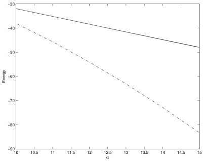
Figure 1. Upper bounds: $E_{var}$, solid line; $E_{LBS}$, dashed line; $E_{LBL}$, dash-dotted line; $k_{0}=150$.

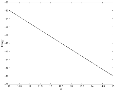
Figure 2. Upper bounds: $E_{var}$, solid line; $E_{LBS}$, dashed line; $k_{0}=150$.

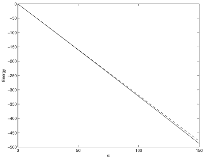
Figure 3. Upper bounds: $E_{var}$, solid line; $E_{LBS}$, dashed line; $k_{0}=150$.

References

• [1] HutsonΒ A.R., J. Appl. Phys., 1961, 32, 2287.
• [2] FrΓΆhlichΒ H., Proc. Roy. Soc. A, 1937, 160, 230.
• [3] FrΓΆhlichΒ H., Advan. Phys., 1954, 3, 325.
• [4] SoldatovΒ A.V., Int. J. Mod. Phys. B, 1995, 9, n.22, 2899.
• [5] KireevΒ A.N., Int. J. Mod. Phys. B, 1997, 11, n.10, 1235.
• [6] ThomchickΒ J., WhitfieldΒ G., Phys. Rev. B, 1974, 9, 1506.
• [7] ThomchickΒ J., WhitfieldΒ G., GerstnerΒ J., TharmalingamΒ K., Phys. Rev., 1968, 165, 993.
Refer to caption