Galaxy Cluster Pressure Profiles as Determined by Sunyaev Zel’dovich Effect Observations with MUSTANG and Bolocam I: Joint Analysis Technique

Abstract

We present a technique to constrain galaxy cluster pressure profiles by jointly fitting Sunyaev-Zel’dovich effect (SZE) data obtained with MUSTANG and Bolocam for the clusters Abell 1835 and MACS0647. Bolocam and MUSTANG probe different angular scales and are thus highly complementary. We find that the addition of the high resolution MUSTANG data can improve constraints on pressure profile parameters relative to those derived solely from Bolocam. In Abell 1835 and MACS0647, we find gNFW inner slopes of $\gamma=0.36_{-0.21}^{+0.33}$ and $\gamma=0.38_{-0.25}^{+0.20}$, respectively when $\alpha$ and $\beta$ are constrained to $0.86$ and $4.67$ respectively. The fitted SZE pressure profiles are in good agreement with X-ray derived pressure profiles.

1. Introduction

Galaxy clusters are the largest gravitationally bound objects in the universe and thus serve as ideal cosmological probes and astrophysical laboratories. Because the formation of galaxy clusters stems from overdensities of matter and depends on the cosmic composition of the universe, one can constrain cosmological parameters such as the matter density of the universe, $\Omega_{m}$, the matter power spectrum normalization, $\sigma_{8}$, and the equation of state for dark energy density $\Omega_{\Lambda}$, $w$ (e.g. Carlstrom et al., 2002).

Within a galaxy cluster, the gas in the intracluster medium (ICM) constitutes 90% of the baryonic mass (Vikhlinin et al., 2006) and is directly observable in the X-ray due to bremsstrahlung emission. At millimeter and sub-millimeter wavelengths, the ICM is observable via the Sunyaev-Zel’dovich effect (SZE) (Sunyaev & Zel’dovich, 1972): the inverse Compton scattering of cosmic microwave background (CMB) photons off of the hot ICM electrons. The thermal SZE is observed as an intensity decrement relative to the CMB at wavelengths longer than $\sim$1.4 mm (frequencies less than $\sim$220 GHz). At longer radio wavelengths, if relativistic electrons are present, parts of the ICM may emit synchrotron emission.

In the core of a galaxy cluster, baryonic physics are non-negligible and non-trivial. Some observed physical processes in the core include shocks and cold fronts (e.g. Markevitch & Vikhlinin, 2007), sloshing (e.g. Fabian et al., 2006), and X-ray cavities (McNamara & Nulsen, 2007). It is also theorized that helium sedimentation should occur, most noticeably in low redshift, dynamically-relaxed clusters (Abramopoulos et al., 1981; Gilfanov & Syunyaev, 1984) and recently the expected helium enhancement via sedimentation has been numerically simulated (Peng & Nagai, 2009). This would result in an offset between X-ray and SZE derived pressure profiles.

At large radii ($R\gtrsim R_{500}$), equilibration timescales are longer, accretion is ongoing, and hydrostatic equilibrium (HSE) is a poor approximation. Several numerical simulations show that the fractional contribution from non-thermal pressure increases with radius (Shaw et al., 2010; Battaglia et al., 2012; Nelson et al., 2014). For all three studies, non thermal pressure fractions between 15% and 30% are found at ($R\sim R_{500}$) for redshifts $0<z<1$. However, the intermediate radii, between the core and outer regions of the galaxy cluster, offer a region where self-similar scalings derived from HSE can be used to describe simulations and observations (e.g. Kravtsov & Borgani, 2012). Moreover, both simulations and observations find low cluster-to-cluster scatter in pressure profiles within this intermediate radial range (e.g. Borgani et al., 2004; Nagai et al., 2007; Arnaud et al., 2010; Bonamente et al., 2012; Planck Collaboration et al., 2013; Sayers et al., 2013).

While many telescopes capable of making SZE observations are already operational or are being built, most have angular resolutions (full width, half maximum - FWHM) of one arcminute or larger. The MUSTANG instrument (Dicker et al., 2008) on the 100 meter Robert C. Byrd Green Bank Telescope (GBT, Jewell & Prestage, 2004) with its angular resolution of $9\mbox{${}^{\prime\prime}$}$ (FWHM) and sensitivity up to the limit of MUSTANG’s instantaneous field of view, $1$^′, is one of only a few SZE instruments with sub-arcminute resolution. To probe a wider range of scales we complement our MUSTANG data with SZE data from Bolocam (Glenn et al., 1998). Bolocam is a 144-element bolometer array on the Caltech Submillimeter Observatory (CSO) with a beam FWHM of $58\mbox{${}^{\prime\prime}$}$ at 140 GHz and circular FOV with $8^{\prime}$ diameter, which is well matched to the angular size of $R_{500}$ ($\sim 4$^′) for both of the clusters in our sample.

In this paper, we extend the map fitting technique used in Young et al. (2014), to simultaneously fit 3D pressure profiles to Bolocam and MUSTANG data. With MUSTANG’s high resolution, this is the first analysis to make use of SZE observations that cover similar scales ($0.03R_{500}<r\lesssim R_{500}$) to those probed by X-ray studies (Nagai et al., 2007; Arnaud et al., 2010, ; hereafter N07 and A10 respectively) which have constrained the average cluster pressure profile. N07 compared X-ray and simulation results over radial scales ($0.1R_{500}\lesssim r\lesssim R_{500}$), whereas A10 used X-ray determined pressure profiles for $0.03R_{500}\lesssim r<R_{500}$, and simulation results for $R_{500}<r$. More recently, the Planck collaboration has published an analysis combining XMM-Newton observations, which span ranges $0.02R_{500}<r<R_{500}$ with Planck observations, which span radial ranges $0.1R_{500}<r<3R_{500}$ (Planck Collaboration et al., 2013). Additionally, a sample of clusters studied by Bolocam has been analyzed using solely the SZE data, which spans radial ranges of $0.07R_{500}<r<3.5R_{500}$ (Sayers et al., 2013).

This paper is organized as follows. In Section 2 we describe the MUSTANG and Bolocam observations and reduction. In Section 3 we detail the method used to jointly fit pressure profiles to MUSTANG and Bolocam data. We present results from the joint fits in Section 4 and discuss our results in Section 5. Throughout this paper we assume a flat $\Lambda$CDM cosmology with $\Omega_{m}=0.3$, $\Omega_{\lambda}=0.7$, and $H_{0}=70$ km s^-1 Mpc^-1, consistent with the 9-year Wilkinson Microwave Anisotropy Probe (WMAP) results reported in Hinshaw et al. (2013).

2. Observations and Data Reduction

2.1. Sample

To test the application of the joint fitting technique, we use two clusters: MACS J0647.4+7015 and Abell 1835. Properties of these two clusters are shown in Table 2.1. MACS 0647 (Ebeling et al., 2007, 2010) has been observed by MUSTANG as part of an SZE program to observe the Cluster Lensing and Supernova with Hubble (CLASH) sample (Postman et al., 2012). MACS J0647 is well detected by MUSTANG and appears to be relaxed; thus it presents a good baseline for testing our fitting procedure. We note that it has been previously analyzed (Young et al., 2014), albeit with a slightly different approach. Abell 1835 is a well known cool core cluster (e.g. Peterson et al., 2001), with prior SZE detections (e.g. Reese et al., 2002; Benson et al., 2004; Bonamente et al., 2006; Sayers et al., 2011; Mauskopf et al., 2012). MUSTANG detects the cluster along with a point source in the center of the cluster, thus making it a good cluster to demonstrate that the joint fitting technique established here can distinguish between point source signal and SZE signal.

Table 1Cluster Properties

Cluster	$z$	$R_{500}$	$R_{500}$	$M_{500}$
		(Mpc)	(′)	($10^{14}~{}M_{\odot}$)
A1835	0.253	$1.49\pm 0.06$	$6.30$	$12.3\pm 1.4$
MACS J0647.7	0.591	$1.26\pm 0.06$	$3.16$	$10.9\pm 1.6$

References. — Mantz et al. (2010)

2.2. MUSTANG Observations

MUSTANG is a 64 pixel array of Transition Edge Sensor (TES) bolometers arranged in an $8\times 8$ array located at the Gregorian focus on the 100 m GBT. Operating at 90 GHz (81–99 GHz), MUSTANG has an angular resolution of $9\mbox{${}^{\prime\prime}$}$ and pixel spacing of 0.63$f\lambda$ resulting in a FOV of $42\mbox{${}^{\prime\prime}$}$. More detailed information about the instrument can be found in Dicker et al. (2008).

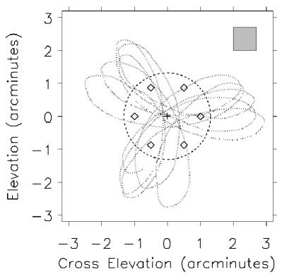
Figure 1.— Dotted line: an example GBT trajectory for a 140 second scan with a Lissajous daisy scan pattern. Three 140 second scans result in complete coverage of a circle with $3^{\prime}$ radius. The plus sign indicates the pointing center used for this daisy scan. The diamonds indicate six offset pointings, used on observations of MACS 0647. The FOV of MUSTANG is shown by the shaded box. The dashed circle encloses 50% of the peak weight over the ensemble of scans for a given cluster.

Observations consisted of scanning on pointing centers covering the central region of each galaxy cluster. A variety of scan durations ranging between 90 and 300 seconds were employed. Over the seasons of observations, we found that scans lasting 200 to 220 seconds provided the best yields, and accordingly we began to favor scans of this length. Abell 1835 was observed in the winter/spring of 2009 and 2010 with one central pointing as described in Korngut et al. (2011). For MACS 0647 (observed 2011-2013), we adopted an observing strategy that consisted of one central pointing, and six off-center pointings, spaced hexagonally such that each was $1\arcmin$ from the center, and $1\arcmin$ away from the other two pointings (Figure 1). Using the offset pointings with a Lissajous daisy scan pattern provides more uniform coverage within the central arcminute of our maps than using only one central pointing with Lissajous daisy scans. For each pointing center, the Lissajous daisy has a $3\arcmin$ radius. The coverage (weight) drops to 50% of its peak value at a radius of $1.3^{\prime}$.

Absolute flux calibrations are based on the planets Mars, Uranus, or Saturn, nebulae, or the star Betelgeuse ($\alpha_{Ori}$). At least one of these flux calibrators was observed at least once per night. Planets and nebulae are the preferred targets, as they can be calibrated directly to WMAP observations (Weiland et al., 2011). Betelgeuse can then be cross calibrated to these planets and nebulae, and may be used as an absolute calibration itself when no planets or nebulae were observed in a given night. We find our calibration is accurate to a 10% RMS uncertainty.

At the start of each night of observing, medium-scale, mostly thermal imperfections in the GBT surface are measured and corrected using out-of-focus (OOF) holographic technique (Nikolic et al., 2007). Interspersed with scans on clusters, we observe nearby compact quasars as secondary calibrators. Secondary calibrators are observed roughly once every 30 minutes, and allow us to track the pointing, beam profile, and gain changes of the telescope. If the the beam shape or gain degrade by more than 10%, another OOF measurement was performed. We find that our pointing accuracy is $2\mbox{${}^{\prime\prime}$}$. We pair the scans on secondary calibrators with off-source scans of an internal calibration lamp (CAL) chopped with a 0.5 Hz square wave pattern. These CAL scans are taken with the telescope at rest.

All observations of calibrators (primary and secondary) also make use of a Lissajous daisy scan pattern. These scans have a duration of 90 seconds and radius of $1.5\arcmin$. This scan pattern ensures that each detector passes over the point source (within the primary beam) multiple times in a scan. Additionally, a radius of $1.5\arcmin$ ensures adequate sampling of the error beam.

Table 2 shows the time spent (on source) observing each cluster. MACS 0647, which had exceptionally good quality data compared to the other cluster, fares better than the expected $t^{-1/2}$ scaling relative to Abell 1835. In Table 2 the noise is calculated from a noise map, produced as described in Section 2.4. Specifically, we smooth the map by convolving it with a Gaussian with FWHM of $10\mbox{${}^{\prime\prime}$}$ and then select the central arcminute ($r<1\arcmin$), where the weight is nearly uniform, and calculate the root-mean-square (RMS) of the selected pixels.

Table 2Dataset Properties for MUSTANG observations

Cluster	Time	Secondary	Noise
	(hrs)	Calibrator	($\mu$Jy/beam)
A1835	8.6	1337-1257	53.3
MACS J0647.7	16.4	0721+7120	20.8

2.3. MUSTANG Beam

The MUSTANG beam is characterized by making calibrated maps of compact sources. Point source maps of bright secondary calibrators, which are in a high signal-to-noise regime, are produced with gentler filtering than is used to create galaxy cluster maps(see Section 2.4); the primary difference is that no common mode is subtracted and we use data from outside the central arcminute to calculate and subtract our polynomial fit. For a single map, the point source centroid is determined by fitting a two dimensional Gaussian to the map using a Levenberg-Marquardt least squares minimization in IDL (MPFIT, Markwardt, 2009). With the centroid determined, pixel values and weights are stored as a function of radius, and the values are normalized based on the peak of the fitted 2D Gaussian. This constitutes the normalized point source profile, or MUSTANG beam profile, for one map. 2D Gaussians are fit to all 185 secondary calibration observations from fall 2011 until spring 2013 with fair quality data: wind speeds below 5 m/s, and FWHM $<11\mbox{${}^{\prime\prime}$}$. The FWHM is taken as the geometric mean of the FWHM along the two axes as fit for below.

To characterize the typical beam for MUSTANG, we assume a one dimensional, double Gaussian:

$$B(r)=B_{1}e^{-\frac{r^{2}}{2\sigma_{1}^{2}}}+B_{2}e^{-\frac{r^{2}}{2\sigma_{2}^{2}}}$$ (1)

where $B_{1}$ is the normalization of the primary beam, and $B_{2}$ is the normalization of the secondary (error) beam. This model is then fit, using MPFIT, to the normalized, azimuthal profiles of all the secondary calibrators to obtain $B_{1}=0.94_{-0.02}^{+0.02}$, $\sigma_{1}=3.69_{-0.14}^{+0.23}$^′′, $B_{2}=0.06_{-0.02}^{+0.02}$, $\sigma_{2}=12.1_{-2.8}^{+3.3}\mbox{${}^{\prime\prime}$}$. This corresponds to a primary beam with FWHM of $8.7\mbox{${}^{\prime\prime}$}$ and a secondary (error) beam with FWHM of $28.4\mbox{${}^{\prime\prime}$}$. Figure 2 shows the fitted beam and normalized pixel values. The secondary beam is qualitatively consistent with the expected near-sidelobes on the GBT given the MUSTANG illumination pattern and medium-scale aperture phase errors not fully corrected by the OOF procedure in Section 2.2.

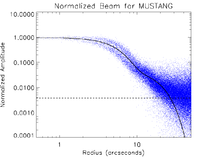
Figure 2.— The solid line shows the fitted radial beam profile of MUSTANG. Fitting a double Gaussian, the primary beam has a FWHM of $8.7\mbox{${}^{\prime\prime}$}$, with normalization, $B_{1}$, of $0.94$. The secondary beam has a FWHM of $28.4\mbox{${}^{\prime\prime}$}$ with a normalization $B_{2}$, of $0.06$. The dashed line shows the weighted RMS of normalized pixels beyond $27\mbox{${}^{\prime\prime}$}$; it intersects the fitted line at $27\mbox{${}^{\prime\prime}$}$.

Given the dispersion in pixel values in Figure 2, we investigate the stability and uncertainty in the fitted parameters. To investigate the stability of the fitted MUSTANG beam, we divide the sample by observing season (fall to spring). Fitting a one dimensional, double Gaussian to the beam profile over five seasons of data, we find minimal variation and consistent dispersion in pixel values. Moreover, the apparent bimodality in the inner beam is present in all seasons, and appears to be due the ellipticity of individual beams. From the original two-dimensional (single Gaussian) fits, we find the mode and median of major-to-minor axis ratios are 1.05 and 1.08 respectively. Taking azimuthal profiles of the fitted (model) two-dimensional Gaussians reveals the same bimodality.

2.4. MUSTANG Reduction

Processing of MUSTANG data is performed using a custom IDL pipeline. Raw data is recorded as time ordered data (TOD) from each of the 64 detectors. An outline of the data processing for each scan on a galaxy cluster is given below.

(1) We define a pixel mask from the nearest preceding CAL scan; unresponsive detectors are masked out. The CAL scan provides us with unique gains to be applied to each of the responsive detectors.

(2) A common mode template is calculated as the arithmetic mean of the TOD across detectors. The pulse tube used to cool the array produces a coherent 1.411 Hz signal across all detectors. A sinusoid is used as a template to fit this signal. The common mode template, pulse tube template, and a polynomial of order $N$ are then simultaneously fit to each detector and then subtracted. The polynomial order is given by $N=t_{scan}/t_{poly}$, where $t_{scan}$ is the scan duration, $t_{poly}=2$^′$/\bar{v}$, and $\bar{v}$ is the mean scan speed. Typically, $t_{poly}$ is roughly $1.0$ seconds, while scan durations vary between $90$ and $180$ seconds. Subtracting the common mode is powerful at removing atmospheric emission, but has the downside of removing astronomical signals much larger than the instrument FOV. For Abell 1835 ($z=0.25$), $42\mbox{${}^{\prime\prime}$}$ corresponds to 166 kpc; for MACS 0647 ($z=0.59$), $42\mbox{${}^{\prime\prime}$}$ corresponds to 285 kpc.

(3) After the common mode and polynomial subtraction, each scan undergoes further data quality checks: spike (glitch) rejection, skewness, and Allan variance. Spikes are flagged such that the remaining TOD is still used, while detectors that fail skewness and Allan variance checks are masked for that scan. In total, MACS 0647 has 11% of its data flagged, and Abell 1835 has 36% of its data flagged.

(4) Individual detector weights are calculated as $1/\sigma_{i}^{2}$, where $\sigma_{i}$ is the RMS of the non-flagged TOD for that detector.

(5) Maps are produced by gridding the TOD in $1\mbox{${}^{\prime\prime}$}$ pixels in Right Ascension (R.A.) and Declination (Dec). A weight map is produced in addition to the signal map. Unsmoothed signal-to-noise (SNR) maps are produced by dividing the signal map by the inverse square root of the weight map. For smoothed SNR maps, the signal and variance maps are smoothed, and the SNR map is then calculated as the signal map divided by the square root of the variance map.

2.5. MUSTANG Noise

Because we are in the small signal limit, we need to understand our noise very well in both the time domain and map (spatial) domain. In the map domain, we can produce noise maps by sending our TOD through the above reduction process and either flipping, i.e. reversing, the TOD per scan in the time domain, or by flipping sign of the gain between scans. The former works by no longer allowing the signal to be coherently matched to location on the sky, while the latter works by effectively cancelling any signal observed. Thorough analysis has shown better behavior in the gain-flipped maps. For instance, if we make an unsmoothed SNR map from the gain-flipped TOD, we find a mean of 0 with a standard deviation of 1. In both the gain- and time-flipped noise maps, we find that pixel weights accurately reflect the RMS of pixel values within a weight bin, and the pixel values follow a Gaussian distribution. Smoothed SNR maps produced from either of the flipped TOD methods produce standard deviations greater than 1; the advantage of the gain-flipped smoothed SNR maps is that their means are 0, whereas the time-flipped SNR maps have means that are offset from 0. The standard deviation of our smoothed noise SNR maps ($\sigma_{SNR}$) tending towards values greater than 1 indicates our smoothing procedure does not accurately handle the weights of each pixel; thus, we use $\sigma_{SNR}$ to correct our true (not noise) SNR maps. For our canonical smoothing kernel ($10\mbox{${}^{\prime\prime}$}$ FWHM), $\sigma_{SNR}\sim 1.6$; we then divide the true SNR map by this factor. As the model fitting presented in this work makes use of only the non-smoothed maps, this correction factor is only used for visualizing smoothed SNR maps.

2.6. Bolocam Observations and Reduction

Bolocam is a 144-element camera that was a facility instrument on the Caltech Submillimeter Observatory (CSO) from 2003 until 2012. Its field of view is $8^{\prime}$ in diameter, and at 140 GHz it has a resolution of $58\mbox{${}^{\prime\prime}$}$ FWHM (Glenn et al. (1998); Haig et al. (2004)). The clusters were observed with a Lissajous pattern that results in a tapered coverage dropping to 50% of the peak value at a radius of roughly $5^{\prime}$, and to 0 at a radius of $10^{\prime}$. The Bolocam maps used in this analysis are $14\arcmin\times 14\arcmin$.

The Bolocam data are the same as those used in Czakon et al. (2014) and Sayers et al. (2013); the details of the reduction are given therein, along with Sayers et al. (2011). Bolocam observed Abell 1835 for 14.0 hours resulting in a noise of 16.2 $\mu K_{CMB}$-arcminute, and observed MACS 0647 for 11.4 hours resulting in a noise of 22.0 $\mu K_{CMB}$-arcminute. Overall, the reduction and calibration is quite similar to that used for MUSTANG, and Bolocam achieves a 5% calibration accuracy and $5\mbox{${}^{\prime\prime}$}$ pointing accuracy.

3. Joint Map Fitting Technique

3.1. Producing Cluster Model Maps

We choose to construct 3D electron pressure profiles as parameterized by a generalized Navarro, Frenk, and White profile (hereafter, gNFW Navarro et al., 1997; Nagai et al., 2007):

$$\tilde{P}=\frac{P_{0}}{(C_{500}X)^{\gamma}[1+(C_{500}X)^{\alpha}]^{(\beta-\gamma)/\alpha}}$$ (2)

where $X=R/R_{500}$, and $C_{500}$ is the concentration parameter; one can also write ($C_{500}X$) as ($R/R_{s}$), where $R_{s}=R_{500}/C_{500}$. $\tilde{P}$ is the electron pressure in units of the characteristic pressure $P_{500}$. The 3D pressure profile is assumed to be spherical and is integrated along the line of sight to produce a Compton $y$ profile, given as

$$y(r)=\frac{P_{500}\sigma_{T}}{m_{e}c^{2}}\int_{-\infty}^{\infty}\tilde{P}(r,l)dl$$ (3)

where $R^{2}=r^{2}+l^{2}$, $r$ is the projected radius, and $l$ is the distance from the center of the cluster along the line of sight. Once integrated, $y(r)$ is gridded as $y(\theta)$ and is realized as a map (pixels of $1\mbox{${}^{\prime\prime}$}$ and $20^{\prime}$ on a side) using the Archive of Chandra Cluster Entropy Profile Tables (ACCEPT, Cavagnolo et al. (2009)) centroid for the cluster. From here, we produce two model maps: one for Bolocam and one for MUSTANG. In each case, we convolve the Compton $y$ map by the appropriate beam shape. For Bolocam we use a Gaussian with FWHM $=58\mbox{${}^{\prime\prime}$}$, and for MUSTANG we use the double Gaussian as found in Section 2.3.

The convolved maps are then regridded to the same scale and map size as the reduced data maps for each instrument. The regridded Bolocam model map is then convolved with a 2D filter function that describes the effects of Bolocam data processing (Sayers et al., 2011). The MUSTANG map is filtered by converting the model map into model TOD, using the true TOD from a galaxy cluster as a template (namely for telescope pointing trajectory). The model TOD can then be processed using the same custom IDL pipeline used to reduce the data to create the filtered MUSTANG model map.

3.2. Point Source Model maps

While we do not detect a point source in MACS 0647 (either in Bolocam or MUSTANG), we clearly detect a point source in Abell 1835 in the MUSTANG image. For the Bolocam image, the point source in Abell 1835 has been subtracted based on an extrapolation of a power law fit to the 1.4 GHz NVSS (Condon et al., 1998) and 30 GHz SZA (Mroczkowski et al., 2009) measurements, leading to an assumed flux density of $0.77\pm 0.24$ mJy (Sayers et al., 2013).

For MUSTANG, where a point source is detected at high significance in our galaxy cluster map, we take the following approach:

1. For each cluster, the same process as in Section 2.3 is applied to only those secondary calibrators which were observed during the same sessions as that particular cluster.

2. The fitted profile is then evaluated as a map, with the centroid and total amplitude as determined by the 2D Gaussian fit, and shape as determined by the 1D fit.

3. The point source map is filtered in the same manner in which the cluster model map is filtered, and the resultant image is used as our point source component in model fitting, with the normalization as a free parameter in the fit.

3.3. Parameter Space Searched

Given that the spatial coverage from MUSTANG and Bolocam is well suited to constraining the inner pressure profile, we choose to allow the gNFW parameters $\gamma$, $C_{500}$, and $P_{0}$ to vary. To reduce degeneracies, we fix $\alpha$ and $\beta$. We choose our fixed parameters from four established sets of gNFW parameters: those found in Nagai et al. (2007, hereafter N07), Arnaud et al. (2010, hereafter A10), Planck Collaboration et al. (2013, hereafter P12), and Sayers et al. (2013, hereafter S13); these are summarized in Table 3. We construct a model map for each set of $\alpha$, $\beta$, $\gamma$, and $C_{500}$, and assume a starting value for $P_{0}$, which is then determined in our fits. Since $\alpha$ and $\beta$ are fixed, each cluster is initially searched over $0<\gamma<1$ in steps of $\delta\gamma=0.1$, and over $0.1<C_{500}<2.1$ in steps of $\delta C_{500}=0.1$. These ranges are refined after the first pass, and generally $\delta\gamma$ is reduced to 0.05. To create models in finer steps than $\delta\gamma$ and $\delta C_{500}$, we interpolate filtered model maps from nearest neighbors from the grid of original filtered models.

Table 3Parameters of gNFW models considered

Model	$C_{500}$	$\alpha$	$\beta$	$\gamma$	$P_{0}$
N07	1.80	1.30	4.30	0.71	3.94
A10	1.18	1.05	5.49	0.31	7.82
P12	1.81	1.33	4.13	0.31	6.54
S13	1.18	0.86	3.67	0.67	4.29

Note. — We considered these four sets of models and fix $\alpha$ and $\beta$ for each.

Given that MUSTANG is sensitive to substructure, we fix the MUSTANG cluster model centroid to the position of the ACCEPT centroid. If the MUSTANG centroid is allowed to vary, we find that the fit can significantly be influenced by the cluster substructure. As a result, such fits generally do not accurately represent the bulk cluster component that we seek to model. However, Bolocam maps are dominated by the bulk SZE signal from the cluster, and have pointing accuracy of 5^′′. Thus we allow the Bolocam pointing is allowed to vary up to a total range of $10\mbox{${}^{\prime\prime}$}$ in R.A. and Dec relative to the ACCEPT centroid with a Gaussian prior of $\sigma_{cen}=5\mbox{${}^{\prime\prime}$}$.

3.4. Least Squares Fitting

A set, spanning $\gamma$ and $C_{500}$, of model maps for each of the established parameter sets (Section 3.3) is created for each galaxy cluster. From each model map, we construct a model array of pixel values, $\overrightarrow{d}_{m}$, from a subset of the pixels in the model maps to fit to the data array of pixel values, $\overrightarrow{d}$, selected from the same subset of pixels in the data map. The subset is chosen to exclude pixels with low coverage; principally we select the inner arcminute of the MUSTANG maps, and a $14$^′$\times 14$^′box for Bolocam data.

This requires that the data map and model map have the exact same astrometry and pixelization. These two arrays can be constructed from the model and data for (1) MUSTANG, (2) Bolocam, or (3) MUSTANG and Bolocam. In the third case, the arrays are the concatenation of the two arrays in the first and second cases. We then assume that we can construct our model map as a linear combination of components (e.g. a bulk pressure profile and in the case of Abell 1835, a point source). To do this, we construct an $N\times M$ matrix, $\mathbf{A}$, where $N$ is the number of data points in our data array, $\overrightarrow{d}$, and $M$ is the number of model components used. This can be written as:

$$\overrightarrow{d}_{m}=\mathbf{A}\overrightarrow{a}_{m}.$$ (4)

We can then use the $\chi^{2}$ statistic as our goodness of fit

$$\chi^{2}=(\overrightarrow{d}-\overrightarrow{d}_{m})^{T}\mathbf{N}^{-1}(\overrightarrow{d}-\overrightarrow{d}_{m}),$$ (5)

and find that the minimum $\chi^{2}$ is achieved when:

$$\overrightarrow{a}_{m}=(\mathbf{A}^{T}\mathbf{N}^{-1}\mathbf{A})^{-1}\mathbf{A}^{T}\mathbf{N}^{-1}\overrightarrow{d}.$$ (6)

Here, $\mathbf{N}$ is the covariance matrix, which is formally defined as:

$$\mathbf{N}_{ij}=<d_{i}d_{j}>-<d_{i}><d_{j}>$$ (7)

Here, $d_{i}$ is the pixel value in a noise realization map, and the average is taken for a given pixel of several noise realization maps.

In practice, we take $\mathbf{N}_{ij}$ to be a diagonal matrix for MUSTANG and Bolocam, with $\mathbf{N}_{ij}=\delta_{ij}/w_{i}$, where $\delta_{ij}$ is the Kronecker delta, and $w_{i}$ is the weight for pixel $i$. MUSTANG’s detector noise is dominated by phonon noise; thus with the common mode (which is dominated by atmospheric noise) subtracted, we expect the map pixel noise to be uncorrelated. Indeed, taking jackknife resampling of MUSTANG data has been used to produce a correlation matrices for clusters and verifies that assuming uncorrelated pixel noise in MUSTANG maps is valid.

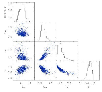
Figure 3.— Results from bootstrap Monte Carlo fits to 1000 realizations for Abell 1835 with A10 values for $\alpha$ and $\beta$. Here we can determine the scatter in each of the fitted gNFW parameters. $S_{90}$ is the flux density at 90 GHz as determined by MUSTANG.

If we simply append the MUSTANG model array to the Bolocam model array:

$$\overrightarrow{d}_{m}=[\overrightarrow{d}_{m,Bolocam},\overrightarrow{d}_{m,MUSTANG}]$$ (8)

then solving this set of equations would be a linear problem. However, we add a calibration offset term, $k$, to allow for offsets in calibration between MUSTANG and Bolocam data, and create the following array:

$$\overrightarrow{d}_{m,cal}=[\overrightarrow{d}_{m,Bolocam},k*\overrightarrow{d}_{m,MUSTANG}]$$ (9)

We cast Equation 9 as such because we expect the normalization given by MUSTANG and Bolocam to be equal, except for any calibration offset between instruments. Furthermore, we can quantify the calibration uncertainties and thus put a prior on it. Solving Equation 6 is no longer a problem of linearly independent variables. Thus, we use MPFIT to quickly solve for $\overrightarrow{a}_{m}$ and obtain a pseudo-$\chi^{2}$ ($\tilde{\chi}^{2}$). To calculate $\tilde{\chi}^{2}$, we use the same formulation as above, but redefine

$$\overrightarrow{d}_{cal} =[\overrightarrow{d}_{old},0.0]$$

$$\overrightarrow{d}_{m,cal} =[\overrightarrow{d}_{m,old},k]=\mathbf{A}_{new}\overrightarrow{a}_{m,cal}$$

where $\overrightarrow{a}_{m,cal}=[\overrightarrow{a}_{m},k]$, and expand $\mathbf{N}$ to allow for the extra fitted value. $\mathbf{N}$ is modified simply by assigning zero for all off-diagonal terms, and adding the expected variance of $k$ on the diagonal term. We adopt a calibration uncertainty of 11.2%, which accounts for the calibration accuracies of Bolocam and MUSTANG cited in Section 2.2.

3.5. Uncertainties

Figure 4.— Confidence intervals for Abell 1835 for A10 values of $\alpha$ and $\beta$. Top panel shows the confidence intervals for Bolocam only fit. Bottom panel shows the confidence intervals for the joint fit. Dashed lines show confidence intervals based on $\Delta\tilde{\chi}^{2}$. Solid lines are the true confidence intervals based on the bootstrap MC results. The asterisks denote the best fit.

For each set of fixed $\alpha$ and $\beta$ (see Table 3), the joint fit procedure returns a $\tilde{\chi}^{2}$. This is used to plot contours of $\Delta\tilde{\chi}^{2}$, and the equivalent confidence intervals. Following Sayers et al. (2011), the uncertainty for each parameter is estimated via the 1$\sigma$ confidence interval of the best fits over 1000 noise realizations added to model clusters. Furthermore, because $k$ is not an independent parameter, $\tilde{\chi}^{2}$ will not provide a fully accurate assessment of the confidence intervals.

We create 1000 realizations about the best fit model by adding 1000 instances of noise (for both Bolocam and MUSTANG) to the best fit model. Then, we find the best fit to each realization. The results of these fits is shown in Figure 3. The noise realizations for Bolocam are precomputed from previous work (Sayers et al., 2013). Noise realizations for MUSTANG are computed by random number generation with Gaussian distribution for each pixel, with $\sigma_{i}=\sqrt{1/w_{i}}$, based on the same weight used to calculate the noise matrix. These fits are tabulated and used to rescale the $\Delta\tilde{\chi}^{2}$ confidence intervals as seen in Figure 4. The rescaling of the confidence intervals is primarily due to the non-diagonality of the noise in the Bolocam covariance matrix.

We also investigated the potential impact from the uncertainty in the point source. For a given cluster, we follow the steps in Section 3.2, and we then calculate point source uncertainty models which adopt the $1\sigma$ values for the width of the main beam, as reported in Section 2.3, and fit the remaining components. The fitting procedure is then rerun twice: once with each of these models. Neither the fitted gNFW parameters nor the confidence intervals change. However, across the three point source models (two uncertainty and best-fit point source models), the minimum $\tilde{\chi}^{2}$ does change in the expected manner: it is greater for both of the uncertainty models than the best fit point source model.

4. Results

4.1. Abell 1835 (z=0.25)

Abell 1835 is a well studied massive cool core cluster. The cool core was noted to have substructure in the central $10\mbox{${}^{\prime\prime}$}$ by Schmidt et al. (2001), and identified as being due the central AGN by McNamara et al. (2006). Abell 1835 has also been extensively studied via the SZE (Reese et al., 2002; Benson et al., 2004; Bonamente et al., 2006; Sayers et al., 2011; Mauskopf et al., 2012). The models adopted were either beta models or generalized beta models, and tend to suggest a shallow slope for the pressure interior to $10\mbox{${}^{\prime\prime}$}$. Previous analysis of Abell 1835 with MUSTANG data (Korngut et al., 2011) detected the SZE decrement, but not at high significance, which is consistent with a featureless, smooth, broad signal. Our updated MUSTANG reduction of Abell 1835 is shown in Figure 5, and shows the same features as in Korngut et al. (2011).

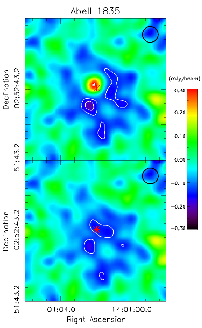
Figure 5.— MUSTANG SZE specific flux density map of Abell 1835. The white contours are at the 3 and 4 $\sigma$ significance level. The ACCEPT centroid is the red asterisk. The positive region close to the asterisk is the point source. The black circle in the upper right represents the effective beam of FWHM of $13.5\mbox{${}^{\prime\prime}$}$ (i.e. our $9\mbox{${}^{\prime\prime}$}$ telescope beam, smoothed by a $10\mbox{${}^{\prime\prime}$}$ FWHM Gaussian.)

Table 4Best fit gNFW parameters for Abell 1835

Model	$C_{500}$	$\alpha$	$\beta$	$\gamma$	$P_{0}$	k	$\tilde{\chi}^{2}$
N07	$1.44_{-0.22}^{+0.71}$	1.30	4.30	$0.74_{-0.13}^{+0.15}$	$3.43_{-1.78}^{+1.41}$	1.18	12837
A10	$0.83_{-0.15}^{+0.35}$	1.05	5.49	$0.75_{-0.17}^{+0.14}$	$2.54_{-1.37}^{+1.25}$	1.15	12835
P12	$1.45_{-0.28}^{+0.35}$	1.33	4.13	$0.84_{-0.12}^{+0.18}$	$2.80_{-1.15}^{+1.54}$	1.14	12838
S13	$2.29_{-0.52}^{+1.30}$	0.86	3.67	$0.36_{-0.21}^{+0.33}$	$19.3_{-6.16}^{+9.75}$	1.19	12831

Note. — $\gamma$, $P_{0}$, $C_{500}$, and k, the calibration offset, were varied. The degrees of freedom were 12880.

We find the best fit A10 model (all parameters but $P_{0}$ fixed to A10 values) has $\tilde{\chi}^{2}=12861$. To calculate $\tilde{\chi}^{2}$ for no cluster model, we fix the point source amplitude to that found in the previous fit. We find $\Delta\tilde{\chi}^{2}=892.1$, with $\Delta$DOF$=2$ corresponds to $29.7\sigma$ significance. For Bolocam only, the $\Delta\chi^{2}$ between a cluster model being fit or not yields a $28.9\sigma$ detection, while the for MUSTANG we find a $10.2\sigma$ detection of an A10 model from $\Delta\chi^{2}$.

Our best joint fit over the four sets of $\alpha$ and $\beta$, shown in Table 4, comes from the S13 values of $\alpha$ and $\beta$: the best fit floated parameters are: $\gamma=0.36$, $P_{0}=19.3$, and $C_{500}=2.28$. Despite variations in the best fit $\gamma$ values, Figure 6 shows the best joint fit pressure profiles of Abell 1835 for each of the four sets of fixed $\alpha$ and $\beta$, are in good agreement with each other. Moreover, we find that the four model fits achieve minimum scatter at two separate radii, roughly corresponding to the geometric mean between the resolution and FOV of each instrument.

We find the point source in the MUSTANG map at R.A.=14:01:02.1, Dec=02:52:47 is best fit with a flux density of $1.38\pm 0.10$ mJy, and has a correlation coefficient of 0.076 with the cluster amplitude. This minimal degeneracy can also be seen in Figure 3. Similarly, changing the assumed beam shape as discussed in Section 3.5 has a negligible change on the flux density. The amplitude of the point source suggests a slight flattening of the spectral index between $\nu=1.4$ GHz and $\nu=28.5$ GHz (Condon et al. (1998),Reese et al. (2002)) of $\alpha_{\nu}=0.89$, to a spectral index of $\alpha_{\nu}=0.59$ between $\nu=28.5$ GHz and $\nu=90$ GHz. Such a spectral index is also consistent with McNamara et al. (2014), which find a spectral index of $\alpha_{\nu}=0.54$ between $\nu=92$ GHz and $\nu=276$ GHz. The assumed flux density of the subtracted point source for Bolocam, $0.77\pm 0.24$ mJy at 140 GHz, is consistent with the other measurements.

The point source flux density found with MUSTANG is consistent with that obtained from observations with the Atacama Large Millimeter/Sub-millimeter Array (ALMA) in McNamara et al. (2014), which find the central continuum source has a flux density of 1.26 $\pm 0.03$ mJy. We note they also detect a $10^{10}M_{\odot}$ molecular outflow at 92 GHz, with a total integral flux of $3.6$ Jy km s^-1 for CO (1-0), which would correspond to an equivalent continuum flux density of 6 $\mu$Jy, and would not contribute much additional flux density to the point source flux density as seen by McNamara et al. (2014). However, this source is reported with a position of R.A.=14:01:02.083, Dec=02:52:42.649, which is $4\mbox{${}^{\prime\prime}$}$ offset from the position found in our MUSTANG data. Since we consider our positional uncertainty to be $2\mbox{${}^{\prime\prime}$}$, this is a larger than typical pointing offset, but is difficult to rule out. A list of selected point source flux densities is provided in Table 4.1.

Figure 4 shows that Bolocam, by itself, can place fairly tight constraints on the gNFW model parameters, primarily on $C_{500}$. That is, for A10 values of $\alpha$ and $\beta$, as in Figure 4, Bolocam finds $C_{500}=0.73_{-0.17}^{+0.25}$, $\gamma=0.83_{-0.23}^{+0.22}$, and $P_{0}=1.75_{-1.22}^{+2.51}$, whereas the joint fit yields $C_{500}=0.83_{-0.15}^{+0.35}$, $\gamma=0.75_{-0.17}^{+0.14}$, and $P_{0}=2.54_{-1.37}^{+1.25}$. Across the model sets, the trend for Abell 1835 is that joint fit tends to loosen the constraint on $C_{500}$, while improving the constraints on $\gamma$ and $P_{0}$ relative to the fits to solely Bolocam data. It is worth noting that for each value of $\gamma$ and $C_{500}$, only $P_{0}$ is a free parameter in the Bolocam only fits. In contrast, for the joint fit, the calibration offset and MUSTANG point source amplitude are additional free parameters. The addition of MUSTANG data slightly reduces the inner slope, $\gamma$, relative to the Bolocam-only fit. This is suggestive that Bolocam, with subtraction of its adopted point source model, has not underestimated the SZE signal. Moreover, given the peak decrement of $-20$ mJy in the Bolocam map, an adjustment of $\sim 0.2$ mJy, which is the uncertainty on the assumed $0.77$ mJy, would negligibly alter the constraints. Both the Bolocam and joint constraints indicate a relatively steep slope, which is typical for a cool core cluster (e.g. Arnaud et al., 2010; Sayers et al., 2013).

Table 5Abell 1835 point source flux densities

$S_{1.4}^{a}$ (mJy)	$S_{28.5}^{b}$ (mJy)	$S_{90}$ (mJy)	$S_{92}^{c}$ (mJy)	$S_{276}^{c}$ (mJy)
$41.4\pm 1.9$	$2.76\pm 0.14$	$1.38\pm 0.10$	$1.26\pm 0.03$	$0.7\pm 0.1$

Note. — $S_{90}$ is from this work.

References. — ^a From Condon et al. (1998) ^b From Reese et al. (2002) ^c From McNamara et al. (2014).

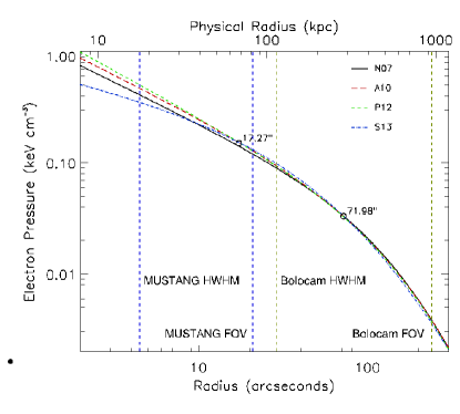
Figure 6.— Best fit pressure profiles for Abell 1835 for the different sets of fixed $\alpha$ and $\beta$, denoted by the model it is taken from. The circles denote radial ranges where the pressure profiles show (local) minimum scatter.

4.2. MACS J0647.7+7015 (z=0.59)

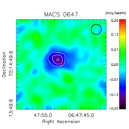
Figure 7.— MUSTANG SZE flux density map of MACS 0647. The white contours are at the 3, 4, and 5 $\sigma$ significance level. The ACCEPT centroid is the red asterisk. The black circle in the upper right represents the effective beam of FWHM of $13.5\mbox{${}^{\prime\prime}$}$.

MACS 0647 is at $z=0.591$ and is classified as neither a cool core nor a disturbed cluster (Sayers et al., 2013). It was included in the CLASH sample due to its strong lensing properties (Postman et al., 2012). Gravitational lensing (Zitrin et al., 2011), X-ray surface brightness (Mann & Ebeling, 2012), and SZE (MUSTANG, see Figure 7, and Bolocam) maps all show elongation in an east-west direction. In the joint analysis presented here, we see that the spherical model provides an adequate fit to both datasets and we note that the spherical assumption allows for a easier interpretation of the mass profile of the cluster.

To calculate how significantly Bolocam and MUSTANG detect an SZE bulk decrement, we calculate a $\Delta\tilde{\chi}^{2}$ as we did for Abell 1835. $\Delta\tilde{\chi}^{2}$ is computed as the difference of $\tilde{\chi}^{2}$ from an A10 profile (all parameters but $P_{0}$ fixed to A10 values) fit to our datasets, and $\tilde{\chi}^{2}$ assuming no model. The joint fit (both data sets) yields a $26.3\sigma$ significance, while for Bolocam only, $\Delta\chi^{2}$ yields a $23.9\sigma$ detection, and in the MUSTANG data we find a $10.8\sigma$ detection of an A10 model.

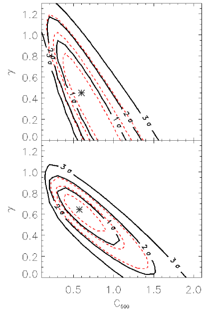
Figure 8.— Confidence intervals for MACS 0647 with A10 values of $\alpha$ and $\beta$. Top panel shows the confidence intervals for Bolocam only fit. Bottom panel shows the confidence intervals for the joint fit. Dashed lines show confidence intervals based on $\Delta\tilde{\chi}^{2}$ at face value. Solid lines are the true confidence intervals based on the bootstrap MC results.

Table 6Best fit gNFW parameters for MACS 0647

Model	$C_{500}$	$\alpha$	$\beta$	$\gamma$	$P_{0}$	$k$	$\tilde{\chi^{2}}$
N07	$0.93_{-0.36}^{+0.31}$	1.30	4.30	$0.70_{-0.17}^{+0.10}$	$2.10_{-1.17}^{+0.93}$	1.14	12845
A10	$0.60_{-0.22}^{+0.25}$	1.05	5.49	$0.61_{-0.15}^{+0.12}$	$2.24_{-1.20}^{+2.03}$	1.14	12844
P12	$1.03_{-0.40}^{+0.32}$	1.33	4.13	$0.70_{-0.17}^{+0.10}$	$2.25_{-1.32}^{+1.04}$	1.14	12845
S13	$1.19_{-0.64}^{+0.54}$	0.86	3.67	$0.38_{-0.25}^{+0.20}$	$8.18_{-1.13}^{+4.68}$	1.14	12843

Note. — $\gamma$, $P_{0}$, and $C_{500}$ were varied. The degrees of freedom were 12914.

Our best fit model comes from the S13 values of $\alpha$ and $\beta$, and finds $\gamma=0.38$, $C_{500}=1.19$, and $P_{0}=8.18$. The best joint fits, listed in Table 6 to the four sets of $\alpha$ and $\beta$ differ by $\Delta\tilde{\chi^{2}}<3$. With Young et al. (2014) constraining $\gamma=0.90_{-0.04}^{+0.02}$, it might appear that their result is significantly discrepant with our best fit $\gamma=0.61_{-0.11}^{+0.17}$ from the A10 set, even though Young et al. (2014) used the identical SZE data as we have used in this analysis. A crucial distinction in the fitting procedures is the parameter space searched: in Young et al. (2014), Bolocam is first fit over grid of fixed $\gamma$ values, $k$ is fixed at 1.0, and the parameters $C_{500}$ and $P_{0}$ are allowed to float. The resultant fits for each $\gamma$ are then fit as-is (nothing allowed to float) to the MUSTANG map. Thus, the reported error bars reflect a one-parameter search, without the degeneracies between $C_{500}$, $P_{0}$, and $\gamma$ folded into it, and do not include the $\chi^{2}$ values from the Bolocam fit.

Given that MUSTANG is only able to constrain the pressure profile on scales $9\mbox{${}^{\prime\prime}$}<\theta\lesssim 42\mbox{${}^{\prime\prime}$}$, and for MACS 0647, $R_{500}=3.16$^′and $C_{500}=1.18$ (A10 and S13 value) or $C{500}=1.8$ (N07 and P12 value), then $\beta$ should not relate to the slope within the scales probed by MUSTANG. It is possible for $\alpha$ to relate to the slope within the scales in question. However, As $C_{500}$ decrease, especially below 1.0, as is the case in both this work and Young et al. (2014), then $\alpha$ will relate less to the slope within the scales probed by MUSTANG. Crucially, that cluster pressure profile steepen with increasing radius gives rise to the degeneracy observed between $C_{500}$ and $\gamma$ as seen in Figures 4 and 8.

Figure 8 shows that Bolocam does not place strong constraints on $\gamma$ and $C_{500}$, especially relative to the joint fit (Table 6). Specifically, for the A10 set of $\alpha$ and $\beta$, the Bolocam finds $C_{500}=0.66_{-0.38}^{+0.34}$, $\gamma=0.39_{-0.39}^{+0.49}$, and $P_{0}=17.7_{-8.27}^{+2.76}$. As in Figure 6, we see in Figure 9 that the best joint fit pressure profiles from the different gNFW fits of MACS 0647 are in good agreement, and the radii where Bolocam and MUSTANG have the tightest constraints are similar to the radii of tightest constraints found in Abell 1835. Figure 10 shows the two-dimensional confidence intervals over the parameter space searched for MACS 0647.

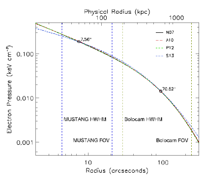
Figure 9.— Best fit pressure profiles for MACS 0647 for the different sets of fixed gNFW $\alpha$ and $\beta$, denoted by the model the values are taken from. The circles denote radial ranges where the pressure profiles show (local) minimum scatter.

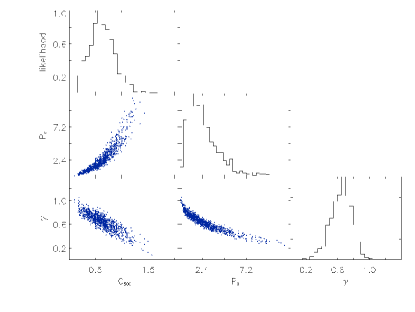
Figure 10.— Results from Monte Carlo fits to 1000 realizations for MACS 0647 with A10 values for $\alpha$ and $\beta$.

4.3. Comparison with ACCEPT

ACCEPT (Cavagnolo et al., 2009) utilizes the Chandra Data Archive (CDA) to derive entropy (and pressure) profiles for 239 galaxy clusters. We summarize how Cavagnolo et al. calculate pressure profiles here. ACCEPT pressure profiles are calculated as the product of their derived temperature and electron density profiles. All the ACCEPT data pulled from CDA for ACCEPT were taken with the ACIS detectors (Garmire et al., 2003). Cavagnolo et al. first derive temperature profiles from spectra. The spectra are fitted from annuli containing at least 2500 counts after background subtraction. Electron density is then calculated from surface brightness profiles using the 0.7-2.0 keV range. This time, annuli of $5\mbox{${}^{\prime\prime}$}$ are used (pixels are $0.\mbox{${}^{\prime\prime}$}492$). To account for the slight temperature dependence of X-ray surface brightness, an appropriate temperature for each surface brightness annulus is interpolated from the radial temperature profile grid.

We see in Figures 11 and 12 that our joint fits of SZE observations agree well with ACCEPT data. We note that the ACCEPT profiles show some deviation from a gNFW curve. For Abell 1835, there is a bump in the pressure at $r\sim 40\mbox{${}^{\prime\prime}$}$. In MACS 0647, from $r\sim 15\mbox{${}^{\prime\prime}$}$ to $r\sim 100\mbox{${}^{\prime\prime}$}$, the ACCEPT pressure profile is almost a pure power law.

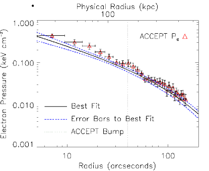
Figure 11.— Pressure profiles for Abell 1835. The dotted lines show the $1\sigma$ error bars on the SZE determined pressure profile. The best joint fit from this work is the solid line. ACCEPT error bars are at the 90% confidence level.

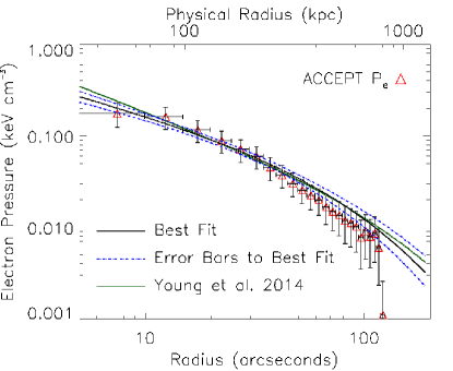
Figure 12.— Pressure profiles for MACS 0647. The best fit (this work) is the solid black line, the dashed lines show the $1\sigma$ error bars from the joint fit, and the solid dark green is the best fit found in Young et al. 2014. ACCEPT error bars are at the 90% confidence level.

5. Discussion

Here we have presented an approach to jointly fit models to SZE data from different instruments. With regards to our current sample, we have shown that this approach finds pressure profiles that are in good agreement with X-ray derived pressure profiles. We choose to vary gNFW parameters that correspond to the central regions ($P_{0}$, $C_{500}$, and $\gamma$) given that we expect our data will be best suited to constraining these, and to avoid encountering the large degeneracy between all the parameters.

In Abell 1835 and MACS0647 standard A10 models are detected at 29.7$\sigma$ and 26.3$\sigma$ significance respectively. For Abell 1835, our best fit is $\gamma=0.36_{-0.36}^{+0.18}$, $C_{500}=2.29_{-0.68}^{+0.27}$, and $P_{0}=19.3_{-8.53}^{+20.4}$ with fixed values of $\alpha=0.86$ and $\beta=3.67$ from S13. For MACS 0647, our best fit is $\gamma=0.38_{-0.25}^{+0.20}$, $C_{500}=1.19_{-0.64}^{+0.54}$, and $P_{0}=8.18_{-1.13}^{+4.68}$ with fixed values of $\alpha=0.86$ and $\beta=3.67$ from S13. The error bars have been calculated via 1000 Monte Carlo realizations and are marginalized over the other parameters. While the spread in fitted parameters appear large (e.g. in Abell 1835, we find $\gamma=0.36$ with S13 values of $\alpha$ and $\beta$, and we find $\gamma=0.84$ for P12 values of $\alpha$ and $\beta$), we note that the fitted pressure profiles are in very good agreement (Figures 6 and 9), and the profiles reveal nodes of least scatter set by MUSTANG and Bolocam. These two nodes occur roughly where expected: at the geometric mean each instrument’s resolution and FOV.

With this approach, we find that contaminants such as point sources can be well modeled and their amplitudes are minimally degenerate with cluster pressure models. The pressure profile constraints do not depend on the MUSTANG beam shape assumed to model point sources. Furthermore, we find joint fits with MUSTANG and Bolocam allow tight constraints on the pressure profiles over a large range of scales.

Confidence intervals for both MACS 0647 and Abell 1835 show that the constraints are weaker than indicated from $\tilde{\chi}^{2}$. This discrepancy arises because the true covariance matrix for Bolocam is not diagonal, as assumed for individual fits.

Abell 1835 and MACS 0647 also illustrate the importance of spanning a range of angular scales. While Bolocam data alone provide good constraints on $\gamma$ and $C_{500}$ for Abell 1835, Bolocam data do not provide precise constraints on these parameters for MACS 0647. While data quality and quantity may explain some of the difference, a critical distinction is that $R_{500}$ occurs at $6.30\arcmin$ for Abell 1835, and $3.16\arcmin$ for MACS 0647, which is primarily due to Abell 1835 being at lower redshift ($z=0.253$) than MACS 0647 ($z=0.591$). The inner pressure profile of Abell 1835 can be constrained by Bolocam, but due to its larger angular extent, MUSTANG will filter out much ($r>1\arcmin$) of the profile within $R_{500}$. However, MACS 0647 appears smaller on the sky and higher resolution (than $58\mbox{${}^{\prime\prime}$}$) is necessary to constrain the inner pressure profile. Therefore, the addition of high resolution MUSTANG data becomes crucial for clusters at large redshifts.

A significant improvement to this approach would be to reduce the computational resources required. Currently, the forward filtering of our MUSTANG models is the most computationally expensive step. As this step is required for each model created, this restricts how many models we can produce, and thus it restricts the parameter space we can search. Computing a transfer function for MUSTANG would significantly reduce the total computational expense; however, the applicability of such a transfer function must be assessed.

We plan to expand this joint fitting technique to a larger sample of clusters, and we note that both Bolocam and MUSTANG show good internal consistency in their flux calibration. As a result, a single value of $k$ should be valid for all of the clusters observed by both instruments, and therefore we expect it can be tightly constrained using the full sample. This will effectively eliminate one of the free parameters in our fits, and produce tighter constraints on the gNFW model parameters.

References

- Abramopoulos et al. (1981) Abramopoulos, F., Chanan, G. A., & Ku, W. H.-M. 1981, ApJ, 248, 429
- Arnaud et al. (2010) Arnaud, M., Pratt, G. W., Piffaretti, R., Böhringer, H., Croston, J. H., & Pointecouteau, E. 2010, A&A, 517, A92
- Battaglia et al. (2012) Battaglia, N., Bond, J. R., Pfrommer, C., & Sievers, J. L. 2012, ApJ, 758, 75
- Benson et al. (2004) Benson, B. A., Church, S. E., Ade, P. A. R., Bock, J. J., Ganga, K. M., Henson, C. N., & Thompson, K. L. 2004, ApJ, 617, 829
- Bonamente et al. (2012) Bonamente, M., Hasler, N., Bulbul, E., Carlstrom, J. E., Culverhouse, T. L., Gralla, M., Greer, C., Hawkins, D., Hennessy, R., Joy, M., Kolodziejczak, J., Lamb, J. W., Landry, D., Leitch, E. M., Marrone, D. P., Miller, A., Mroczkowski, T., Muchovej, S., Plagge, T., Pryke, C., Sharp, M., & Woody, D. 2012, New Journal of Physics, 14, 025010
- Bonamente et al. (2006) Bonamente, M., Joy, M. K., LaRoque, S. J., Carlstrom, J. E., Reese, E. D., & Dawson, K. S. 2006, ApJ, 647, 25
- Borgani et al. (2004) Borgani, S., Murante, G., Springel, V., Diaferio, A., Dolag, K., Moscardini, L., Tormen, G., Tornatore, L., & Tozzi, P. 2004, MNRAS, 348, 1078
- Carlstrom et al. (2002) Carlstrom, J. E., Holder, G. P., & Reese, E. D. 2002, ARA&A, 40, 643
- Cavagnolo et al. (2009) Cavagnolo, K. W., Donahue, M., Voit, G. M., & Sun, M. 2009, ApJS, 182, 12
- Condon et al. (1998) Condon, J. J., Cotton, W. D., Greisen, E. W., Yin, Q. F., Perley, R. A., Taylor, G. B., & Broderick, J. J. 1998, AJ, 115, 1693
- Czakon et al. (2014) Czakon, N. G., Sayers, J., Mantz, A., Golwala, S. R., Downes, T. P., Koch, P. M., Lin, K.-Y., Molnar, S. M., Moustakas, L. A., Mroczkowski, T., Pierpaoli, E., Shitanishi, J. A., Siegel, S., & Umetsu, K. 2014, ArXiv e-prints 1406.2800
- Dicker et al. (2008) Dicker, S. R., Korngut, P. M., Mason, B. S., Ade, P. A. R., Aguirre, J., Ames, T. J., Benford, D. J., Chen, T. C., Chervenak, J. A., Cotton, W. D., Devlin, M. J., Figueroa-Feliciano, E., Irwin, K. D., Maher, S., Mello, M., Moseley, S. H., Tally, D. J., Tucker, C., & White, S. D. 2008, in Society of Photo-Optical Instrumentation Engineers (SPIE) Conference Series, Vol. 7020, Society of Photo-Optical Instrumentation Engineers (SPIE) Conference Series
- Ebeling et al. (2007) Ebeling, H., Barrett, E., Donovan, D., Ma, C.-J., Edge, A. C., & van Speybroeck, L. 2007, ApJ, 661, L33
- Ebeling et al. (2010) Ebeling, H., Edge, A. C., Mantz, A., Barrett, E., Henry, J. P., Ma, C. J., & van Speybroeck, L. 2010, MNRAS, 407, 83
- Fabian et al. (2006) Fabian, A. C., Sanders, J. S., Taylor, G. B., Allen, S. W., Crawford, C. S., Johnstone, R. M., & Iwasawa, K. 2006, MNRAS, 366, 417
- Garmire et al. (2003) Garmire, G. P., Bautz, M. W., Ford, P. G., Nousek, J. A., & Ricker, Jr., G. R. 2003, in Society of Photo-Optical Instrumentation Engineers (SPIE) Conference Series, Vol. 4851, X-Ray and Gamma-Ray Telescopes and Instruments for Astronomy., ed. J. E. Truemper & H. D. Tananbaum, 28–44
- Gilfanov & Syunyaev (1984) Gilfanov, M. R. & Syunyaev, R. A. 1984, Soviet Astronomy Letters, 10, 137
- Glenn et al. (1998) Glenn, J., Bock, J. J., Chattopadhyay, G., Edgington, S. F., Lange, A. E., Zmuidzinas, J., Mauskopf, P. D., Rownd, B., Yuen, L., & Ade, P. A. 1998, Proc. SPIE, 3357, 326
- Haig et al. (2004) Haig, D. J., Ade, P. A. R., Aguirre, J. E., Bock, J. J., Edgington, S. F., Enoch, M. L., Glenn, J., Goldin, A., Golwala, S., Heng, K., Laurent, G., Maloney, P. R., Mauskopf, P. D., Rossinot, P., Sayers, J., Stover, P., & Tucker, C. 2004, in Society of Photo-Optical Instrumentation Engineers (SPIE) Conference Series, Vol. 5498, Society of Photo-Optical Instrumentation Engineers (SPIE) Conference Series, ed. C. M. Bradford, P. A. R. Ade, J. E. Aguirre, J. J. Bock, M. Dragovan, L. Duband, L. Earle, J. Glenn, H. Matsuhara, B. J. Naylor, H. T. Nguyen, M. Yun, & J. Zmuidzinas, 78–94
- Hinshaw et al. (2013) Hinshaw, G., Larson, D., Komatsu, E., Spergel, D. N., Bennett, C. L., Dunkley, J., Nolta, M. R., Halpern, M., Hill, R. S., Odegard, N., Page, L., Smith, K. M., Weiland, J. L., Gold, B., Jarosik, N., Kogut, A., Limon, M., Meyer, S. S., Tucker, G. S., Wollack, E., & Wright, E. L. 2013, ApJS, 208, 19
- Jewell & Prestage (2004) Jewell, P. R. & Prestage, R. M. 2004, in Society of Photo-Optical Instrumentation Engineers (SPIE) Conference Series, Vol. 5489, Ground-based Telescopes, ed. J. M. Oschmann, Jr., 312–323
- Korngut et al. (2011) Korngut, P. M., Dicker, S. R., Reese, E. D., Mason, B. S., Devlin, M. J., Mroczkowski, T., Sarazin, C. L., Sun, M., & Sievers, J. 2011, ApJ, 734, 10
- Kravtsov & Borgani (2012) Kravtsov, A. V. & Borgani, S. 2012, ARA&A, 50, 353
- Mann & Ebeling (2012) Mann, A. W. & Ebeling, H. 2012, MNRAS, 420, 2120
- Mantz et al. (2010) Mantz, A., Allen, S. W., Rapetti, D., & Ebeling, H. 2010, MNRAS, 406, 1759
- Markevitch & Vikhlinin (2007) Markevitch, M. & Vikhlinin, A. 2007, Phys. Rep., 443, 1
- Markwardt (2009) Markwardt, C. B. 2009, in Astronomical Society of the Pacific Conference Series, Vol. 411, Astronomical Data Analysis Software and Systems XVIII, ed. D. A. Bohlender, D. Durand, & P. Dowler, 251
- Mauskopf et al. (2012) Mauskopf, P. D., Horner, P. F., Aguirre, J., Bock, J. J., Egami, E., Glenn, J., Golwala, S. R., Laurent, G., Nguyen, H. T., & Sayers, J. 2012, MNRAS, 421, 224
- McNamara & Nulsen (2007) McNamara, B. R. & Nulsen, P. E. J. 2007, ARA&A, 45, 117
- McNamara et al. (2006) McNamara, B. R., Rafferty, D. A., Bîrzan, L., Steiner, J., Wise, M. W., Nulsen, P. E. J., Carilli, C. L., Ryan, R., & Sharma, M. 2006, ApJ, 648, 164
- McNamara et al. (2014) McNamara, B. R., Russell, H. R., Nulsen, P. E. J., Edge, A. C., Murray, N. W., Main, R. A., Vantyghem, A. N., Combes, F., Fabian, A. C., Salome, P., Kirkpatrick, C. C., Baum, S. A., Bregman, J. N., Donahue, M., Egami, E., Hamer, S., O’Dea, C. P., Oonk, J. B. R., Tremblay, G., & Voit, G. M. 2014, ApJ, 785, 44
- Mroczkowski et al. (2009) Mroczkowski, T., Bonamente, M., Carlstrom, J. E., Culverhouse, T. L., Greer, C., Hawkins, D., Hennessy, R., Joy, M., Lamb, J. W., Leitch, E. M., Loh, M., Maughan, B., Marrone, D. P., Miller, A., Muchovej, S., Nagai, D., Pryke, C., Sharp, M., & Woody, D. 2009, ApJ, 694, 1034
- Nagai et al. (2007) Nagai, D., Kravtsov, A. V., & Vikhlinin, A. 2007, ApJ, 668, 1
- Navarro et al. (1997) Navarro, J. F., Frenk, C. S., & White, S. D. M. 1997, ApJ, 490, 493
- Nelson et al. (2014) Nelson, K., Lau, E. T., & Nagai, D. 2014, ApJ, 792, 25
- Nikolic et al. (2007) Nikolic, B., Prestage, R. M., Balser, D. S., Chandler, C. J., & Hills, R. E. 2007, A&A, 465, 685
- Peng & Nagai (2009) Peng, F. & Nagai, D. 2009, ApJ, 693, 839
- Peterson et al. (2001) Peterson, J. R., Paerels, F. B. S., Kaastra, J. S., Arnaud, M., Reiprich, T. H., Fabian, A. C., Mushotzky, R. F., Jernigan, J. G., & Sakelliou, I. 2001, A&A, 365, L104
- Planck Collaboration et al. (2013) Planck Collaboration, Ade, P. A. R., Aghanim, N., Arnaud, M., Ashdown, M., Atrio-Barandela, F., Aumont, J., Baccigalupi, C., Balbi, A., Banday, A. J., & et al. 2013, A&A, 558, C2
- Postman et al. (2012) Postman, M., Coe, D., Benítez, N., Bradley, L., Broadhurst, T., Donahue, M., Ford, H., Graur, O., Graves, G., Jouvel, S., Koekemoer, A., Lemze, D., Medezinski, E., Molino, A., Moustakas, L., Ogaz, S., Riess, A., Rodney, S., Rosati, P., Umetsu, K., Zheng, W., Zitrin, A., Bartelmann, M., Bouwens, R., Czakon, N., Golwala, S., Host, O., Infante, L., Jha, S., Jimenez-Teja, Y., Kelson, D., Lahav, O., Lazkoz, R., Maoz, D., McCully, C., Melchior, P., Meneghetti, M., Merten, J., Moustakas, J., Nonino, M., Patel, B., Regös, E., Sayers, J., Seitz, S., & Van der Wel, A. 2012, ApJS, 199, 25
- Reese et al. (2002) Reese, E. D., Carlstrom, J. E., Joy, M., Mohr, J. J., Grego, L., & Holzapfel, W. L. 2002, ApJ, 581, 53
- Sayers et al. (2013) Sayers, J., Czakon, N. G., Mantz, A., Golwala, S. R., Ameglio, S., Downes, T. P., Koch, P. M., Lin, K.-Y., Maughan, B. J., Molnar, S. M., Moustakas, L., Mroczkowski, T., Pierpaoli, E., Shitanishi, J. A., Siegel, S., Umetsu, K., & Van der Pyl, N. 2013, ApJ, 768, 177
- Sayers et al. (2011) Sayers, J., Golwala, S. R., Ameglio, S., & Pierpaoli, E. 2011, ApJ, 728, 39
- Schmidt et al. (2001) Schmidt, R. W., Allen, S. W., & Fabian, A. C. 2001, MNRAS, 327, 1057
- Shaw et al. (2010) Shaw, L. D., Nagai, D., Bhattacharya, S., & Lau, E. T. 2010, ApJ, 725, 1452
- Sunyaev & Zel’dovich (1972) Sunyaev, R. A. & Zel’dovich, Y. B. 1972, Comments Astrophys. Space Phys., 4, 173
- Vikhlinin et al. (2006) Vikhlinin, A., Kravtsov, A., Forman, W., Jones, C., Markevitch, M., Murray, S. S., & Van Speybroeck, L. 2006, ApJ, 640, 691
- Weiland et al. (2011) Weiland, J. L., Odegard, N., Hill, R. S., Wollack, E., Hinshaw, G., Greason, M. R., Jarosik, N., Page, L., Bennett, C. L., Dunkley, J., Gold, B., Halpern, M., Kogut, A., Komatsu, E., Larson, D., Limon, M., Meyer, S. S., Nolta, M. R., Smith, K. M., Spergel, D. N., Tucker, G. S., & Wright, E. L. 2011, ApJS, 192, 19
- Young et al. (2014) Young, A. H., Mroczkowski, T., Romero, C., Sayers, J., Balestra, I., Clarke, T. E., Czakon, N., Devlin, M., Dicker, S. R., Ferrari, C., Girardi, M., Golwala, S., Intema, H., Korngut, P. M., Mason, B. S., Mercurio, A., Nonino, M., Reese, E. D., Rosati, P., Sarazin, C., & Umetsu, K. 2014, ArXiv e-prints 1411.0317
- Zitrin et al. (2011) Zitrin, A., Broadhurst, T., Barkana, R., Rephaeli, Y., & Benítez, N. 2011, MNRAS, 410, 1939