Better bounds for planar sets avoiding unit distances

Abstract.

A $1$-avoiding set is a subset of $\mathbb{R}^{n}$ that does not contain pairs of points at distance $1$. Let $m_{1}(\mathbb{R}^{n})$ denote the maximum fraction of $\mathbb{R}^{n}$ that can be covered by a measurable $1$-avoiding set. We prove two results. First, we show that any $1$-avoiding set in $\mathbb{R}^{n}$ ($n\geq 2$) that displays block structure (i.e., is made up of blocks such that the distance between any two points from the same block is less than $1$ and points from distinct blocks lie farther than $1$ unit of distance apart from each other) has density strictly less than $1/2^{n}$. For the special case of sets with block structure this proves a conjecture of Erdős asserting that $m_{1}(\mathbb{R}^{2})<1/4$. Second, we use linear programming and harmonic analysis to show that $m_{1}(\mathbb{R}^{2})\leq 0.258795$.

1. Introduction

The unit-distance graph of $\mathbb{R}^{n}$ is the graph whose vertex set is $\mathbb{R}^{n}$ and in which $x$ and $y$ are adjacent if $\|x-y\|=1$. A well-known problem in geometry, going back to Nelson and Hadwiger (see Soifer [12] for a historical survey), asks for the chromatic number $\chi(\mathbb{R}^{n})$ of the unit-distance graph of $\mathbb{R}^{n}$.

A related problem considers independent sets of the unit-distance graph. Let $G=(V,E)$ be a graph. A set $I\subseteq V$ is independent if it does not contain a pair of adjacent vertices. The independence number of $G$, denoted by $\alpha(G)$, is the maximal cardinality of an independent set.

A set $A\subseteq\mathbb{R}^{n}$ is independent in the unit-distance graph if it does not contain pairs of points at distance $1$, that is, $\|x-y\|\neq 1$ for all $x$, $y\in A$. We also say that $A$ avoids distance $1$ or that it is a $1$-avoiding set. A possible measure for the size of an independent set in this case is its density, that is, the fraction of space that it covers (see §1.1 for a rigorous definition). Our aim is to estimate the maximal (or more precisely the least upper bound of the) fraction of $\mathbb{R}^{n}$ that can be covered by a measurable set that avoids distance $1$.

We denote this maximal fraction by $m_{1}(\mathbb{R}^{n})$. In §3, we show that $m_{1}(\mathbb{R}^{2})\leq 0.258795$. This result is related to a conjecture of Erdős (cf. Székely [14]), stating that $m_{1}(\mathbb{R}^{2})<1/4$.

As for the chromatic number of the Euclidean plane, all that is known is that $4\leq\chi(\mathbb{R}^{2})\leq 7$. The upper bound comes from a simple periodic coloring of $\mathbb{R}^{2}$, whereas the lower bound comes from a finite subgraph of the unit-distance graph, the Moser spindle (cf. Moser and Moser [9]), whose chromatic number is $4$ (see Figure 1).

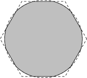
Figure 1. On the left, the Moser spindle [9]. Each segment has length exactly $1$. On the right, the optimal tortoise in Croft’s construction [2].

In view of the difficulty of computing $\chi(\mathbb{R}^{n})$, Falconer [3] introduced the measurable chromatic number, denoted by $\chi_{\rm m}(\mathbb{R}^{n})$, in which the restriction is added that the color classes must be Lebesgue-measurable sets. In other words, one wishes to partition $\mathbb{R}^{n}$ into the minimum possible number of Lebesgue-measurable $1$-avoiding sets. Obviously, $\chi_{\rm m}(\mathbb{R}^{n})\geq\chi(\mathbb{R}^{n})$. Falconer proved that $\chi_{\rm m}(\mathbb{R}^{2})\geq 5$. Since

$$m_{1}(\mathbb{R}^{n})\chi_{\rm m}(\mathbb{R}^{n})\geq 1,$$

showing Erdős’ conjecture would give another proof of Falconer’s result.

A simple lower bound for $m_{1}(\mathbb{R}^{2})$ comes from the following construction. Consider the hexagonal lattice with minimal vectors of length $2$ and place at each point of the lattice an open disk of radius $1/2$. This is a $1$-avoiding set of density $\pi/(8\sqrt{3})=0.2267\ldots$. A slight improvement was given by Croft [2]. His construction is as follows. Shrink the hexagonal lattice slightly so as to have minimal vectors of length $1+x$, where $x<1$, and place at each lattice point the intersection of an open disk of radius $1/2$ and an open regular hexagon of height $x$. The disks guarantee that inside each block every distance is less than $1$, while the hexagons guarantee that points from different blocks have distance greater than $1$. Taking $x=0.96553\ldots$ maximizes the density of the union of all the blocks, showing that $m_{1}(\mathbb{R}^{2})\geq 0.22936$. This intersection of a disk with a hexagon has often been called a tortoise; Figure 1 shows an optimal tortoise.

Any finite subgraph $G=(V,E)$ of the unit-distance graph of $\mathbb{R}^{n}$ provides an upper bound for $m_{1}(\mathbb{R}^{n})$, namely $\alpha(G)/|V|$; this can be seen via a simple averaging argument. For the plane, we then immediately have that $m_{1}(\mathbb{R}^{2})\leq 1/3$, as can be seen from the equilateral triangle. A better bound of $2/7$ is provided by the Moser spindle; this is the best upper bound that has been obtained from a finite subgraph.

Using further ideas, Székely [15] proved a bound of $\approx 0.279<2/7\approx 0.285$. Oliveira and Vallentin [10] gave the currently best known upper bound of $\approx 0.268$. Their method is based on a mix of linear programming and harmonic analysis; it is a strengthening of it that will be used in §3 to prove that $m_{1}(\mathbb{R}^{2})\leq 0.258795$.

Frankl and Wilson [4] construct finite subgraphs of the unit-distance graph of $\mathbb{R}^{n}$ whose chromatic numbers grow exponentially fast in $n$. These same subgraphs can be used to provide the asymptotic upper bound

$$m_{1}(\mathbb{R}^{n})\leq(1+o(1))1.207^{-n}.$$

via the averaging argument. The method of Oliveira and Vallentin [10] also provides an exponential upper bound, $m_{1}(\mathbb{R}^{n})\leq(1+o(1))1.1654^{-n}$, which is somewhat weaker than the bound of Frankl and Wilson. A combination of both arguments, requiring detailed analysis, was used by Bachoc, Passuello, and Thiery [1] to obtain the best known asymptotic upper bound

$$m_{1}(\mathbb{R}^{n})\leq(1+o(1))1.268^{-n}.$$

We remark here that the results of [1] and the present paper do not overlap: the authors of [1] obtain asymptotic upper bounds as $n\to\infty$, and some numerical improvements for dimensions $4\leq n\leq 24$.

The behavior of $\chi(\mathbb{R}^{n})$ under restrictions placed on the color classes has also been studied. We have already mentioned Falconer’s measurable chromatic number. Other restrictions include requiring all classes to be either open or closed sets — in both cases it can be shown that the chromatic number of $\mathbb{R}^{2}$ is either $6$ or $7$ (cf. Soifer [12]).

Similarly, we may place some natural restrictions on $1$-avoiding sets and study their maximal possible upper densities. In particular, we will consider sets with block structure. We say that a set $A$ has block structure if it is a union

$$A=\bigcup_{i=0}^{\infty}A_{i}$$

of blocks $A_{i}$, where $\|x-y\|<1$ if $x$ and $y$ belong to the same block, and $\|x-y\|>1$ if $x$ and $y$ belong to different blocks. Notice that we do not require $A$ to be measurable (but this will not make an essential difference; cf. the proof of Theorem 2.1 below).

A set with block structure is clearly a $1$-avoiding set. All known constructions of $1$-avoiding sets of “high density” are actually constructions of sets with block structure, like the hexagonal lattice construction of disks, or Croft’s construction. Recall that Erdős conjectured that $m_{1}(\mathbb{R}^{2})<1/4$. Larman and Rogers, and before them Moser (cf. Larman and Rogers [7]), made the following conjecture: the volume of a closed $1$-avoiding set inside a ball of radius $1$ in $\mathbb{R}^{n}$ is less than $1/2^{n}$ of the volume of the ball. A simple argument shows that this conjecture implies $m_{1}(\mathbb{R}^{n})<1/2^{n}$, and it is therefore a generalization of Erdős’ conjecture. In §2 we will show that any subset of $\mathbb{R}^{n}$ ($n\geq 2$) with block structure has upper density less than $1/2^{n}$.

1.1. Preliminaries and notation

Throughout the paper, $\lambda(A)$ and $\overline{\lambda}(A)$ will denote the Lebesgue measure of a (measurable) set $A$, and the outer measure of any set $A$, respectively.

Let $A\subseteq\mathbb{R}^{n}$ be a measurable set. We say that its density is $\delta(A)$ if for all $p\in\mathbb{R}^{n}$ we have

$$\delta(A)=\lim_{r\to\infty}\frac{\lambda(A\cap S(p,r))}{\lambda(S(p,r))},$$

where $S(p,r)$ is the $n$-dimensional cube of side $2r$ centered at $p$. For a set that has a density, the cube can be substituted by any reasonable body, like the ball, say, without changing the resulting density.

A measurable set may not have a density, but every set has an upper density

$$\overline{\delta}(A)=\limsup_{r\to\infty}\frac{\overline{\lambda}(A\cap S(p,r))}{\lambda(S(p,r))}.$$

We define

$$m_{1}(\mathbb{R}^{n})=\sup\{\,\overline{\delta}(A):\text{$A\subseteq\mathbb{R}^{n}$ is $1$-avoiding and measurable}\,\}.$$

We say that a set $A$ is periodic if there is a lattice $L\subseteq\mathbb{R}^{n}$ that leaves $A$ invariant, that is, $x+A=A$ for all $x\in L$. Then $L$ is the periodicity lattice of $A$.

Measurable periodic sets have densities. Moreover, a simple argument shows that the densities of periodic $1$-avoiding sets can come as close as desired to $m_{1}(\mathbb{R}^{n})$ (cf. Oliveira and Vallentin [10]). So when computing upper bounds for $m_{1}(\mathbb{R}^{n})$ we may restrict ourselves to periodic sets.

2. Sets with block structure

In any dimension, all known examples of 1-avoiding sets of “high density” are made up of disjoint blocks, i.e., they are sets of block structure as defined in the introduction (see the end of this section for an example of a 1-avoiding set of small positive density which does not have block structure).

On the one hand it is natural to consider this class of sets because human imagination of 1-avoiding sets seems to be more or less restricted to this class. On the other hand, it seems very elusive to prove rigorously that a 1-avoiding set of maximum or close to maximum density must be block-structured.

The following theorem, for $n=2$, is a special case of the conjecture of Erdős (cf. Székely [14]) given in the introduction; for $n\geq 3$, it is a special case of a conjecture of Larman, Rogers, and Moser (cf. Larman and Rogers [7]), also discussed in the introduction.

Theorem 2.1.

Let $n\geq 2$ and let $A\subseteq\mathbb{R}^{n}$ be a 1-avoiding set having block structure. Then $\overline{\delta}(A)\leq 1/2^{n}-\varepsilon_{n}$ for some $\varepsilon_{n}>0$.

We will prove the following slightly stronger result.

Theorem 2.2.

Let $n\geq 2$ and let $A_{1}$, $A_{2}$, … $\subseteq\mathbb{R}^{n}$ be sets of diameter at most $1$ such that the distance of any two of them is at least $1$. Then the upper density of $A=\bigcup_{i=1}^{\infty}A_{i}$ is at most $1/2^{n}-\varepsilon_{n}$ for some $\varepsilon_{n}>0$.

Observe that both properties (diameter at most $1$, distance at least $1$) are preserved if we replace the sets by their closure, so we may assume that the sets $A_{i}$ are all closed. This also makes them measurable. (This reduction works only under the assumption of block structure. In the general case, it is fairly easy to show the existence of a (non-measurable) 1-avoiding set of full outer measure, that is, such that the inner measure of its complement is 0.)

First we present a simple proof for the weaker statement when $\varepsilon_{n}$ is discarded, that is, $\overline{\delta}(A)\leq 1/2^{n}$.

Let $B_{r}$ denote the open ball of radius $r$ around the origin and let

$$C_{i}=A_{i}+B_{1/2}=\{\,a+b:a\in A_{i},\ b\in B_{1/2}\,\}.$$

It is clear from the assumptions that $C_{i}\cap C_{j}=\emptyset$, for all $i\neq j$.

Applying the Brunn-Minkowski inequality (see e.g. [5, Theorem 4.1]) to the sets ${A}_{i}$, ${B}_{1/2}$ we obtain $\lambda(C_{i})^{1/n}\geq\lambda({A}_{i})^{1/n}+\lambda(B_{1/2})^{1/n}$. Furthermore the isodiametric inequality gives $\lambda({A}_{i})\leq\lambda(B_{1/2})$. By combining these inequalities we get

(1) $$\frac{\lambda(A_{i})^{1/n}}{\lambda(C_{i})^{1/n}}\leq\frac{\lambda({A}_{i})^{1/n}}{\lambda({A}_{i})^{1/n}+\lambda(B_{1/2})^{1/n}}=\frac{1}{1+\left(\frac{\lambda(B_{1/2})}{\lambda({A}_{i})}\right)^{1/n}}\leq\frac{1}{1+1}=\frac{1}{2}.$$

Since the sets $C_{i}$ are pairwise disjoint, $A_{i}\subseteq C_{i}$, and $A=\bigcup_{i}A_{i}$, this shows that $\overline{\delta}(A)\leq 1/2^{n}$.

The plan to show $\overline{\delta}(A)\leq 1/2^{n}-\varepsilon_{n}$ is the following: If $\overline{\delta}(A)$ is close to $1/2^{n}$ then in the above argument we must have that for most $i$ the isodiametric inequality is almost an equality and $\operatorname{{\rm diam}}A_{i}$ is close to $1$. By a stability theorem this implies that each such ${A_{i}}$ is very close to a ball of radius $1/2$ and then most of the sets $C_{i}=A_{i}+B_{1/2}$ are very close to unit balls. But the density of any unit ball packing is well-separated from $1$, and then so is the density of $\bigcup_{i}C_{i}$. Since $A$ has density at most $1/2^{n}$ in $\bigcup_{i}C_{i}$, this implies that the density of $A$ is well separated from $1/2^{n}$.

The stability result we use is the following theorem of Maggi, Ponsiglione, and Pratelli [8].

Lemma 2.3.

Let $E\subseteq\mathbb{R}^{n}$ be a measurable set with $\lambda(E)>0$ and $\operatorname{{\rm diam}}E=2$. Then there exist $x$, $y\in\mathbb{R}^{n}$ such that

$$E\subseteq B(x,1+r)\qquad\textrm{and}\qquad B(y,1)\subseteq E+B_{r},$$

where $B(z,R)$ denotes the ball centered at $z$ with radius $R$ and

$$r=K_{n}\left(\frac{\lambda(B_{1})}{\lambda(E)}-1\right)^{1/n}$$

for some constant $K_{n}$ that depends only on $n$.

Note that for sets of diameter $2$ the expression $\lambda(B_{1})/\lambda(E)-1$, which is called isodiametric deficit by Maggi, Ponsiglione, and Pratelli, is nonnegative by the isodiametric inequality and expresses the error in that inequality.

We will need the following simple corollary of the above result.

Corollary 2.4.

For any $n\geq 2$ there exists an increasing function $\beta=\beta_{n}\colon(0,\infty)\to(0,\infty)$ with $\lim_{\rho\to 0}\beta_{n}(\rho)=0$ with the following property. For every measurable $E\subseteq\mathbb{R}^{n}$ with $\lambda(E)>0$ and $\operatorname{{\rm diam}}E\leq 1$ there exist $x$, $y\in\mathbb{R}^{n}$ such that

$$E\subseteq B(x,1/2+\beta(\rho(E)))\qquad\textrm{and}\qquad B(y,1/2)\subseteq E+B_{\beta(\rho(E))},$$

where

$$\rho(E)=\frac{\lambda(B_{1/2})}{\lambda(E)}-1.$$

Proof.

By rescaling Lemma 2.3 we get that for any measurable $E\subseteq\mathbb{R}^{n}$ with $\lambda(E)>0$ and $\operatorname{{\rm diam}}E<\infty$ there exist $x,y\in\mathbb{R}^{n}$ such that

(2) $$E\subseteq B\left(x,\frac{\operatorname{{\rm diam}}E}{2}+r\right)\qquad\textrm{and}\qquad B\left(y,\frac{\operatorname{{\rm diam}}E}{2}\right)\subseteq E+B_{r},$$

where

$$r=K_{n}\frac{\operatorname{{\rm diam}}E}{2}\left(\frac{\lambda(B_{(\operatorname{{\rm diam}}E)/2})}{\lambda(E)}-1\right)^{1/n}.$$

If $\operatorname{{\rm diam}}E\leq 1$ then

(3) $$r=K_{n}\frac{\operatorname{{\rm diam}}E}{2}\left(\frac{\lambda(B_{(\operatorname{{\rm diam}}E)/2})}{\lambda(E)}-1\right)^{1/n}\leq\frac{K_{n}}{2}\rho(E)^{1/n},$$

so

(4) $$E\subseteq B\left(x,\frac{\operatorname{{\rm diam}}E}{2}+r\right)\subseteq B\left(x,\frac{1}{2}+\frac{K_{n}}{2}\rho(E)^{1/n}\right).$$

By the isodiametric inequality we have $\lambda(E)\leq\lambda(B_{(\operatorname{{\rm diam}}E)/2})$, so

$$\rho(E)=\frac{\lambda(B_{1/2})}{\lambda(E)}-1\geq\frac{\lambda(B_{1/2})}{\lambda(B_{(\operatorname{{\rm diam}}E)/2})}-1=\frac{1}{(\operatorname{{\rm diam}}E)^{n}}-1,$$

hence

(5) $$\operatorname{{\rm diam}}E\geq\left(\frac{1}{1+\rho(E)}\right)^{1/n}.$$

From the second part of (2), using $B(z,a)+B_{b}=B(z,a+b)$ we get that

(6) $$B(y,1/2)\subseteq E+B_{r+(1-\operatorname{{\rm diam}}E)/2}.$$

Then (3), (4), (5) and (6) show that the function

$$\beta_{n}(\rho)=\frac{K_{n}}{2}\rho^{1/n}+\frac{1}{2}\left(1-\left(\frac{1}{1+\rho}\right)^{1/n}\right)$$

has all the required properties. ∎

Now we prove Theorem 2.2.

Proof of Theorem 2.2.

We fix the dimension $n$; all constants may depend on it. We will show that if $N$ is large enough then the density of $A$ in $[-N,N]^{n}$ is at most $1/2^{n}-\varepsilon_{n}$ for some positive $\varepsilon_{n}$.

Suppose without loss of generality that the blocks $A_{i}$ are enumerated so that $A_{1}$, …, $A_{m}$ are the ones that have nonempty intersection with $[-N,N]^{n}$ and so

(7) $$A\cap[-N,N]^{n}=\bigcup_{i=1}^{m}(A_{i}\cap[-N,N]^{n}).$$

Let

$$\rho_{i}=\rho({A}_{i})=\frac{\lambda(B_{1/2})}{\lambda({A}_{i})}-1.$$

Then using (1) we get

(8) $$\frac{\lambda(A_{i})^{1/n}}{\lambda(C_{i})^{1/n}}\leq\frac{1}{1+\left(\frac{\lambda(B_{1/2})}{\lambda({A}_{i})}\right)^{1/n}}=\frac{1}{1+(\rho_{i}+1)^{1/n}}.$$

Let $\alpha$ and $\rho$ be two small positive constants that will be specified later. Let

$$I=\{\,i\in\{1,\ldots,n\}:\rho_{i}\geq\rho\,\}\qquad\textrm{and}\qquad J=\{1,\ldots,n\}\setminus I.$$

By (8), for every $i\in I$ we have

$$\lambda(A_{i})\leq\lambda(C_{i})\left(\frac{1}{1+(\rho+1)^{1/n}}\right)^{n}.$$

By (1), for every $i\in J$ we have $\lambda(A_{i})\leq\lambda(C_{i})/2^{n}$. Therefore we have

$$\lambda(A\cap[-N,N]^{n}) \leq\sum_{i\in I}\lambda(C_{i})\left(\frac{1}{1+(\rho+1)^{1/n}}\right)^{n}+\sum_{i\in J}\frac{\lambda(C_{i})}{2^{n}}$$

$$\leq\sum_{i=1}^{m}\frac{\lambda(C_{i})}{2^{n}}-\sum_{i\in I}\lambda(C_{i})\left(\frac{1}{2^{n}}-\left(\frac{1}{1+(\rho+1)^{1/n}}\right)^{n}\right).$$

First we consider the case when

$$\sum_{i\in I}\lambda(C_{i})\geq\alpha(2N)^{n}.$$

Using that the sets $C_{i}$ are pairwise disjoint and $\bigcup_{i=1}^{m}C_{i}\subseteq[-N-2,N+2]^{n}$, we get

(9) $$\frac{\lambda(A\cap[-N,N]^{n})}{\lambda([-N,N]^{n})}\leq\frac{(2(N+2))^{n}}{(2N)^{n}}\frac{1}{2^{n}}-\alpha\left(\frac{1}{2^{n}}-\left(\frac{1}{1+(\rho+1)^{1/n}}\right)^{n}\right).$$

Next consider the case when

(10) $$\sum_{i\in I}\lambda(C_{i})<\alpha(2N)^{n}.$$

By definition for any $i\in J$ we have $\rho({A}_{i})<\rho$. By Corollary 2.4 this implies that for any $i\in J$ there exist $x_{i}$ and $y_{i}$ such that

(11) $${A}_{i}\subseteq B(x_{i},1/2+\beta(\rho))\qquad\textrm{and}\qquad B(y_{i},1/2)\subseteq{A}_{i}+B_{\beta(\rho)}.$$

Since $\lim_{\rho\to 0}\beta(\rho)=0$ we can guarantee $\beta(\rho)<1/2$ by taking $\rho$ small enough.

Note that the first part of (11) implies

(12) $$C_{i}=A_{i}+B_{1/2}\subseteq B(x_{i},1+\beta(\rho))$$

and the second part of (11) implies

(13) $$B(y_{i},1-\beta(\rho))\subseteq A_{i}+B_{1/2}=C_{i}.$$

Since the sets $C_{i}$ are pairwise disjoint, this implies that the balls $B(y_{i},1-\beta(\rho))$, for $i\in J$, are pairwise disjoint.

Let $\Delta_{n}$ be an upper bound on the density of the union of disjoint balls of the same size in $\mathbb{R}^{n}$. Although the best $\Delta_{n}$ is not known for general $n$, it is known that $\Delta_{n}<1$ for $n\geq 2$.

Thus the density of $\bigcup_{i\in J}B(y_{i},1-\beta(\rho))$ in $[-N-2,N+2]^{n}$ is at most $\Delta_{n}$, that is,

(14) $$\frac{1}{(2(N+2))^{n}}\sum_{i\in J}\lambda(B(y_{i},1-\beta(\rho)))\leq\Delta_{n}.$$

Notice that $\lambda(B(x_{i},1+\beta(\rho)))/\lambda(B(y_{i},1-\beta(\rho)))=((1+\beta(\rho))/(1-\beta(\rho)))^{n}$. Let $\mathcal{A}_{J}=\bigcup_{i\in J}A_{i}$. Then, using first (1) then (12) and finally (14) we get that

(15) $$\begin{split}\frac{\lambda(\mathcal{A}_{J})}{\lambda([-N,N]^{n})}\leq\frac{1}{(2N)^{n}}\sum_{i\in J}\frac{\lambda(C_{i})}{2^{n}}&\leq\frac{1}{(2N)^{n}}\sum_{i\in J}\frac{\lambda(B(x_{i},1+\beta(\rho)))}{2^{n}}\\ &\leq\frac{(2(N+2))^{n}}{(2N)^{n}}\cdot\Delta_{n}\cdot\left(\frac{1+\beta(\rho)}{1-\beta(\rho)}\right)^{n}\cdot\frac{1}{2^{n}}.\end{split}$$

Let $\mathcal{A}_{I}=\bigcup_{i\in I}A_{i}$. By (1) and (10) we have

(16) $$\frac{\lambda(\mathcal{A}_{I})}{\lambda([-N,N]^{n})}\leq\frac{\alpha}{2^{n}}.$$

Combining (15) and (16) we get in this case

(17) $$\frac{\lambda(A\cap[-N,N]^{n})}{\lambda([-N,N]^{n})}\leq\frac{(2(N+2))^{n}}{(2N)^{n}}\cdot\Delta_{n}\cdot\left(\frac{1+\beta(\rho)}{1-\beta(\rho)}\right)^{n}\cdot\frac{1}{2^{n}}+\frac{\alpha}{2^{n}}.$$

Finally, choose the positive constants $\alpha,\rho$ and $\varepsilon_{n}$ so that $\beta(\rho)<1/2$,

$$\Delta_{n}\cdot\left(\frac{1+\beta(\rho)}{1-\beta(\rho)}\right)^{n}+\alpha+2^{n}\varepsilon_{n}<1$$

and

$$\varepsilon_{n}\leq\alpha\left(\frac{1}{2^{n}}-\left(\frac{1}{1+(\rho+1)^{1/n}}\right)^{n}\right).$$

Then by (9) and (17) we get that $\overline{\delta}(A)\leq 1/2^{n}-\varepsilon_{n}$ in both cases, which completes the proof. ∎

The theorem above suggests that one should try to prove that any 1-avoiding set of “high density” must have block structure. A natural idea is to take any 1-avoiding set $A$ and try to modify it in some manner to obtain a new 1-avoiding set $\tilde{A}$ having block structure and at least the same density as $A$. Unfortunately, we could not prove anything rigorous along these lines.

We end this section by presenting an example of a 1-avoiding set of positive (but small) density which does not have block-structure. This example also shows that not every 1-avoiding set of positive density can be modified in a natural way to obtain a new 1-avoiding set that has block structure and larger or equal density.

Consider the scaled integer lattice $(c\mathbb{Z})^{2}\subseteq\mathbb{R}^{2}$ with $c=2\sqrt{2}-2$, and place an open disk of radius $r=(3-2\sqrt{2})/2$ at each lattice point. It is easy to check that the distance between points of disks around adjacent lattice points is less than $1$ and the distance between points of disks around nonadjacent lattice points is bigger than $1$. Therefore this is a 1-avoiding set without block structure. Simple calculation shows that the the density of this example is $\delta=r^{2}\pi/c^{2}\approx 0.0337$. (A somewhat higher density could be achieved with a similar construction using the hexagonal lattice instead of the integer lattice.)

3. A better upper bound in the plane

We now show how a strengthening of the method of Oliveira and Vallentin [10] can be used to provide the bound below.

Theorem 3.1.

$$m_{1}(\mathbb{R}^{2})\leq 0.258795.$$

Let $A\subseteq\mathbb{R}^{n}$ be a measurable and periodic $1$-avoiding set with periodicity lattice $L\subseteq\mathbb{R}^{n}$. Its autocorrelation function is the function $f\colon\mathbb{R}^{n}\to\mathbb{R}$ defined by

$$f(x)=\delta(A\cap(A-x)).$$

Determining $m_{1}(\mathbb{R}^{n})$ is equivalent to the following optimization problem: find a function $f$ that maximizes $f(0)$ and is the autocorrelation function of a periodic $1$-avoiding set. The difficulty here lies in the fact that we do not have a characterization of autocorrelation functions of $1$-avoiding sets. If we give up on finding autocorrelation functions, but settle for functions satisfying a few of the constraints that autocorrelation functions do, then we get a relaxation of our original problem and an upper bound for $m_{1}(\mathbb{R}^{n})$. The following lemma gives some such constraints. Recall that by $\alpha(G)$ we denote the independence number of a graph $G$.

Lemma 3.2.

Let $f$ be the autocorrelation function of a measurable and periodic $1$-avoiding set $A\subseteq\mathbb{R}^{n}$. Then:

1. $f(x)=0$ if $\|x\|=1$;

2. if $G=(V,E)$ is a finite, nonempty subgraph of the unit-distance graph of $\mathbb{R}^{n}$, then

   $$\sum_{x\in V}f(x)\leq f(0)\alpha(G);$$

3. if $C\subseteq\mathbb{R}^{n}$ is a finite set of points, then

   $$\sum_{\{x,y\}\in{C\choose 2}}f(x-y)\geq|C|f(0)-1,$$

   where $C\choose 2$ is the set of all pairs of points in $C$.

Proof.

For (1) it suffices to observe that, since $A$ is $1$-avoiding, if $\|x\|=1$ then $A\cap(A-x)=\emptyset$.

For (2), we claim that any $z\in\mathbb{R}^{n}$ belongs to at most $\alpha(G)$ of the sets $A-x$ for $x\in V$. Indeed, say $z$ belongs to all sets $A-x_{i}$ for $\{x_{1},\ldots,x_{k}\}\subseteq V$. This means that $a_{i}-x_{i}=z$ with some $a_{i}\in A$. Now if $k>\alpha(G)$, then there is a pair of points $x_{i}$, $x_{j}$ adjacent in $G$, which means $\|a_{i}-a_{j}\|=\|x_{i}-x_{j}\|=1$, a contradiction.

This observation now gives

$$\delta(A)\geq\delta\biggl{(}\bigcup_{x\in V}(A\cap(A-x))\biggr{)}\geq\alpha(G)^{-1}\sum_{x\in V}\delta(A\cap(A-x)),$$

as wanted.

Property (3) is an application of the inclusion-exclusion principle. We have

$$\begin{split}1&\geq\delta\biggl{(}\bigcup_{x\in C}A-x\biggr{)}\\ &\geq\sum_{x\in C}\delta(A-x)-\sum_{\{x,y\}\in{C\choose 2}}\delta((A-x)\cap(A-y))\\ &=|{C}|\delta(A)-\sum_{\{x,y\}\in{C\choose 2}}\delta(A\cap(A-(x-y))),\end{split}$$

and together with the definition of $f$ we are done. ∎

Constraint (2) was observed by Oliveira and Vallentin [10] in the case when the graph $G$ is a clique. Constraint (3) was used by Székely [15].

Remark 3.3.

The autocorrelation function encodes information about pairs of points in the set. We may also consider higher-order correlation functions which encode information about tuples of points.

For every $k\geq 0$, consider the function $F_{k}\colon(\mathbb{R}^{n})^{k}\times\{0,1\}^{k+1}\to\mathbb{R}$ given by

$$F_{k}((x_{1},\dots x_{k}),(\varepsilon_{0},\varepsilon_{1},\dots,\varepsilon_{k}))=\delta(A^{\varepsilon_{0}}\cap(A-x_{1})^{\varepsilon_{1}}\cap\dots\cap(A-x_{k})^{\varepsilon_{k}}),$$

where the notation $X^{1}=X$ and $X^{0}=\mathbb{R}^{n}\setminus X$ is used.

These functions are nonnegative and satisfy the following self-consistency relation: for all $k\geq 1$, $x_{1}$, …, $x_{k}$ and $\varepsilon_{0}$, $\varepsilon_{1}$, …, $\varepsilon_{k-1}$ we have

(18) $$F_{k-1}((x_{1},\dots,x_{k-1}),(\varepsilon_{0},\dots,\varepsilon_{k-1}))\\ =F_{k}((x_{1},\dots,x_{k-1},x_{k}),(\varepsilon_{0},\dots,\varepsilon_{k-1},0))\\ +F_{k}((x_{1},\dots,x_{k-1},x_{k}),(\varepsilon_{0},\dots,\varepsilon_{k-1},1)).$$

Also, similarly to property (1) in the lemma above, we have

$$F_{k}((x_{1},\dots,x_{k}),(\varepsilon_{0},\varepsilon_{1},\dots,\varepsilon_{k}))=0$$

whenever there exist indices $i$, $j$ such that $\|x_{i}-x_{j}\|=1$ and $\varepsilon_{i}=\varepsilon_{j}=1$. This property and the self-consistency relations together imply properties (2) and (3) in the lemma above (we omit the proof of this fact). Therefore, one may regard the self-consistency of higher-order correlation functions as the common source of properties (2) and (3). $\diamond$

Remark 3.4.

Using Kai Lai Chung’s inequalities as Székely and Wormald did in [16], one can obtain a generalization of property (3) in Lemma 3.2. Namely, for every $m\geq 1$ we have $\sum_{\{x,y\}\in{C\choose 2}}f(x-y)\geq m|C|f(0)-\binom{m+1}{2}$ (and, in particular, $m=1$ yields property (3)). In principle, these inequalities could be used to further improve the upper bound on $m_{1}(\mathbb{R}^{2})$, as was the case in higher dimensions in [16]. However, when we implemented the inequalities in the computer code (cf. the description of section 3.1 below), they did not yield any numerical improvement. $\diamond$

In order to construct an optimization problem in which an autocorrelation function of a $1$-avoiding set is to be found, we shall parametrize such functions via their Fourier series. This parametrization will also suggest one further constraint satisfied by autocorrelation functions. All the facts we state from harmonic analysis are quite standard; the reader looking for reference is advised to consult the book by Katznelson [6].

Given measurable functions $f$, $g\colon\mathbb{R}^{n}\to\mathbb{C}$, write

(19) $$\langle f,g\rangle=\lim_{T\to\infty}\frac{1}{(2T)^{n}}\int_{[-T,T]^{n}}f(x)\overline{g(x)}\,dx,$$

when the limit exists.

Let $L\subseteq\mathbb{R}^{n}$ be a lattice. A function $f\colon\mathbb{R}^{n}\to\mathbb{C}$ is periodic, if it is invariant under the action of $L$: we have $f(x+v)=f(x)$ for all $x\in\mathbb{R}^{n}$ and $v\in L$. Lattice $L$ is a periodicity lattice of $f$. Such functions are in a natural 1-1 correspondence with functions $f\colon\mathbb{R}^{n}/L\to\mathbb{C}$; with an abuse of notation we will use the same letter for both.

Now (19) defines an inner product in the space of square-integrable, complex-valued functions with periodicity lattice $L$, isomorphic to $L^{2}(\mathbb{R}^{n}/L)$. Equipped with this inner product, $L^{2}(\mathbb{R}^{n}/L)$ is a Hilbert space. Functions

$$\chi_{u}(x)=e^{iu\cdot x}\qquad\text{for $u\in 2\pi L^{*}$,}$$

where $L^{*}=\{\,u\in\mathbb{R}^{n}:\text{$u\cdot v\in\mathbb{Z}$ for all~{}$v\in L$}\,\}$ is the dual lattice of $L$, form a complete orthonormal system of $L^{2}(\mathbb{R}^{n}/L)$.

The Fourier coefficient of $f$ at $u\in 2\pi L^{*}$ is $\widehat{f}(u)=\langle f,\chi_{u}\rangle$. Since the $\chi_{u}$ form a complete orthonormal system, we have the Fourier inversion formula

$$f(x)=\sum_{u\in 2\pi L^{*}}\widehat{f}(u)e^{iu\cdot x},$$

with $L^{2}$ convergence.

Let $A\subseteq\mathbb{R}^{n}$ be a measurable set with periodicity lattice $L$. We denote by ${\bf 1}_{A}$ the indicator function of $A$, an $L$-periodic function. The autocorrelation function of $A$ is

$$f(x)=\langle{\bf 1}_{A},{\bf 1}_{A-x}\rangle.$$

Since $f(x)$ is expressed in terms of the inner product (19), and since $\widehat{{\bf 1}}_{A-x}(u)=\widehat{{\bf 1}}_{A}(u)e^{iu\cdot x}$, Parseval’s identity gives

(20) $$f(x)=\sum_{u\in 2\pi L^{*}}|\widehat{{\bf 1}}_{A}(u)|^{2}e^{iu\cdot x}$$

with convergence for all $x$. The inversion formula shows that $\widehat{f}(u)=|\widehat{{\bf 1}}_{A}(u)|^{2}$. This gives another constraint satisfied by an autocorrelation function, namely that its Fourier coefficients are all nonnegative, in other words, $f$ is positive definite.

We will radialize $f$ by averaging over the sphere or, equivalently, over the orthogonal group. In other words, we set

(21) $$\mathring{f}(x)=\frac{1}{\omega(S^{n-1})}\int_{S^{n-1}}f(\xi\|x\|)\,d\omega(\xi)=\int_{\operatorname{{\rm O}}(\mathbb{R}^{n})}f(Tx)\,d\mu(T),$$

where $\omega$ is the surface measure on the unit sphere $S^{n-1}\subseteq\mathbb{R}^{n}$ and $\mu$ is the normalized Haar measure on the orthogonal group $\operatorname{{\rm O}}(\mathbb{R}^{n})$.

This function $\mathring{f}$ is radial, i.e., the value of $\mathring{f}(x)$ depends only on $\|x\|$. (It is not periodic any more, nor is it typically the autocorrelation function of a set.)

Let $\Omega_{n}$ be the function defined over the nonnegative reals which is such that

$$\Omega_{n}(\|x\|)=\frac{1}{\omega(S^{n-1})}\int_{S^{n-1}}e^{ix\cdot\xi}\,d\omega(\xi)$$

for all $x\in\mathbb{R}^{n}$. Then, using the inversion formula we get

$$\mathring{f}(x)=\frac{1}{\omega(S^{n-1})}\int_{S^{n-1}}\sum_{u\in 2\pi L^{*}}\widehat{f}(u)e^{iu\cdot\xi\|x\|}\,d\omega(\xi)=\sum_{u\in 2\pi L^{*}}\widehat{f}(u)\Omega_{n}(\|u\|\|x\|).$$

We can rewrite this as

(22) $$\mathring{f}(x)=\sum_{t\geq 0}\kappa(t)\Omega_{n}(t\|x\|),$$

where $\kappa(t)$ is the sum of $\widehat{f}(u)$ over all $u$ such that $\|u\|=t$. The sum in (22) is absolutely convergent: only countably many of the $\kappa(t)$ coefficients are nonzero, they are nonnegative, their sum is $\delta(A)$ and the $\Omega$’s are bounded.

All constraints in Lemma 3.2 are rotation-invariant (inequality (2) for a fixed graph, or inequality (3) for a fixed set is not invariant, but the property that they hold for all graphs or sets, respectively, is). As the autocorrelation function of a $1$-avoiding set satisfies these constraints, so does its radialization. We list these properties in terms of the function $\kappa$. Write $\delta=\delta(A)=f(0)$.

(23) $$\begin{array}[]{rll}&\sum_{t\geq 0}\kappa(t)=\delta,\\[4.30554pt] &\sum_{t\geq 0}\kappa(t)\Omega_{n}(t)=0,\\[4.30554pt] &\sum_{t\geq 0}\kappa(t)\sum_{x\in V(G)}\Omega_{n}(t\|x\|)\leq\delta\alpha(G)&\text{for all graphs $G$},\\[4.30554pt] &\sum_{t\geq 0}\kappa(t)\sum_{\{x,y\}\in{C\choose 2}}\Omega_{n}(t\|x-y\|)\geq\delta|C|-1&\text{for all finite $C\subset\mathbb{R}^{n}$}.\\[4.30554pt] \end{array}$$

We also know that

(24) $$\begin{array}[]{rll}&\kappa(0)=\delta^{2},\\ &\kappa(t)\geq 0&\text{for all~{}$t\geq 0$}.\end{array}$$

In the sequel we will use this (infinite) system of inequalities to get an upper bound for $\delta$ and hence for $m_{1}(\mathbb{R}^{n})$. We will use only a finite number of graphs and point configurations, in order to be able to check the properties of the ”witness” function $W(t)$ described below. The above inequalities are necessary but very likely not sufficient for a funtion to be the radialization of an autocorrelation function, so probably this approach cannot yield the best bound.

Proposition 3.5.

Let $\mathcal{S}$ be a finite collection of finite subgraphs of the unit-distance graph of $\mathbb{R}^{n}$ and let $\mathcal{C}$ be a finite collection of finite sets of points in $\mathbb{R}^{n}$. Suppose that the numbers $v_{0}$, $v_{1}$, $w_{G}\geq 0$ for $G\in\mathcal{S}$, and $z_{C}\geq 0$ for $C\in\mathcal{C}$ are such that the function

(25) $$W(t)=v_{0}+v_{1}\Omega_{n}(t)+\sum_{G\in\mathcal{S}}w_{G}\sum_{x\in V(G)}\Omega_{n}(t\|x\|)-\sum_{C\in\mathcal{C}}z_{C}\sum_{\{x,y\}\in{C\choose 2}}\Omega_{n}(t\|x-y\|)$$

satisfies $W(0)\geq 1$ and $W(t)\geq 0$ for $t>0$. Then $m_{1}(\mathbb{R}^{n})\leq\delta$ where $\delta$ is the solution of the equation

(26) $$\delta^{2}=\delta\left(v_{0}+\sum_{G\in\mathcal{S}}w_{G}\alpha(G)-\sum_{C\in\mathcal{C}}z_{C}|C|\right)\ +\sum_{C\in\mathcal{C}}z_{C}.$$

Proof.

With any function $W$ satisfying $W(0)\geq 1$ and $W(t)\geq 0$ for $t>0$ we have

(27) $$\delta^{2}=\kappa(0)\leq\sum_{t\geq 0}\kappa(t)W(t).$$

If $W$ is in the form (25) then inequalities (23) and (27) imply

(28) $$\delta^{2}\leq\delta\left(v_{0}+\sum_{G\in\mathcal{S}}w_{G}\alpha(G)-\sum_{C\in\mathcal{C}}z_{C}|C|\right)\ +\sum_{C\in\mathcal{C}}z_{C}.$$

∎

3.1. Applying Proposition 3.5 for the Euclidean plane

In this section we will explain informally how one can look for good collections $\mathcal{S}$ and $\mathcal{C}$. Our approach for this is experimental. We then give explicit values for $v$, $w$, and $z$ in subsection 3.2, and show how it can be verified that the conditions of Proposition 3.5 are satisfied.

As we will need to work with the function $\Omega_{2}(t)$, recall that  $\Omega_{n}$ has an expression in terms of Bessel functions, namely

$$\Omega_{n}(t)=\Gamma\Bigl{(}\frac{n}{2}\Bigr{)}\Bigl{(}\frac{2}{t}\Bigr{)}^{(n-2)/2}J_{(n-2)/2}(t)$$

for $t>0$ and $\Omega_{n}(0)=1$, where $J_{\alpha}$ is the Bessel function of the first kind with parameter $\alpha$; this formula was first observed by Schoenberg [11].

In trying to apply Proposition 3.5 we can start with  $\mathcal{S}=\mathcal{C}=\emptyset$. In that case $W(t)=v_{0}+v_{1}\Omega_{2}(t)$, and the best upper bound that can be achieved this way is $\approx 0.287$, which is slightly worse than the bound of $2/7\approx 0.285$ coming from the Moser spindle (cf. the Introduction). Oliveira and Vallentin [10] took  $\mathcal{C}=\emptyset$ and  $\mathcal{S}$ to be a few equilateral triangles in $\mathbb{R}^{2}$ (at appropriate positions). This provided an upper bound of $\approx 0.268$, which was better than the previously known best upper bound of $\approx 0.279$ due to Székely [15].

A further improvement can be obtained if one takes  $\mathcal{C}=\emptyset$ and  $\mathcal{S}$ to be a few congruent copies of the Moser spindle at appropriate positions – as explained here. Let $G$ be the Moser spindle as shown in Figure 1, with the lower-left vertex placed at the origin. Consider congruent copies of $G$ of the form

(29) $$(t,0)+R(\theta)G,$$

where $t\in\mathbb{R}$, $\theta\in[0,2\pi]$, and

$$R(\theta)=\begin{pmatrix}\cos\theta&-\sin\theta\\ \sin\theta&\cos\theta\end{pmatrix}$$

is a rotation matrix. In order to get a finite number of copies we discretize the values of  $t$ and  $\theta$. Let $\varepsilon=0.1$ and consider $-4\leq t=j\varepsilon\leq 4$, and $0\leq\theta=k\varepsilon\leq 2\pi$ for $j,k\in\mathbb{Z}$. As a first step we take  $\mathcal{S}$ to be all these copies of $G$.

Instead of looking for a witness function $W(t)$ directly, we will consider the system of inequalities (23) and (24). We introduce the normalized variables $\tilde{\kappa}(t)=\kappa(t)/\delta$, and write the system (23), (24) as a linear programming problem (of infinitely many variables $\tilde{\kappa}(t)$) for maximizing $\tilde{\kappa}(0)$:

(30) $$\begin{array}[]{rll}\sup&\tilde{\kappa}(0)\\ &\sum_{t\geq 0}\tilde{\kappa}(t)=1,\\[4.30554pt] &\sum_{t\geq 0}\tilde{\kappa}(t)\Omega_{n}(t)=0,\\[4.30554pt] &\sum_{t\geq 0}\tilde{\kappa}(t)\sum_{x\in V(G)}\Omega_{n}(t\|x\|)\leq\alpha(G)&\text{for~{}$G\in\mathcal{S}$},\\[4.30554pt] &\sum_{t\geq 0}\tilde{\kappa}(t)\sum_{\{x,y\}\in{C\choose 2}}\Omega_{n}(t\|x-y\|)\geq|C|-\delta^{-1}&\text{for~{}$C\in\mathcal{C}$},\\[4.30554pt] &\tilde{\kappa}(t)\geq 0&\text{for all~{}$t\geq 0$}.\end{array}$$

If for any value of $\delta$ we obtain $\sup\tilde{\kappa}(0)=\rho$ as the solution of this linear programming problem, and $\rho\leq\delta$, then we should be able to find a witness function $W(t)$ in the form (25) by linear duality. In trying to solve this primal problem (30) an issue is that we have infinitely many variables $\tilde{\kappa}(t)$. The workaround is to pick numbers $L>0$ and $\varepsilon>0$ and then only use variables $\kappa(t)$ for $t$ of the form $k\varepsilon\leq L$ with $k\geq 0$ integer.

By taking $L=200$, $\varepsilon=0.01$ and $\delta=0.26305$ we get $\sup\tilde{\kappa}(0)\approx\delta=0.26305$. Therefore, a witness function $W(t)=v_{0}+v_{1}\Omega_{n}(t)+\sum_{G\in\mathcal{S}}w_{G}\sum_{x\in V(G)}\Omega_{n}(t\|x\|)$ testifying $m_{1}(\mathbb{R}^{n})\lessapprox 0.26305$ should exist by linear duality (in fact, we must expect a little loss because of the discretization in the values of $t$). Note that this bound is already better than that of Oliveira and Vallentin [10],  $m_{1}(\mathbb{R}^{n})\leq 0.268$, using equilateral triangles. Also, from the solution of the linear program (30) we can see that only a few of the constraints coming from copies of the Moser spindle are actually used; the rest may be discarded. In fact we will only keep three Moser spindles, as given in (31) below.

Now we can try to add inclusion-exclusion constraints. (Note that we have not produced any witness function $W(t)$ yet, we have been working with the variables $\tilde{\kappa}(t)$. We will keep doing so, and only turn to constructing $W(t)$ at the end.)

Let $\tilde{\kappa}(t)$ be an optimal solution of the discretized linear program above (containing the constraints coming from the three copies of the Moser spindle given in (31)). Temporarily, we will fix these values $\tilde{\kappa}(t)$ and fix $N>0$. (In our experiments the only value that led to improvements was  $N=6$.) We want to find a set $C$ of $N$ points in $\mathbb{R}^{2}$ which minimizes the left-hand side of the inclusion-exclusion constraint in (30). Due to translation invariance, we can assume that the origin belongs to $C$. We can consider the coordinates of the other $N-1$ points as variables, and we try to minimize the left-hand side of the constraint using some numerical nonlinear optimization method. This will give us a set $C$ of points. To the right hand side we substitute the actual value of $\delta=0.26305$, and see whether the constraint is violated. If it is, then the inclusion of $C$ in $\mathcal{C}$ will give us an improved bound on $m_{1}(\mathbb{R}^{n})$. Namely, we add this new constraint to the linear programming problem (30), and find the value of $\delta$ such that the optimum satisfies $\sup\tilde{\kappa}(0)=\delta$ (note here that $\sup\tilde{\kappa}(0)$ depends on $\delta$ because the right hand side of the added constraint depends on $\delta$). By linear duality, we can then hope to find a witness $W(t)$ which testifies $m_{1}(\mathbb{R}^{n})\lessapprox\delta$ (again, a little loss must be expected because of the discretization in $t$).

This procedure can be iterated: we consider an optimal solution $\tilde{\kappa}(t)$, and find another set $C$ of points that minimizes the left-hand side of the inclusion-exclusion constraint. And we repeat. After a few iterations, we start to reach the limit of this approach.

Finally we get a dual solution of the resulting linear program (30), which gives us the numbers $v_{0}$, $v_{1}$, $w_{G}$ and $z_{C}$ to be substituted in Proposition 3.5. These numbers will nearly satisfy the conditions of the theorem if our discretization was fine enough. After some minor adjustments in these values (incurring a little loss in the value of $\delta$) we can actually verify that they satisfy the conditions, and we obtain a valid bound for $m_{1}(\mathbb{R}^{n})$.

3.2. Explicit values and verification

We now present candidate values for $v$, $w$, and $z$ for Proposition 3.5, and then show how to modify these values slightly so that they satisfy the conditions of the theorem.

For us, $\mathcal{S}$ is composed of three copies of Moser’s spindle, $G_{1}$, $G_{2}$, and $G_{3}$ given as in (29), corresponding to the following pairs $(t,\theta)$:

(31) $$\text{$(0.4,5.4)$, $(0.6,5.4)$, and~{}(0.8, 5.4)}.$$

The collection $\mathcal{C}$ we use is given in Table 1.

$(\phantom{-}0.781846561681,\phantom{-}0.923983014983)$ $(\phantom{-}0.533352656963,\phantom{-}0.891484779083)$ $(-1.493218191370,\phantom{-}0.715876600816)$ $(-0.611400296245,\phantom{-}0.779442549608)$ $C_{1}$ $(-0.413794012440,\phantom{-}0.699470697606)$ $C_{4}$ $(-0.285536136585,\phantom{-}1.699218505820)$ $(-1.195640884520,-0.224511807288)$ $(\phantom{-}0.251297714466,\phantom{-}0.991412992863)$ $(\phantom{-}1.079423910680,-0.016405441239)$ $(\phantom{-}0.680196169514,\phantom{-}1.919904450610)$ $(\phantom{-}0.976422451180,\phantom{-}0.219342709492)$ $(\phantom{-}0.665906520384,\phantom{-}2.751699047290)$ $(-0.896557239530,\phantom{-}0.403173339690)$ $(-1.358694685180,\phantom{-}1.253666844760)$ $C_{2}$ $(-0.552919373209,\phantom{-}1.316137405620)$ $C_{5}$ $(-0.448270339088,\phantom{-}0.880354589520)$ $(\phantom{-}0.051861274857,\phantom{-}0.567345039740)$ $(-0.943967767036,\phantom{-}0.337966779380)$ $(\phantom{-}0.386966521215,\phantom{-}1.028078255990)$ $(\phantom{-}1.397952081510,\phantom{-}2.088390922180)$ $(\phantom{-}0.951509148625,\phantom{-}0.297382071175)$ $(-0.856129318724,\phantom{-}0.498561149113)$ $C_{3}$ $(-0.613074338850,\phantom{-}1.455125134570)$ $(\phantom{-}0.035657780606,\phantom{-}0.706699050884)$ $(\phantom{-}0.297303535201,\phantom{-}1.051961996200)$

Table 1. Collection $\mathcal{C}$ of point-sets used. Each of the sets also contains the origin $(0,0)$, so each set has $6$ points.

We set the values of $v$, $w$, and $z$ to:

(32) $$\begin{array}[]{lr}v_{0}&2.3022516897351055\\ v_{1}&27.2729338671989154\\ w_{1}&0.2021538298582705\\ w_{2}&0.4311844458316473\\ w_{3}&1.3855315999360112\\ z_{1}&0.2862826361013497\\ z_{2}&0.7908579212800153\\ z_{3}&0.9616086568833265\\ z_{4}&0.2772120180959884\\ z_{5}&0.5311904133936868\end{array}$$

Here, $w_{i}$ is associated with graph $G_{i}$ in $\mathcal{S}$, and similarly $z_{i}$ is associated with configuration $C_{i}\in\mathcal{C}$.

Recall that $\Omega_{2}(t)=J_{0}(t)$ and let

$$\varphi(t)=v_{0}+v_{1}J_{0}(t)+\sum_{i=1}^{3}w_{i}\sum_{x\in V(G_{i})}J_{0}(t\|x\|)-\sum_{i=1}^{5}z_{i}\sum_{\{x,y\}\in{C_{i}\choose 2}}J_{0}(t\|x-y\|).$$

The conditions required of $v$, $w$, and $z$ in Proposition 3.5 now translate to $\varphi(0)\geq 1$ and $\varphi(t)\geq 0$ for all $t>0$.

It is easy to check that $\varphi(0)\geq 1$. To show that $\varphi(t)\geq 0$ for all $t>0$, the first step is to notice that

$$\lim_{t\to\infty}J_{0}(t)=0.$$

This follows from the asymptotic formula for $J_{\alpha}$ for $\alpha\geq 0$ (cf. Watson [17], equation (1) in §7.21). So we see that

$$\lim_{t\to\infty}\varphi(t)=v_{0},$$

and so $\varphi(t)\geq 0$ for all large enough $t$.

We need an estimate on how large $t$ has to be chosen and this we can get as follows. We have

$$\frac{dJ_{0}(t)}{dt}=-J_{1}(t).$$

Let $j_{1}<j_{2}<j_{3}<\cdots$ be the positive zeros of $J_{1}$. By the above expression for the derivative, these are the places of local extrema of $J_{0}$. The local extrema of $J_{0}$ decrease in absolute value (cf. Watson [17], §15.31), that is

$$|J_{0}(j_{1})|>|J_{0}(j_{2})|>|J_{0}(j_{3})|>\cdots.$$

Hence to find an upper bound on the absolute value of $J_{0}(t)$ for $t\geq L$ it is sufficient to find the rightmost zero of $J_{1}$ in the interval $[0,L]$ and compute $J_{0}$ at this zero. There are procedures to compute the zeros of $J_{1}$ to any desired precision.

Using this idea, we may check that for $\mathcal{S}$ and $\mathcal{C}$ as we have the absolute value of

$$v_{1}J_{0}(t)+\sum_{i=1}^{3}w_{i}\sum_{x\in V(G_{i})}J_{0}(t\|x\|)-\sum_{i=1}^{5}z_{i}\sum_{\{x,y\}\in{C_{i}\choose 2}}J_{0}(t\|x-y\|)$$

for $t\geq 779.8998\ldots$ (this is the 248th positive zero of $J_{1}$) is at most $v_{0}-0.05\approx 2.2522$. Consequently $\varphi(t)\geq 0$ for all $t\geq L$ with $L=780$.

Now we check whether $\varphi(t)\geq 0$ in $[0,L]$. This will not be the case: since our solution has been found numerically via sampling, it will be negative at some points. But it will only be slightly negative, and then adding a small number to $v_{0}$ will make it nonnegative everywhere.

Recall that the derivative of $J_{0}$ is $-J_{1}$. Since $|J_{1}(t)|\leq 1/\sqrt{2}$ for all $t\geq 0$ (cf. Watson [17], equation (10) in §13.42), we can provide a rough estimate for $|\varphi^{\prime}(t)|$, namely

$$|\varphi^{\prime}(t)|\leq 75.9547\qquad\text{for all~{}$t\geq 0$}.$$

Then the mean-value theorem implies that

$$|\varphi(t_{1})-\varphi(t_{2})|\leq 75.9547|t_{1}-t_{2}|$$

for every $t_{1}$, $t_{2}\geq 0$.

If for a prescribed $\varepsilon>0$ we compute $\varphi(t)$ for all $t=k\varepsilon/76\leq L$ with $k\geq 0$ integer and take the minimum, this gives the minimum of $\varphi$ in $[0,L]$ up to an additive error of $\varepsilon$.

Taking $\varepsilon=10^{-4}$, we obtain the conservative estimate that the minimum of $\varphi$ in $[0,L]$ is at least $-0.00011$. Adding this to $v_{0}$ we then get numbers $v$, $w$, and $z$ that satisfy the conditions of Proposition 3.5. Solving the quadratic inequality we obtain $\delta\leq 0.258795$, an upper bound for $m_{1}(\mathbb{R}^{2})$.

We have attempted to include more constraints from Moser spindles after the 6-point configurations were added. This improves the bound slightly, but not much. Attempts to add more 6-point configurations have run into numerical trouble, and we could not derive a rigorous bound from such trials. They suggest that better bounds can be achieved, but we never managed to get below $0.257$, which is probably the limit of this method.

The verification procedure we just described was implemented in a Sage [13] script that is available together with the arXiv version of this paper. It is a short program that can be easily checked by the reader. Numerical computations are still carried out to compute Bessel functions, but due to the simplicity of the code, one can have a high degree of confidence on the results obtained. A fully rigorous verification procedure would require the use of rational arithmetic and this would require Bessel functions to be computed up to good precision using rationals. This is not hard to implement, but in our view it is not necessary for the present result.

Acknowledgement

The authors are grateful to the referees whose valuable suggestions helped to improve the presentation of the paper.

References

- [1] C. Bachoc, A. Passuello, and A. Thiery: The density of sets avoiding distance 1 in Euclidean space, Discrete Computational Geometry, June (2015), Volume 53, Issue 4, pp 783–808.
- [2] H.T. Croft: Incidence incidents, Eureka 30 (1967) 22–26.
- [3] K.J. Falconer: The realization of distances in measurable subsets covering , Journal of Combinatorial Theory, Series A 31 (1981) 184–189.
- [4] P. Frankl and R.M. Wilson: Intersection theorems with geometric consequences, Combinatorica 1 (1981) 357–368.
- [5] R.J. Gardner: The Brunn-Minkowski inequality, Bulletin of the American Math. Soc. 39 (2002), Number 3, 355–405.
- [6] Y. Katznelson: An Introduction to Harmonic Analysis, John Wiley & Sons, Inc., New York, 1968.
- [7] D.G. Larman and C.A. Rogers: The realization of distances within sets in Euclidean space, Mathematika 19 (1972) 1–24.
- [8] F. Maggi, M. Ponsiglione, and A. Pratelli: Quantitative stability in the isodiametric inequality via the isoperimetric inequality, Transactions of the American Mathematical Society 366 (2014) 1141–1160.
- [9] L. Moser and W. Moser: Solution to problem 10, Canadian Mathematical Bulletin 4 (1961) 187–189.
- [10] F.M. de Oliveira Filho and F. Vallentin: Fourier analysis, linear programming, and densities of distance-avoiding sets in , Journal of the European Mathematical Society 12 (2010) 1417–1428.
- [11] I.J. Schoenberg: Metric spaces and completely monotone functions, Annals of Mathematics 39 (1938) 811–841.
- [12] A. Soifer: The Mathematical Coloring Book, Springer, New York, 2009.
- [13] W.A. Stein et al.: Sage Mathematics Software (Version 6.3), The Sage Development Team, 2014, http://www.sagemath.org.
- [14] L.A. Székely: Erdős on unit distances and the Szemerédi-Trotter theorems, in: Paul Erdős and His Mathematics II (G. Halász, L. Lovász, M. Simonovits, and V.T. Sós, eds.), Bolyai Society Mathematical Studies 11, János Bolyai Mathematical Society, Budapest; Springer-Verlag, Berlin, 2002, pp. 646–666.
- [15] L.A. Székely: Measurable chromatic number of geometric graphs and sets without some distances in Euclidean space, Combinatorica 4 (1984) 213–218.
- [16] L.A Székely and N.C. Wormald: Bounds on the measurable chromatic number of , Discrete Math. 75 (1989), 343–372.
- [17] G.N. Watson: A Treatise on the Theory of Bessel Functions, Cambridge University Press, Cambridge, 1922.