ModDrop: adaptive multi-modal
gesture recognition

Abstract

We present a method for gesture detection and localisation based on multi-scale and multi-modal deep learning. Each visual modality captures spatial information at a particular spatial scale (such as motion of the upper body or a hand), and the whole system operates at three temporal scales. Key to our technique is a training strategy which exploits: i) careful initialization of individual modalities; and ii) gradual fusion involving random dropping of separate channels (dubbed ModDrop) for learning cross-modality correlations while preserving uniqueness of each modality-specific representation. We present experiments on the ChaLearn 2014 Looking at People Challenge gesture recognition track, in which we placed first out of 17 teams. Fusing multiple modalities at several spatial and temporal scales leads to a significant increase in recognition rates, allowing the model to compensate for errors of the individual classifiers as well as noise in the separate channels. Futhermore, the proposed ModDrop training technique ensures robustness of the classifier to missing signals in one or several channels to produce meaningful predictions from any number of available modalities. In addition, we demonstrate the applicability of the proposed fusion scheme to modalities of arbitrary nature by experiments on the same dataset augmented with audio.

1 Introduction

Gesture recognition is one of the central problems in the rapidly growing fields of human-computer and human-robot interaction. Effective gesture detection and classification is challenging due to several factors: cultural and individual differences in tempos and styles of articulation, variable observation conditions, the small size of fingers in images taken in typical scenarios, noise in camera channels, infinitely many kinds of out-of-vocabulary motion, and real-time performance constraints.

Recently, the field of deep learning has made a tremendous impact in computer vision, demonstrating previously unattainable performance on the tasks of object detection and localization [1, 2], recognition [3] and image segmentation [4, 5]. Convolutional neural networks (ConvNets) [6] have excelled on several scientific competitions such as ILSVRC [3], Emotion Recognition in the Wild [7], Kaggle Dogs vs. Cats [2] and Galaxy Zoo. Taigman et al. [8] recently claimed to have reached human-level performance using ConvNets for face recognition. On the other hand, extending these models to problems involving the understanding of video content is still in its infancy, this idea having been explored only in a small number of recent works [9, 10, 11, 12]. It can be partially explained by lack of sufficiently large datasets and the high cost of data labeling in many practical areas, as well as increased modeling complexity brought about by the additional temporal dimension and the interdependencies it implies [13].

The first gesture-oriented dataset containing a sufficient amount of training samples for deep learning methods was proposed for the ChaLearn 2013 Challenge on Multi-modal Gesture Recognition. The deep learning method described in this paper placed first in the 2014 version of this competition [14].

A core aspect of our approach is employing a multi-modal convolutional neural network for classification of so-called dynamic poses of varying duration (i.e. temporal scales). Visual data modalities integrated by our algorithm include intensity and depth video, as well as articulated pose information extracted from depth maps (see Fig. 1). We make use of different data channels to decompose each gesture at multiple scales not only temporally, but also spatially, to provide context for upper-body motion and more fine-grained hand/finger articulation.

In this work, we pay special attention to developing an effective and efficient learning algorithm since learning large-scale multi-modal networks on a limited amount of labeled data is a formidable challenge. We also introduce an advanced training strategy, ModDrop, that makes the network’s predictions robust to missing or corrupted channels.

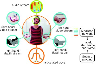
Figure 1: Overview of our method on an example from the 2014 ChaLearn Looking at People (LAP) dataset.

We demonstrate that the proposed scheme can be augmented with more data channels of arbitrary nature by introducing audio into the classification framework.

The major contributions of the present work are the following: We (i) develop a deep learning-based multi-modal and multi-scale framework for gesture detection, localization and recognition, which can be augmented with channels of an arbitrary nature (demonstrated by inclusion of audio); (ii) propose ModDrop for effective fusion of multiple modality channels, which targets learning cross-modality correlations while prohibiting false co-adaptations between data representations and ensuring robustness of the classifier to missing signals; and (iii) introduce an audio-enhanced version of the ChaLearn 2014 LAP dataset.

2 Related work

While having an immediate application in gesture recognition, this work addresses more general aspects of learning representations from raw data and multimodal fusion.

Gesture recognition

Traditional approaches to action and distant gesture recognition from video typically include sparse or dense extraction of spatial or spatio-temporal engineered descriptors followed by classification [15].

Near-range applications may require more accurate reconstruction of hand shapes. A group of recent works is dedicated to inferring the hand pose through pixel-wise hand segmentation and estimating the positions of hand or body joints [16, 17, 18, 19, 20, 21], tracking [22, 23] and graphical models [24, 25].

Multi-modal aspects are of relevance in this domain. In [26], a combination of skeletal features and local occupancy patterns (LOP) were calculated from depth maps to describe hand joints. In [27], skeletal information was integrated in two ways for extracting HoG features from RGB and depth images: either from global bounding boxes containing a whole body or from regions containing an arm, a torso and a head. Similarly, [28, 29, 30] fused skeletal information with HoG features extracted from either RGB or depth, while [31] proposed a combination of a covariance descriptor representing skeletal joint data with spatio-temporal interest points extracted from RGB augmented with audio.

Various multi-layer architectures have been proposed in the context of motion analysis for learning (as opposed to handcrafting) representations directly from data, either in a supervised or unsupervised way. Independent subspace analysis (ISA) [32] as well as autoencoders [33, 9] are examples of efficient unsupervised methods for learning hierarchies of invariant spatio-temporal features. Space-time deep belief networks [34] produce high-level representations of video sequences using convolutional RBMs.

Vanilla supervised convolutional networks have also been explored in this context. A method proposed in [35] is based on low-level preprocessing of the video input and employs a 3D convolutional network for learning of mid-level spatio-temporal representations and classification. Pigou et al. [36] explored this approach in the context of sign language recognition from depth video, while Wu and Chao [37] employed a combination of convnets with HMMs. Recently, Karpathy et al. [10] have proposed a convolutional architecture for large-scale video classification operating at two spatial resolutions (fovea and context streams).

In contrast to existing solutions, in this work we propose a novel specific tree-structured deep learning architecture allowing to classify hand gestures with higher accuracy while restricting the number of free parameters.

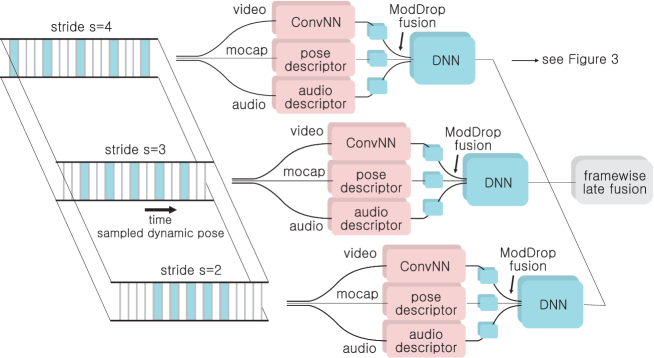
Figure 2: The ModDrop network operating at 3 temporal scales corresponding to 3 durations of dynamic poses.

Multi-modal fusion

While in most practical applications, late fusion of scores output by several models offers a cheap and surprisingly effective solution [7], both late and early fusion of either final or intermediate data representations remain under active investigation.

A significant amount of work on early combining of diverse feature types has been applied to object and action recognition. Multiple Kernel Learning (MKL) [38] has been actively discussed in this context. At the same time, as shown by [39], simple additive or multiplicative averaging of kernels may reach the same level of performance while being orders of magnitude faster.

Ye et al. [40] proposed a late fusion strategy compensating for errors of individual classifiers by minimising the rank of a score matrix. Nataranjan et al. [41] employed multiple strategies, including MKL-based combinations of features, Bayesian model combination, and weighted average fusion of scores from multiple systems.

A number of deep architectures have recently been proposed specifically for multi-modal data. Ngiam et al. [42] employed sparse RBMs and bimodal deep antoencoders to learn cross-modality correlations in the context of audio-visual speech classification of isolated letters and digits. Srivastava et al. [43] used a multi-modal deep Boltzmann machine in a generative fashion to tackle the problem of integrating images and text annotations. Kahou et al. [7] won the 2013 Emotion Recognition in the Wild Challenge by training convolutional architectures on several modalities, such as facial expressions from video, audio, scene context and features extracted around mouth regions. Wu et al. [44] paid special attention to exploring inter-feature and inter-class relationships in deep neural networks for video analysis. Finally, in [45] the authors proposed a multi-modal convolutional network for gesture detection and classification from a combination of depth, skeletal information and audio.

In this work, we explore multimodal deep learning in more detail and pay special attention to encorporating the specifics of multimodality in the training procedure.

3 Gesture classification

On a dataset such as ChaLearn 2014 LAP, we face several key challenges: learning representations at multiple spatial and temporal scales, integrating the various modalities, and training a complex model when the number of labeled examples is not at web-scale like static image datasets (e.g. [3]). We start by describing how the first two challenges are overcome at an architectural level. Our training strategy addressing the last issue is described in Sec. 4.

Our proposed multi-scale deep neural network consists of a combination of single-scale paths connected in parallel (see Fig. 2). Each path independently learns a representation and performs gesture classification at its own temporal scale given input from RGBD video and pose signals (an audio channel can be also added, if available). Predictions from all paths are aggregated through additive late fusion.

To differentiate among temporal scales, a notion of dynamic pose is introduced, meaning a sequence of video frames, synchronized across modalities, sampled with a given temporal stride $s$ and concatenated to form a spatio-temporal 3D volume (similar to earlier works, such as [46]). Varying the value of $s$ allows the model to leverage multiple temporal scales for prediction, accommodating differences in tempos and styles of articulation. Our model is therefore different from the one proposed in [4], where by “multi-scale” Farabet et al. imply a multi-resolution spatial pyramid rather than a fusion of temporal sampling strategies. Regardless of the stride $s$, we use the same number of frames (5) at each scale. Fig. 2 shows the paths used in this work. At each scale and for each dynamic pose, the classifier outputs a per-class score.

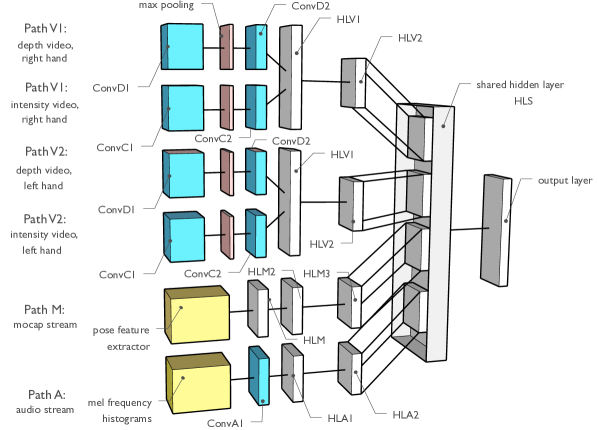
Figure 3: Single-scale deep architecture. Individual classifiers are pre-trained for each data modality (paths V1, V2, M, A) and then fused using a 2-layer fully connected network initialized in a specific way (see Sec. 4).

All available modalities, such as depth, gray scale video, articulated pose, and eventually audio, contribute to the network’s prediction. Global appearance of each gesture instance is captured by the skeleton descriptor, while video streams convey additional information about hand shapes and their dynamics which are crucial for discriminating between gesture classes performed in similar body poses.

Due to the high dimensionality of the data and the non-linear nature of cross-modality structure, an immediate concatenation of raw skeleton and video signals is sub-optimal. However, initial discriminative learning of individual data representations from each isolated channel followed by fusion has proven to be efficient in similar tasks [42]. Therefore, we first learn discriminative data representations within each separate channel, followed by joint fine tuning and fusion by a meta-classifier independently at each scale. More details are given in Sec. 4. A shared set of hidden layers is employed at different levels for, first, fusing of “similar by nature” gray scale and depth video streams and, second, combining the obtained joint video representation with the transformed articulated pose descriptor (and audio signal, if available).

3.1 Articulated pose

The full body skeleton provided by modern consumer depth cameras and associated middleware consists of 20 or fewer joints identified by their coordinates in a 3D coordinate system aligned with the depth sensor. For our purposes we exploit only 11 joints corresponding to the upper body: Head, Shoulder and Hips central points, as well as left and right Hip, Shoulder, Elbow and Hand joints.

We formulate a pose descriptor consisting of 7 logical subsets as described in [47]. Following [48], we first calculate normalized joint positions, as well as their velocities and accelerations, and then augment the descriptor with a set of characteristic angles and pairwise distances.

The skeleton is represented as a tree structure with the HipCenter joint playing the role of a root node. Its coordinates are subtracted from the rest of the vectors to eliminate the influence of position of the body in space. To compensate for differences in body sizes, proportions and shapes, we start from the top of the tree and iteratively normalize each skeleton segment to a corresponding average “bone” length estimated from all available training data. Once the normalized joint positions are obtained, we perform Gaussian smoothing along the temporal dimension ($\sigma{=}1$, filter $5{\times}1$) to decrease the influence of skeleton jitter.

Joint velocities and joint accelerations are calculated as first and second derivatives of normalized joint positions.

Inclination angles are formed by all triples of anatomically connected joints plus two “virtual” angles [47].

Azimuth angles provide additional information about the pose in the coordinate space associated with the body. We apply PCA on the positions of 6 torso joints. Then for each pair of connected bones, we calculate angles between projections of the second bone and the vector on the plane perpendicular to the orientation of the first bone.

Bending angles are a set of angles between a basis vector, perpendicular to the torso, and joint positions.

Finally, we include pairwise distances between all normalized joint positions.

Combined together, this produces a 183-dimensional pose descriptor for each video frame. Finally, each feature is normalized to zero mean and unit variance.

A set of consequent 5 frame descriptors sampled with a given stride $s$ are concatenated to form a $915$-dimensional dynamic pose descriptor which is further used for gesture classification. The two subsets of features involving derivatives contain dynamic information and for dense sampling may be partially redundant as several occurrences of the same frame are stacked when a dynamic pose descriptor is formulated. Although theoretically unnecessary, this is beneficial when the amount of training data is limited.

3.2 Depth and intensity video

Two video streams serve as a source of information about hand pose and finger articulation. Bounding boxes containing images of hands are cropped around positions of the RightHand and LeftHand joints. To eliminate the influence of the person’s position with respect to the camera and keep the hand size approximately constant, the size of each bounding box is normalized by the distance between the hand and the sensor.

Within each set of frames forming a dynamic pose, hand position is stabilized by minimizing inter-frame square-root distances calculated as a sum over all pixels, and corresponding frames are concatenated to form a single spatio-temporal volume. The color stream is converted to gray scale, and both depth and intensity frames are normalized to zero mean and unit variance. Left hand videos are flipped about the vertical axis and combined with right hand instances in a single training set.

During modality-wise pre-training, video pathways are adapted to produce predictions for each hand, rather than for the whole gesture. Therefore, we introduce an additional step to eliminate possible noise associated with switching from one active hand to another. For one-handed gesture classes, we detect the active hand and adjust the class label for the inactive one. In particular, we estimate the motion trajectory length of each hand using the respective joints provided by the skeleton stream (summing lengths of hand trajectories projected to the $x$ and $y$ axes):

$$\Delta=\sum_{t=2}^{5}(|x(t)-x(t-1)|+|y(t)-y(t-1)|),$$ (1)

where $x(t)$ is the x-coordinate of a hand joint (either left or right) and $y(t)$ is its y-coordinate. Finally, the hand with a greater value of $\Delta$ is assigned the label class, while the other hand is assigned the zero-class “no action” label.

For each channel and each hand, we perform 2-stage convolutional learning of data representations independently (first in 3D, then in 2D, see Fig. 3) and fuse the two streams with a set of fully connected hidden layers. Parameters of the convolutional and fully-connected layers at this step are shared between the right hand and left hand pathways. Our experiments have demonstrated that relatively early fusion of depth and intensity features leads to a significant increase in performance, even though the quality of predictions obtained from each channel alone is unsatisfactory.

3.3 Audio stream

Recent advances in the field of speech processing have demonstrated that using weakly preprocessed raw audio data in combination with deep learning leads to higher performance relative to state-of-the-art systems based on hand crafted features (typically from the family of Mel-frequency cepstral coefficients, or MFCC). Deng et al. [49] demonstrated the advantage of using primitive spectral features, such as 2D spectrograms, in combination with deep autoencoders. Ngiam et al. [42] applied the same strategy to the task of multi-modal speech recognition while augmenting the audio signal with visual features. Further experiments from Microsoft [49] have shown that ConvNets appear to be especially efficient in this context since they allow the capture and modeling of structure and invariances that are typical for speech.

Comparative analysis of our previous approach [45] based on phoneme recognition from sequences of MFCC features and a deep learning framework has demonstrated that the latter strategy allows us to obtain significantly better performance on the ChaLearn dataset (see Sec. 7 for more details). Therefore, in this work, the audio signal is processed in the same manner as video data, i.e. by feature learning within a convolutional architecture.

To preprocess, we perform basic noise filtering and speech detection by thresholding the raw signal along the absolute value of the amplitude ($\tau_{1}$). Short, isolated peaks of duration less than $\tau_{2}$ are also ignored during training. We apply a short-time Fourier transform on the raw audio signal to obtain a 2D local spectrogram which is further transformed to the Mel -scale to produce 40 log filter-banks on the frequency range from 133.3 to 6855.5 Hz, i.e. the zero-frequency component is eliminated. In order to synchronize the audio and visual signals, the size of the Hamming window is chosen to correspond to the duration of $L_{1}$ frames with half-frame overlap. A typical output is illustrated in Fig. 4. As it was experimentally demonstrated by [49], the step of the scale transform is important. Even state-of-the-art deep architectures have difficulty learning these kind of non-linear transformations.

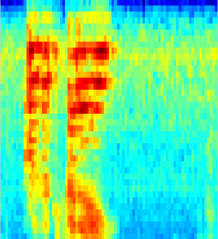
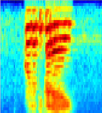
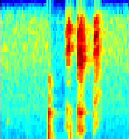
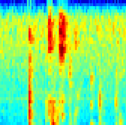
Figure 4: Mel-scaled spectrograms of two pairs of audio samples corresponding to two different gestures.

A one-layer convolutional network in combination with two fully-connected layers form the corresponding path which we, as before, pretrain for preliminary gesture classification from short utterances. The output of the penultimate layer provides audio features for data fusion and modeling temporal dependencies (see Sec. 4).

4 Training procedure

In this section we describe the most important architectural solutions that were critical for our multi-modal setting: per-modality pre-training and aspects of fusion such as the initialization of shared layers. Also, we introduce the concept of multi-modal dropout (ModDrop), which makes the network less sensitive to loss of one or more channels.

Pretraining

Depending on the source and physical nature of a signal, input representation of any modality is characterized by its dimensionality, information density, and associated correlated and uncorrelated noise. Accordingly, a monolithic network taking as an input a combined collection of features from all channels is suboptimal, since a uniform distribution of parameters over the input is likely to overfit one subset of features and underfit the others. Here, performance-based optimization of hyper-parameters may resolve in cumbersome architectures requiring sufficiently larger amounts of training data and computational resources at training and test times. Furthermore, blind fusion of fundamentally different signals at early stages has a high risk of learning false cross-modality correlations and dependencies among them (see Sec. 7). To capture complexity within each channel, separate pretraining of input layers and optimization of hyper parameters for each subtask are required.

Recall Fig. 3 illustrating a single-scale deep multi-modal convolutional network. Initially it starts with six separate pathways: depth and intensity video channels for right (V1) and left (V2) hands, a mocap stream (M) and an audio stream (A). From our observations, inter-modality fusion is effective at early stages if both channels are of the same nature and convey complementary information. On the other hand, mixing modalities which are weakly correlated, is rarely beneficial until the final stage. Accordingly, in our architecture, two video channels corresponding to each hand (layers HLV1 and HLV2) are fused immediately after feature extraction. We postpone any attempt to capture cross-modality correlations of complementary skeleton motion, hand articulation and audio until the shared layer HLS.

Initialization of the fusion process

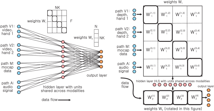
Figure 5: On the left: architecture of shared hidden and output layers. On the right: structure of parameters of shared hidden and output layers (corresponds to the architecture on the left).

Assuming the weights of the modality-specific paths are pre-trained, the next important issue is determining a fusion strategy. Pre-training solves some of the problems related to learning in deep networks with many parameters. However, direct fully-connected wiring of pre-trained paths to the shared layer in large-scale networks is not effective, as the high degrees of freedom afforded by the fusion process may lead to a quick degradation of pre-trained connections. We therefore proceed by initializing the shared layer such that a given hard-wired fusion strategy is performed, and then gradually relax it to more powerful fusion strategies.

A number of works have shown that among fusion strategies, the weighted arithmetic mean of per-model outputs is the least sensitive to errors of individual classifiers [50]. It is often used in practice, outperforming more complex fusion algorithms. Considering the weighted mean as a simple baseline, we aim to initialize the fusion process with this starting point and proceed with gradient descent optimization towards an improved solution.

Unfortunately, implementing the arithmetic mean in the case of early fusion and non-linear shared layers is not straightforward [51]. It has been shown though [52], that in dropout-like [53] systems activation units of complete models produce a weighted normalized geometric mean of per-model outputs. This kind of average approximates the arithmetic mean better than the geometric mean and the quality of this approximation depends on consistency in the neuron activation. We therefore initialize the fusion process to a normalized geometric mean of per-model outputs.

Data fusion is implemented at two different layers: the shared hidden layer (HLS) and the output layer. The weight matrices of these two layers, denoted respectively as $W_{1}$ and $W_{2}$, are block-wise structured and initialized in a specific way, as illustrated in Fig. 5. The left figure shows the architecture in a conventional form as a diagram of connected neurons. The weights of the connections are indicated by matrices. On the right we introduce a less conventional notation, which allows one to better visualize and interpret the block structure. Note that the image scale is chosen for clarity of description and the real aspect ratio between dimensions of $W_{1}$ ($1600{\times}84$) is not preserved, the ratio between vertical sizes of matrix blocks corresponding to different modalities is 9:9:7:7.

We denote the number of hidden units in the modality- specific hidden layers on each path as $F_{k}$, where $k{=}1{\ldots}K$ and $K$ is the number of modality-specific paths. We set the number of units of the shared hidden layer equal to $K{\cdot}N$, where $N$ is the number of target gesture classes.

As a consequence, the matrix $W_{1}$ of the shared hidden layer is of size $F{\times}(N{\cdot}K)$, where $F{=}\sum_{k}F_{k}$, and the weight matrix $W_{2}$ of the output layer is of size $(N{\cdot}K){\times}N$. Weight matrix $W_{1}$ can be thought of as a matrix of $K{\times}K$ blocks, where each block $k$ is of size $F_{k}{\times}N$. This imposes a certain meaning on the units and weights of the network. Each column in a block (and each unit in the shared layer) is therefore related to a specific gesture class. Note that this block structure (and meaning) is forced on the weight matrix during initialization and in the early phases of training. If only the diagonal blocks are non-zero, which is forced at the beginning of the training procedure, then individual modalities are trained independently, and no cross correlations between modalities are captured. During the final phases of training, no structure is imposed and the weights can evolve freely. Formally, the activation of each hidden unit $h_{l}^{k}$ in the shared layer can be expressed as:

$$h_{l}^{(k)}\!\!=\!\sigma\!\left[\!\vphantom{\sum}\right.\sum_{i=1}^{F_{k}}\!w_{i,l}^{(k,k)}\!x_{i}^{(k)}\!\!+\!\gamma\!\!\sum_{\begin{subarray}{c}m=1\\ m\neq k\end{subarray}}^{K}\!\sum_{i=1}^{F_{n}}\!w_{i,l}^{(m,k)}x_{i}^{(m)}\!\!+b_{l}^{(k)}\!\left.\vphantom{\sum}\right]$$ (2)

where $h_{l}^{(k)}$ is unit $l$ initially related to modality $k$, and all $w$ are from weight matrix $W_{1}$. Notation $w_{i,l}^{(m,k)}$ stands for a weight between non-shared hidden unit $i$ from the output layer of modality channel $m$ and the given shared hidden unit $l$ related to modality $k$. Accordingly, $x_{i}^{(m)}$ is input number $i$ from channel $m$, $\sigma$ is an activation function. Finally, $b_{l}^{(k)}$ is a bias of the shared hidden unit $h_{l}^{(k)}$. The first term contains the diagonal blocks and the second term contains the off-diagonal weights. Setting $\gamma{=}0$ freezes learning of the off-diagonal weights responsible for inter-modality correlations.

This initial meaning forced onto both weight matrices $W_{1}$ and $W_{2}$ produces a setting where the hidden layer is organized into $K$ subsets of units $h_{l}^{(k)}$, one for each modality $k$, and where each subset comprises $N$ units, one for each gesture class. The weight matrix $W_{2}$ is initialized in a way such that these units are interpreted as posterior probabilities for gesture classes, which are averaged over modalities by the output layer controlled by weight matrix $W_{2}$. In particular, each of the $N{\times}N$ blocks of the matrix $W_{2}$ (denoted as $v^{(k)}$) is initialized as an identity matrix, which results in the following expression for the output units, which are softmax activated:

$$o_{j}=\dfrac{e^{\sum_{k=1}^{K}\sum_{c=1}^{N}v^{(k)}_{j,c}h^{(k)}_{c}}}{\sum_{i=1}^{N}e^{\sum_{k=1}^{K}\sum_{c=1}^{N}v^{(k)}_{i,c}h^{(k)}_{c}}}=\dfrac{e^{\sum_{k=1}^{K}h^{(k)}_{j}}}{\sum_{i=1}^{N}e^{\sum_{k=1}^{K}h^{(k)}_{i}}}$$ (3)

where we used that $v_{j,c}^{(k)}{=}1/K\textrm{ if }j{=}c$ and $0$ else.

From (3) we can see that the diagonal initialization of $W_{2}$ forces the output layer to perform modality fusion as a normalized geometric mean over modalities, as motivated in the initial part of this section. Again, this setting is forced in the early stages of training and relaxed later, freeing the output layer to more complex fusion strategies.

ModDrop: multimodal dropout

Inspired by the concept of dropout [53] as the normalized geometric mean of an exponential number of weakly trained models, we aim on exploiting a priori information about groupings in the feature set. We initiate a similar process but with a fixed number of models corresponding to separate modalities and pre-trained to convergence. We have two main motivations: (i) to learn a shared model while preserving uniqueness of per-channel features and avoiding false co-adaptations between modalities; (ii) to handle missing data in one or more of the channels at test time. The key idea is to train the shared model in a way that it would be capable of producing meaningful predictions from an arbitrary number of available modalities (with an expected loss in precision when some signals are missing).

Formally, let us consider a set of $\mathcal{M}^{(k)}$, $k{=}1{\ldots}K$ modality-specific models. During pretraining, the joint learning objective can be generally formulated as follows:

$$\mathcal{L}_{\mathrm{pretraining}}=\sum_{k=1}^{K}\mathcal{L}\left[\mathcal{M}^{(k)}\right]+\alpha\sum_{h=1}^{H}||W_{h}||^{2},$$ (4)

where each term in the first sum represents a loss of the corresponding modality-specific model (in our case, negative log likelihood, summarized over all samples $x_{d}$ for the given modality $k$ from the training set $|\mathcal{D}|$):

$$\mathcal{L}\left[\mathcal{M}^{(k)}\right]=-\sum_{d\in\mathcal{D}}\log{o^{(k)}_{Y}(Y=y_{d}|x_{d}^{(k)})},$$ (5)

where $o^{(k)}_{Y}$ is output probability distribution over classes of the network corresponding to modality $k$ and $y_{d}$ is a ground truth label for a given sample $d$.

The second term in Eq. 4 is $L_{2}$ regularization on all weights $W_{h}$ from all hidden layers $h{=}1{\ldots}H$ in the network (with weight $\alpha$). At this pretraining stage, all loss terms in the first sum are minimized independently.

Once the weight matrices $W_{1}$ and $W_{2}$ are initialized with pre-trained diagonal elements and initially zeroed out off-diagonal blocks of weights are relaxed (i.e. $\gamma{=}1$ in Eq. 2), fusion is learned from the training data. The desired training objective during the fusion process can be formulated as a combination of losses of all possible combinations of modality-specific models:

$$\!\!\!\mathcal{L}_{\Sigma} \!=\!\!\sum_{k=1}^{K}\!\mathcal{L}\!\left[\!\mathcal{M}^{(k)}\!\right]\!+\!\!\!\sum_{k\neq m}\!\!\mathcal{L}\!\left[\!\mathcal{M}^{(k,m)}\!\right]\!+\!\!\!\!\!\!\sum_{k\neq m\neq n}\!\!\!\!\!\mathcal{L}\!\left[\!\mathcal{M}^{(k,m,n)}\!\right]\!+\!{\ldots}\vspace*{-35pt}$$

$$+\alpha\sum_{h=1}^{H}\!||W_{h}||^{2}\!=\!\sum_{S\in\mathcal{P}({\mathcal{M}}^{(k)})}\!\!\!\mathcal{L}\left[S\right]+\alpha\sum_{h=1}^{H}||W_{h}||^{2},$$ (6)

where $\mathcal{M}^{(k,m)}$ indicates fusion of models $\mathcal{M}^{(k)}$, $\mathcal{P}(\mathcal{M}^{(k)})$ is the powerset of all models, whose size is $2^{K}$, and $S$ is an element of the power set corresponding to all possible combinations of modalities.

The loss function formulated in (4) reflects the objective of the training procedure, but in practice we approximate this objective by ModDrop as iterative interchangeable training of one term at a time. In particular, the fusion process starts by joint training through backpropagation over the shared layers and fine tuning all modality specific paths. As this step, the network takes as an input multi-modal training samples $\{\delta^{(k)}x_{d}^{(k)}\}$, $k=1{\ldots}K$ from the training set $|\mathcal{D}|$, where for each sample each modality component $x_{d}^{(k)}$ is dropped (set to $0$) with a certain probability $q^{(k)}{=}1{-}p^{(k)}$ indicated by Bernoulli selector $\delta^{(k)}{:}\,P(\delta^{(k)}{=}1){=}p^{(k)}$. Accordingly, one step of gradient descent given an input with a certain number of non-zero modality components minimizes the loss of a corresponding multi-modal subnetwork denoted as $\{\delta^{(k)}\mathcal{M}^{(k)}\}$. This aligns well with the initialization process described above, which ensures that modality-specific subnetworks that are being removed or added by ModDrop are well pre-trained in advance.

Regularization properties

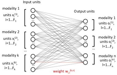
Figure 6: Toy network architecture and notations used for derivation of ModDrop regularization properties.

In the following we will study the regularization properties of modality-wise dropout on inputs (ModDrop) on a simpler network architecture, namely a one-layer shared network with $K$ modality specific paths and sigmoid activation units. Input $i$ for modality $k$ is denoted as $x_{i}^{(k)}$ and we assume that there are $F_{k}$ inputs coming from each modality $k$ (see Fig. 6). Output unit $l$ related to modality $n$ is denoted as $o_{l}^{(n)}$. Finally, a weight coefficient connecting input unit $x_{i}^{(k)}$ with output unit $o_{l}^{(n)}$ is denoted as $w_{i,l}^{(k,n)}$.

In our example, output units are sigmoidal, i.e. for each output unit $o_{l}$ related to modality $n$, $o_{l}^{(n)}=\sigma(s_{l}^{(n)})=1/(1+e^{-\lambda{s_{l}^{(n)}}})$, where $s_{l}^{(n)}{=}\sum_{k=1}^{K}\sum_{i}^{F_{k}}w_{i,l}^{(k,n)}x_{i}^{(k)}$ is the input to the activation function coming to the given output unit from the previous layer, and $\lambda$ is a coefficient.

We minimize cross-entropy error calculated from the targets $y$ (indices are dropped for simplicity)

$$E=-(y\log{o}+(1-y)\log{(1-o)}),$$ (7)

whose partial derivatives can be given as follows:

$$\dfrac{\partial E}{\partial w}=\dfrac{\partial E}{\partial o}\dfrac{\partial o}{\partial s}\dfrac{\partial s}{\partial w},\quad\dfrac{\partial E}{\partial o}=-y\dfrac{1}{o}+(1-o)\dfrac{1}{1-o},$$

$$\dfrac{\partial o}{\partial s}=\lambda o(1-o),\quad\dfrac{\partial E}{\partial w}=-\lambda(y-o)\dfrac{\partial s}{\partial w}.$$ (8)

Along the lines of [52], we consider two situations corresponding to two different loss functions: $E_{\Sigma}$, corresponding to the “complete network” where all modalities are present, and $\tilde{E}$ where ModDrop is performed. In our case, we assume that whole modalities (sets of units corresponding to a given modality $k$) are either dropped or preserved. In a ModDrop network, this can be formulated such that the input to the activation function of a given output unit $l$ related to modality $n$ (denoted as $\tilde{s}_{l}^{(n)}$) involves a Bernoulli selector variable $\delta^{(k)}$ for each modality $k$ which can take on values in $\{0,1\}$ and is activated with probablity $p^{(k)}$:

$$\tilde{s}_{l}^{(n)}=\sum_{k=1}^{K}\delta^{(k)}\sum_{i=1}^{F_{k}}w_{i,l}^{(k,n)}x_{i}^{(k)}$$ (9)

As a reminder, in the case of the complete network (all channels are present) the output activation it the following:

$$s_{l}^{(n)}=\sum_{k=1}^{K}\sum_{i=1}^{F_{k}}w_{i,l}^{(k,n)}x_{i}^{(k)}$$ (10)

As the following reasoning always concerns a single output unit $l$ related to modality $n$, from now on these indices will be dropped for simplicity of notation. Therefore, we denote $s=s_{l}^{(n)}$, $\tilde{s}=\tilde{s}_{l}^{(n)}$ and $w_{i}^{(k)}=w_{i,l}^{(k,n)}$.

Gradients of corresponding complete and ModDrop sums with respect to weights can be expressed as follows:

$$\dfrac{\partial\tilde{s}}{\partial w_{i}^{(k)}}=\delta^{(k)}x_{i}^{(k)},\quad\dfrac{\partial s}{\partial w_{i}^{(k)}}=x_{i}^{(k)}$$ (11)

Using the gradient of the error $E$

$$\dfrac{\partial E}{\partial w_{i}^{(k)}}=-\lambda\left[y-\sigma(s)\right]\dfrac{\partial s}{\partial w_{i}^{(k)}},$$ (12)

the gradient of the error for the complete network is:

$$\dfrac{\partial E_{\Sigma}}{\partial w_{i}^{(k)}}=-\lambda x_{i}^{(k)}\!\left[y\vphantom{\sum}\right.-\sigma{\left(\vphantom{\sum}\right.\sum_{m=1}^{K}\sum_{j=1}^{F_{m}}w_{j}^{(m)}x_{j}^{(m)}\left.\!\vphantom{\sum}\right)}\left.\!\!\vphantom{\sum}\right]$$ (13)

In the case of ModDrop, for one realization of the network where a modality is dropped with corresponding probability $q^{(k)}{=}1{-}p^{(k)}$, indicated by the means of Bernoulli selectors $\delta^{(k)}$, i.e. $P(\delta^{(k)}{=}1){=}p^{(k)}$, we get:

$$\!\dfrac{\partial\tilde{E}}{\partial w_{i}^{(k)}}\!=\!-\lambda\delta^{(k)}\!x_{i}^{(k)}\!\left[\vphantom{\sum}\right.\!y-\sigma{\left(\!\vphantom{\sum}\right.\sum_{m=1}^{K}\!\!\delta^{(m)}\!\sum_{j=1}^{F_{m}}w_{j}^{(m)}\!x_{j}^{(m)}\!\left.\vphantom{\sum}\right)}\!\!\left.\vphantom{\sum}\right]\!\!\!\!$$ (14)

Taking the expectation of this expression requires an expression introduced in [52], which approximates $E[\sigma(x)]$ by $\sigma(E[x])$. We take the expectation over the $\delta^{(m)}$ with the exception of $\delta^{(k)}{=}1$, which is the Bernouilli selector of the modality $k$ for which the derivative is calculated:

$$E\left[\!\vphantom{\tilde{\sum}}\right.\dfrac{\partial\tilde{E}}{\partial w_{i}^{(k)}}\left.\vphantom{\tilde{\sum}}\!\!\right] \!\approx\!-\lambda p^{(k)}\!x_{i}^{(k)}\!\left[y\vphantom{\sum}\right.-\sigma\!\left(\!\vphantom{\sum}\right.\sum_{m\neq k}^{K}p^{(m)}\!\sum_{j=1}^{F_{m}}w_{j}^{(m)}\!x_{j}^{(m)}$$

$$+\!\sum_{j=1}^{F_{k}}\!w_{j}^{(k)}\!x_{j}^{(k)}\!\left.\vphantom{\sum}\right)\!\left.\vphantom{\sum}\right]\!=\!-\lambda p^{(k)}x_{i}^{(k)}\left[y\vphantom{\sum}\right.\!-\!\sigma\!\left(\vphantom{\sum}\!\right.\sum_{m\neq k}^{K}\sum_{j=1}^{F_{m}}w_{j}^{(m)}\!x_{j}^{(m)}$$

$$-\!\!\sum_{m\neq k}^{K}\!(1\!-\!p^{(m)})\!\sum_{j=1}^{F_{m}}w_{j}^{(m)}\!x_{j}^{(m)}\!\!+\!\!\sum_{j=1}^{F_{k}}w_{j}^{(k)}\!x_{j}^{(k)}\!\!\left.\vphantom{\sum}\right)\!\!\left.\vphantom{\sum}\right]\!\!=\!-\lambda p^{(k)}\!x_{i}^{(k)}$$

$$\times\!\!\left[y\vphantom{\sum}\right.\!-\!\sigma\!\left(\!\vphantom{\sum}\right.\!\sum_{m=1}^{K}\!\sum_{j=1}^{F_{m}}w_{j}^{(m)}\!x_{j}^{(m)}\!\!\!-\!\!\sum_{m\neq k}^{K}\!(1\!-\!p^{(m)})\!\sum_{j=1}^{F_{m}}w_{j}^{(m)}\!x_{j}^{(m)}\!\left.\vphantom{\sum}\right)\!\!\left.\vphantom{\sum}\right]$$

Taking the first-order Taylor expansion of the activation function $\sigma$ around $s=\sum_{m}\sum_{j}w_{j}^{(m)}\!x_{j}^{(m)}$ gives

$$\centering\!E\!\!\left[\!\vphantom{\tilde{\sum}}\right.\!\dfrac{\partial\tilde{E}}{\partial w_{i}^{(k)}}\!\left.\!\vphantom{\tilde{\sum}}\!\right]\!\!\@add@centering \approx\!\!-\lambda p^{(k)}\!x_{i}^{(k)}\!\!\left[\!\vphantom{\sum}\right.\!y\!-\!\sigma_{s}\!\!+\!\sigma_{s}^{\prime}\!\!\sum_{m\neq k}^{K}\!\!(1\!-\!p^{(m)}\!)\!\!\sum_{j=1}^{F_{m}}\!\!w_{j}^{(m)}\!x_{j}^{(m)}\left.\vphantom{\sum}\!\!\right]$$

where $\sigma^{\prime}_{s}\!{=}\sigma^{\prime}(s)\!{=}\sigma(s)\!{/}\!(1{-}\sigma(s))$. Substituting equation (13),

$$\!\!E\!\!\left[\!\vphantom{\tilde{\sum}}\right.\!\dfrac{\partial\tilde{E}}{\partial w_{i}^{(k)}}\!\left.\vphantom{\tilde{\sum}}\!\!\right]\!\!\approx\!p^{(k)}\!\!\dfrac{\partial E_{\Sigma}}{\partial w_{i}^{(k)}}\!-\!\lambda\sigma_{\!\!s}^{\prime}\!x_{i}^{(k)}\!p^{(k)}\!\!\!\sum_{m\neq k}^{K}\!\!(1\!-\!p^{(m)}\!)\!\!\sum_{j=1}^{F_{k}}\!w_{j}^{(m)}\!x_{j}^{(m)}$$

If $p^{(k)}{=}p^{(m)}{=}p$ then $p(1{-}p){=}\textrm{Var}(\delta)$. From the gradient, we can calculate the error $\tilde{E}$ integrating out the partial derivatives and summing over the weights $i$:

$$\!\!\tilde{E}\!\approx\!pE_{\Sigma}\!-\!\!\lambda\sigma_{\!\!s}^{\prime}\textrm{Var}(\delta)\!\!\sum_{k=1}^{K}\!\sum_{m\neq k}^{K}\!\sum_{i{=}1}^{F_{k}}\!\sum_{j=1}^{F_{m}}\!\!w_{i}^{(k)}\!w_{j}^{(m)}\!x_{i}^{(k)}\!x_{j}^{(m)}$$ (15)

As it can be seen, the error of the network with ModDrop is approximately equal to the error of the complete model (up to a coefficient) minus an additional term including a sum of products of inputs and weights corresponding to different modalities in all possible combinations. We need to stress here that this second term reflects exclusively cross-modality correlations and does not involve multiplications of inputs from the same channel. To understand what influence the cross-product term has on the training process, we analyse two extreme cases depending on whether or not signals in different channels are correlated.

Let us consider two input units $x_{i}^{(k)}$ and $x_{j}^{(m)}$ coming from different modalities and first assume that they are independent and therefore uncorrelated. Since each network input is normalized to zero mean, the expectation is also equal to zero:

$$E\!\left[\!\!\vphantom{\tilde{x}}\,\right.x_{i}^{(k)}\!x_{j}^{(m)}\left.\vphantom{\tilde{x}}\!\!\right]{=}E\!\left[\!\vphantom{\tilde{x}}\right.x_{i}^{(k)}\left.\vphantom{\tilde{x}}\!\!\right]\!E\!\left[\vphantom{\tilde{x}}\,\right.\!\!x_{j}^{(m)}\left.\vphantom{\tilde{x}}\!\!\right]{=}0.$$ (16)

Weights in a single layer of a neural network typically obey a unimodal distribution with zero expectation [54]. It can be shown [55] that under these assumptions, Lyapunov’s condition is satisfied and that Lyapunov’s central mean theorem holds; in this case the sum of products of inputs and weights will tend to a normal distribution given that the number of training samples is sufficiently large. As both the input and weight distributions have zero mean, the resulting law is also centralized and its variance is defined by the magnitudes of the weights (assuming inputs are fixed).

We conclude that, assuming independence of inputs in different channels, the second term in equation (15) tends to vanish if the number of training samples in a batch is sufficiently large. In practice, additional regularization on weights is required to prevent weights from exploding.

Now let us consider a more interesting scenario when two inputs $x_{i}^{(k)}$ and $x_{j}^{(m)}$ belonging to different modalities are positively correlated. In this case, given zero mean distributions on each input, their product is expected to be positive:

$$E\!\left[\!\!\vphantom{\tilde{x}}\,\right.x_{i}^{(k)}\!x_{j}^{(m)}\left.\vphantom{\tilde{x}}\!\!\right]{=}E\!\left[\!\vphantom{\tilde{x}}\right.x_{i}^{(k)}\left.\vphantom{\tilde{x}}\!\!\right]\!E\!\left[\vphantom{\tilde{x}}\,\right.\!\!x_{j}^{(m)}\left.\vphantom{\tilde{x}}\!\!\right]+\text{Cov}\!\left[\!\vphantom{\tilde{x}}\right.x_{i}^{(k)}\!\!,x_{j}^{(k)}\left.\vphantom{\tilde{x}}\!\right]\!.$$ (17)

Therefore, on each step of gradient descent this term enforces the product $w_{i}^{(k)}w_{j}^{(m)}$ to be positive and therefore introduces correlations between these weights (given, again, the additional regularization term preventing one of the multipliers from growing significantly faster than the other). The same logic applies if inputs are negatively correlated, which would enforce negative correlations on corresponding weights. Accordingly, for correlated modalities this additional term in the error function introduced by ModDrop acts as a cross-modality regularizer forcing the network to generalize by discovering similarities between different signals and “aligning” them with each other by introducing soft ties on the corresponding weights.

Finally, as has been shown by [52] for dropout, the multiplier proportional to the derivative of the sigmoid activation makes the regularization effect adaptive to the magnitude of the weights. As a result, it is strong in the mid-range of weights, plays a less significant role when weights are small and gradually weakens with saturation.

Our experiments have shown that ModDrop achieves the best results if combined with dropout, which introduces an adaptive L2 regularization term $\hat{E}$ in the error function [52]:

$$\hat{E}\approx\lambda\sigma_{s}^{\prime}\text{Var}(\hat{\delta})\sum_{k=1}^{K}\sum_{i=1}^{F_{k}}\left[w_{i}^{(k)}x_{i}^{(k)}\right]^{2}\!\!\!,$$ (18)

where $\hat{\delta}$ is a Bernoulli selector variable, $P(\hat{\delta}{=}1){=}\hat{p}$ and $\hat{p}$ is the probability that a given input unit is present.

5 Inter-scale fusion during test time

Once individual single-scale predictions are obtained, we employ a simple voting strategy for fusion with a single weight per model. We note here that introducing additional per-class per-model weights and training meta-classifiers (such as an MLP) on this step quickly leads to overfitting.

At each given frame $t$, per-class network outputs $o_{k}$ are obtained via per-frame aggregation and temporal filtering of predictions at each scale with corresponding weights $\mu_{s}$ defined empirically:

$$o_{k}(t)=\sum_{s=2}^{4}\mu_{s}\sum_{j=-4s}^{0}o_{s,k}(t+j),$$ (19)

where $o_{s,k}(t+j)$ is the score of class $k$ obtained for a spatio-temporal block sampled starting from the frame $t+j$ at step $s$. Finally, the frame is assigned the class label $l(t)$ having the maximum score: $l(t)=\operatorname*{argmax}_{k}{o_{k}(t)}$.

6 Gesture localization

With increasing duration of a dynamic pose, recognition rates of the classifier increase at a cost of loss in precision in gesture localization. Using wider sliding windows leads to noisy predictions at pre-stroke and post-stroke phases due to the overlap of several gesture instances at once. On the other hand, too short dynamic poses are not discriminative either, as most gesture classes at their initial and final stages have a similar appearance (e.g. raising or lowering hands).

There exists vast literature on temporal video segmentation ([56]), however in this work we employ a simpler and yet efficient solution. To address this issue, we introduce an additional binary classifier to distinguish resting moments from periods of activity. Trained on dynamic poses at the finest temporal resolution $s{=}1$, this classifier is able to precisely localize starting and ending points of each gesture.

The module is a two-layer fully connected network taking as an input the articulated pose descriptor. All training frames having a gesture label are used as positive examples, while a set of frames right before and after such gesture are considered as negatives. Each frame is thus assigned with a label “motion” or “no motion” with accuracy of $98\%$.

To combine the classification and localization modules, frame-wise gesture class predictions are first obtained as described in Section 5. Output predictions at the beginning and at the end of each gesture are typically noisy. Therefore, for each spotted gesture, its boundaries are extended or shrunk towards the closest switching point produced by the binary classifier (assuming that this point is in a vicinity of the initially detected boundary).

7 Experiments

The Chalearn 2014 Looking at People Challenge (track 3) dataset [14] consists of 13,858 instances of Italian conversational gestures performed by different people and recorded with a consumer RGB-D sensor. It includes color, depth video and mocap streams. The gestures are drawn from a large vocabulary, from which 20 categories are identified to detect and recognize and the rest are considered as arbitrary movements. Each gesture in the training set is accompanied by a ground truth label as well as information about its start- and end-points. For the challenge, the corpus was split into development, validation and test sets. The test data was released to participants after submitting their source code.

To further explore the dynamics of learning in multi-modal systems, we augmented the data with audio recordings extracted from a dataset released under the framework of the Chalearn 2013 Multi-modal Challenge on Gesture Recognition [57]. Differences between the 2014 and 2013 versions are mainly permutations in sequence ordering, improved quality of gesture annotations, and a different metric used for evaluation: the Jaccard index in 2014 instead of the Levenshtein distance in 2013. As a result, each gesture in a video sequence is accompanied by a corresponding vocal phrase bearing the same meaning. Due to dialectical and personal differences in pronunciation and vocabulary, gesture recognition from the audio channel alone was surprisingly challenging.

To summarize, we report results for two settings: i) the original dataset used for the ChaLearn 2014 Looking at People (LAP) Challenge (track 3), ii) an extended version of the dataset augmented with audio recordings taken from the Chalearn 2013 Multi-modal Gesture Recognition dataset.

7.1 Experimental setup

Hyper-parameters of the multi-modal neural network for classification are provided in Table I. The architecture is identical for each temporal scale. Gesture localization is performed with another MLP with 300 hidden units (see Section 6). All hidden units in the classification and localization modules have hyperbolic tangent activations. Hyper-parameters were optimized on the validation data with early stopping to prevent the models from overfitting and without additional regularization. For simplicity, fusion weights for the different temporal scales are set to $\mu_{s}{=}1$, as well as the weight of the baseline model (see Section 5). The deep learning architecture is implemented with the Theano library [58]. A single-scale predictor operates at frame rates close to real time (24 fps on GPU).

Path	Layer	Filter size / # units	# parameters	Pooling
Paths V1, V2	Input D1,D2	$72{\times}72{\times}5$	-	$2{\times}2{\times}1$
	ConvD1	$25{\times}5{\times}5{\times}3$	1900	$2{\times}2{\times}3$
	ConvD2	$25{\times}5{\times}5$	650	$1{\times}1$
	Input C1,C2	$72{\times}72{\times}5$	-	$2{\times}2{\times}1$
	ConvC1	$25{\times}5{\times}5{\times}3$	1900	$2{\times}2{\times}3$
	ConvC2	$25{\times}5{\times}5$	650	$1{\times}1$
	HLV1	$900$	3 240 900	-
	HLV2	$450$	405 450	-
Path M	Input M	$183$	-
	HLM1	$700$	128 800	-
	HLM2	$700$	490 700	-
	HLM3	$350$	245 350	-
Path A	Input A	$40{\times}9$	-	$1{\times 1}$
	ConvA1	$25{\times}5{\times}5$	650	$1{\times}1$
	HLA1	$700$	3 150 000	-
	HLA2	$350$	245 350	-
Shared	HLS1	$1600$	3 681 600	-
	HLS2	$84$	134 484	-
	Output layer	$21$	1785	-

TABLE I: Hyper-parameters (for a single temporal scale)

We followed the evaluation procedure proposed by the challenge organizers and adopted the Jaccard Index to quantify model performance:

$$J_{s,n}=\dfrac{A_{s,n}\cap B_{s,n}}{A_{s,n}\cup B_{s,n}},$$ (20)

where $A_{s,n}$ is the ground truth label of gesture $n$ in sequence $s$, and $B_{s,n}$ is the obtained prediction for the given gesture class in the same sequence. Here $A_{s,n}$ and $B_{s,n}$ are binary vectors where the frames in which the given gesture is being performed are marked with 1 and the rest with 0. Overall performance was calculated as the mean Jaccard index among all gesture categories and all sequences, with equal weight for all gesture classes.

7.2 Baseline models

In addition to the main pipeline, we have implemented a baseline model based on an ensemble classifier trained in a similar iterative fashion but on purely handcrafted descriptors. The purpose of this comparison was to explore relative advantages and disadvantages of using learned representations as well as the nuances of fusion. We also found it beneficial to combine the proposed deep network with the baseline method in a hybrid model (see Table V).

The baseline used for visual models is described in detail in [47]. We use depth and intensity hand images and extract three sets of features. HoG features describe the hand pose in the image plane. Histograms of depths describe pose along the third spatial dimension. The third set of features is comprised of derivatives of HOGs and depth histograms, which reflect temporal dynamics of hand shape.

Extremely randomized trees (ERT) [59] are adopted for data fusion and gesture classification. During training, we followed the same iterative strategy as in the case of the neural architecture (see [47] for more details).

A baseline has also been created for the audio channel, where we compare the proposed deep learning approach to a traditional phoneme recognition framework, as described in [45], and implemented with the Julius engine [60]. In this approach, each gesture is associated with a pre-defined vocabulary of possible ordered sequences of phonemes that can correspond to a single word or a phrase. After spotting and segmenting periods of voice activity, each utterance is assigned a n-best list of gesture classes with corresponding scores. Finally, frequencies of appearances of each gesture class in the list are treated as output class probabilities.

7.3 Results on the ChaLearn 2014 LAP dataset

#	Team	Score	#	Team	Score
$\mathbf{1}$	Ours [47]	$\mathbf{0.850}$	$7$	Camgoz et al. [61]	$0.747$
$2$	​Monnier​ et​ al.​ [29]​	$0.834$	$8$	​Evangelidis​ et​ al. [62]​	$0.745$
$3$	Chang [30]	$0.827$	$9$	​Undisclosed authors​	$0.689$
$4$	Peng et al. [63]	$0.792$	$10$	Chen et al. [64]	$0.649$
$5$	Pigou et al. [36]	$0.789$	$\ldots$
$6$	Wu [37]	$0.787$	$17$	Undisclosed authors	$0.271$
Ours, improved results after the competition $\mathbf{0.870}$

TABLE II: Official ChaLearn 2014 LAP Challenge (track 3) results, visual modalities only.

Step	Pose	Video	Pose & Video	Audio	All
$2$	$0.823$	$0.818$	$0.856$	$0.709$	$0.870$
$3$	$0.824$	$0.817$	$0.859$	$0.731$	$0.873$
$4$	$0.827$	$0.825$	$0.859$	$0.714$	$0.880$
all	${0.831}$	${0.836}$	0.868	0.734	0.881

TABLE III: Post-competition performance at different temporal scales with gesture localization (Jaccard index).

The top 10 scores of the ChaLearn 2014 LAP Challenge (track 3) are reported in Table II. Our winning entry [47] corresponding to a hybrid model (i.e. a combination of the proposed deep neural architecture and the ERT baseline model) surpasses the second best score by a margin of 1.61 percentage points. We also note that the multi-scale neural architecture still achieves the best performance, as well as the top one-scale neural model alone (see Tables III and V). In post-challenge work we were able to further improve the score by 2.0 percentage points to 0.870 by introducing additional capacity into the model, optimizing the architectures of the video and skeleton paths and employing a more advanced training and fusion procedure (ModDrop) which was not used for the challenge submission.

Detailed information on the performance of the neural architectures for each modality and at each scale is provided in Table III, including both the multi-modal setting and per-modality tests. Our experiments have proven that useful information can be extracted at any scale given sufficient model capacity (which is typically higher for small temporal steps). Trained independently, articulated pose models corresponding to different temporal scales demonstrate similar performance if predictions are refined by the gesture localization module. Video streams, containing information about hand shape and articulation, are also insensitive to the sampling step and demonstrate good performance even for short spatio-temporal blocks. The overall highest score is nevertheless obtained in the case of a dynamic pose with duration roughly corresponding to the length of an average gesture ($s{=}4$, i.e. covers the time period of 17 frames).

Table IV illustrates performance of the proposed modality-specific architectures compared to results reported by other participants of the challenge. For both visual channels: articulated pose and video, our method significantly outperforms the proposed alternatives.

Model	Pose (mocap)	Video
Evangelidis​ et​ al. [62], submitted entry	$0.745$	–
Camgoz et al. [61]	$0.747$	–
Evangelidis​ et​ al. [62], after competition	$0.768$	–
Wu and Shao [37]	$0.787$	$0.637$
Monnier et al. [29] (validation set)	$0.791$	–
Chang [30]	$0.795$	–
Pigou et al. [36]	–	$0.789$
Peng et al. [63]	–	$0.792$
Ours, submitted entry [47]	$\mathbf{0.808}$	$\mathbf{0.810}$
Ours, after competition	$\mathbf{0.831}$	$\mathbf{0.836}$

TABLE IV: Official ChaLearn 2014 LAP Challenge results on mocap and video data (Jaccard index).

Model	Without localization	With localization	(Virtual) rank
ERT (baseline)	$0.729$	$0.781$	(6)
Ours [47]	$0.812$	${0.849}$	(1)
Ours [47] + ERT	$0.814$	${0.850}$	1
Ours (improved)	$0.821$	0.868	(1)
Ours (improved) + ERT	$0.829$	0.870	(1)

TABLE V: Performance on visual modalities (Jaccard Index).

The comparative performance of the baseline and hybrid models for visual modalities are reported in Table V. In spite of the low scores of the isolated ERT baseline model, fusing its outputs with those provided by the neural architecture is still slightly beneficial, mostly due to differences in feature formulation in the video channel (adding ERT to mocap alone did not result in a significant gain).

For each combination, we provide results obtained with a classification module alone (without additional gesture localization) and coupled with the binary motion detector. The experiments demonstrate that the localization module contributes significantly to overall performance.

Method	Recall, %	Precision, %	F-measure, %	Jaccard index
Phoneme recognition [45]	$64.70$	$50.11$	$56.50$	$0.256$
Learned representation	$87.42$	$73.34$	$79.71$	$0.545$

TABLE VI: Comparison of proposed and baseline approaches to gesture recognition from audio.

7.4 Results on the ChaLearn 2014 LAP dataset augmented with audio

To demonstrate how the proposed model can be further extended with arbitrary data modalities, we introduce speech to the existing setup. In this setting, each gesture in the dataset is accompanied by a word or a short phrase expressing the same meaning and pronounced by each actor while performing the gesture. As expected, introducing a new data channel resulted in significant gain in classification performance (1.3 points on the Jaccard index, see Table III).

As with the other modalities, an audio-specific neural network was first pretrained discriminatively on the audio data alone. Next, the same fusion procedure was employed without any change. In this case, the quality of predictions produced by the audio path depends on the temporal sampling frequency: the best performance was achieved for dynamic poses of duration ${\sim}0.5\,\textrm{s}$ (see Table III).

Although the overall score after adding the speech channel is improved significantly, the audio modality alone does not perform so well. This can be partly explained by natural gesture-speech desynchronisation resulting in poor audio-based gesture localization. In this dataset, gestures are annotated based on video recordings, while pronounced words and phrases are typically shorter in time than movements. Moreover, depending on the style of each actor, vocalisation can be either slightly delayed to coincide with gesture culmination, or can be slightly ahead of time announcing the gesture. Therefore, the audio signal alone does not allow the model to robustly predict the start- and end-points of a gesture, which results in poor Jaccard scores.

Table VI compares the performance of the proposed solution based on learning representations from mel-frequency spectrograms with the baseline model involving traditional phoneme recognition [45]. Here, we report the values of Jaccard indices for the reference, but, as it was mentioned above, accurate gesture localization based exclusively on the audio channel is not possible for reasons outside of the model’s control. To make a more meaningful comparison of the classification performance, we report recall, precision and F-measure for each model. In this case we assume that the gesture was correctly detected and recognised if temporal overlap between predicted and ground truth gestures is at least 20%.

Our results show that, in the given context, employing the deep learning approach drastically improves performance in comparison with the traditional framework based on phoneme recognition.

7.5 Impact of the different fusion strategies

We explore the relative advantages of different training strategies, starting with preliminary experiments on the MNIST dataset [65] and then a more extensive analysis on the ChaLearn 2014 dataset augmented with audio.

7.5.1 Preliminary experiments on MNIST dataset

As a sanity check of ModDrop fusion, we transform the MNIST dataset [65] to imitate multi-modal data. A classic deep learning benchmark, MNIST consists of $28{\times}28$ grayscale images of handwritten digits, where 60k examples are used for training and 10k images are used for testing. We use the original version with no data augmentation. We also avoid any data preprocessing and apply a simple architecture: a multi-layer perceptron with two hidden layers (i.e. no convolutional layers).

We cut each digit image into 4 quarters and assume that each quarter corresponds to one modality (see Fig. 7). In spite of the apparent simplicity of this formulation, we show that the obtained results accurately reflect the dynamics of a real multi-modal setup.

The multi-signal training objective is two-fold: first, we optimize the architecture and the training procedure to obtain the best overall performance on the full set of modalities. The second goal is to make the model robust to missing signals or a high level of noise in the separate channels. To explore the latter aspect, during test time we occlude one or more image quarters or add pepper noise to one or more image parts.

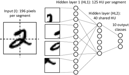
Figure 7: “Multi-modal” setting for the MNIST dataset.

Training mode			Errors	# of parameters
Dropout, 784-1200-1200-10 [53]			107	2395210	N
Dropout, 784-500-40-10 (ours)			119	412950	0.17N
${a^{2}}^{2}$(a) Fully connected setting
Pretraining (HL1)	Dropout (I)	ModDrop (I)	Errors	# of parameters
no	no	no	142	118950	$0.05N$
no	yes	no	123
yes	no	no	118
yes	yes	no	102
yes	yes	yes	102
${a^{2}}^{2}$(b) “Multi-modal” setting, $196{\times}4$-$125{\times}4$-40-10

TABLE VII: Experiments on the MNIST dataset.

Training mode	Dropout	Dropout + ModDrop
Missing segments, test error, %
All segments visible	1.02	1.02
1 segment covered	10.74	2.30
2 segments covered	35.91	7.19
3 segments covered	68.03	24.88
Pepper noise 50% on segments, test error, %
All clean	1.02	1.02
1 corrupted segment	1.74	1.56
2 corrupted segments	2.93	2.43
3 corrupted segments	4.37	3.56
All segments corrupted	7.27	6.42

TABLE VIII: Effect of ModDrop training under occlusion and noise.

Currently, the state-of-the-art for a fully-connected 782-1200-1200-10 network with dropout regularization (50% for hidden units and 20% for the input) and tanh activations [53] is 107 errors on the MNIST test set (see Table VII). In this case, the number of units in the hidden layer is unnecessarily large, which is exploited by dropout-like strategies. When real-time performance is a constraint, this redundancy in the number of operations becomes a serious limitation. Instead, switching to our tree-structured network (i.e. a network with separated modality-specific input layers connected to a set of shared layers) is helpful for independent modality-wise tuning of model capacity, which in this case does not have to be uniformly distributed over the input units. For this multi-modal setting we optimized the number of units (125) for each channel and do not apply dropout to the hidden units (which in this case turns out to be harmful due to the compactness of the model), limiting ourselves to dropping out the inputs at a rate of 20%. In addition, we apply ModDrop on the input, where the probability of each segment to be dropped is 10%.

The results in Table VII show that separate pretraining of modality-specific paths generally yields better performance and leads to a significant decrease in the number of parameters due to the capacity restriction placed on each channel. This is apparent in the 4^th row of Table VIIb: with pretraining, better performance (102 errors) is obtained with 20 times less parameters.

MNIST results under occlusion and noise are presented in Table VIII. We see that ModDrop, while not affecting the overall performance on MNIST, makes the model significantly less sensitive to occlusion and noise.

7.5.2 Experiments on ChaLearn 2014 LAP with audio

mPretrainingm	mDropoutm	mInitial.m	mModDropm	mAccuracy, %m
no	no	no	no	$91.94$
no	yes	no	no	$93.33$
yes	no	no	no	$94.96$
yes	yes	no	no	$96.31$
yes	yes	yes	no	$96.77$
yes	yes	yes	yes	$\mathbf{96.81}$

TABLE IX: Comparison of different training strategies on the ChaLearn 2014 LAP dataset augmented with audio.

In a real multi-modal setting, optimizing and balancing a tree-structured architecture is an extremely difficult task as its separated parallel paths vary in complexity and operate on different feature spaces. The problem becomes even harder under the constraint of real-time performance and, consequently, the limited capacity of the network.

Our experiments have shown that insufficient modelling capacity of one of the modality-specific subnetworks leads to a drastic degradation in performance of the whole system due to the multiplicative nature of the fusion process. Those bottlenecks are typically difficult to find without thorough per-channel testing.

We propose to start by optimizing the architecture and hyper-parameters for each modality separately through discriminative pretraining. During fusion, input paths are initialized with pretrained values and fine-tuned while training the output shared layers.

Furthermore, the shared layers can also be initialized with pretrained diagonal blocks as described in Section 4, which results in a significant speed up in the training process. We have observed that in this case, setting the biases of the shared hidden layer is critical in converging to a better solution.

As in the case of the MNIST experiments, we apply 20% dropout on the input signal and ModDrop with probability of 10% (optimized on the validation set). As before, dropping hidden units during training led to degradation in performance of our architecture due to its compactness.

A comparative analysis of the efficiency of various training strategies is reported in Table IX. Here, we provide validation error of per dynamic pose classification as a direct indicator of convergence of training. The “Pretraining” column corresponds to modality-specific paths while “Initial.” indicates whether or not the shared layers have also been pre-initialized with pretrained diagonal blocks. In all cases, dropout (20%) and ModDrop (10%) are applied to the input signal. Accuracy corresponds to per-block classification on the validation set.

Differences in effectiveness of different strategies agree well with what we have observed previously on MNIST. Modality-wise pretraining and regularization of the input have a strong positive effect on performance. Interestingly, in this case ModDrop resulted in further improvement in scores even for the complete set of modalities (while increasing the dropout rate did not have the same effect).

Analysis of the network behaviour in conditions of noisy or missing signals in one or several channels is provided in Table X. Once again, ModDrop regularization resulted in much better network stability with respect to signal corruption and loss.

Modality	Dropout		Dropout + ModDrop
	Accuracy, %	Jaccard index	Accuracy, %	Jaccard index
All present	96.77	0.876	96.81	0.880
Missing signals in separate channels
Left hand	89.09	0.826	91.87	0.832
Right hand	81.25	0.740	85.36	0.796
Both hands	53.13	0.466	73.28	0.680
Mocap	38.41	0.306	92.82	0.859
Audio	84.10	0.789	92.59	0.854
Pepper noise 50% in channels
Left hand	95.36	0.874	95.75	0.874
Right hand	95.48	0.873	95.92	0.874
Both hands	94.55	0.872	95.06	0.875
Mocap	93.31	0.867	94.28	0.878
Audio	94.76	0.867	94.96	0.872

TABLE X: Effect of ModDrop on ChaLearn 2014+audio.

8 Conclusion

We have described a generalized method for gesture and near-range action recognition from a combination of range video data and articulated pose. Each of the visual modalities captures spatial information at a particular spatial scale (such as motion of the upper body or a hand), and the whole system operates at two temporal scales.

The model can be further extended and augmented with arbitrary channels (depending on available sensors) by introducing additional parallel pathways without significant changes in the general structure. We illustrate this concept by augmenting video with speech. Multiple spatial and temporal scales per channel can easily be integrated.

Finally, we have explored various aspects of multi-modal fusion in terms of joint performance on a complete set of modalities as well as robustness of the classifier with respect to noise and dropping of one or several data channels. As a result, we have proposed a modality-wise regularisation strategy (ModDrop) allowing our model to obtain stable predictions even when inputs are corrupted.

Acknowledgement

This work has been partly financed through the French grant Interabot, a project of type “Investissement’s d’Avenir / Briques Génériques du Logiciel Embarqué”.

Natalia Neverova is a PhD student at INSA de Lyon and LIRIS (CNRS, France) working in the area of gesture and action recognition with emphasis on multi-modal aspects and deep learning methods. She is advised by Christian Wolf and Graham Taylor, and her research is a part of Interabot project in partnership with Awabot SAS. She was a visiting researcher at University of Guelph in 2014 and at Google in 2015.

Christian Wolf is assistant professor at INSA de Lyon and LIRIS, CNRS, since 2005. He is interested in computer vision and machine learning, especially the visual analysis of complex scenes in motion, structured models, graphical models and deep learning. He received his MSc in computer science from Vienna University of Technology in 2000, and a PhD from the National Institute of Applied Science (INSA de Lyon), in 2003. In 2012 he obtained the habilitation diploma.

Graham Taylor is an assistant professor at University of Guelph. He is interested in statistical machine learning and biologically-inspired computer vision, with an emphasis on unsupervised learning and time series analysis. He completed his PhD at the University of Toronto in 2009, where his thesis co-advisors were Geoffrey Hinton and Sam Roweis. He did a postdoc at NYU with Chris Bregler, Rob Fergus, and Yann LeCun.

Florian Nebout is a project manager at Awabot, leading different robotics projects, which are mostly dedicated to remote presence applications. He is especially interested in human robot interaction and how robotics can change our daily life. He graduated from INSA de Lyon, France and worked at CSIRO Human Computer Interaction team and ANU Information and Human Centred Computing Research Group in Canberra, Australia.

References

- [1] R. Girshick, J. Donahue, T. Darrell, and J. Malik, “Rich feature hierarchies for accurate object detection and semantic segmentation,” in CVPR, 2014.
- [2] P. Sermanet, D. Eigen, X. Zhang, M. Mathieu, R. Fergus, and Y. LeCun, “OverFeat: Integrated Recognition, Localization and Detection using Convolutional Networks,” in ICLR, 2014.
- [3] A. Krizhevsky, I. Sutskever, and G. Hinton, “ImageNet Classification with Deep Convolutional Neural Networks,” in NIPS, 2012.
- [4] C. Farabet, C. Couprie, L. Najman, and Y. LeCun, “Learning Hierarchical Features for Scene Labeling,” in PAMI, 2013.
- [5] C. Couprie, F. Clément, L. Najman, and Y. LeCun, “Indoor Semantic Segmentation using depth information,” in ICLR, 2014.
- [6] Y. LeCun, L. Bottou, Y. Bengio, and P. Haffner, “Gradient-based learning applied to document recognition,” Proceedings of the IEEE, vol. 86, no. 11, pp. 2278–2324, 1998.
- [7] S. E. Kahou et al., “Combining modality specific deep neural networks for emotion recognition in video,” in ICMI, 2013.
- [8] Y. Taigman, M. Yang, M. A. Ranzato, and L. Wolf, “DeepFace: Closing the Gap to Human-Level Performance in Face Verification,” in CVPR, 2014.
- [9] M. Baccouche, F. Mamalet, C. Wolf, C. Garcia, and A. Baskurt, “Spatio-Temporal Convolutional Sparse Auto-Encoder for Sequence Classification,” in BMVC, 2012.
- [10] A. Karpathy, G. Toderici, S. Shetty, T. Leung, R. Sukthankar, and F.-F. Li, “Large-scale Video Classification with Convolutional Neural Networks,” in CVPR, 2014.
- [11] K. Simonyan and A. Zisserman, “Two-Stream Convolutional Networks for Action Recognition in Videos,” in arXiv:1406.2199v1, 2014.
- [12] A. Jain, J. Tompson, Y. LeCun, and C. Bregler, “MoDeep: A Deep Learning Framework Using Motion Features for Human Pose Estimation,” in ACCV, 2014.
- [13] F. Zhou, F. De la Torre, and J.-K. Hodgins, “Hierarchical Aligned Cluster Analysis for Temporal Clustering of Human Motion,” in PAMI, 2013.
- [14] S. Escalera, X. Baró, J. Gonzàlez, M. Bautista, M. Madadi, M. Reyes, V. Ponce, H. Escalante, J. Shotton, and I. Guyon, “ChaLearn Looking at People Challenge 2014: Dataset and Results,” in ECCVW, 2014.
- [15] H. Wang, A. Kläser, C. Schmid, and C.-L. Liu, “Dense trajectories and motion boundary descriptors for action recognition,” IJCV, 2013.
- [16] J. Shotton, A. Fitzgibbon, M. Cook, T. Sharp, M. Finocchio, R. Moore, A. Kipman, and A. Blake, “Real-time human pose recognition in parts from single depth images,” in CVPR, 2011.
- [17] C. Keskin, F. Kiraç, Y. Kara, and L. Akarun, “Real time hand pose estimation using depth sensors,” in ICCV Workshop, 2011.
- [18] D. Tang, T.-H. Yu, and T.-K. Kim, “Real-time Articulated Hand Pose Estimation using Semi-supervised Transductive Regression Forests,” in ICCV, 2013.
- [19] D. Tang, H. J. Chang, A. Tejani, and T.-K. Kim, “Latent Regression Forest: Structured Estimation of 3D Articulated Hand Posture,” in CVPR, 2014.
- [20] J. Tompson, M. Stein, Y. LeCun, and K. Perlin, “Real-Time Continuous Pose Recovery of Human Hands Using Convolutional Networks,” in ACM Transaction on Graphics, 2014.
- [21] N. Neverova, C. Wolf, G. Taylor, and F. Nebout, “Hand segmentation with structured convolutional learning,” in ACCV, 2014.
- [22] I. Oikonomidis, N. Kyriazis, and A. Argyros, “Efficient model-based 3D tracking of hand articulations using Kinect,” in BMVC, 2011.
- [23] C. Qian, X. Sun, Y. Wei, X. Tang, and J. Sun, “Realtime and Robust Hand Tracking from Depth,” in CVPR, 2014.
- [24] F. Wang and Y. Li, “Beyond Physical Connections: Tree Models in Human Pose Estimation,” in CVPR, 2013.
- [25] X. Chen, R. Mottaghi, X. Liu, S. Fidler, R. Urtasun, and A. Yuille, “Detect What You Can: Detecting and Representing Objects using Holistic Models and Body Parts,” in CVPR, 2014.
- [26] J. Wang, Z. Liu, Y. Wu, and J. Yuan, “Mining actionlet ensemble for action recognition with depth cameras,” in CVPR, 2012.
- [27] J. Sung, C. Ponce, B. Selman, and A. Saxena, “Unstructured Human Activity Detection from RGBD Images,” in ICRA, 2012.
- [28] X. Chen and M. Koskela, “Online RGB-D gesture recognition with extreme learning machines,” in ICMI, 2013.
- [29] C. Monnier, S. German, and A. Ost, “A Multi-scale Boosted Detector for Efficient and Robust Gesture Recognition,” in ECCVW, 2014.
- [30] J. Y. Chang, “Nonparametric Gesture Labeling from Multi-modal Data,” in ECCV Workshop, 2014.
- [31] K. Nandakumar et al., “A Multi-modal Gesture Recognition System Using Audio, Video, and Skeletal Joint Data Categories and Subject Descriptors,” in ICMI Workshop, 2013.
- [32] Q. V. Le, W. Y. Zou, S. Y. Yeung, and A. Y. Ng, “Learning hierarchical invariant spatio-temporal features for action recognition with independent subspace analysis,” in CVPR, 2011.
- [33] M. Ranzato, F. J. Huang, Y.-L. Boureau, and Y. LeCun, “Unsupervised Learning of Invariant Feature Hierarchies with Applications to Object Recognition,” in CVPR, 2007.
- [34] B. Chen, J.-A. Ting, B. Marlin, and N. de Freitas, “Deep learning of invariant Spatio-Temporal Features from Video,” in NIPSW, 2010.
- [35] S. Ji, W. Xu, M. Yang, and K. Yu, “3D Convolutional Neural Networks for Human Action Recognition,” PAMI, 2013.
- [36] L. Pigou, S. Dieleman, and P.-J. Kindermans, “Sign Language Recognition Using Convolutional Neural Networks,” in ECCVW, 2014.
- [37] D. Wu, “Deep Dynamic Neural Networks for Gesture Segmentation and Recognition,” in ECCV Workshop, 2014.
- [38] F. Bach, G. Lanckriet, and M. Jordan, “Multiple Kernel Learning, Conic Duality, and the SMO Algorithm,” in ICML, 2004.
- [39] P. Gehler and S. Nowozin, “On Feature Combination for Multiclass Object Classification,” in ICCV, 2009.
- [40] G. Ye, D. Liu, I.-H. Jhuo, and S.-F. Chang, “Robust Late Fusion With Rank Minimization,” in CVPR, 2012.
- [41] P. Natarajan, S. Wu, S. Vitaladevuni, X. Zhuang, S. Tsakalidis, U. Park, R. Prasad, and P. Natarajan, “Multimodal Feature Fusion for Robust Event Detection in Web Videos,” in CVPR, 2012.
- [42] J. Ngiam, A. Khosla, M. Kin, J. Nam, H. Lee, and A. Y. Ng, “Multimodal deep learning,” in ICML, 2011.
- [43] N. Srivastava and R. Salakhutdinov, “Multimodal learning with Deep Boltzmann Machines,” in NIPS, 2013.
- [44] Z. Wu, Y.-G. Jiang, J. Wang, J. Pu, and X. Xue, “Exploring Inter-feature and Inter-class Relationships with Deep Neural Networks for Video Classification,” in ACM Multimedia, 2014.
- [45] N. Neverova, C. Wolf, G. Paci, G. Sommavilla, G. W. Taylor, and F. Nebout, “A multi-scale approach to gesture detection and recognition,” in ICCV Workshop, 2013.
- [46] A. Hernandez-Vela et al., “Probability-based Dynamic Time Warping and Bag-of-Visual-and-Depth-Words for Human Gesture Recognition in RGB-D,” in Pattern Recognition Letters, 2014.
- [47] N. Neverova, C. Wolf, G. Taylor, and F. Nebout, “Multi-scale deep learning for gesture detection and localization,” in ECCVW, 2014.
- [48] M. Zanfir, M. Leordeanu, and C. Sminchisescu, “The Moving Pose: An Efficient 3D Kinematics Descriptor for Low-Latency Action Recognition and Detection,” in ICCV, 2013.
- [49] L. Deng, J. Li, J. Huang, K. Yao, D. Yu, F. Seide, M. Seltzer, G. Zweig, X. He, J. Williams, Y. Gong, and A. Acero, “Recent advances in deep learning for speech recognition at Microsoft,” in ICASSP, 2013.
- [50] L. A. Alexandre, A. C. Campilho, and M. Kamel, “On combining classifiers using sum and product rules,” in Pattern Recognition Letters, no. 22, 2001, pp. 1283–1289.
- [51] I. J. Goodfellow, D. Warde-Farley, M. Mirza, A. Courville, and Y. Bengio, “Maxout Networks,” in arXiv:1302.4389v4, 2013.
- [52] P. Baldi and P. Sadowski, “The dropout learning algorithm,” Journal of Artificial Intelligence, vol. 210, pp. 78–122, 2014.
- [53] G. E. Hinton, N. Srivastava, A. Krizhevsky, I. Sutskever, and R. R. Salakhutdinov, “Improving neural networks by preventing co-adaptation of feature detectors,” in arXiv:1207.0580, 2012.
- [54] S. Wang and C. Manning, “Fast dropout training,” in ICML, 2013.
- [55] E. L. Lehmann, “Elements of Large-Sample Theory,” in ICML, 1998.
- [56] K. Fang, W. Gao, and D. Zhao, “Large-Vocabulary Continuous Sign Language Recognition Based on Transition-Movement Models,” in IEEE Transactions on Systems, Man, and Cybernetics, 2007.
- [57] S. Escalera et al., “Multi-modal Gesture Recognition Challenge 2013: Dataset and Results,” in ICMI workshop, 2013.
- [58] J. Bergstra et al., “Theano: A CPU and GPU Math Expression Compiler,” in Proceedings of the Scipy Conference, 2010.
- [59] P. Geurts, D. Ernst, and L. Wehenkel, “Extremely randomized trees,” in Machine learning, 63(1), 3-42, 2006.
- [60] A. Lee, T. Kawahara, and K. Shikano, “Julius - an open source real-time large vocabulary recognition engine,” in Interspeech, 2001.
- [61] N. Camgoz, A. Kindiroglu, and L. Akarun, “Gesture Recognition using Template Based Random Forest Classifiers,” in ECCVW, 2014.
- [62] G. Evangelidis, G. Singh, and R. Horaud, “Continuous gesture recognition from articulated poses,” in ECCV Workshop, 2014.
- [63] X. Peng, L. Wang, and Z. Cai, “Action and Gesture Temporal Spotting with Super Vector Representation,” in ECCVW, 2014.
- [64] G. Chen, D. Clarke, M. Giuliani, D. Weikersdorfer, and A. Knoll, “Multi-modality Gesture Detection and Recognition With Un-supervision, Randomization and Discrimination,” in ECCVW, 2014.
- [65] Y. LeCun, L. Bottou, Y. Bengio, and P. Haffner, “Gradient-based learning applied to document recognition,” in Proceedings of the IEEE, vol. 86(11), 1998, pp. 2278–2324.