Methods and Metrics for Fair Server Assessment
under Real-Time Financial Workloads

Abstract

Energy efficiency has been a daunting challenge for datacenters. The financial industry operates some of the largest datacenters in the world. With increasing energy costs and the financial services sector growth, emerging financial analytics workloads may incur extremely high operational costs, to meet their latency targets. Microservers have recently emerged as an alternative to high-end servers, promising scalable performance and low energy consumption in datacenters via scale-out. Unfortunately, stark differences in architectural features, form factor and design considerations make a fair comparison between servers and microservers exceptionally challenging.

In this paper we present a rigorous methodology and new metrics for fair comparison of server and microserver platforms. We deploy our methodology and metrics to compare a microserver with ARM cores against two servers with x86 cores, running the same real-time financial analytics workload. We define workload-specific but platform-independent performance metrics for platform comparison, targeting both datacenter operators and end users.

Our methodology establishes that a server based the Xeon Phi processor delivers the highest performance and energy-efficiency. However, by scaling out energy-efficient microservers, we achieve competitive or better energy-efficiency than a power-equivalent server with two Sandy Bridge sockets, despite the microserver’s slower cores. Using a new iso-QoS (iso-Quality of Service) metric, we find that the ARM microserver scales enough to meet market throughput demand, i.e. a 100% QoS in terms of timely option pricing, with as little as 55% of the energy consumed by the Sandy Bridge server.

¹The School of Electronics, Electrical Engineering and Computer Science, Queen’s University Belfast, Northern Ireland BT7 1NN, United Kingdom ²The Institute for Electronics Communications and Information Technology, Queen’s University Belfast, The Northern Ireland Science Park Queen’s Road, Belfast, Northern Ireland BT3 9DT, United Kingdom ³Neueda Consulting Limited, Glenwood Business Centre, Springbank Industrial Estate Belfast, Northern Ireland BT17 0QL, United Kingdom

KEY WORDS:Event processing, numerical simulation, energy efficiency, financial analytics, datacenters, kernels

1 Introduction

Financial analytics are one of the most important services in modern capital markets. Real-time financial analytics, such as option pricing and trading risk assessment incur a high premium on top of basic service costs, due to their latency criticality.

Financial service providers operate datacenters which are co-located with market data feeds, to meet the low latency requirements of real-time analytics. These datacenters incur extraordinarily high cost of ownership due to hardware overprovisioning, their scale, and their carbon footprint. The choice of compute server architecture for these datacenters fundamentally dictates their cost of ownership and sustainability. Unfortunately, the financial industry lacks concrete methodologies and metrics for fair assessment of server architectures as computational workhorses for emerging analytics workloads.

In this paper we present a rigorous methodology and a set of metrics for evaluation of server performance and energy efficiency under real-time financial analytics workloads. We base our work on an earlier contribution which explored the viability of an ARM microserver in comparison to Intel Sandy Bridge servers for real-time option pricing workloads [1]. We introduce a platform-independent workload setup and optimization methodology, in conjunction with platform-independent metrics of performance, energy-efficiency and quality of service. We leverage these tools to fairly and thoroughly compare three server architectures that represent vastly different price, cost, performance and power trade-offs: a Calxeda ECX-1000 microserver [2] based on ARM Cortex A9 cores; a Dell server based on Intel Sandy Bridge cores; and a Dell server based on an Intel Xeon Phi co-processor.

Our methodology yields important and often counter-intuitive findings. We establish that a server based the Xeon Phi processor delivers the highest performance and energy-efficiency. However, by scaling out energy-efficient ARM microservers within a 2U rack-mounted unit, we achieve competitive or better energy-efficiency than a power-equivalent server with two Intel Sandy Bridge sockets, despite the microserver’s slower cores. Using a new iso-QoS (iso-Quality of Service) metric, we find that the ARM microserver scales enough to meet market throughput demand, i.e. a 100% QoS in terms of timely option pricing, with as little as 55% of the energy consumed by the Sandy Bridge server.

Using the same C and SIMD code basis, we uncover several more findings of interest. The servers exhibit vast differences in energy-efficiency due to differences in the implementation of transcendental functions in hardware, as well as the implementation of vector units and ISAs. We find that power saving modes employing DVFS are invariably less energy-efficient than performance boosting modes for financial analytics workloads. We also find that while servers exhibit good performance scaling with more cores, they also exhibit non-ideal energy scaling, thus providing an opportunity for energy conservation via throttling concurrency.

The paper begins by providing background on microservers and server comparison methodologies (Section 2). We proceed by briefly defining financial option contracts and explaining the computational methods that we have used to obtain contract prices from spot prices in our real-time workloads (Section 3). We discuss common code optimization and vectorization methodology (Section 4). We move on to details of the platforms which we used for our study and present our experimental and measurement methodology and metrics (Section 5). We proceed by presenting results from standalone kernel experiments using an actual stock market feed (Section 6). We delve into a discussion of our study findings. We then present and analyze results from production-strength experiments (Section 7). We discuss related work (Section 8) and finish the paper with summarizing our conclusions (Section 9).

2 Background

Microservers have the potential to reduce the energy consumption of datacenters by using low-power processors designed for the embedded systems market [3]. Back-of-the-envelope estimates suggest that microserver processors such as the Samsung Exynos and Calxeda Highbank ECX-1000 [2] consume 5 to 30 times less power than high-end server-class counterparts, such as Intel’s Sandy Bridge and are 5 to 15 times more energy-efficient in integer performance per Watt [4, 5]. However, microserver processors are limited in floating point performance and SIMD/SIMT acceleration capabilities [3].

In comparing servers to microservers, one must find a fair and unbiased methodology. A challenge lies in that a standalone microserver represents a vastly different price, performance and operating power point than a standalone server.

2.1 Metric considerations

We stipulate that a comparison methodology should be platform neutral and ascertain that the server architectures under consideration meet the same, tangible target, be it performance, Quality of Service (QoS), power consumption, or energy consumption. We thus allow scale-out or scale-up of each server to meet the set target, while comparing other metrics of interest to rank the servers. Furthermore, the metrics used should reflect workload fluctuation, but not be unduly influenced by non-deterministic environmental, hardware or system artifacts. Finally, we stipulate that any comparison should be based on the same code base, developed with similar coding effort on each server. We elaborate on this issue in the following section.

2.2 Workload coding considerations

We use real-time option pricing workloads, which represent one of the most important and performance-critical domains of financial analytics. Option pricing is an inherently parallel problem, as each option contract is defined over a single stock, independently. A portable implementation with similar effort across servers described in our earlier work [1], exploits parallelism in the workload by using UDP multicast channels to distribute prices and POSIX threads to distribute option pricing instances between cores and their hardware contexts, if present.

In addition we use the same code base to exploit the vector processing units available on each server and further accelerate the numerical calculations in our workloads. Our code base uses manual loop unrolling and vectorization using pragmas. Our implementation is expressed in the C language, which is the norm in computational finance. The C language standard presents a number of challenges for implicit vectorization by a compiler [6]. Principal among these challenges are the facts that C imposes no constraints on subroutine argument aliasing, the “for” statement permits loop bounds and increment to change within the loop and loop operations are often implemented with pointers, which could be aliased or point to overlapping areas of memory. We demonstrate significant differences in auto-vectorization capabilities between compilers. These differences render autovectorization inappropriate for fair server comparison, even though on occasion (e.g. ICC on the Xeon Phi), autovectorization produces excellent results.

On the other hand, C compilers provide implicit vectorization with associated pragmas and command line options to control the vectorization process. These features help the authoring of portable SIMD code and we leverage them in this work. Still, there is no common standard for compilers to abide by to provide the same quality of vectorization nor is there a method to enforce different compilers to produce comparable vectorization output. We offer insights on how to address this problem in our methodology. Manual vectorization has been extensively used in production environments [7, 8, 9, 10, 11] but remains heavily dependent on programmer skill.

3 Computing Option Prices

In finance, the term Option means a derivative product which is a contract giving the holder the right to either buy (Call option) or to sell (Put option) one or more underlying assets, such as a fixed number of shares in a company, for a defined price and either on or before a contract end date. An Options contract, unlike a Futures contract, does not impose an obligation on the holder to exercise their right. There are several types of Options distinguished by the terms in their contract. We construct real-time analytics workloads that continuously execute Monte Carlo or Binomial Tree option pricing models. These can price both the so-called exotic American or Bermudan options as well as European options. We focus on European options for which the Black-Scholes equation provides a closed form solution, against which our results can be compared for accuracy.

Black and Scholes [12, 13] proposed a second-order partial differential equation which models the variation of the price of a European vanilla option, contractual strike price $P$, over time in years $T$, assuming that:

• the underlying asset price (spot price), $S$ follows a log normal distribution,

• the volatility $\sigma$ of $S$ is constant and

• the risk free interest rate, or rate of return, $r$, expressed with continuous compounding is constant.

Under these conditions an analytic solution is:

$${\rm Price}=(-1)^{p}\left(SN((-1)^{p}d_{1})-P{\rm e}^{-rT}N((-1)^{p}d_{2})\right)$$ (1)

In this equation $p=1$ for a Call option and $p=0$ for a Put option and $d_{1}$ and $d_{2}$ are defined by:

$$d_{1}=\frac{1}{\sigma\sqrt{T}}\left(\log\left(\frac{S}{N}\right)+\frac{r+\sigma^{2}}{2}\;T\right)\;\;\;\;{\rm and}\;\;\;\;d_{2}=d_{1}-\sigma\sqrt{T}$$ (2)

where $N(x)$ is the cumulative normal distribution function (CDF).

Moving beyond the limitations of the Black-Scholes model, the price of an option on any given date can be modeled using stochastic calculus, essentially simulating the path of the underlying variables over a set of paths within a time window. Analytical solutions for the stochastic equations are not generally possible so that a variety of computational numerical solution methods have been developed. European vanilla options can also be priced using these numerical methods. We apply two models, with distinct computational characteristics, as described next.

3.1 Monte Carlo (MC)

At the center of a Monte Carlo simulation of option pricing is a rate-limiting for-loop, an aspect that it shares in common with HPC applications in many fields. For a Put option the formula is [14]:

$${\rm Price}=\frac{{\rm e}^{-rT}}{N}\sum_{i=1}^{N}\max\left(0,S-P{\rm e}^{(r-\frac{\sigma^{2}}{2})T+\sigma\sqrt{T}x_{i}}\right)$$ (3)

In equation 3, ${x_{i}\ (i=1\ldots N)}$ are a set of random numbers drawn from the standard normal distribution. The formula for a Call option is similar to the Put option.

Given that $\sigma,r$ and $T$ are constant within the context of the loop, the implementation of equation 3 creates a compute bound process dominated by the exponential function, with relatively few loads and stores to memory. One bottleneck is the control of numerical round-off error associated with a floating point summation process over a large number of terms [15, 16]. Another is the generation of sets of good quality pseudo-random numbers (PRN) because the computed price converges only slowly as $O\left(\frac{1}{\sqrt{N}}\right)$. This is significant because the operation count during execution of the for-loop code scales as $O(N)$. In our work, uniform random numbers are generated using the 32-bit version of the Mersenne Twister algorithm [17], then transformed to a standard normal distribution using the Box-Muller formula.

3.2 Binomial Tree (BT)

The binomial tree option pricing model [18] builds a lattice of options prices with a root node at the starting date and multiple nodes at the end date. The model decomposes the time variable into discrete steps, each corresponding to a level in the lattice. The price can be computed at any level in the tree, which corresponds to an intermediate date within the contract, thereby making the binomial model suitable for pricing American and Bermudan options. In general at each time point $i$, there is a vector of option prices computed, $S_{ij}$. Given price $S_{ij}$ and a pair of factors $u$ and $d$ representing the up and down movements, the two possible prices at the next level are $S_{(i+1)j}=uS_{ij}$ and $S_{(i+1)(j+1)}=dS_{ij}$ where the factors $u,d$ are constant across the tree and are formally defined as:

$$u={\rm e}^{\sigma\sqrt{T}}\;\;\;\ {\rm and}\;\;\;\;d=\frac{1}{u}$$ (4)

The complete algorithm therefore has three steps:

• Given $S_{0}$, the current spot price, work forward from today, the date of computation, to the expiration date (timepoint N), applying the up and down factors at each step and thereby computing all final node prices $S_{Nj}$.

• At each final node of the tree (level $n$) compute the exercise value.

• Iterate backwards from the final nodes in the tree and for every intermediate node compute the option price assuming risk neutrality, which means that the price is computed as the discounted value of the future payoff.

The final step; a nested for-loop, dominates the time taken by the computation. The number of updates performed scales as $O(\frac{N^{2}}{2})$ with each update consisting of two floating point multiplications and one floating point addition. This contrasts with the MC algorithm, where there is a need to repeatedly compute transcendental mathematical functions. The convergence of the method is a function of the number of timesteps chosen for the computations.

It is not necessary to hold all of the prices $S_{ij}$ in memory at the same time. Only the prices at timepoint $i$ are needed. A vector with the elements being overwritten as the values are processed during the backwards iteration process suffices for this purpose. The BT implementation is thus dominated by pointer dereferencing to generate array indices and by data move activity, in contrast to the random number selection and sum reduction characteristics of the MC algorithm.

4 Optimization Methodology

In this section we discuss a common set of optimizations applied to our workload to tune performance. These include algorithmic optimizations and platform-dependent optimizations through unrolling and vectorization, either by the compiler or via explicit use of vector instructions. We develop a common, platform-independent methodology for these optimizations and discuss any platform-dependent implementation needs, where necessary.

We developed the initial code base in the C language to be used on all servers for the experiments. The heart of our system is an OptionPricer implementing the algorithms described in Section 3. We manually unrolled the loops and used the same vectorized algorithm on each server, albeit with modifications to accommodate different widths of the vector ISA supported on each server. The common approach to vectorization on all platforms, using either the compiler or a direct algorithmic translation to vector code, reflects similar optimization effort on each server and is the fairest way to perform a comparison among servers.

4.1 Algorithmic optimization for Monte Carlo

In its usual form, the Monte Carlo kernel is a for-loop over a set of normally distributed random numbers, $x_{i}$. The loop applies a formula to each number, followed by a summation. Within the loop, each random number is used to compute a payoff value, a process which involves the relatively expensive evaluation of an exponential function. If this value is positive then it contributes to the sum otherwise it is discarded. This means that an if-statement dominates the loop. This algorithmic feature hampers further performance and power efficiency optimizations, as will be amply clear in the results section. Given that all variables in the payoff expression, except the random number, are loop-invariant, a threshold, ${\rm Thres}$ for pre-screening the random numbers can be applied. For Call options this is defined as:

$${\rm Thres}=\frac{1}{\sigma\;\sqrt{(}T)}\;{\rm\log}_{\rm e}\frac{\rm strike\;price}{{\rm stockPx}{\rm e}^{(r-\frac{\sigma^{2}T}{2})}}$$ (5)

such that the payoff value is computed using only values $x_{i}$ where:

$$x_{i}>{\rm Thres}$$ (6)

The impact of this screening on any given option contract evaluation depends on the specific values of stock and strike prices, interest rate, volatility and time to expiry.

On one hand, screening random numbers as above leads to a further algebraic simplification allowing several multiply operations to be factored outside the sum loop, which now becomes:

$$\sum_{j=1}^{M}{\rm e}^{\sigma\sqrt{(}T)\;x_{j}}$$ (7)

where $M$ is the number of random numbers passing the threshold test defined in Equation 5. On the other hand, this prevents complete vectorization of random number generation within the compute intensive part, which is also dependent on the input data.

4.2 Vectorization

Server processors have diverse vector ISAs and vector unit implementations. In this section we discuss whether and how this diversity can be overcome with a common approach for each of our two financial analytics kernels.

4.2.1 Monte Carlo

We leverage the Cephes software library [19] in our vectorization exercise. The library is an open source collection of high quality mathematical routines written in C. These routines have been tested for over thirty years in scientific and engineering applications. The library presents a common reference, open source alternative to vendor specific libraries and to the math library supplied by each C compiler. It implements versions of the $sin$, $cos$, $exp$ and $log$ functions tailored for different vector units including Intel’s SSE and AVX as well as ARM’s NEON.

We outline the Monte Carlo kernel vectorization using the Intel SSE instruction set as an example. The SSE instructions operate on 128-bit wide registers, named XMM registers, while the exponential function uses single-precision floating point variables, each 32-bits wide. This means that four separate values are computed in parallel in a single SSE $exp$ instruction using one XMM register. The sum loop, shown in Equation 7, is transformed to perform one fourth of the iterations due to the vectorized exponential calculation. Note the ARM NEON registers are 128-bit wide too and apart from calling the NEON-specialized exponential function, code changes are identical to Intel’s SSE. For the AVX implementation, YMM registers extend XMM registers to be 256 bits wide, thus it is possible to compute eight values in parallel. The loop is further transformed to accommodate this extra opportunity. A further optimization that we have not implemented here, would be to extend the vectorized exponential routine to use several more vector registers in a single invocation. This could further improve performance by reducing the number of iterations in the sum loop and the associated overhead. It could also provide additional gains by leveraging better locality on cached data.

4.2.2 Binomial Tree

The binomial tree computation is dominated by an innermost loop which processes the set of all values at each timestep to generate values for a previous timestep. A loop step can be expressed simply as

$$x_{i}=ax_{i}+bx_{i+1}$$ (8)

This loop step relation shows that there is an anti-dependency between iterations. This dependency needs to be removed in order to enable vectorization. Notably, the GCC compiler failed to recognize this vectorizing opportunity on all our platforms, because of this dependency. The Intel compiler (ICC) was able to overcome this barrier and produce vectorized code on the Phi and Sandy Bridge servers.

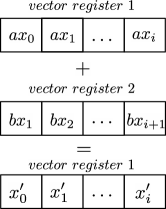
Figure 1: Vectorization of Binomial Tree kernel

We have constructed two handcrafted vectorized solutions for the kernel: one which replaces the inner loop entirely by invoking a routine written in vectorized assembly, and another using compiler vector intrinsics placed inline with the C source code. The latter are referred to as INTRINSICS_xxx build and runs, where xxx depends on the platform. These two handcrafted vectorization solutions overcome the apparent anti-dependency and enable us to compare the low-level manual assembly solution versus a more abstract, intrinsic-based vectorization method. Both versions employ loop unrolling in conjunction with vectorization to calculate more values in a single iteration. Figure 1 shows schematically the vectorized BT calculation. The unroll factor is equal to the vector register width measured in double-precision floating point numbers (single-precision in the case of the ARM Cortex A9 NEON unit). Similarly to the Monte Carlo algorithm, we present a detailed example of vectorizing the BT calculation, using the the SSE 128-bit instruction set as an example. The sequence of vectorization steps is as follows:

• Preload high and low double words of xmm10 with value $a$, and xmm11 with $b$.

• Populate vector registers xmm0,1,2,3 with eight double precision (64-bit) contiguous values, two per register.

• Copy xmm0,1,2,3 to xmm5,6,7,8 and downshift the eight values, using register shift and OR operations.

• Load one value to fill the gap at xmm8 caused by the downshift.

• Execute the four products and summations given symbolically by

  $$xmm0=xmm0\cdot xmm10+xmm5\cdot xmm11$$

  $$xmm1=xmm1\cdot xmm10+xmm6\cdot xmm11$$

  $$xmm2=xmm2\cdot xmm10+xmm7\cdot xmm11$$

  $$xmm3=xmm3\cdot xmm10+xmm8\cdot xmm11$$

• Write the registers xmm0,1,2,3 to RAM

• Repeat the steps above for as many sets of eight values as exist in the loop.

We follow a similar vectorization approach for the ARM NEON 128-bit vector ISA, the Intel AVX 256-bit vector ISA and the Intel Xeon Phi Knight’s Corner (KNC) 512-bit vector ISA. A difference between the Intel family and ARM NEON vector units is that NEON supports only single-precision floating point vector operations. Therefore, the vectorized calculation of Binomial Tree on ARM has double the throughput of SSE and effectively the same throughput as AVX. While in our experiments we execute enough iterations of the financial analytics kernels to guarantee production-strength numerical accuracy, studying in depth the implications of numerical imprecision due to the use of 32-bit vector floating point arithmetic is beyond the scope of this paper.

As a further optimization, we attempted to reduce memory loads as much as possible by initially loading data values to registers and then manipulating these registers to build the operands for the Binomial tree calculation. ISA support for this manipulation is an important differentiating point between the vector units of our server processors. SSE provides inter-lane shift (psrldq, psllq) operations on XMM registers and building the second operand of the Binomial Tree kernel (vector register 2 in Figure 1) is possible with three vector instructions. However, the AVX instruction set lacks inter-lane shifts. This results in an intricate sequence of permutation and blend operations (vpermilpd, vperm2f128, vblendpd) needing seven instructions. Notably, the NEON (vext.32) and KNC (valignd) instruction sets provide a vector align (also known as vector extract) operation. This operation combines elements individually from different vector registers and allows building the Binomial Tree calculation operand with a single instruction.

Moreover, of all the vector instruction sets, only KNC provides a fused multiply-add operation (vfmadd132pd). This means that with the KNC ISA, the calculation shown in Equation 8, requires only two vector instructions while with the other ISAs the same calculation needs three instructions to do the vector multiplications and the final summation.

4.3 Compiler Based Vectorization

To test compiler-based vectorization (labeled AUTOVECT in our analysis) with GCC, we first used the same GCC compiler flags on all servers: -O3 -Wall -g -fPIC. We linked the libevent (needed by the data feed handler, to be discussed further in Section 5), ipmi-1.4.4, math and Pthread libraries statically during the compilation process. To test vectorization with ICC on the Intel Sandy Bridge server, we used the ICC -mavx -ftree-vectorizer-verbose=0 flags. For the Intel Xeon Phi server we used the ICC -mmic -vec-report=1 flags. As for ARM, we used the -mcpu=cortex-a9 -mfpu=neon -ftree-vectorizer-verbose=0 GCC compiler flags. Alternatively the vectorization flags were all disabled for the plain vanilla no-vectorization (labeled NOVECT) builds and runs.

The metrics that we report across all servers reflect a fixed development effort of approximately 30 days to create and test the code base.

5 Experimental Setup and Measurement Methodology

Our experimental setup includes three platforms on which we execute the OptionPricer and collect workload-specific performance and energy metrics. The next Section defines the metrics that we report, Section 5.2 describes the platforms and Section 5.3 provides details of the methodology used to obtain the power readings and calculate the energy consumption.

5.1 Definition of Metrics

Option pricing in finance takes place by consuming a live streaming data feed of stock market prices, often within the context of high frequency trading (HFT) for the purpose of pre-trade risk analytics. The execution time characteristics of option pricing are different from those of numerical simulation in computational science using HPC. One aspect is that scientific codes tend to have measurable setup and post-processing phases, often dominated by integer arithmetic, while the main computational phases are dominated by floating point computations in loops. These phases tend to have radically different performance and power profiles. By contrast, option pricing runs relatively small standalone kernels at very high frequency with little set up and post processing phases. Option pricing on live market data is thus more similar to distributed event processing. Motivated by the distinctive features of real-time option pricing, we present and use three workload-specific metrics to compare servers under financial analytics workloads:

Joules/option

(J/Opt) The energy consumed per execution of a pricing kernel is a fundamental metric given that this step is repeated at very high frequency throughout a trading session. In the case of an actively traded stock, with a high number of defined option contracts, this building block is repeated throughout the trading day without a break. Correspondingly, a reduction in this value can translate to significant cost savings for providers offering option pricing services within their portfolio.

Time/option

(S/Opt) In contrast to providers, end users, particularly those engaged in HFT, are sensitive to end-to-end latency, thereby constraining the elapsed time per option metric, which in turn defines the total time to price all contracts for a given stock. Option pricing has this time-to-solution performance metric in common with HPC applications.

QoS

New prices may arrive at any time in a trading session. This means that any contracts not yet priced using the previous price update are abandoned and deemed unusable. Related to the Time/option metric, but also dependent on market activity, we define the Quality of Service metric (QoS) as the ratio of successful to the total requested option pricings. The QoS metric is an application-specific measure on meeting option pricing performance requirements. It is useful for characterizing application-related performance and scalability offered by deploying multiple nodes. It is worth noting that QoS depends on the stock price change rate and other market activities at the time of its calculation. This implies that QoS will vary each time each time it is calculated in a live market scenario.

5.2 Hardware Platforms

We used three platforms, one state-of-the-art server architecture with Intel Sandy Bridge processors –briefly referred to as “Sandy Bridge” in the rest of this paper, one state-of-the-art HPC server with Intel Xeon Phi Knights Corner coprocessor –referred to as “Xeon Phi” and a Calxeda ECX-1000 microserver with ARM Cortex A9 processors, packaged in a Boston Viridis rack-mounted server –referred to as “Viridis”. We used the $4.7.3$ version of the GCC compiler and the Intel Compiler ICC version $14.0.020130728$ for code generation. The three platforms offer the possibility of scaling their frequency and voltage through a DVFS interface. We conducted experiments with the highest and lowest voltage-frequency settings on each platform, to which we refer as performance mode experiments and powersave mode experiments respectively.

Other details of the two platforms are as follows:

Sandy Bridge

is an x86-64 server with two Intel Xeon CPU E5-2650 processors operating at a default frequency of 2.00GHz and equipped with 8 cores each. The machine has 32GB of DRAM (4 $\times$ 8GB DDR3 @ 1600Mhz). The frequency in powersave mode is $1.2$ GHz and $2.0$ GHz in performance mode. The server runs on Linux CentOS 6.5 with kernel version $2.6.32$ ($2.6.32-431.17.1.el6.x86\_64$).

Xeon Phi

(Knights Corner) is a 5110P co-processor board over PCIe. It is based on the many integrated cores (MIC) architecture running at a default frequency of 842.104MHz. It targets the high performance computing (HPC) market a highly parallel design and energy efficiency. High performance is the result of using many cores, dedicated vector processing units with wide vector registers, hardware transcendentals, L2 hardware prefetching and 6 or more GB of GDDR5 as a DRAM cache on-board. High energy efficiency is achieved through the use of a low clock frequency and simple x86 cores with lightweight design, both suitable for parallel HPC applications. KNC supports 64-bit instructions and provides 512-bit SIMD vector registers. In performance mode the frequency is 1.053GHz and in powersave mode it is 842.104MHz. The Phi has 60 cores and each core is capable of 4-way hyper-threading. The system runs Linux kernel 2.6.38.8+mpss3.2.1.

Viridis

is a 2U rack mounted server containing sixteen microserver nodes connected internally by a high-speed 10 Gbps Ethernet network. This means that the platform appears logically as sixteen servers within one box. Each node is a Calxeda EnergyCore ECX-1000 comprising 4 ARM Cortex-A9 cores and 4 GB of DRAM running Ubuntu 12.04 LTS. Viridis has a frequency of $1.4$GHz in performance mode and a frequency of $200$MHz in powersave mode.

When referring to the different platform settings we will be using the following notation to represent the platform configuration [Nodes used $\times$ Cores Used $\times$ Threads per Core]. force a blank line manually here.

5.3 Methodology

In this section we provide detail of our proposed experimental and measurements methodology, which are both critical for fair comparison between our platforms.

5.3.1 Experiment Methodology

We collected Facebook stock price ticks during a full New York Stock Exchange session and replayed them using UDP multicast to all nodes in each platform, as shown in Figure 2. This is as close as an experiment needs to be to reality without any external factors affecting the setup or measurements. We used libevent to capture the event of an option price changing, then the OptionPricer to calculate new prices for 617 Facebook options at the maximum speed feasible. It is worth noting that libevent is only used for its capacity to trigger option pricing events throughout this work.

Figure 2: Financial trace data measurement setup

5.3.2 Power and Energy Measurements

Power measurements can be taken at two points along the path supplying current to the CPUs, as shown in Figure 3.

Figure 3: The path of the current supply to the CPU showing points at which we measured power.

Each measurement path exhibits different characteristics [20]. The Power supply unit (PSU) converts the AC wall socket supply to DC, but can be up to $30\%$ inefficient. The voltage regulator module (VRM) stabilizes the DC supply before it reaches the CPU. The exact form of the current supply path differs from one platform to the next. To provide a fair basis for comparison we identified two distinct points on the path which are measurable on both platforms.

We use a WattsupPro multimeter to measure the power at the point before the PSU, which we label PRE-PSU, giving a value that corresponds to the true economic cost for operating each platform. This would give an overall picture of the external energy budget used by the different platforms. However, the energy consumed internally by the compute cores is also relevant to our study, as it isolates the energy effects of processors and discards artifacts of cooling and packaging, the study of which is beyond the scope of this work.

To isolate the energy consumption of processor packages, we capture power consumption at the point before the VRM, which we label PRE-VRM. For the Sandy Bridge server, PRE-VRM measurement is facilitated by reading the Running Average Power Limit (RAPL) counters while the same functionality on Viridis is available through the Intelligent Platform Management Interface (IPMI) counters, which is also available on the Xeon Phi platform.

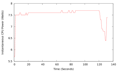
Figure 4: CPU power vs. time for the MC kernel

Figure 4 shows the power versus time plot for a standalone execution of the MC kernel. The BT execution plot is similar. The profile of instantaneous power versus time follows a very sharp trapezoidal shape: the CPU is fully utilized during execution and there are no periods of inactivity. This is a common feature with other numerically intensive HPC applications. It means that the measured average power is a representative measure of energy consumption throughout kernel execution.

In each experiment with multiple cores or nodes, we measure the worst execution time across all cores and use it as the elapsed time for all pricings.

6 Experiments and Results

We conducted two sets of experiments, one set where we executed the kernels in standalone mode and a second set where we executed the kernels in production mode, where each kernel is iterated to converge to an acceptable solution from a market perspective. We discuss the standalone kernel experiments and our findings in this section and the production experiments in the Section 7.

6.1 Kernel Experiments

Stock price data was recorded for a full session of a normal trading day in July 2014 and subsequently used to perform all experiments. By normal we mean that no significant initial public offerings (IPOs) or other skewed trading patterns took place on the market that day. We compiled and executed our OptionPricer on our laboratory servers and configured the installation to compute prices using MC and BT models for the 617 option contracts defined on the Facebook stock at the time. Each instance of the OptionPricer used as many compute threads as needed to fully subscribe the CPUs on all platforms.

Both the MC and the BT models are numerical approximations to the Black-Scholes analytical model, converging to this value as the number of iterations or steps $N$ approaches infinity. We selected three values of N for the MC computation 0.5M, 1M, 2M confirming that the relative error with respect to the Black-Scholes result decreased progressively to less than 0.1%. We found that to achieve comparable results with the BT model required N equal to 4000, 5000 and 7000 respectively. Fixing these values for $N$ in all simulations allows more insightful comparison of metrics across models.

For all experiments reported here, we replayed the collected data onto UDP multicast channels in our lab using tcpreplay. This enabled us to conduct the required kernel experiments. A single price update for one stock is pushed onto the multicast channel where it is read by each instance of the OptionPricer. All defined option contracts for that stock are then computed. Typically there are only a few hundred contracts open for one stock, meaning that these experiments are relatively short to run. These experiments allow precise investigation of the J/Option and Time/option metrics.

In our first set of experiments we investigated the effect of performance and powersave modes on energy consumption. Tables 2 , 3 and 4 (in the Appendix) show average power, compute time and and energy per option for each platform, executing the MC 1M and BT 5000 kernels and measuring the PRE-VRM power. Comparing the J/Opt values between performance and powersave modes, shows that performance mode is more energy efficient on all platforms and in both kernels. This is because computation latency under powersave execution increases disproportionately to power savings.

Specifically, on the Intel Sandy Bridge server, the PRE-VRM power consumption in powersave mode is about 2/3 of that in performance mode one, while energy is consistently worse. By contrast, computation latency doubles, thus negating any power savings. Note that in powersave mode the Intel CPU runs at 1.2 GHz, which is less than half of the performance mode frequency. This directly translates to more than a twofold increase in latency.

Considering the Viridis server numbers (Table 2), the increase in J/Option in powersave mode is even more pronounced. Powersave power consumption is again a little less than 2/3 of the power consumption in performance mode, but computation latency surprisingly increases by an order of magnitude. The Viridis powersave frequency (200 MHz) is 1/7 of the performance mode frequency (1.4 GHz). Apparently this does not translate to proportional power savings, because the ARM SoC includes several components which are not controllable through the DVFS interface.

The powersave mode measurements for all configurations of different platforms show a similar trend to different scales, viz. the powersave mode is not as energy efficient as the performance mode. Having observed this trend, all the results shown in the rest of this paper are in performance mode unless explicitly stated.

6.2 Other Findings

In this section we report on additional findings based on our kernel experiments. Kernels are run using different vectorization approaches, described in Section 4. To recap, we use the label NOVECT when the kernel code is not vectorized and AUTOVECT when we set the compiler flags to perform automatic vectorization. Moreover, we denote manual vectorization by referring to the specific instruction set and bit-width for each platform, e.g., NEON128 for the ARM cores. When manual vectorization uses compiler intrinsics instead of assembly, we denote this as INTRINSICS_xxx, e.g., INTRINSICS_NEON128, or as INTR-xxx for brevity.

(a) Viridis(1x4x1)

Figure 5: The cost of non-native transcedental operations on Viridis(1x4x1)

6.2.1 Support for transcendental functions

As discussed in Section 3, the MC kernel depends heavily on the calculation of transcendental functions, specifically the exponential. By contrast, the BT kernel spends most of the computation on floating point additions and multiplications. Additionally, Viridis ARM cores do not support native execution of exponentials while Intel platforms use native hardware for transcendental functions. Figure 5 illustrates the effect of transcendental function support on S/Opt and J/Opt metrics for Viridis, contrasting the MC and BT kernels.

One can easily notice this by capturing the difference between MC and BT algorithms on Viridis, which is an order of magnitude, while the same difference is much less on Intel’s Sandy Bridge (single node numbers in Tables 2, 3) and on Xeon Phi (Table 4).

6.2.2 Powersave governor mode

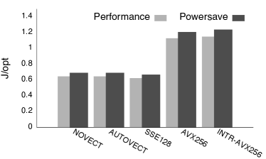
(a) MC Sandy Bridge (1x8x1)

(b) MC Sandy Bridge (2x8x1)

(c) BT Sandy Bridge (1x8x1)

(d) BT Sandy Bridge (2x8x1)

Figure 6: Power and energy efficiency on Sandy Bridge platforms for all kernels

Figure 7: Power and energy efficiency on Viridis(16x4x1) for the BT kernel

As previously discussed and mentioned here for completeness, performance mode is more energy efficient than powersave mode, despite the latter having a lower voltage-frequency setting. Figures 6 and  7 illustrate this result. Although power consumption is reduced significantly in powersave mode, the energy consumption increases for both Viridis and Sandy Bridge, using any vectorization method. Notably, J/Opt for Viridis is up to an order of magnitude less in performance mode than powersave mode while on Sandy Bridge the difference between them is much less. The reduction in power due to powersave mode is lost due to prolonged execution time and results in similar or higher energy consumption than performance mode. It is worth noting that vectorization in powersave mode recovers some of the lost performance, thus the J/Opt difference between the two modes shrinks. Comparing the J/Opt numbers for Xeon Phi in powersave and performance modes (Table 4), yields inconclusive results on the energy efficiency of the two modes. We are still investigating these results.

6.2.3 Vectorization Techniques

The BT and the MC algorithms perform better using intrinsics-based vectorization, than manual vectorization or autovectorization. This is because the compiler is able to do vectorization-neutral optimizations within code written using intrinsics while it cannot do so when we do manual vectorization through assembly. On all platforms, vectorization on the BT kernel lowers execution time proportionally but not linearly to the vector unit bit-width. This is because there is a small but still computationally significant part of the BT kernel which is not vectorizable. By contrast, the MC kernel gains little to nothing from vectorization due to the algorithmic reasons discussed earlier. On all platforms autovectorization seems to have a marginal effect (Tables 2, 3,  4), indicating inability of the compiler to break dependencies that prevent vectorization. The one notable exception is the vectorization of the BT algorithm by the ICC compiler on the Xeon Phi, which is nearly as effective as manual vectorization.

For Intel and Viridis, vectorization has little effect on power consumption, increasing it slightly in some cases. An interesting observation, which we are still investigating, is that vectorization on Phi actually reduces power consumption, see Table 4.

7 Fair Comparison of Servers and Microservers

In this section we are using our workload-specific and platform-independent metrics to directly compare our three server platforms. We refer to results provided in detail in Table 1. More detailed results are provided in Tables 2,  3, and  4 in the appendices. We perform comparisons using the vectorized or non-vectorized version of each kernel that achieves the fastest time per option priced on each platform. The fastest version of each kernel is also the least energy consuming version, with one exception, the MC kernel with 1 million iterations, executed on two Sandy Bridge sockets, where the SSE128 vectorized version consumes less energy than the autovectorized version, albeit being slightly slower. We report results from three sets of experiments with each kernel on each platform, where we vary the number of iterations in each kernel, reflecting different margins of error from the ideal analytical (Black Scholes) pricing solution for each kernel, which can be traded for execution speed in realistic market scenarios. We also report PRE-VRM power measurements on all platforms.

7.1 Monte Carlo Pricing

A single Viridis microsever underperforms a single Sandy Bridge socket in the MC kernel by one order of magnitude, with both running in performance mode. While this result can be traced to the many microarchitectural differences between the two platforms, our experiments suggest that the lack of efficient hardware implementation of transcendental functions on the ARM Cortex A9 processors is the critical culprit. That said, the Sandy Bridge socket expends almost six times as much power as the single microserver.

Taking the MC kernel with one million iterations as an example, we observe that counterbalancing low performance with low lower consumption yields a modest 18% energy loss to price a single option on Viridis. Notably, scaling out the Viridis microservers achieves a near ideal fifteen-fold speedup in time per option priced, with sustained energy consumed per option, as power also scales linearly to the number of microserver nodes. Scaling out from one to two Sandy Bridge sockets yields a non-ideal speedup of 1.63, while power consumption doubles. This narrows the gap in energy consumed per option to under 3% between the Sandy Bridge (better) and the Viridis (worse), the latter with scale out implemented. Sixteen ARM microserver nodes actually outperform two Sandy Bridge sockets in time per option, but incur an additional power tax of approximately 15 Watts.

Running the kernel with more or less than a million iterations indicates similar performance and energy-efficiency trends. The gap in energy per option priced between the Viridis microservers and the Sandy Bridge in scale out setup is a marginal 1.4%.

Table 1: Fastest S/Opt profiles for standalone kernel experiments

Kernel and	N	VEC TYPE	PRE-VRM	S/Opt	J/Opt
Platform		$\bar{P}$(W)
MC Viridis(1x4x1)	0.5M	INTRINSICS_NEON128	7.137	0.053298	0.380382
	1.0M	NEON128	7.258	0.105496	0.765691
	2.0M	NEON128	7.354	0.210560	1.548440
MC Viridis(16x4x1)	0.5M	NEON128	101.930	0.003761	0.383398
	1.0M	INTRINSICS_NEON128	102.680	0.007205	0.739765
	2.0M	NEON128	103.100	0.014316	1.476006
MC Intel(1x8x1)	0.5M	AUTOVECT	44.899	0.007138	0.320485
	1.0M	SSE128	44.852	0.013896	0.623238
	2.0M	SSE128	45.078	0.027672	1.247364
MC Intel(2x8x1)	0.5M	SSE128	87.814	0.004331	0.379259
	1.0M	NOVECT	90.999	0.008274	0.753282
	2.0M	AUTOVECT	96.691	0.016213	1.568116
MC Xeon Phi(1x1x1)	0.5M	KNC512	22.468	0.237212	5.329578
	1.0M	INTRINSICS_KNC512	22.510	0.473741	10.663713
	2.0M	NOVECT	22.852	0.947407	21.650439
MC Xeon Phi(1x60x1)	0.5M	KNC512	48.690	0.004589	0.223363
	1.0M	AUTOVECT	52.022	0.008925	0.464319
	2.0M	AUTOVECT	54.065	0.017400	0.940726
MC Xeon Phi(1x60x2)	0.5M	NOVECT	51.821	0.003582	0.185607
	1.0M	NOVECT	55.246	0.006720	0.371162
	2.0M	NOVECT	57.632	0.012860	0.741166
MC Xeon Phi(1x60x4)	0.5M	NOVECT	55.087	0.002967	0.163309
	1.0M	NOVECT	59.288	0.005348	0.317089
	2.0M	NOVECT	62.804	0.010188	0.639805
BT Viridis(1x4x1)	4000	NEON128	6.246	0.007143	0.044611
	5000	NEON128	6.317	0.011250	0.071070
	7000	INTRINSICS_NEON128	7.063	0.022279	0.157352
BT Viridis(16x4x1)	4000	NEON128	93.017	0.000649	0.060332
	5000	NEON128	93.783	0.000973	0.091239
	7000	INTRINSICS_NEON128	98.650	0.001702	0.167785
BT Intel(1x8x1)	4000	INITRINSICS_AVX256	40.494	0.001302	0.052729
	5000	INITRINSICS_AVX256	45.754	0.002222	0.101594
	7000	AVX256	48.642	0.005192	0.252550
BT Intel(2x8x1)	4000	AVX256	86.159	0.000710	0.060584
	5000	INITRINSICS_AVX256	80.621	0.001464	0.118039
	7000	INITRINSICS_AVX256	95.177	0.003192	0.303158
BT Xeon Phi(1x1x1)	4000	AUTOVECT	23.351	0.010955	0.255816
	5000	INTRINSICS_KNC512	22.758	0.017146	0.390209
	7000	AUTOVECT	23.012	0.033172	0.763351
BT Xeon Phi(1x60x1)	4000	INTRINSICS_KNC512	23.833	0.000387	0.009229
	5000	INTRINSICS_KNC512	25.417	0.000617	0.015824
	7000	KNC512	29.000	0.000745	0.021609
BT Xeon Phi(1x60x2)	4000	INTRINSICS_KNC512	26.583	0.000401	0.010666
	5000	KNC512	29.861	0.000466	0.013968
	7000	KNC512	39.238	0.000731	0.028691
BT Xeon Phi(1x60x4)	4000	INTRINSICS_KNC512	24.167	0.000544	0.013149
	5000	AUTOVECT	26.389	0.000586	0.015522
	7000	INTRINSICS_KNC512	30.917	0.000891	0.027531

The Xeon Phi server consumes more than two times less energy per option in the Monte Carlo kernel compared to both Viridis and the Sandy Bridge server. Notably, the Xeon Phi does so without employing vectorization and with a significant boost in performance and energy-efficiency from Hyperthreading on each core. Taking the case with one million iterations as an example (other cases behave similarly), the Phi with all cores and threads activated provides a seemingly modest 34% performance improvement over the Viridis (more compared to Sandy Bridge) but offers a significantly better power-efficiency proposition with 60 cores and 240 threads burning under 60 Watt, when the scaled out Viridis microservers offers 64 cores at just over 100 Watt. Note that a single Phi core is two to three times slower than one Sandy Bridge core and marginally slower with one ARM Cortex A9 core in terms of performance.

Conclusion:

For a real-time option pricing workload using Monte Carlo methods, the Xeon Phi is the best performing and most energy-efficient option. A scaled out ARM microserver is in par with a heavyweight Sandy Bridge server in terms of energy cost, but can provide higher performance.

7.2 Binomial Tree

The lesser dependence of the BT kernel on transcendental functions becomes apparent from single-node experiments: A single microserver is 5.5 times slower than a single Sandy Bridge socket (vis. 7.5 times in the MC kernel). A single Phi core is 2.5 times faster than a single ARM Cortex A9 core thanks to the higher quality vectorization of the BT kernel on the Phi and the more powerful SIMD set available on the Phi, compared to the A9.

Scaling out the microserver yields dramatically lower energy consumption per option priced than the Sandy Bridge server. For example, running the BT kernel with 7000 iterations consumes 81% less Joules per option on microservers compared to the Sandy Bridge. Sixteen microservers also outperform two Sandy Bridge sockets by as much as 46%. Note that in scale out mode the power consumption of both the Viridis and the Sandy Bridge servers are comparable. This surprising result -considering the difference in single-core performance between the two platforms- can be explained by workload effects. The Viridis server offers the fact that the BT model has two imbalanced computational phases. The setup phase has linear complexity and involves transcendental functions, which are faster on Intel hardware. The second phase is the tree scanning phase, which has quadratic complexity, and uses only floating point addition and multiplication operations. These operations execute natively on both platforms. While the Sandy Bridge has an advantage over the ARM on the initialization phase, this advantage diminishes in the computation phase and is marginalized as the number of iterations of the BT kernel grows.

The Xeon Phi offers once again an excellent power-efficiency proposition. Compared to the Viridis microservers in scale out setup, the Phi achieves twice the performance, at a third of the power budget, for a sixfold reduction of energy per option priced.

Conclusion:

For a real-time option pricing workload using Binomial Tree methods, the Xeon Phi is the best performing and most energy-efficient option. A scaled out ARM microserver is significantly faster and more energy-efficient than an equivalent, from a power perspective, Sandy Bridge server.

7.3 QoS Discussion

In a live market situation the question arises whether option pricing can keep pace with the rate of arrival of new stock prices. We use the QoS metric defined in Section 5 to consider the implications of dynamic deadlines set by market conditions on the option pricing workload. We define an iso-QoS comparison method, where we compare the performance, power and energy of different platforms, with setups that achieve the same QoS for a given workload. One can conduct similar exercises using iso-metrics that equate power, performance, energy consumption, or combined efficiency metrics.

Figure 8: All-or-nothing pricing vs. stock price update intervals

A new stock price arrival triggers a computation of all available option contracts. The most stringent QoS requirement is “all-or-nothing”: the pricing of all options must complete before another stock price update, otherwise any computation performed before the deadline is discarded, having wasted time and energy.

Indicatively, Figure 8 shows the percentage of successful all-or-nothing option pricing computations as a function of the cumulative number of price updates, sorted into bins of 0.25 second intervals. The data for our experiments are taken from a trading session of 6.5 hours where 10,156 price updates occurred for the Facebook stock, producing the cumulative profile shown in the figure.

Nonetheless, there are trading scenarios where the financial user does not require this all-or-nothing approach. For example a user may prefer to price a subset of options, such as short-term or long-term expiring ones, for which there is financial interest. Moreover, the all-or-nothing approach disregards the fact that some options were indeed correctly priced and they can be used for trading. For these reasons we relax this requirement and defined our QoS metric as the percentage of successfully priced option contracts over the total number of option contract pricings.

Figure 8 shows the QoS profile of the Viridis and Sandy Bridge platforms with two scenarios of Monte Carlo (half a million iterations) and Binomial Tree (4000 iterations). Both platforms run in performance mode and are scaled to the maximum number of cores available. The figure shows the performance gap between options pricing on the two platforms. The microserver is able to price all options using Monte Carlo slightly faster ($[2.25-2.50]$ seconds time bin), while the Sandy Bridge is slower ($[2.50-2.75]$ seconds bin) but both platforms exhibit low QoS (13.5% and 12.5% respectively), which may be unacceptable for an end user. On the other hand, both platforms exhibit 100% QoS with the Binomial Tree kernel, where the Viridis microservers also reduce total energy consumption by as much as 55%.

8 Related Work

Recent work related to ours explores the performance and power consumption of low-power ARM processor models that attempt to enter the server [4, 5] and HPC markets [3]. Our study targets a different domain, real-time financial analytics, and provides a comparison between fully integrated ARM-based microservers in scale-out configurations, against high-end Intel servers. We also provide further insight on the viability of the ARM ecosystem for datacenters and high-performance computing, using new platform-independent metrics and a comprehensive method to ensure fair comparison. The work of Blem et al [21] is perhaps the closest to ours. It explores the performance and power consumption of several ARM and Intel processors. However, their study focuses on the energy and performance implications of ISA choices on the different processors, rather than the use of the processors at scale or their deployment in specific application domains. Anwar et al [22] study microserver performance with Hadoop workloads. Our work advances the state of knowledge in microservers, by exploring the performance and energy implications of scaling their resources up and out and by placing microservers on a fair comparison basis against both general-purpose servers and accelerators targeting the HPC market.

Also related to our contribution is work that measures the energy-efficiency of specific algorithms and numerically intensive kernels. Alonso et al [23] model the power and energy of a specific task-parallel implementation of Cholesky factorization. Dongarra et al [24] explore the energy footprint of dense numerical linear algebra libraries on multicore systems. Korthikanti et al  [25] analyzed the energy scalability of parallel algorithms on shared-memory multicore architectures, focusing on the sensitivity of the the algorithms to the critical path length, the power consumption of instruction execution and the power consumption of memory accesses. Within the European PRACE project, a performance specific to 2D stencil applications on multi-core parallel machines was derived [26]. Kozin [27] analyzed the execution of several computational chemistry codes on Nehalem servers and on a heterogeneous system composed of one Nehalem server and one Tesla GPU system. They reported that idle power was a significant component of overall power consumption. Our work differs in that it explores a dynamic workload with real-time execution requirements and a mixture of event-driven and data parallelism.

9 Conclusions

In this paper we have presented a fair methodology for comparing server platforms for real-time financial analytics. Our methodology considers performance, energy-efficiency, and QoS impact on energy consumption, hence cost of provisioning these services. We have based our methodology on workload-specific but platform-independent metrics, which facilitated direct performance and cost comparisons. These comparisons will benefit directly datacenter operators during hardware procurement and provisioning exercises, but also developers of financial services during exercises to reduce service cost while sustaining competitive performance and QoS in their products. Notably, our study used real stock market streaming data and captured the dynamic, event-driven nature of real-time financial analytics workloads.

Our results show that microservers based on ARM processors are viable contenders to state-of-the-art general-purpose servers. Scaled out microserver configurations achieve similar or better performance and similar or improved energy-efficiency under a fixed power budget. However, microservers can not match densely packaged many-core accelerators, such as the Xeon Phi. The introduction of such computational accelerators within the power and area constraints of microservers is thus a promising area of further investigation. Extending our methodology and metrics to heterogeneous platforms is also appropriate given the increasing presence of such platforms in datacenters. providing the same quality of service. One further open area for future research is the exact error behavior of the MC and BT models in response to reducing their energy consumption by reducing their number of iterations.

Acknowledgments

The work was supported by the European Commission under its Seventh Framework Programme, grant number 610509 (NanoStreams). This work was also supported by the UK Engineering and Physical Sciences Research Council, under grant agreements EP/K017594/1, EP/L000055/1 and EP/L004232/1.

Appendix A Appendix

Table 2: Viridis S/Opt and J/Opt metrics, using PRE-VRM power

	Performance			Powersave
	$\bar{P}(W)$	S/Opt	J/Opt	$\bar{P}(W)$	S/Opt	J/Opt
Viridis(1x4x1)
MC 1M NOVECT	7.19922	0.11472	0.82590	4.33896	0.90668	3.93405
AUTOVECT	7.27235	0.11522	0.83793	4.34735	0.94811	4.12176
NEON128	7.25806	0.10550	0.76570	4.31920	0.83421	3.60314
INTRINSICS_NEON128	7.23137	0.10810	0.78171	4.32488	0.84103	3.63736
BT 5000 NOVECT	7.44259	0.01584	0.11786	4.28633	0.11307	0.48467
AUTOVECT	7.39630	0.01580	0.11687	4.26875	0.11324	0.48340
NEON128	6.31710	0.01125	0.07107	4.20724	0.08048	0.33858
INTRINSICS_NEON128	7.11229	0.01270	0.09032	4.46305	0.10792	0.48163
Viridis(16x4x1)
MC 1M NOVECT	101.00667	0.00820	0.82863	63.17333	0.06537	4.12953
AUTOVECT	102.50000	0.00817	0.83756	62.41000	0.07180	4.48118
NEON128	102.93333	0.00731	0.75209	62.57000	0.06431	4.02363
INTRINSICS_NEON128	102.68000	0.00721	0.73976	85.13000	0.02644	2.25080
BT 5000 NOVECT	103.14333	0.00130	0.13379	63.22667	0.00773	0.48885
AUTOVECT	103.83500	0.00130	0.13469	61.58333	0.00790	0.48618
NEON128	93.78333	0.00097	0.09124	64.25000	0.00400	0.25707
INTRINSICS_NEON128	93.72333	0.00097	0.09118	68.75667	0.00249	0.17106

Table 3: Intel Sandy Bridge S/Opt and J/Opt metrics, using PRE-VRM power

	Performance			Powersave
	$\bar{P}(W)$	S/Opt	J/Opt	$\bar{P}(W)$	S/Opt	J/Opt
Intel(1x8x1)
MC 1M NOVECT	45.04794	0.014325	0.645297	28.689189	0.024103	0.691485
AUTOVECT	45.269019	0.014271	0.646025	28.692122	0.024109	0.69175
SSE128	44.85186	0.013896	0.623248	28.579088	0.02335	0.667322
AVX256	45.26695	0.024919	1.128025	28.721541	0.042054	1.207863
INTRINSICS_AVX256	45.441663	0.0253	1.149656	28.739781	0.043073	1.237895
BT 5000 NOVECT	43.27172	0.00584	0.252717	27.78212	0.009733	0.270402
AUTOVECT	43.293392	0.005838	0.252739	27.798964	0.009732	0.27053
SSE128	44.113263	0.003894	0.171773	28.989414	0.006164	0.178696
AVX256	45.450668	0.002275	0.1034	30.116217	0.00357	0.107502
INTRINSICS_AVX256	45.754212	0.002222	0.101684	29.627705	0.003568	0.10572
Intel(2x8x1)
MC 1M NOVECT	90.999305	0.008274	0.7529	57.925196	0.01482	0.858431
AUTOVECT	90.048869	0.008453	0.761147	54.843581	0.014646	0.803252
SSE128	84.694158	0.008493	0.719341	60.652193	0.012971	0.786716
AVX256	88.619245	0.014214	1.259592	57.493955	0.024968	1.435523
INTRINSICS_AVX256	89.048027	0.015029	1.338341	57.128128	0.026699	1.525274
BT 5000 NOVECT	85.380722	0.00364	0.310779	55.24572	0.006228	0.344074
AUTOVECT	81.84787	0.00368	0.301215	69.158565	0.005629	0.389319
SSE128	79.325308	0.002655	0.210598	55.302365	0.003908	0.216115
AVX256	79.732068	0.001525	0.121553	57.545024	0.002342	0.134773
INTRINSICS_AVX256	80.620701	0.001464	0.118034	59.139075	0.002166	0.128069

Table 4: Xeon Phi Joules, S/Opt and J/Opt metrics using PRE-VRM power

	Performance			Powersave
	$\bar{P}(W)$	S/Opt	J/Opt	$\bar{P}(W)$	S/Opt	J/Opt
Xeon Phi(1x1x1)
MC 1M NOVECT	22.97195	0.4742	10.89323	17.80396	0.59137	10.52876
AUTOVECT	22.4946	0.47401	10.66273	16.3638	0.59208	9.68871
KNC512	22.53165	0.47481	10.69822	16.64192	0.59276	9.86468
INTRINSICS_KNC512	22.50958	0.47374	10.66371	16.36761	0.59237	9.69560
BT 5000 NOVECT	22.99814	0.10305	2.36986	17.43763	0.12869	2.24396
AUTOVECT	23.09841	0.01720	0.39733	17.78937	0.02139	0.38046
KNC512	22.71311	0.01716	0.38979	17.87900	0.02139	0.38242
INTRINSICS_KNC512	22.75758	0.01715	0.39021	17.87283	0.02139	0.38232
Xeon Phi(1x60x1)
MC 1M NOVECT	49.44860	0.00919	0.45453	41.95386	0.01149	0.48213
AUTOVECT	52.02175	0.00893	0.46432	42.38235	0.01154	0.48888
KNC512	51.94204	0.00893	0.46403	42.22966	0.01154	0.48716
INTRINSICS_KNC512	51.52656	0.00913	0.47059	42.82180	0.01118	0.47882
BT 5000 NOVECT	47.44445	0.00208	0.09861	40.55693	0.00254	0.10293
AUTOVECT	26.08333	0.00073	0.01896	20.16667	0.00078	0.01570
KNC512	25.91667	0.00062	0.01603	19.94445	0.00074	0.01479
INTRINSICS_KNC512	25.41667	0.00062	0.01568	20.58333	0.00077	0.01574
Xeon Phi(1x60x2)
MC 1M NOVECT	55.24644	0.00672	0.37128	47.19607	0.00811	0.38260
AUTOVECT	57.22312	0.00678	0.38811	46.85469	0.00827	0.38760
KNC512	58.64738	0.00675	0.39592	47.04584	0.00814	0.38304
INTRINSICS_KNC512	57.09140	0.00715	0.40821	46.20823	0.00849	0.39231
BT 5000 NOVECT	50.37038	0.00177	0.08908	44.01588	0.00213	0.09375
AUTOVECT	30.80159	0.00062	0.01923	26.54167	0.00076	0.02013
KNC512	29.86111	0.00047	0.01392	27.87500	0.00078	0.02176
INTRINSICS_KNC512	28.47619	0.00056	0.01590	27.57937	0.00073	0.02014
Xeon Phi(1x60x4)
MC 1M NOVECT	59.28792	0.00535	0.31709	49.90982	0.00674	0.33656
AUTOVECT	59.76438	0.00573	0.34251	50.66874	0.00701	0.35528
KNC512	61.00413	0.00575	0.35089	51.90346	0.00672	0.34882
INTRINSICS_KNC512	62.66650	0.00554	0.34707	51.63727	0.00673	0.34761
BT 5000 NOVECT	47.09524	0.00148	0.06985	41.64147	0.00160	0.06645
AUTOVECT	26.38889	0.00059	0.01545	20.52778	0.00076	0.01554
KNC512	26.11667	0.00083	0.02171	20.66667	0.00085	0.01755
INTRINSICS_KNC512	25.33333	0.00060	0.01521	21.05556	0.00090	0.01885

References

- [1] Gillan CJ, Nikolopoulos DS, Georgakoudis G, Faloon R, Tzenakis G, Spence I. On the viability of microservers for financial analytics. Proceedings of the 7th Workshop on High Performance Computational Finance, WHPCF ’14, IEEE Press: Piscataway, NJ, USA, 2014; 29–36, doi:10.1109/WHPCF.2014.11. URL http://dx.doi.org/10.1109/WHPCF.2014.11.
- [2] Novakovic S, Daglis A, Bugnion E, Falsafi B, Grot B. Scale-out numa. Proceedings of the 19th International Conference on Architectural Support for Programming Languages and Operating Systems, ASPLOS ’14, 2014; 3–18, doi:10.1145/2541940.2541965. URL http://doi.acm.org/10.1145/2541940.2541965.
- [3] Rajovic N, Carpenter PM, Gelado I, Puzovic N, Ramirez A, Valero M. Supercomputing with commodity cpus: Are mobile socs ready for hpc? Proceedings of the International Conference on High Performance Computing, Networking, Storage and Analysis, SC ’13, 2013; 40:1–40:12, doi:10.1145/2503210.2503281. URL http://doi.acm.org/10.1145/2503210.2503281.
- [4] Tudor BM, Teo YM. On understanding the energy consumption of arm-based multicore servers. Proceedings of the ACM SIGMETRICS/International Conference on Measurement and Modeling of Computer Systems, SIGMETRICS ’13, 2013; 267–278, doi:10.1145/2465529.2465553. URL http://doi.acm.org/10.1145/2465529.2465553.
- [5] Ou Z, Pang B, Deng Y, Nurminen JK, Yla-Jaaski A, Hui P. Energy- and cost-efficiency analysis of arm-based clusters. Proceedings of the 2012 12th IEEE/ACM International Symposium on Cluster, Cloud and Grid Computing (Ccgrid 2012), CCGRID ’12, 2012; 115–123, doi:10.1109/CCGrid.2012.84. URL http://dx.doi.org/10.1109/CCGrid.2012.84.
- [6] Allen R, Johnson S. Compiling c for vectorization, parallelization, and inline expansion. SIGPLAN Not. Jun 1988; 23(7):241–249, doi:10.1145/960116.54014. URL http://doi.acm.org/10.1145/960116.54014.
- [7] S L, S A. Exploiting superword level parallelism with multimedia instruction sets. Proceedings of the ACM SIGPLAN conference on Programming language design and implementation, vol. 35, 2000; 145–156.
- [8] Shin J HMW, J C. Superword-level parallelism in the presence of control flow. Proceedings of the international symposium on Code generation and optimization, 2005; 165–175.
- [9] Shin J. Introducing control flow into vectorized code. Proceedings of the 16th International Conference on Parallel Architecture and Compilation Techniques, 2007; 280–291.
- [10] JV Mullan CG, Fusco V. Optimizing the parallel implementation of a finite difference time domain code on a multi-user network of workstations. APPLIED COMPUTATIONAL ELECTROMAGNETICS SOCIETY JOURNAL SPECIAL ISSUE ON COMPUTATIONAL ELECTROMAGNETICS AND HIGH-PERFORMANCE COMPUTING 1998; 13.
- [11] Gillan CJ, Fusco VF. High performance distributed fdtd electromagnetic field computation for electronic circuit design. High-Performance Computing 1999; :569–574.
- [12] Black F, Scholes M. The valuation of option contracts and a test of market efficiency. J. Finance 1972; 27:399–418.
- [13] Black F, Scholes M. The pricing of options and corporate liabilities. J. Political Econonomy 1973; 81:637–54.
- [14] P Boyle MB, Glasserman P. Monte carlo methods for security pricing. J. Econ. Dynamics and Control 1997; 21:1267–321.
- [15] Linz P. Accurate floating point summation. Numerical mathematics 1970; 13:361–2.
- [16] Higham NJ. The accuracy of floating point summation. SIAM J. Sci. Comput 1993; 14:783–799.
- [17] Matsumoto M, Nishimura T. Mersenne twister: a 623-dimensionally equidistributed uniform pseudo-random number generator. ACM Transactions on Modeling and Computer Simulation 1998; 8:3–30.
- [18] J C Cox SAR, Rubinstein M. Option pricing: A simplified approach. Journal of Financial Economics 1979; 7:779.
- [19] Moshier SL. Cephes math library 2000. See http://www.moshier.net.
- [20] Manousakis I, Nikolopoulos DS. Btl: A framework for measuring and modeling energy in memory hierarchies. 2012 IEEE 24th International Symposium on Computer Architecture and High Performance Computing, 2012; 139–46.
- [21] Blem E, Menon J, Sankaralingam K. Power struggles: Revisiting the risc vs. cisc debate on contemporary arm and x86 architectures. Proceedings of the 2013 IEEE 19th International Symposium on High Performance Computer Architecture (HPCA), HPCA ’13, 2013; 1–12, doi:10.1109/HPCA.2013.6522302. URL http://dx.doi.org/10.1109/HPCA.2013.6522302.
- [22] Anwar A KK, AR B. On the use of microservers in supporting hadoop applications. Cluster Computing (CLUST), 2014 International Conference on, 2014; 66–74.
- [23] Alonso P, Dolz MF, Mayo R, Quintana-Ortí ES. Modeling power and energy of the task-parallel cholesky factorization on multicore processors. Computer Science - R&D 2014; 29(2):105–112.
- [24] Dongarra J, Ltaief H, Luszczek P, Weaver V. Energy footprint of advanced dense numerical linear algebra using tile algorithms on multicore architectures. Cloud and Green Computing (CGC), 2012 Second International Conference on, 2012; 274–281, doi:10.1109/CGC.2012.113.
- [25] Korthikanti VA, Agha G. Towards optimizing energy costs of algorithms for shared memory architectures. Proceedings of the 22nd Annual ACM Symposium on Parallelism in Algorithms and Architectures, Thira, Santorini, Greece, 2010; 157–165.
- [26] Hou Z, Perez C. Auto-tuning 2d stencil applications on multi-core parallel machines. PRACE Whitepapers, 2012. URL http://www.prace-ri.eu/IMG/pdf/wp52_auto-tuning_2d_stencil_applications_on_multi-core_parallel_machines.pdf.
- [27] Kozin I. Power efficiency in hpc. The 22nd Daresbury Machine Evaluation Workshop, 2011. URL http://www.cse.scitech.ac.uk/events/mew22/programme.html.