Lifting for Blind Deconvolution in Random Mask Imaging: Identifiability and Convex Relaxation

Abstract

In this paper we analyze the blind deconvolution of an image and an unknown blur in a coded imaging system. The measurements consist of subsampled convolution of an unknown blurring kernel with multiple random binary modulations (coded masks) of the image. To perform the deconvolution, we consider a standard lifting of the image and the blurring kernel that transforms the measurements into a set of linear equations of the matrix formed by their outer product. Any rank-one solution to this system of equation provides a valid pair of an image and a blur.

We first express the necessary and sufficient conditions for the uniqueness of a rank-one solution under some additional assumptions (uniform subsampling and no limit on the number of coded masks). These conditions are special case of a previously established result regarding identifiability in the matrix completion problem. We also characterize a low-dimensional subspace model for the blur kernel that is sufficient to guarantee identifiability, including the interesting instance of “bandpass” blur kernels.

Next, assuming the bandpass model for the blur kernel, we show that the image and the blur kernel can be found using nuclear norm minimization. Our main results show that recovery is achieved (with high probability) when the number of masks is on the order of $\mu\log^{2}L\,\log\frac{Le}{\mu}\,\log\log\left(N+1\right)$ where $\mu$ is the coherence of the blur, $L$ is the dimension of the image, and $N$ is the number of measured samples per mask.

1 Introduction

The blind deconvolution problem has been encountered in many fields including astronomical, microscopic, and medical imaging, computational photography, and wireless communications. Many blind deconvolution techniques, that are mostly tailored for particular applications, have been proposed in these communities. These techniques can be divided into two categories based on their general formulation of the problem. The methods of the first category typically reduce the blind deconvolution problem to a regularized least squares problem without imposing stochastic models on either of the convolved signals. High computational cost and sensitivity to noise are the main challenges for these methods. The second category of blind deconvolution methods follow a Bayesian approach and consider prior distributions for either or both of the signals. An extensive review of the classic blind deconvolution methods in imaging can be found in [4]. A survey of the multichannel blind deconvolution methods used in communications can be found in [24] as well.

1.1 Contributions

In recent years, various imaging architectures have been proposed that are based on randomly coded apertures. For example, in [18], rapid switching of exposure of cameras in random patterns is leveraged for motion deblurring. Furthermore, in the “single-pixel-camera” [8] and compressive hyperspectral imaging systems [22, 13, 15, 17], randomly coded masks are utilized to radically reduce the cost associated with spatial or spectral sampling in traditional imaging systems. In this paper, we consider the blind deconvolution problem in a similar imaging architecture that relies on randomly coded masks. As illustrated in Figure 1, the considered imaging system first generates different modulated copies of the target image, each of which is then blurred by a fixed unknown filter (i.e., the blurring kernel), and finally subsampled by a relatively small number of sensors. Throughout the paper, we only consider a uniform subsampling operator in our model. This idealized subsampling operator corresponds to an array of single pixel sensors with uniform spacing. However, a broader class of subsampling schemes can be treated in a similar fashion. For example, a more realistic model for a single sensor is a weighted integrator of a few neighboring pixels. Spatially uniform subsampling with an array of these types of sensors can be reduced to the pointwise subsampling by absorbing the weight window into the blur filter. We believe that our analysis can be extended to even broader class of subsampling schemes, but we do not pursue these extensions in this paper.

As will be discussed in Section 3, in the absence of any model for the blurring kernel the subsampling operation renders the unique recovery of the image impossible, regardless of the number of measurements acquired. Intuitively, there are two competing requirements for the blurring kernel in the considered imaging system. First, it is necessary that the image is blurred and spread to the extent that the subsampling sensors do not miss any pixel of the image. As will be seen, this requirement can be satisfied by considering a subspace model for the blurring kernel. Second, the blurring should not be excessive, otherwise the sampling becomes inefficient as different sensors collect (nearly) identical measurements. As will be seen in Section 3.2, the severity of the blur can be quantified by the coherence of the blurring kernel. Specifically, our results show that the coherence critically affects the sufficient number of masks for successful reconstruction through convex optimization.

We first study identifiability of the problem without restricting the number of measurements. In Section 3.1, using the results of [11] for matrix completion we express a necessary and sufficient condition for identifiability which has a combinatorial nature. Often, optical models can provide us with some crude approximations of the blurring kernel that can be leveraged as prior information. For example, we can conveniently incorporate these prior information in a subspace model where the linear span of the available approximations is considered as the set of feasible blurring kernels. Our second and more concrete identifiability result is obtained by considering a low-dimensional subspace model for the blurring kernel. We show that the described blind deconvolution problem is identifiable, if the mentioned low-dimensional subspace obeys certain conditions. In particular, our results show that if the blurring kernel has a sufficiently narrow “bandwidth” then the desired condition holds and thus we can uniquely identify the image and the blurring kernel.

In the second part of our work, we show that, under a “bandpass” blur model, we can perform the blind deconvolution through lifting and nuclear norm minimization. This systematic approach applies not only to our blind deconvolution problem, but also to a variety of other bilinear inverse problems that involve unknown linear operators. The theoretical guarantees, which are explained in Section 3.2, rely on construction of a dual certificate for the nuclear norm minimization problem via the golfing scheme [9]. Furthermore, the concentration inequalities recently developed in the field of random matrix theory are frequently used throughout the derivations. Finally, while we state our results under the bandpass modelling of the filter, with some effort similar results can be established for the more general subspaces described by the identifiability sufficient conditions.

1.2 Related work

In [5], the PhaseLift method [7] is extended to address the phase retrieval problem in coded diffraction imaging, where the measurements have a more intricate structure. It is shown that the trace minimization (i.e., PhaseLift) can solve the phase retrieval problem, if the randomly coded masks follow certain “admissible” distributions and their number is poly-logarithmic in the ambient dimension. The use of coded masks in the phase retrieval problem of [5] is effectively similar to that in the blind deconvolution problem we address in this paper. However, the measurement model in this paper is different from that of [5].

In [1], a convex programming technique is proposed for blind deconvolution, where by lifting the signal and the filter to their outer product, the problem is cast as reconstruction of a rank-one matrix from a set of linear measurements. It is shown in [1] that the nuclear norm minimization can robustly and accurately recover the rank-one solution to the convolution equations. This blind deconvolution technique imposes certain low-dimensional subspace structures on the input and channel to reach a well-posed problem.

More recently, [23] has examined the problem of blind deconvolution in an imaging system similar to what considered in this paper. It is shown in [23] that one can recover the image and the blurring kernel through lifting and nuclear norm minimization, provided that the number of applied masks is greater that the coherence of the blurring kernel by a poly-logarithmic factor of the image length. The fact that we consider the effect of subsampling makes the imaging model considered in this paper more general than that of [23]. In the special case that subsampling is not applied, our problem reduces to that of [23]. In this regime, the sufficient number of masks obtained here and in [23] have similar growth order. Only for blurring kernels that have more uniform spectrum (i.e., have low coherence), our bounds can be slightly worse up to a double logarithmic factor of the image length. We believe that our bounds can be further improved using sharper inequalities throughout the derivations, but we do not attempt to find the optimal logarithmic factors.

1.3 Notation

Throughout this paper we use the following notation. Matrices and vectors are denoted by bold capital and small letters, respectively. A superscipt asterisk denotes the Hermitian transpose of matrices and vectors (e.g., $\boldsymbol{X}^{*}$, $\boldsymbol{x}^{*}$). More generally, the same symbol denotes the adjoint of linear operators (e.g., $\mathcal{A}^{*}$). Restriction of a matrix $\boldsymbol{X}$ to the columns enumerated by an index set $\mathsf{J}$ is denoted by $\boldsymbol{X}_{\mathsf{J}}$. For a vector $\boldsymbol{x}$, we write $\left.\boldsymbol{x}\right|_{\mathsf{J}}$ to denote its restriction to the entries indicated by the index set $\mathsf{J}$. Real and imaginary parts of complex variables are denoted by preceding symbols $\Re$ and $\Im$, respectively. Scalar functions applied to vectors or matrices act entrywise. Nullspace and range of linear operators are denoted by $\mathrm{null}\left(\cdot\right)$ and $\mathrm{range}\left(\cdot\right)$, respectively. Hadamard product (i.e., entrywise product) operation on two matrices or vectors is denoted by $\odot$ symbol. Entrywise conjugate of a matrix (or vector) is denoted by putting a bar above the variable (e.g., $\overline{\boldsymbol{X}}$ is the entrywise conjugate of $\boldsymbol{X}$). We frequently use the normalized Discrete Fourier Transform (DFT) matrix which is denoted by $\boldsymbol{F}$ whose size should be clear from the context. Furthermore, $\boldsymbol{F}_{n}$ is used to denote for the restriction of $\boldsymbol{F}$ to its first $n$ rows. Moreover, the $l$-th column of $\boldsymbol{F}^{*}$ is denoted by $\boldsymbol{f}_{l}$. The DFT of a vector is denoted by the same name with a hat sign atop (e.g., for $\boldsymbol{x}\in\mathbb{C}^{L}$, the DFT of $\boldsymbol{x}$ is denoted by $\widehat{\boldsymbol{x}}=\sqrt{L}\boldsymbol{F}\boldsymbol{x}$).The diagonal matrix whose diagonal entries form a vector $\boldsymbol{x}$ is denoted by $\boldsymbol{D}_{\boldsymbol{x}}$. Furthermore, the matrix of diagonal entries of a square matrix $\boldsymbol{X}$ is denoted by $\mathrm{diag}\left(\boldsymbol{X}\right)$. The vector norms $\left\|\cdot\right\|_{p}$ for $p\geq 1$ are the standard $\ell_{p}$-norms. The spectral norm, the Frobenius norm, and the nuclear norm are denoted by $\left\|\cdot\right\|$, $\left\|\cdot\right\|_{F}$, and $\left\|\cdot\right\|_{*}$, respectively. We find it convenient to use the expression $f\overset{\beta}{\gtrsim}g$ (or $f\overset{\beta}{\lesssim}g$) as a shorthand for inequalities of the form $f\geq c_{\beta}g$ (or $c_{\beta}f\leq g$), where $c_{\beta}>0$ is some absolute constant that depends only a parameter $\beta$. We drop the superscript in this notation whenever the constant factors do not depend on any parameter.

2 Problem setup

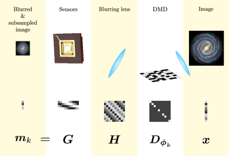
Fig. 1: Schematic of the masked imaging system. The reflection of the target image from a DMD with a random pattern is blurred by a lens and then subsampled by a few sensors. The result is one set of measurements that correspond to the chosen DMD pattern.

We consider a blind deconvolution problem in an imaging system depicted by Figure 1 that involves subsampling. To simplify the exposition, through out the paper we consider 1D blind deconvolution, but generalization to 2D models is straightforward. In our model, multiple binary masks $\boldsymbol{\phi}_{k}$ ($k=1,2,\dotsc,K$) are applied to an image represented by $\boldsymbol{x}\in\mathbb{R}^{L}$ one at a time by the means of a Digital Micromirror Device (DMD). The masked reflection of the image from the DMD is then blurred through a secondary lens represented by a filter $\boldsymbol{h}\in\mathbb{R}^{L}$. We model the action of the filter on its input by a circular convolution. The masked and blurred image is then subsampled using $N\leq L$ sensors. Mathematically, the described system can be represented by the equations

$$\boldsymbol{m}_{k} =\boldsymbol{G}\boldsymbol{H}\boldsymbol{D}_{\boldsymbol{\phi}_{k}}\boldsymbol{x},$$

where $\boldsymbol{H}$ is a circulant matrix whose first column is $\boldsymbol{h}$ which models the blurring lens, $\boldsymbol{G}$ is an $N\times L$ matrix representing the (linear) subsampling operator, and $\boldsymbol{m}_{k}$ is the $k$-th measurement, corresponding to the $k$-th mask $\boldsymbol{\phi}_{k}$. In this paper, we exclusively consider uniform pointwise subsampling as our subsampling operator $\boldsymbol{G}$. Note that the above equation for all of the measurements can be written compactly as

(1) $$\boldsymbol{M} =\boldsymbol{G}\boldsymbol{H}\boldsymbol{D}_{\boldsymbol{x}}\boldsymbol{\Phi},$$

where $\boldsymbol{\Phi}=\left[\begin{array}[]{cccc}\boldsymbol{\phi}_{1}&\boldsymbol{\phi}_{2}&\dotsm&\boldsymbol{\phi}_{K}\end{array}\right]$ is the matrix of masks and $\boldsymbol{M}=\left[\begin{array}[]{cccc}\boldsymbol{m}_{1}&\boldsymbol{m}_{2}&\dotsm&\boldsymbol{m}_{K}\end{array}\right]$ is the matrix of measurements.

Accurate estimates of the blurring kernel $\boldsymbol{h}$ might not be available in practice. For example, random vibrations of the lens and the subject relative to each other, turbulence of the propagation medium, or errors in measuring the focal length of the lens can preclude accurate estimation of the blur. Therefore, it is highly desirable to perform a blind deconvolution for reconstruction of both the image and the blurring kernel from the measurements of the form (1) up to the global scaling ambiguity.

Because $\boldsymbol{G}$ is in general a wide matrix, recovery of $\boldsymbol{h}$ and $\boldsymbol{x}$ (up to a scaling factor) can be ill-posed even with an unlimited number of masks. Therefore, it is worthwhile to study the identifiability of our inverse problem under the assumption $\boldsymbol{\Phi=\boldsymbol{I}}$. In Section 3.1, we elaborate on the conditions under which we can guarantee identifiability.

In Section 3.2 we introduce a convex program as a systematic method for the blind deconvolution. To analyze this method, we assume that the blurring kernel follows a “bandpass” model that was suggested by the sufficient identifiability conditions. In particular, in Section 3.2 we assume that $\boldsymbol{h}=\frac{1}{\sqrt{L}}\boldsymbol{F}_{N}\widehat{\boldsymbol{h}}$ is the blurring kernel for some $N$-dimensional vector $\widehat{\boldsymbol{h}}$. Furthermore, to have a realistic model of the system, we assume that the number of masks is limited and should be relatively small. While ideal binary masks are $\left\{0,1\right\}$-valued, for technical reasons we consider the elements of $\boldsymbol{\Phi}$ to be iid Rademacher random variables that take values in $\left\{\pm 1\right\}$ with equal probability. Note that this assumption is not unrealistic as the $\left\{0,1\right\}$-valued masks can be converted to $\left\{\pm 1\right\}$-valued masks by using an extra all-one mask.

3 Main results

3.1 Identifiability without measurement limitations

In this section we analyze the identifiability of the image and blurring kernel when arbitrarily large number of measurements are available. Therefore, we can assume that $\boldsymbol{\Phi}$ is full-rank and has at least as many columns as rows. This assumption implies that we can reduce our observation model to

(2) $$\boldsymbol{M} =\boldsymbol{G}\boldsymbol{H}\boldsymbol{D}_{\boldsymbol{x}},$$

which is equivalent to (1) for $\boldsymbol{\Phi=\boldsymbol{I}}$. As mentioned in Section 2, the subsampling matrix $\boldsymbol{G}$ is assumed to model a uniform pointwise subsampling. Therefore, each row of $\boldsymbol{G}$ is zero except at one entry where it is one. This implies that each entry of the matrix of observations, $\boldsymbol{M}$, can be expressed as $x_{i}h_{j}$ for certain indices $i$ and $j$. It is necessary to assume that the columns of $\boldsymbol{G}\boldsymbol{H}$ are all non-zero to ensure the information of every pixel of the image is retained. Moreover, the observations can also be written as

(4) $$\mathrm{vec}\left(\boldsymbol{M}\right) =\left[\begin{array}[]{cccc}x_{1}\boldsymbol{G}_{1}^{\mathrm{T}}&x_{2}\boldsymbol{G}_{2}^{\mathrm{T}}&\dotsc&x_{L}\boldsymbol{G}_{L}^{\mathrm{T}}\end{array}\right]^{\mathrm{T}}\boldsymbol{h},$$

where $\mathrm{vec}\left(\boldsymbol{M}\right)$ is the columnwise vectorization of $\boldsymbol{M}$, $\boldsymbol{G}_{1}=\boldsymbol{G}$, and for $i>1$, $\boldsymbol{G}_{i}$ is obtained by circularly shifting the columns of $\boldsymbol{G}_{i-1}$ to the left. If any of the columns of the matrix on the right-hand side of (4) is zero, the corresponding entry of $\boldsymbol{h}$ cannot be recovered from the observations. Therefore, it is necessary to assume that the columns of the mentioned matrix are all non-zero. For the special choice of $\boldsymbol{G}$ that we consider, these two assumptions imply that the measurements $x_{i}h_{j}$ for any particular $i$ and similarly for any particular $j$ cannot be simultaneously zero.

Fig. 2: The bipartite graph constructed based on the observations. Only pairs of vertices are connected whose product is observed and non-zero.

The necessary and sufficient condition for identifiability of our blind deconvolution problem is a simple special case of the combinatorial identifiability conditions presented in [11] for the well-known low-rank matrix completion problem. For completeness, we state the identifiability condition in Lemma 1 whose proof is subsumed in the appendix. Let $\mathcal{G}=\left(\mathcal{X},\mathcal{H},\mathcal{E}\right)$ be an undirected bipartite graph. The vertex partitions $\mathcal{X}=\left\{x_{1},x_{2},\dotsc,x_{L}\right\}$ and $\mathcal{H}=\left\{h_{1},h_{2},\dotsc,h_{L}\right\}$ correspond to the entries of $\boldsymbol{x}$ and $\boldsymbol{h}$, respectively. Furthermore, $\mathcal{G}$ is constructed such that $\left\{x_{i},h_{j}\right\}\in\mathcal{E}$ iff the value $x_{i}\cdot h_{j}$ is observed and is non-zero. An example of such graphs is shown in Figure 2.

Lemma 1.

The rank-one matrix $\boldsymbol{h}\boldsymbol{x}^{\mathrm{T}}$ is uniquely recoverable from its subsampled entries iff the corresponding bipartite graph has only one connected component of order greater than one.

Suppose that $\boldsymbol{G}$ models a uniform subsampling with period $T<L$ in (2). Then, as illustrated in Figure 3, the measurements in (2) are identical to the skew diagonal entries of the rank-one matrix $\boldsymbol{h}\boldsymbol{x}^{\mathrm{T}}$ that are $T$ entries apart in each row (or column). Therefore, our deconvolution problem is basically a special rank-one matrix completion problem where Lemma 1 applies. As an illustrative example, consider the case that neither $\boldsymbol{x}$ nor $\boldsymbol{h}$ have zero entries. The graph associated with the measurements (2) is then an $N$-regular bipartite graph where $N=\left\lfloor\tfrac{L-1}{T}\right\rfloor+1$ is the number of sampling sensors (i.e., the number the rows of $\boldsymbol{G}$). If we also have $\gcd\left(T,L\right)=1$, then it is straightforward to verify that the constructed graph is connected and by Lemma 1 the matrix $\boldsymbol{h}\boldsymbol{x}^{\mathrm{T}}$ can be recovered uniquely.

Fig. 3: Measurements given by (2) as the entries of $\boldsymbol{h}\boldsymbol{x}^{\mathrm{T}}$ for $L=10$ and $T=4$.

Although Lemma 1 establishes the necessary and sufficient condition for identifiability of our problem, it is desirable to have alternative guarantees that are not combinatorial in nature. The following theorem provides a sufficient condition for identifiability by imposing a subspace structure for the blurring kernel.

Theorem 1.

For $N=\left\lfloor\tfrac{L-1}{T}\right\rfloor+1$ let $\boldsymbol{V}\in\mathbb{C}^{L\times N}$ be a given matrix whose restriction to rows indexed by

$$\mathsf{J}_{i} :=\left\{j\mid 1\leq j\leq L\text{ and }j=-i+2+kT\mod L\text{ for some }0\leq k\leq N-1\right\},$$

is full-rank for all $i=1,2,\dotsc,L$. For any image $\boldsymbol{x}\neq\boldsymbol{0}$ and any blurring kernel $\boldsymbol{h}\in\mathrm{range}\left(\boldsymbol{V}\right)$, the rank-one matrix $\boldsymbol{h}\boldsymbol{x}^{\mathrm{T}}$ can be uniquely recovered as the solution to the blind deconvolution problem (2).

As can be inspected in Figure 3, for each $i=1,2,\dotsc,L$ the set $\mathsf{J}_{i}$ described in Theorem 1 determines the location of observed entries in the $i$-th column of the matrix $\boldsymbol{h}\boldsymbol{x}^{\mathrm{T}}$. Using this observation, the proof of Theorem 1, provided in Appendix 3.1, is straightforward.

Corollary 1.

Let $\boldsymbol{F}_{\Omega}$ denote a matrix of some $N$ (circularly) consecutive rows of the normalized $L$-point DFT matrix that are indexed by $\Omega$. For any image $\boldsymbol{x}\neq\boldsymbol{0}$ and blurring kernel $\boldsymbol{h}\in\mathrm{range}\left(\boldsymbol{F}_{\Omega}^{*}\right)$, we can recover the rank-one matrix $\boldsymbol{h}\boldsymbol{x}^{\mathrm{T}}$ uniquely from the measurements given by (2).

Proof.

Without loss of generality we assume that $\Omega=\left\{1,2,\dotsc,N\right\}$ as the proof is similar for other valid choices of $\Omega$. The result follows immediately from Theorem 1 should the matrix $\boldsymbol{V}=\boldsymbol{F}_{\Omega}^{*}=\boldsymbol{F}_{N}^{*}$ satisfies the requirements of the theorem. Namely, it suffices to show that the restriction of $\boldsymbol{F}_{N}^{*}$ to the rows indexed by $\mathsf{J}_{i}$ is full-rank for all $i=1,2,\dotsc,L$. With $\omega:=e^{2\pi\mathrm{i}/L}$ the restriction of $\boldsymbol{F}_{N}^{*}$ to the rows in $\mathsf{J}_{i}$ can be written as

$$\boldsymbol{F}_{\mathsf{J}_{i},N}^{*} :=\frac{1}{\sqrt{L}}\left[\begin{array}[]{cccc}1&\omega^{-i+1}&\dotsm&\omega^{\left(N-1\right)\left(-i+1\right)}\\ 1&\omega^{T-i+1}&\dotsm&\omega^{\left(N-1\right)\left(T-i+1\right)}\\ \vdots&\vdots&\ddots&\vdots\\ 1&\omega^{\left(N-1\right)T-i+1}&\dotsm&\omega^{\left(N-1\right)\left(\left(N-1\right)T-i+1\right)}\end{array}\right].$$

Having $\boldsymbol{F}_{\mathsf{J}_{i},N}\boldsymbol{a}=\boldsymbol{0}$ for some $\boldsymbol{a}\in\mathbb{C}^{N}$ is equivalent to having the polynomial $a\left(z\right):=\sum_{i=1}^{N}a_{i}z^{i-1}$ vanishing at $z=\omega^{-i+1},\omega^{T-i+1},\dotsc,\omega^{\left(N-1\right)T-i+1}$ which are $N$ distinct points in $\mathbb{C}$. This is possible only if $a\left(z\right)\equiv 0$ because the degree of $a\left(z\right)$ is less than $N$. Therefore, $\boldsymbol{F}_{\mathsf{J}_{i,N}}^{*}\boldsymbol{a}=\boldsymbol{0}$ iff $\boldsymbol{a}=\boldsymbol{0}$ as desired. ∎

While Corollary 1 shows that unique reconstruction of the image and the blurring kernel is possible for “bandpass” blurring kernels, it does not provide any robust recovery method. Interestingly, there is also a robust recovery method for the bandpass model as described below. As in the proof of the corollary, we consider the case of $\Omega=\left\{1,2,\dotsc,N\right\}$ to simplify the exposition. Note that the measurement can be written as

$$\boldsymbol{M} =\boldsymbol{G}\boldsymbol{H}\boldsymbol{D}_{\boldsymbol{x}}+\boldsymbol{E}=\boldsymbol{G}\boldsymbol{F}_{N}^{*}\boldsymbol{D}_{\widehat{\boldsymbol{h}}}\boldsymbol{F}_{N}\boldsymbol{D}_{\boldsymbol{x}}+\boldsymbol{E},$$

where

$\widehat{\boldsymbol{h}}$, with slight abuse of our notation, denotes the frequency content of the filter $\boldsymbol{h}$ (i.e., $\boldsymbol{h}=\frac{1}{\sqrt{L}}\boldsymbol{F}_{N}^{*}\widehat{\boldsymbol{h}}$),

and $\boldsymbol{E}$ denotes the measurement error. Since $\boldsymbol{G}$ is assumed to be a uniform subsampling operator, the matrix $\widetilde{\boldsymbol{G}}:=\boldsymbol{G}\boldsymbol{F}_{N}^{*}$ is invertible as shown in the proof of Corollary 1. Therefore, we can write

$$\widetilde{\boldsymbol{G}}^{-1}\boldsymbol{M} =\boldsymbol{D}_{\widehat{\boldsymbol{h}}}\boldsymbol{F}_{N}\boldsymbol{D}_{\boldsymbol{x}}+\widetilde{\boldsymbol{G}}^{-1}\boldsymbol{E}=\boldsymbol{F}_{N}\odot\left(\widehat{\boldsymbol{h}}\overline{\boldsymbol{x}}^{*}\right)+\widetilde{\boldsymbol{G}}^{-1}\boldsymbol{E}.$$

Let $\overline{\boldsymbol{F}}_{N}$ be the entrywise conjugate of $\boldsymbol{F}_{N}$. Entrywise multiplication of both sides of the above equation by $\overline{\boldsymbol{F}}_{N}$ yields

$$\overline{\boldsymbol{F}}_{N}\odot\left(\widetilde{\boldsymbol{G}}^{-1}\boldsymbol{M}\right) =\frac{1}{L}\widehat{\boldsymbol{h}}\overline{\boldsymbol{x}}^{*}+\overline{\boldsymbol{F}}_{N}\odot\left(\widetilde{\boldsymbol{G}}^{-1}\boldsymbol{E}\right).$$

Therefore, we can estimate $\widehat{\boldsymbol{h}}\overline{\boldsymbol{x}}^{*}$ as the best rank-one approximation to the matrix $L\overline{\boldsymbol{F}}_{N}\odot\left(\widetilde{\boldsymbol{G}}^{-1}\boldsymbol{Y}\right)$ with estimation error being less than $2L\left\|\overline{\boldsymbol{F}}_{N}\odot\left(\widetilde{\boldsymbol{G}}^{-1}\boldsymbol{E}\right)\right\|_{F}$.

3.2 Blind deconvolution via nuclear norm minimization

In this section we consider a convex programming approach for solving (1) under the bandpass model for the blurring kernel described in 1. Again for simplicity, we only consider the case that $\boldsymbol{h}=\frac{1}{\sqrt{L}}\boldsymbol{F}^{*}_{N}\widehat{\boldsymbol{h}}$ with $\widehat{\boldsymbol{h}}$ being the (truncated) DFT of $\boldsymbol{h}$.

Similar to the discussion following (1) we can rewrite the measurement equation (1) as

$$\boldsymbol{M} =\boldsymbol{G}\boldsymbol{H}\boldsymbol{D}_{\boldsymbol{x}}\boldsymbol{\Phi}=\boldsymbol{G}\boldsymbol{F}_{N}^{*}\boldsymbol{D}_{\widehat{\boldsymbol{h}}}\boldsymbol{F}_{N}\boldsymbol{D}_{\boldsymbol{x}}\boldsymbol{\Phi}.$$

Since $\widetilde{\boldsymbol{G}}=\boldsymbol{G}\boldsymbol{F}_{N}^{*}$ is invertible (see proof of Corollary 1 above), it suffices to analyze recoverability of $\widehat{\boldsymbol{h}}$ and $\boldsymbol{x}$ from observations

$$\widetilde{\boldsymbol{M}} :=\sqrt{\frac{L}{K}}\widetilde{\boldsymbol{G}}^{-1}\boldsymbol{M}=\sqrt{\frac{L}{K}}\boldsymbol{D}_{\widehat{\boldsymbol{h}}}\boldsymbol{F}_{N}\boldsymbol{D}_{\boldsymbol{x}}\boldsymbol{\Phi}$$

$$=\sqrt{\frac{L}{K}}\left(\boldsymbol{F}_{N}\odot\left(\widehat{\boldsymbol{h}}\overline{\boldsymbol{x}}^{*}\right)\right)\boldsymbol{\Phi}$$

Define the linear operator $\mathcal{A}:\mathbb{C}^{N\times L}\to\mathbb{C}^{N\times K}$ as

(5) $$\mathcal{A}\left(\boldsymbol{X}\right) :=\sqrt{\frac{L}{K}}\left(\boldsymbol{F}_{N}\odot\boldsymbol{X}\right)\boldsymbol{\Phi},$$

whose adjoint is given by

$$\mathcal{A}^{*}\left(\boldsymbol{Y}\right) =\sqrt{\frac{L}{K}}\overline{\boldsymbol{F}}_{N}\odot\left(\boldsymbol{Y}\boldsymbol{\Phi}^{*}\right).$$

We have $\widetilde{\boldsymbol{M}}=\mathcal{A}\left(\widehat{\boldsymbol{h}}\overline{\boldsymbol{x}}^{*}\right)$. Without loss of generality we assume that

$\boldsymbol{x}$, the target image, and $\widehat{\boldsymbol{h}}$, the DFT of the blurring kernel, both have unit $\ell_{2}$-norm.

Furthermore, we define the coherence of the blurring kernel as

(6) $$\mu :=\frac{\left\|\widehat{\boldsymbol{h}}\right\|_{\infty}^{2}}{\left\|\boldsymbol{h}\right\|_{2}^{2}}=L\left\|\widehat{\boldsymbol{h}}\right\|_{\infty}^{2}.$$

We show that the nuclear norm minimization

(7) $$\arg\min_{\boldsymbol{X}} \left\|\boldsymbol{X}\right\|_{*}$$

$$\mathrm{subject\ to} \ \mathcal{A}\left(\boldsymbol{X}\right)=\widetilde{\boldsymbol{M}},$$

can recover the matrix $\widehat{\boldsymbol{h}}\overline{\boldsymbol{x}}^{*}$ with high probability.

Theorem 2.

Let $\boldsymbol{\Phi}\in\left\{\pm 1\right\}^{L\times K}$ be a random matrix with iid Rademacher entries and define the linear operator $\mathcal{A}$ as in (5). Then, for $K\overset{\beta}{\gtrsim}\mu\log^{2}L\,\log\frac{Le}{\mu}\,\log\log\left(N+1\right)$ we can guarantee that (7) recovers $\widehat{\boldsymbol{h}}\overline{\boldsymbol{x}}^{*}$ uniquely, with probability exceeding $1-O\left(NL^{-\beta}\right)$.

Remark 1.

Because $\boldsymbol{h}$ is assumed to have only $N$ active frequency components, the coherence is bounded from below as

$$\mu \geq\frac{L}{N}.$$

Therefore, the bound that the theorem imposes on the number of masks can be simplified to

$$K \overset{\beta}{\gtrsim}\mu\log^{2}L\,\log\left(N+1\right)\,\log\log\left(N+1\right).$$

Furthermore, the result of Theorem 2 suggests that $K\gtrsim\frac{L}{N}\log^{2}L\,\log\left(N+1\right)\,\log\log\left(N+1\right)$ random masks are necessary for 7 to successfully recover the target rank-one matrix. The dependence of this lower bound on $L$ may seem unsatisfactory. However, if $K<\frac{L}{N}$, for any fixed $\boldsymbol{h}$ the equation (1) will be underdetermined with respect to $\boldsymbol{x}$, thereby $\boldsymbol{x}$ cannot be recovered uniquely. Therefore, the number of measurements required by Theorem 2 is suboptimal only by some poly-logarithmic factors of $L$ and $N$.

Remark 2.

To bring robustness to the proposed blind deconvolution approach, we can modify (7) by replacing the linear constraint with an inequality of the form $\left\|\mathcal{A}\left(\boldsymbol{X}\right)-\widetilde{\boldsymbol{M}}\right\|_{F}\leq\delta$, where $\widetilde{\boldsymbol{M}}$ denotes the noisy observations and $\delta$ is a constant that depends on the noise energy. Although accuracy of the described convex program can be analyzed as well, we do not attempt to derive these accuracy guarantees here and refer the interested readers to [6], [10], and [1] for similar derivations.

4 Numerical experiments

For numerical evaluation of the blind deconvolution via (7) we conducted two simulations using synthetic data. To solve the nuclear norm minimization we used the solver proposed in [2, 3]. In the first experiment we used an astronomical image of dimension $L=128\times 128$ as the test image. To generate the blur kernel we generated an $128\times 128$ matrix of iid standard normal random variables and then suppressed its 2D DFT content outside a square of size $N=43\times 43$ centered at the origin. The subsampling of the blurred image is performed at the rate of $\frac{1}{3}$ both vertically and horizontally which provides $N$ scalar measurements per applied mask. We computed the subsampled convolution for $K=300$ random Rademacher masks which yields a total of $K\times N=554700$ scalar measurements. The relative error between the target rank-one matrix and the estimate obtained by (7) is in the order of $10^{-7}$. Figure 4 also illustrates that the proposed blind deconvolution method has successfully recovered the normalized image and the normalized blurring kernel up to the prescribed tolerance.

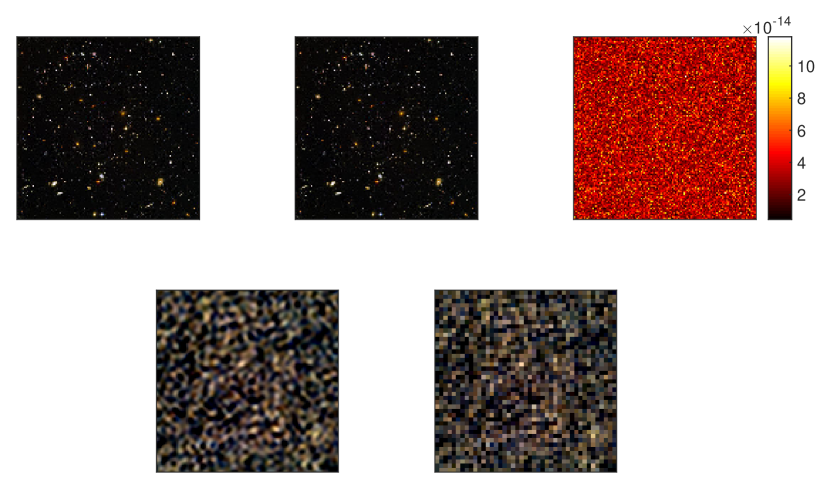
(a) Top row: The original $128\times 128$ HUDF image (left), reconstructed image (center), and the difference between normalized images (right),
Bottom row: blurred image (left), $3\mathsf{X}$ magnified subsampled blurred image (right)

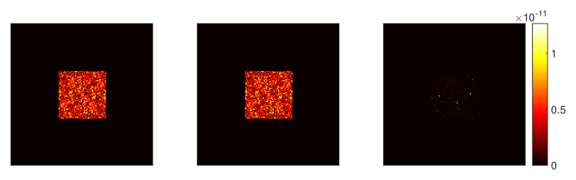
(b) Spectra of the original $128\times 128$ blur kernel (left), the reconstructed blur kernel (center), and the difference between normalized blur kernels (right)

Fig. 4: Blind deconvolution of a Hubble Ultra-Deep Field image and a synthetic blur kernel

In the second experiment we considered a more realistic model for the blur kernel. We use eight $64\times 64$ consecutive slices of a 3D Point Spread Function (PSF) in the Born & Wolf optical model that is generated by the PSFGenerator package [12] to create a subspace model for the target PSF. We used the default model parameters set by the package, except for the size of the PSF array in the XY plane mentioned above. Figure 5 depicts an orthonormal basis of the subspace (in magnitude) that we used in the experiment. We chose one of the original PSFs as our target PSF. Furthermore, we use a $128\times 128$ fluorescent microscopy image of endothelial cells as the target shown in Figure 7 (top left). For this experiment, the number of applied Rademacher masks is $K=200$. The subsampling is uniform in vertical and horizontal directions at the rate of $\frac{1}{8}$. Therefore, the number of observations per mask is $N=16\times 16$. To have a reference for comparison, the target image blurred by the target PSF and the $16\times 16$ subsampled version of the blurred image are shown in the bottom row of Figure 7.

Figure 6 illustrates the target PSF (left), the estimated PSF (center), and the error between the normalized target and the normalized estimated PSFs (right). Similarly, the top row of 7 illustrates the target image (left), the estimated image (center), and the error between the normalized target and the normalized estimated PSFs (right). As can be seen in these figures, the proposed blind deconvolution method has found accurate reconstructions of the PSF and the image. The relative error in the lifted domain is also in the order of $10^{-6}$.

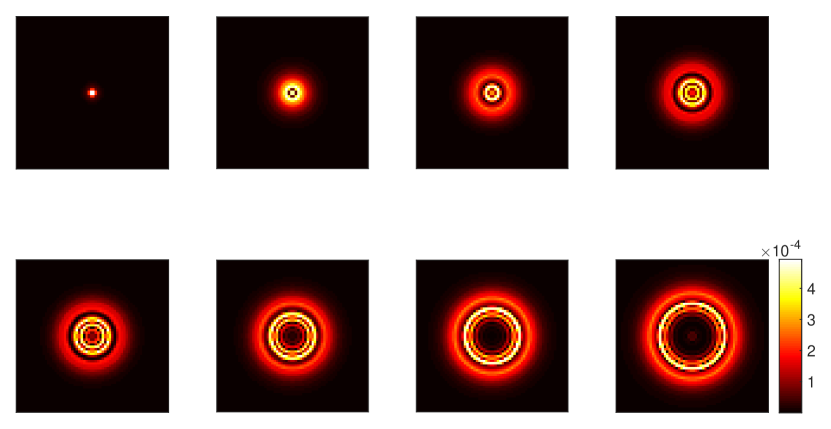
Fig. 5: The orthonormal basis for the PSF subspace shown in magnitude

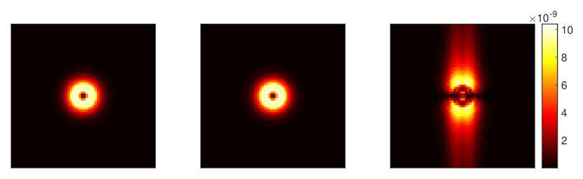
Fig. 6: The target PSF (left), the reconstructed PSF (center), and the difference between the normalized PSFs (right)

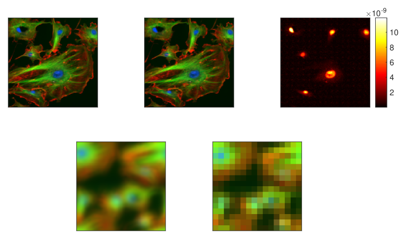
Fig. 7: Top row: image of fluorescent endothelial cells (left), reconstructed image (center), and the difference between the normalized images (right),
Bottom row: blurred image (left), $8\mathsf{X}$ magnified subsampled blurred image (right)

5 Conclusions

In this paper we studied the blind deconvolution problem in an imaging system that captures multiple instances of the target image modulated by randomly coded masks, blurred, and then spatially subsampled. We first expressed the necessary and sufficient condition for identifiability of the problem using a graph representation of the unknowns and the measurements. Furthermore, we formulate a different sufficient identifiability condition by considering a subspace model for the blurring kernel. Finally, under a special subspace model, namely the bandpass model, we derived the sufficient number of random masks that allow successful blind deconvolution through lifting and nuclear norm minimization.

An interesting extension to our work is to consider a subspace model for the image rather than the blurring kernel. We believe that this model would relax the identifiability requirements imposed on the blurring kernel that might not be appropriate in certain scenarios. The image subspace model can be further relaxed to sparsity with respect to some basis (e.g., wavelet, Fourier, etc). This subspace-sparse model would lead to estimation of simultaneously low-rank and row-sparse matrices in the lifted domain. These problems, in their general form, are known to be challenging and resistant to usual convex relaxation techniques [16]. However, we believe that the particular measurement model in the blind deconvolution problem can enable us to perform accurate and efficient blind deconvolution.

Appendix A Proofs of the results in Section 3.1

In this section we provide the proofs pertaining to the identifiability analysis provided in Section 3.1.

Proof of Lemma 1.  The assumptions made in Section 3.1 ensure that the isolated vertices in the considered bipartite graph correspond to the entries with value zero. Furthermore, for each edge of the graph we observe the product of its end nodes. Therefore, in each of the connected components of the graph, choosing the value of only one of the vertices is enough to uniquely determine the value of the other vertices of that component. This assignment of values does not depend on the other connected components of the graph. Therefore, if there are two or more connected components of order greater than one, each of them can take independent values. This implies that the corresponding matrix $\boldsymbol{h}\boldsymbol{x}^{\mathrm{T}}$ cannot be recovered uniquely.

Proof of Theorem 1.  As mentioned in Section 3.1, we have restricted our problem to scenarios where the measurements $x_{i}h_{j}$ for any particular $i$ and similarly for any particular $j$ cannot be simultaneously zero. Therefore, the zero entries of $\boldsymbol{x}$ (and also $\boldsymbol{h}$) can be easily identified from the zero measurements. By the assumption that $\boldsymbol{x}\neq 0$, there is at least one $1\leq i\leq L$ where $x_{i}\neq 0$ . Let $\left.\boldsymbol{h}\right|_{\mathsf{J}_{i}}$ denote the restriction of $\boldsymbol{h}$ to the entries indexed by $\mathsf{J}_{i}$. Therefore, we observe the vector $x_{i}\left.\boldsymbol{h}\right|_{\mathsf{J}_{i}}$ which is nonzero. Invoking the assumption that the restriction of $\boldsymbol{V}$ to the rows indexed by $\mathsf{J}_{i}$ is full-rank we deduce that we can recover the vector $x_{i}\boldsymbol{h}$, uniquely by solving a least squares problem. Then, it is straightforward to recover any remaining nonzero $x_{l}\boldsymbol{h}$ from the measurements.

Appendix B Proofs of the results in Section 3.2

B.1 Tools from probability theory

In this section we provide the definitions and results from probability theory that we frequently apply in the proofs.

Definition 1.

For a convex and non-decreasing function $\psi:\mathbb{R}_{+}\to\mathbb{R}_{+}$ that satisfies$\psi\left(0\right)=0$, the Orlicz $\psi$-norm for a random matrix (or vector) $\boldsymbol{X}$ is defined as

$$\left\|\boldsymbol{X}\right\|_{\psi} =\inf\left\{u>0\mid\mathbb{E}\left[\psi\left(\frac{\left\|\boldsymbol{X}\right\|}{u}\right)\right]\leq 1\right\}.$$

Some important special cases of the Orlicz $\psi$-norms are

• the Orlicz $2$-norm, also known as the sub-Gaussian norm, denoted by $\left\|\cdot\right\|_{\psi_{2}}$ with $\psi_{2}\left(t\right)=e^{\frac{t^{2}}{2}}-1$, and

• the Orlicz $1$-norm, also known as subexponential norm, denoted by $\left\|\cdot\right\|_{\psi_{1}}$ with $\psi_{1}\left(t\right)=e^{t}-1$.

Proposition 1 (Matrix Bernstein’s inequality [14, Proposition 2]).

Let $\boldsymbol{X}_{1},\boldsymbol{X}_{2},\dotsc,$ and $\boldsymbol{X}_{n}$ be independent random matrices of dimension $d_{1}\times d_{2}$ that satisfy $\mathbb{E}\left[\boldsymbol{X}_{i}\right]=\boldsymbol{0}$. Suppose that for $B>0$ we have

$$\max_{i=1,2,\dotsc,n}\left\|\boldsymbol{X}_{i}\right\|_{\psi_{1}} \leq B,$$

and define

$$\sigma^{2}: =\max\left\{\left\|\mathbb{E}\left[\sum_{i=1}^{n}\boldsymbol{X}_{i}\boldsymbol{X}_{i}^{*}\right]\right\|,\left\|\mathbb{E}\left[\sum_{i=1}^{n}\boldsymbol{X}_{i}^{*}\boldsymbol{X}_{i}\right]\right\|\right\}.$$

Then, there exist a constant $C$ such that for all $t\geq 0$ the tail bound

$$\left\|\sum_{i=1}^{n}\boldsymbol{X}_{i}\right\| \leq C\max\left\{\sigma\sqrt{t+\log\left(d_{1}+d_{2}\right)},B\log\left(\frac{\sqrt{n}B}{\sigma}\right)\left(t+\log\left(d_{1}+d_{2}\right)\right)\right\},$$

holds with probability at least $1-e^{-t}$.

Proposition 2 (Orlicz norm of a finite maximum [25, Lemma 2.2.2]).

Let $\psi$ be a convex, nondecreasing, nonzero function that obeys $\psi\left(0\right)=0$ and $\lim\sup_{x,y\to\infty}\psi\left(x\right)\psi\left(y\right)/\psi\left(cxy\right)<\infty$ for some constant $c$. Then, for any random variables $x_{1},x_{2},\dotsc,$ and $x_{n}$ we have

$$\left\|\max_{i=1,2,\dotsc,n}x_{i}\right\|_{\psi} \leq c_{\psi}\psi^{-1}\left(n\right)\max_{i=1,2,\dotsc,n}\left\|x_{i}\right\|_{\psi},$$

for some constant $c_{\psi}$ depending only on $\psi$.

Proposition 3 (Hanson-Wright inequality [21, Theorem 1.1]).

Let $\boldsymbol{x}\in\mathbb{R}^{n}$ be a random vector with independent components $x_{i}$ which satisfy $\mathbb{E}\left[x_{i}\right]=0$ and $\left\|x_{i}\right\|_{\psi_{2}}\leq\rho$. Let $\boldsymbol{A}$ be an $n\times n$ matrix. Then, for every $t\geq 0$,

$$\mathbb{P}\left\{\left|\boldsymbol{x}^{\mathrm{T}}\boldsymbol{A}\boldsymbol{x}-\mathbb{E}\left[\boldsymbol{x}^{\mathrm{T}}\boldsymbol{A}\boldsymbol{x}\right]\right|>t\right\} \leq 2e^{-c\min\left\{\frac{t^{2}}{\rho^{4}\left\|\boldsymbol{A}\right\|_{F}^{2}},\frac{t}{\rho^{2}\left\|\boldsymbol{A}\right\|}\right\}}.$$

B.2 Proof of Theorem 2

The auxiliary and intermediate lemmas needed for the proof of Theorem 2 are subsumed to the latter parts of this section. To prove the theorem we need to construct a dual certificate that exhibits certain properties on the “support set”

(8) $$\mathsf{T} =\left\{\widehat{\boldsymbol{h}}\boldsymbol{v}^{*}+\boldsymbol{u}\overline{\boldsymbol{x}}^{*}\mid\boldsymbol{u}\in\mathbb{C}^{N},\boldsymbol{v}\in\mathbb{C}^{L}\right\},$$

and its orthogonal complement $\mathsf{T}{}^{\perp}$.

Proof of Theorem 2.  Our proof begins by stating the conditions for unique recovery of $\widehat{\boldsymbol{h}}\overline{\boldsymbol{x}}^{*}$ from (7) which parallels the arguments in [1, Section 3.1]. Without repeating every detail explained in [1], we provide a sketch here for clarification. Recall that $\widehat{\boldsymbol{h}}$ and $\boldsymbol{x}$ are assumed to have unit $\ell_{2}$-norm. Let

$$\mathcal{P}_{\mathsf{T}}: \boldsymbol{S}\mapsto\widehat{\boldsymbol{h}}\widehat{\boldsymbol{h}}^{*}\boldsymbol{S}+\boldsymbol{S}\overline{\boldsymbol{x}}\overline{\boldsymbol{x}}^{*}-\widehat{\boldsymbol{h}}\widehat{\boldsymbol{h}}^{*}\boldsymbol{S}\overline{\boldsymbol{x}}\overline{\boldsymbol{x}}^{*},\qquad \mathcal{P}_{\mathsf{T}^{\perp}}: \boldsymbol{S}\mapsto\left(\boldsymbol{I}-\widehat{\boldsymbol{h}}\widehat{\boldsymbol{h}}^{*}\right)\boldsymbol{S}\left(\boldsymbol{I}-\overline{\boldsymbol{x}}\overline{\boldsymbol{x}}^{*}\right)$$

denote the orthognoal projections onto the subspaces $\mathsf{T}$ and $\mathsf{T}^{\perp}$, respectively. It can be shown that (see, e.g. [19]) the matrix $\widehat{\boldsymbol{h}}\overline{\boldsymbol{x}}^{*}$ is a unique minimizer of (7) if there exists a matrix $\boldsymbol{Y}\in\mathrm{range}\left(\mathcal{A}^{*}\right)$ such that

$$\Re\left\langle\widehat{\boldsymbol{h}}\overline{\boldsymbol{x}}^{*}-\mathcal{P}_{\mathsf{T}}\left(\boldsymbol{Y}\right),\mathcal{P}_{\mathsf{T}}\left(\boldsymbol{Z}\right)\right\rangle-\Re\left\langle\mathcal{P}_{\mathsf{T}^{\perp}}\left(\boldsymbol{Y}\right),\mathcal{P}_{\mathsf{T}^{\perp}}\left(\boldsymbol{Z}\right)\right\rangle+\left\|\mathcal{P}_{\mathsf{T}^{\perp}}\left(\boldsymbol{Z}\right)\right\|_{*} >0,$$

for all $\boldsymbol{Z}\in\mathrm{null}\left(\mathcal{A}\right)$. Applying Hölder’s inequality to the first two terms shows that it suffices to find a $\boldsymbol{Y}\in\mathrm{range}\left(\mathcal{A}^{*}\right)$ that satisfies

(9) $$-\left\|\widehat{\boldsymbol{h}}\overline{\boldsymbol{x}}^{*}-\mathcal{P}_{\mathsf{T}}\left(\boldsymbol{Y}\right)\right\|_{F}\left\|\mathcal{P}_{\mathsf{T}}\left(\boldsymbol{Z}\right)\right\|_{F}+\left(1-\left\|\mathcal{P}_{\mathsf{T}^{\perp}}\left(\boldsymbol{Y}\right)\right\|\right)\left\|\mathcal{P}_{\mathsf{T}^{\perp}}\left(\boldsymbol{Z}\right)\right\|_{*} >0,$$

for all $\boldsymbol{Z}\in\mathrm{null}\left(\mathcal{A}\right)$. Using the fact that $\boldsymbol{Z}\in\mathrm{null}\left(\mathcal{A}\right)$ and Lemma 2 below which guarantees

(10) $$\left|\left\|\mathcal{A}\left(\boldsymbol{X}\right)\right\|_{F}^{2}-\mathbb{E}\left[\left\|\mathcal{A}\left(\boldsymbol{X}\right)\right\|_{F}^{2}\right]\right| \leq\frac{1}{2}\left\|\boldsymbol{X}\right\|_{F}^{2}$$

for all $\boldsymbol{X}\in\mathsf{T}$, we can deduce that

$$0=\left\|\mathcal{A}\left(\boldsymbol{Z}\right)\right\|_{F} \geq\frac{1}{\sqrt{2}}\left\|\mathcal{P}_{\mathsf{T}}\left(\boldsymbol{Z}\right)\right\|_{F}-\left\|\mathcal{A}\right\|\left\|\mathcal{P}_{\mathsf{T}^{\perp}}\left(\boldsymbol{Z}\right)\right\|_{*}$$

holds with probability at least $1-3L^{-\beta}$ if $K\overset{\beta}{\gtrsim}\mu\log^{2}L\,\log\log\left(N+1\right)$ for some $\beta>0$. The bound (10) also guarantees that $\mathcal{P}_{\mathsf{T}^{\perp}}\left(\boldsymbol{Z}\right)=\boldsymbol{Z}-\mathcal{P}_{\mathsf{T}}\left(\boldsymbol{Z}\right)$ cannot be the zero matrix. Combining these results and (9) shows that it suffices to find a $\boldsymbol{Y}\in\mathrm{range}\left(\mathcal{A}^{*}\right)$ (i.e., the dual certificate) that obeys

(11) $$\sqrt{2}\left\|\mathcal{A}\right\|\left\|\mathcal{P}_{\mathsf{T}}\left(\boldsymbol{Y}\right)-\widehat{\boldsymbol{h}}\overline{\boldsymbol{x}}^{*}\right\|_{F} \leq\frac{1}{4}$$

and

(12) $$\left\|\mathcal{P}_{\mathsf{T}^{\perp}}\left(\boldsymbol{Y}\right)\right\| <\frac{3}{4}.$$

Similar to [1] we employ the golfing scheme [9] to construct the dual certificate $\boldsymbol{Y}$. Consider a partition of the the index set $\left\{1,2,\dotsc,K\right\}$ to its disjoint subsets $\mathsf{K}_{1},\mathsf{K}_{2},\dotsc$, and $\mathsf{K}_{P}$ such that

$$\left|\mathsf{K}_{p}\right| =\frac{K}{P}\quad\forall p\in\left\{1,2,\dotsc,P\right\}.$$

Define the operator restricted to indices in $\mathsf{K}_{p}$ as

(13) $$\mathcal{A}_{p}\left(\boldsymbol{X}\right) :=\sqrt{\frac{LP}{K}}\left(\boldsymbol{F}_{N}\odot\boldsymbol{X}\right)\boldsymbol{\Phi}_{\mathsf{K}_{p}}.$$

Furthermore, we obtain a sequence of matrices $\boldsymbol{Y}_{0}=\boldsymbol{0},\boldsymbol{Y}_{1},\dotsc,\boldsymbol{Y}_{P}$ through the recursive relation

$$\boldsymbol{Y}_{p} =\boldsymbol{Y}_{p-1}+\mathcal{A}_{p}^{*}\mathcal{A}_{p}\left(\widehat{\boldsymbol{h}}\overline{\boldsymbol{x}}^{*}-\mathcal{P}_{\mathsf{T}}\left(\boldsymbol{Y}_{p-1}\right)\right).$$

Our goal is to show that $\boldsymbol{Y}=\boldsymbol{Y}_{P}$ satisfies (11) and (12) with high probability. With

(14) $$\boldsymbol{W}_{p} :=\mathcal{P}_{\mathsf{T}}\left(\boldsymbol{Y}_{p}\right)-\widehat{\boldsymbol{h}}\overline{\boldsymbol{x}}^{*},$$

projecting both sides of the above recursion onto $\mathsf{T}$ yields

$$\boldsymbol{W}_{p} =\boldsymbol{W}_{p-1}-\mathcal{P}_{\mathsf{T}}\mathcal{A}_{p}^{*}\mathcal{A}_{p}\left(\boldsymbol{W}_{p-1}\right)$$

$$=\left(\mathcal{P}_{\mathsf{T}}-\mathcal{P}_{\mathsf{T}}\mathcal{A}_{p}^{*}\mathcal{A}_{p}\mathcal{P}_{\mathsf{T}}\right)\left(\boldsymbol{W}_{p-1}\right),$$

where the latter equation holds because $\boldsymbol{W}_{p-1}\in\mathsf{T}$ by construction. Therefore, with

$$\left|\mathsf{K}_{p}\right|=\frac{K}{P} \overset{\beta}{\gtrsim}\mu\log^{2}L\,\log\log\left(N+1\right),$$

we can invoke Lemma 2 below to guarantee that

$$\left\|\boldsymbol{W}_{p}\right\|_{F} \leq\frac{1}{2}\left\|\boldsymbol{W}_{p-1}\right\|_{F}\quad\forall p=1,2,\dotsc P,$$

and thus

(15) $$\left\|\boldsymbol{W}_{p}\right\|_{F} \leq 2^{-p}\left\|\widehat{\boldsymbol{h}}\overline{\boldsymbol{x}}^{*}\right\|_{F}=2^{-p}\quad\forall p=1,2,\dotsc,P,$$

hold with probability at least $1-3PL^{-\beta}$. This result implies that (11) holds for $\boldsymbol{Y}=\boldsymbol{Y}_{P}$ if

$$P \geq\log_{2}\left(4\sqrt{2}\left\|\mathcal{A}\right\|\right)=\frac{5}{2}+\log_{2}\left\|\mathcal{A}\right\|.$$

From Lemma 3 below we know that that $\left\|\mathcal{A}\right\|\lesssim 1+\sqrt{\frac{L}{K}}+\sqrt{\frac{\beta\log L}{K}}$ with probability at least $1-L^{-\beta}$. Therefore, we can deduce that with

(16) $$P \gtrsim\max\left\{1,\log\left(1+\sqrt{\frac{L}{K}}+\sqrt{\frac{\beta\log L}{K}}\right)\right\},$$

(11) holds for $\boldsymbol{Y}=\boldsymbol{Y}_{P}$ with probability exceeding $1-\left(3P+1\right)L^{-\beta}$.

To show that $\boldsymbol{Y}=\boldsymbol{Y}_{P}$ also obeys (12), we begin by expressing each $\boldsymbol{Y}_{P}$ explicitly in terms of the matrices $\boldsymbol{W}_{p}$ as

$$\boldsymbol{Y}_{P} =\sum_{p=1}^{P}\boldsymbol{Y}_{p}-\boldsymbol{Y}_{p-1}=-\sum_{p=1}^{P}\mathcal{A}_{p}^{*}\mathcal{A}_{p}\left(\boldsymbol{W}_{p-1}\right).$$

Then using the fact that $\mathcal{P}_{\mathsf{T}^{\perp}}\left(\boldsymbol{W}_{p-1}\right)=\boldsymbol{0}$ for all $p=1,2,\dotsc,P$ we can write

$$\left\|\mathcal{P}_{\mathsf{T}^{\perp}}\left(\boldsymbol{Y}_{P}\right)\right\| =\left\|\mathcal{P}_{\mathsf{T}^{\perp}}\left(\sum_{p=1}^{P}\mathcal{A}_{p}^{*}\mathcal{A}_{p}\left(\boldsymbol{W}_{p-1}\right)\right)\right\|$$

$$=\left\|\mathcal{P}_{\mathsf{T}^{\perp}}\left(\sum_{p=1}^{P}\mathcal{A}_{p}^{*}\mathcal{A}_{p}\left(\boldsymbol{W}_{p-1}\right)-\boldsymbol{W}_{p-1}\right)\right\|$$

$$\leq\left\|\sum_{p=1}^{P}\mathcal{A}_{p}^{*}\mathcal{A}_{p}\left(\boldsymbol{W}_{p-1}\right)-\boldsymbol{W}_{p-1}\right\|$$

$$\leq\sum_{p=1}^{P}\left\|\mathcal{A}_{p}^{*}\mathcal{A}_{p}\left(\boldsymbol{W}_{p-1}\right)-\boldsymbol{W}_{p-1}\right\|.$$

If the size of each partition $\mathsf{K}_{p}$ is sufficiently large and specifically obeys

(17) $$\frac{K}{P}=\left|\mathsf{K}_{p}\right| \overset{\beta}{\gtrsim}\mu\log^{2}L\log\log\left(N+1\right),$$

then we can apply Lemma 4, stated below in Section B.2.3, to simplify the bound on $\left\|\mathcal{P}_{\mathsf{T}^{\perp}}\left(\boldsymbol{Y}_{P}\right)\right\|$ and write

$$\left\|\mathcal{P}_{\mathsf{T}^{\perp}}\left(\boldsymbol{Y}_{P}\right)\right\| \leq\frac{3}{4}\sum_{p=1}^{P}2^{-p}<\frac{3}{4},$$

which holds with probability at least $1-cPL^{-\beta}$ where $c$ is an absolute constant. Therefore, if there exists a $P$ that satisfies both (16) and (17), then (11) and (12) simultaneously hold for $\boldsymbol{Y}=\boldsymbol{Y}_{P}$ with probability at least $1-c^{\prime}PL^{-\beta}$ for some absolute constant $c^{\prime}$. To guarantee existence of such $P$, it suffices to have

$$K \overset{\beta}{\gtrsim}\mu\log^{2}L\log\frac{Le}{\mu}\log\log\left(N+1\right),$$

for which we can choose $P\lesssim\log\frac{Le}{\mu}$. Since $\mu\geq L/N$ we have $P\lesssim N$. The probability of the desired events exceeds $1-O\left(NL^{-\beta}\right)$.

B.2.1 $\mathcal{A}_{p}$ is a near isometry on $\mathsf{T}$

We would like to show that the restriction of $\mathcal{A}_{p}$, defined by (13), to the subspace $\mathsf{T}$ in (8) has a near isometry behavior. In particular, our goal is to show that for all $\boldsymbol{X}\in\mathsf{T}$ the inequality

$$\left|\left\|\mathcal{A}_{p}\left(\boldsymbol{X}\right)\right\|_{F}^{2}-\mathbb{E}\left[\left\|\mathcal{A}_{p}\left(\boldsymbol{X}\right)\right\|_{F}^{2}\right]\right| \leq\frac{1}{2}\left\|\boldsymbol{X}\right\|_{F}^{2}$$

holds with high probability. The following lemma with $\mathsf{K}=\mathsf{K}_{p}$ establishes the desired property.

Lemma 2 (near isometry of $\mathcal{A}_{\mathsf{K}}$ on $\mathsf{T}$).

Let be $\mathsf{K}\subseteq\left\{1,2,\dotsc,K\right\}$ be an arbitrary index set and define

(18) $$\mathcal{A}_{\mathsf{K}}\left(\boldsymbol{X}\right) :=\sqrt{\frac{L}{\left|\mathsf{K}\right|}}\left(\boldsymbol{F}_{N}\odot\boldsymbol{X}\right)\boldsymbol{\Phi}_{\mathsf{K}}.$$

For any $\beta>0$, if we have

$$\left|\mathsf{K}\right| \overset{\beta}{\gtrsim}\mu\log^{2}L\,\log\log\left(N+1\right),$$

then

$$\left|\left\|\mathcal{A}_{\mathsf{K}}\left(\boldsymbol{X}\right)\right\|_{F}^{2}-\mathbb{E}\left[\left\|\mathcal{A}_{\mathsf{K}}\left(\boldsymbol{X}\right)\right\|_{F}^{2}\right]\right| \leq\frac{1}{2}\left\|\boldsymbol{X}\right\|_{F}^{2}$$

for all $\boldsymbol{X}\in\mathsf{T}$, with probability at least $1-3L^{-\beta}$.

Proof.

For every $\boldsymbol{X}=\widehat{\boldsymbol{h}}\boldsymbol{v}^{*}+\boldsymbol{u}\overline{\boldsymbol{x}}^{*}\in\mathsf{T}$ we have

$$\left\|\mathcal{A}_{\mathsf{K}}\left(\boldsymbol{X}\right)\right\|_{F}^{2}-\mathbb{E}\left[\left\|\mathcal{A}_{\mathsf{K}}\left(\boldsymbol{X}\right)\right\|_{F}^{2}\right] =\frac{L}{\left|\mathsf{K}\right|}\sum_{k\in\mathsf{K}}\mathrm{tr}\left(\left(\boldsymbol{F}{}_{N}\odot\boldsymbol{X}\right)\left(\boldsymbol{\phi}_{k}\boldsymbol{\phi}_{k}^{*}-\boldsymbol{I}\right)\left(\boldsymbol{F}{}_{N}\odot\boldsymbol{X}\right)^{*}\right)$$

$$=\frac{L}{\left|\mathsf{K}\right|}\sum_{k\in\mathsf{K}}\mathrm{tr}\left.\Bigl{(}\left(\boldsymbol{D}_{\widehat{\boldsymbol{h}}}\boldsymbol{F}_{N}\boldsymbol{D}_{\boldsymbol{v}}^{*}+\boldsymbol{D}_{\boldsymbol{u}}\boldsymbol{F}_{N}\boldsymbol{D}_{\boldsymbol{x}}\right)\left(\boldsymbol{\phi}_{k}\boldsymbol{\phi}_{k}^{*}-\boldsymbol{I}\right)\right.$$

$$\hskip 50.00008pt\left.\left(\boldsymbol{D}_{\boldsymbol{v}}\boldsymbol{F}_{N}^{*}\boldsymbol{D}_{\widehat{\boldsymbol{h}}}^{*}+\boldsymbol{D}_{\boldsymbol{x}}^{*}\boldsymbol{F}_{N}^{*}\boldsymbol{D}_{\boldsymbol{u}}^{*}\right)\right)$$

$$=\frac{L}{\left|\mathsf{K}\right|}\sum_{k\in\mathsf{K}}\mathrm{tr}\left(\boldsymbol{D}_{\widehat{\boldsymbol{h}}}\boldsymbol{F}_{N}\boldsymbol{D}_{\boldsymbol{v}}^{*}\left(\boldsymbol{\phi}_{k}\boldsymbol{\phi}_{k}^{*}-\boldsymbol{I}\right)\boldsymbol{D}_{\boldsymbol{v}}\boldsymbol{F}_{N}^{*}\boldsymbol{D}_{\widehat{\boldsymbol{h}}}^{*}\right)$$

$$+\frac{L}{\left|\mathsf{K}\right|}\sum_{k\in\mathsf{K}}\mathrm{tr}\left(\boldsymbol{D}_{\boldsymbol{u}}\boldsymbol{F}_{N}\boldsymbol{D}_{\boldsymbol{x}}\left(\boldsymbol{\phi}_{k}\boldsymbol{\phi}_{k}^{*}-\boldsymbol{I}\right)\boldsymbol{D}_{\boldsymbol{x}}^{*}\boldsymbol{F}_{N}^{*}\boldsymbol{D}_{\boldsymbol{u}}^{*}\right)$$

$$+\frac{L}{\left|\mathsf{K}\right|}\sum_{k\in\mathsf{K}}\mathrm{tr}\left(\boldsymbol{D}_{\widehat{\boldsymbol{h}}}\boldsymbol{F}_{N}\boldsymbol{D}_{\boldsymbol{v}}^{*}\left(\boldsymbol{\phi}_{k}\boldsymbol{\phi}_{k}^{*}-\boldsymbol{I}\right)\boldsymbol{D}_{\boldsymbol{x}}^{*}\boldsymbol{F}_{N}^{*}\boldsymbol{D}_{\boldsymbol{u}}^{*}\right)$$

(19) $$+\frac{L}{\left|\mathsf{K}\right|}\sum_{k\in\mathsf{K}}\mathrm{tr}\left(\boldsymbol{D}_{\boldsymbol{u}}\boldsymbol{F}_{N}\boldsymbol{D}_{\boldsymbol{x}}\left(\boldsymbol{\phi}_{k}\boldsymbol{\phi}_{k}^{*}-\boldsymbol{I}\right)\boldsymbol{D}_{\boldsymbol{v}}\boldsymbol{F}_{N}^{*}\boldsymbol{D}_{\widehat{\boldsymbol{h}}}^{*}\right).$$

Therefore, for all $\boldsymbol{X}\in\mathsf{T}$ we can write (19) as

$$\left\|\mathcal{A}_{\mathsf{K}}\left(\boldsymbol{X}\right)\right\|_{F}^{2}-\mathbb{E}\left[\left\|\mathcal{A}_{\mathsf{K}}\left(\boldsymbol{X}\right)\right\|_{F}^{2}\right] =\frac{1}{\left|\mathsf{K}\right|}\sum_{k\in\mathsf{K}}\left\langle\boldsymbol{Z}_{k},\overline{\boldsymbol{v}}\overline{\boldsymbol{v}}^{*}\right\rangle+\frac{1}{\left|\mathsf{K}\right|}\sum_{k\in\mathsf{K}}\left\langle\boldsymbol{Z}^{\prime}_{k},\overline{\boldsymbol{u}}\overline{\boldsymbol{u}}^{*}\right\rangle+\frac{2}{\left|\mathsf{K}\right|}\sum_{k\in\mathsf{K}}\Re\left\langle\boldsymbol{Z}^{\prime\prime}_{k},\overline{\boldsymbol{v}}\boldsymbol{u}^{*}\right\rangle.$$

where the summands are expressed using the matrices

(20) $$\boldsymbol{Z}_{k} =L\left(\boldsymbol{D}_{\boldsymbol{\phi}_{k}}^{*}\boldsymbol{F}_{N}^{*}\boldsymbol{D}_{\left|\widehat{\boldsymbol{h}}\right|^{2}}\boldsymbol{F}_{N}\boldsymbol{D}_{\boldsymbol{\phi}_{k}}-\frac{\left\|\widehat{\boldsymbol{h}}\right\|_{2}^{2}}{L}\boldsymbol{I}\right),$$

(21) $$\boldsymbol{Z}^{\prime}_{k} =L\mathrm{diag}\left(\boldsymbol{F}_{N}\boldsymbol{D}_{\boldsymbol{x}}\left(\boldsymbol{\phi}_{k}\boldsymbol{\phi}_{k}^{*}-\boldsymbol{I}\right)\boldsymbol{D}_{\boldsymbol{x}}^{*}\boldsymbol{F}_{N}^{*}\right),$$

and

(22) $$\boldsymbol{Z}^{\prime\prime}_{k} =L\left(\boldsymbol{D}_{\boldsymbol{\phi}_{k}}^{*}\boldsymbol{F}_{N}^{*}\boldsymbol{D}_{\widehat{\boldsymbol{h}}}^{*}\boldsymbol{D}_{\boldsymbol{F}_{N}\left(\boldsymbol{x}\odot\boldsymbol{\phi}_{k}\right)}-\frac{1}{L}\boldsymbol{x}\widehat{\boldsymbol{h}}^{*}\right)$$

Then, the triangle inequality yields

$$\left|\left\|\mathcal{A}_{\mathsf{K}}\left(\boldsymbol{X}\right)\right\|_{F}^{2}-\mathbb{E}\left[\left\|\mathcal{A}_{\mathsf{K}}\left(\boldsymbol{X}\right)\right\|_{F}^{2}\right]\right| \leq\frac{\left\|\boldsymbol{v}\right\|_{2}^{2}}{\left|\mathsf{K}\right|}\left\|\sum_{k\in\mathsf{K}}\boldsymbol{Z}{}_{k}\right\|+\frac{\left\|\boldsymbol{u}\right\|_{2}^{2}}{\left|\mathsf{K}\right|}\left\|\sum_{k\in\mathsf{K}}\boldsymbol{Z}^{\prime}_{k}\right\|+\frac{2\left\|\boldsymbol{u}\right\|_{2}\left\|\boldsymbol{v}\right\|_{2}}{\left|\mathsf{K}\right|}\left\|\sum_{k\in\mathsf{K}}\boldsymbol{Z}^{\prime\prime}_{k}\right\|.$$

Without loss of generality we can assume that $\boldsymbol{\overline{v}}$ is orthogonal to $\boldsymbol{x}$ which implies that

$$\left\|\boldsymbol{X}\right\|_{F}^{2} =\left\|\widehat{\boldsymbol{h}}\right\|_{2}^{2}\left\|\boldsymbol{v}\right\|_{2}^{2}+\left\|\boldsymbol{u}\right\|_{2}^{2}\left\|\boldsymbol{x}\right\|_{2}^{2}=\left\|\boldsymbol{u}\right\|_{2}^{2}+\left\|\boldsymbol{v}\right\|_{2}^{2},$$

and thereby

(23) $$\left|\left\|\mathcal{A}_{\mathsf{K}}\left(\boldsymbol{X}\right)\right\|_{F}^{2}-\mathbb{E}\left[\left\|\mathcal{A}_{\mathsf{K}}\left(\boldsymbol{X}\right)\right\|_{F}^{2}\right]\right| \leq\frac{1}{\left|\mathsf{K}\right|}\left(\left\|\sum_{k\in\mathsf{K}}\boldsymbol{Z}{}_{k}\right\|+\left\|\sum_{k\in\mathsf{K}}\boldsymbol{Z}^{\prime}_{k}\right\|+\left\|\sum_{k\in\mathsf{K}}\boldsymbol{Z}^{\prime\prime}_{k}\right\|\right)\left\|\boldsymbol{X}\right\|_{F}^{2},$$

holds for all $\boldsymbol{X}\in\mathsf{T}$. Therefore, it suffices to bound the operator norm of the sums of $\boldsymbol{Z}_{k}$s, $\boldsymbol{Z}^{\prime}_{k}$s, and $\boldsymbol{Z}^{\prime\prime}_{k}$s, separately. As shown by Lemmas 6, 7, and 8 in Section B.3, the matrix Bernstein’s inequality can be used to establish the desired bounds. It follows from these lemmas that for $\left|\mathsf{K}\right|\overset{\beta}{\gtrsim}\mu\log^{2}L\,\log\log\left(N+1\right)$, the bound

$$\left|\left\|\mathcal{A}_{\mathsf{K}}\left(\boldsymbol{X}\right)\right\|_{F}^{2}-\mathbb{E}\left[\left\|\mathcal{A}_{\mathsf{K}}\left(\boldsymbol{X}\right)\right\|_{F}^{2}\right]\right| \leq\frac{1}{2}\left\|\boldsymbol{X}\right\|_{F}^{2}$$

holds for all $\boldsymbol{X}\in\mathsf{T}$ with probability at least $1-3L^{-\beta}$. ∎

B.2.2 Operator norm of $\mathcal{A}$

The following lemma establishes a global bound for the operator norm of $\mathcal{A}$ that holds with high probability.

Lemma 3 (the operator norm of $\mathcal{A}$).

For any $\beta>0$, the operator norm of $\mathcal{A}$ can be bounded as

$$\left\|\mathcal{A}\right\| \lesssim\sqrt{\frac{L}{K}}+\sqrt{\frac{\beta\log L}{K}}$$

with probability at least $1-L^{-\beta}$.

Proof.

By definition we have

$$\left\|\mathcal{A}\right\| =\sup_{\boldsymbol{X}\neq\boldsymbol{0}}\frac{\left\|\mathcal{A}\left(\boldsymbol{X}\right)\right\|_{F}}{\left\|\boldsymbol{X}\right\|_{F}}$$

$$=\sup_{\boldsymbol{X}\neq\boldsymbol{0}}\frac{\left\|\sqrt{\frac{L}{K}}\left(\boldsymbol{F}_{N}\odot\boldsymbol{X}\right)\boldsymbol{\Phi}\right\|_{F}}{\left\|\boldsymbol{X}\right\|_{F}}$$

$$\leq\sqrt{\frac{L}{K}}\left\|\boldsymbol{\Phi}\right\|\sup_{\boldsymbol{X}\neq\boldsymbol{0}}\frac{\left\|\left(\boldsymbol{F}_{N}\odot\boldsymbol{X}\right)\right\|_{F}}{\left\|\boldsymbol{X}\right\|_{F}}$$

$$=\frac{1}{\sqrt{K}}\left\|\boldsymbol{\Phi}\right\|,$$

where the last inequality holds because $\left\|\boldsymbol{F}_{N}\odot\boldsymbol{X}\right\|_{F}=\frac{1}{\sqrt{L}}\left\|\boldsymbol{X}\right\|_{F}$. Therefore, we can use standard tail bounds for the spectral norm of random matrices with independent sub-Gaussian entries to bound $\left\|\boldsymbol{\Phi}\right\|$ and thus $\left\|\mathcal{A}\right\|$. For example, the bound established in [20, Proposition 2.4] guarantees that for any $t>0$ we have

$$\left\|\boldsymbol{\Phi}\right\| \leq C\left(\sqrt{L}+\sqrt{K}\right)+t$$

with probability at least $1-2e^{-ct^{2}}$, where $C$ and $c$ are absolute constants. Therefore, setting $t=\sqrt{\frac{\beta\log L+\log 2}{c}}$ we can show that

$$\left\|\boldsymbol{\Phi}\right\| \lesssim\sqrt{L}+\sqrt{K}+\sqrt{\beta\log L}$$

holds with probability at least $1-L^{-\beta}$. This completes the proof. ∎

B.2.3 Decay of $\left\|\mathcal{A}_{p}^{*}\mathcal{A}_{p}\left(\boldsymbol{W}_{p-1}\right)-\boldsymbol{W}_{p-1}\right\|$ with respect to $p$

Our goal in this section is to show that for $\mathcal{A}_{p}$s defined by (13) and $\boldsymbol{W}_{p}$s defined by (14), with high probability, the quantity $\left\|\mathcal{A}_{p}^{*}\mathcal{A}_{p}\left(\boldsymbol{W}_{p-1}\right)-\boldsymbol{W}_{p-1}\right\|$ decays quickly as $p$ increases.

Lemma 4.

For $p=0,1,\dotsc,P-1$ let $\boldsymbol{W}_{p}$ be defined by (14). Then we can choose

$$\left|\mathsf{K}_{p}\right| \overset{\beta}{\gtrsim}\mu\log^{2}L\log\log\left(N+1\right),$$

such that

$$\left\|\mathcal{A}_{p}^{*}\mathcal{A}_{p}\left(\boldsymbol{W}_{p-1}\right)-\boldsymbol{W}_{p-1}\right\| \leq\frac{3}{4}\cdot 2^{-p}$$

holds for every $p$ simultaneously with probability at least $1-cPL^{-\beta}$ where $c>0$ is an absolute constant.

Proof.

The action of $\mathcal{A}_{p}^{*}\mathcal{A}_{p}$ on the matrix $\boldsymbol{W}_{p-1}$ obeys

$$\mathcal{A}_{p}^{*}\mathcal{A}_{p}\left(\boldsymbol{W}_{p-1}\right)-\boldsymbol{W}_{p-1} =L\overline{\boldsymbol{F}}_{N}\odot\left(\left(\boldsymbol{F}_{N}\odot\boldsymbol{W}_{p-1}\right)\left(\frac{1}{\left|\mathsf{K}_{p}\right|}\boldsymbol{\Phi}_{\mathsf{K}_{p}}\boldsymbol{\Phi}_{\mathsf{K}_{p}}^{*}-\boldsymbol{I}\right)\right)$$

$$=\frac{1}{\left|\mathsf{K}_{p}\right|}\sum_{k\in\mathsf{K}_{p}}L\overline{\boldsymbol{F}}_{N}\odot\left(\left(\boldsymbol{F}_{N}\odot\boldsymbol{W}_{p-1}\right)\left(\boldsymbol{\phi}_{k}\boldsymbol{\phi}_{k}^{*}-\boldsymbol{I}\right)\right).$$

Since $\boldsymbol{W}_{p-1}\in\mathsf{T}$ we can find vectors $\boldsymbol{u}$ and $\boldsymbol{v}$ such that

$$\boldsymbol{W}_{p-1} =\widehat{\boldsymbol{h}}\boldsymbol{v}^{*}+\boldsymbol{u}\overline{\boldsymbol{x}}^{*},$$

which implies that

$$\mathcal{A}_{p}^{*}\mathcal{A}_{p}\left(\boldsymbol{W}_{p-1}\right)-\boldsymbol{W}_{p-1} =\frac{1}{\left|\mathsf{K}_{p}\right|}\sum_{k\in\mathsf{K}_{p}}L\overline{\boldsymbol{F}}_{N}\odot\left(\left(\boldsymbol{F}_{N}\odot\left(\widehat{\boldsymbol{h}}\boldsymbol{v}^{*}+\boldsymbol{u}\overline{\boldsymbol{x}}^{*}\right)\right)\left(\boldsymbol{\phi}_{k}\boldsymbol{\phi}_{k}^{*}-\boldsymbol{I}\right)\right).$$

Without loss of generality, we also assume that $\boldsymbol{x}$ and $\boldsymbol{\overline{v}}$ are orthogonal so that

$$\left\|\boldsymbol{W}_{p-1}\right\|_{F}^{2} =\left\|\widehat{\boldsymbol{h}}\boldsymbol{v}^{*}\right\|_{F}^{2}+\left\|\boldsymbol{u}\overline{\boldsymbol{x}}^{*}\right\|_{F}^{2}=\left\|\boldsymbol{v}\right\|_{2}^{2}+\left\|\boldsymbol{u}\right\|_{2}^{2}.$$

Therefore, on the event that the near isometry of $\mathcal{A}_{p}$ on $\mathsf{T}$ as stated by the Lemma 2 holds, the bound in (15) guarantees that

(24) $$\left\|\boldsymbol{u}\right\|_{2}^{2}+\left\|\boldsymbol{v}\right\|_{2}^{2} \leq 2^{-2p}.$$

Furthermore, we can write

(25) $$\mathcal{A}_{p}^{*}\mathcal{A}_{p}\left(\boldsymbol{W}_{p-1}\right)-\boldsymbol{W}_{p-1} =\frac{1}{\left|\mathsf{K}_{p}\right|}\left(\sum_{k\in\mathsf{K}_{p}}\widetilde{\boldsymbol{Z}}_{k}+\sum_{k\in\mathsf{K}_{p}}\widetilde{\boldsymbol{Z}}^{\prime}_{k}\right)$$

where

$$\widetilde{\boldsymbol{Z}}_{k} :=L\overline{\boldsymbol{F}}_{N}\odot\left(\left(\boldsymbol{F}_{N}\odot\left(\widehat{\boldsymbol{h}}\boldsymbol{v}^{*}\right)\right)\left(\boldsymbol{\phi}_{k}\boldsymbol{\phi}_{k}^{*}-\boldsymbol{I}\right)\right)$$

$$=L\boldsymbol{D}_{\widehat{\boldsymbol{h}}}\boldsymbol{D}_{\boldsymbol{F}_{N}\left(\overline{\boldsymbol{v}}\odot\boldsymbol{\phi}_{k}\right)}\overline{\boldsymbol{F}}_{N}\boldsymbol{D}_{\phi_{k}}^{*}-\widehat{\boldsymbol{h}}\boldsymbol{v}^{*}$$

and

$$\widetilde{\boldsymbol{Z}}^{\prime}_{k} :=L\overline{\boldsymbol{F}}_{N}\odot\left(\left(\boldsymbol{F}_{N}\odot\left(\boldsymbol{u}\overline{\boldsymbol{x}}^{*}\right)\right)\left(\boldsymbol{\phi}_{k}\boldsymbol{\phi}_{k}^{*}-\boldsymbol{I}\right)\right)$$

$$=L\boldsymbol{D}_{\boldsymbol{u}}\boldsymbol{D}_{\boldsymbol{F}_{N}\left(\boldsymbol{x}\odot\boldsymbol{\phi}_{k}\right)}\overline{\boldsymbol{F}}_{N}\boldsymbol{D}_{\boldsymbol{\phi}_{k}}^{*}-\boldsymbol{u}\overline{\boldsymbol{x}}^{*}.$$

These matrices are very similar to the matrix $\boldsymbol{Z}^{\prime\prime}_{k}$ defined by (22). In fact, if we consider $\boldsymbol{Z}^{\prime\prime}_{k}$ to be a function of $\boldsymbol{x}$ and $\boldsymbol{\widehat{\boldsymbol{h}}}$ such as $\boldsymbol{Z}^{\prime\prime}_{k}\left(\boldsymbol{x},\widehat{\boldsymbol{h}}\right)$, then it is easy to verify that

$$\widetilde{\boldsymbol{Z}_{k}} =\left(\boldsymbol{Z}^{\prime\prime}_{k}\left(\overline{\boldsymbol{v}},\overline{\boldsymbol{\widehat{h}}}\right)\right)^{\mathrm{T}},$$

and

$$\widetilde{\boldsymbol{Z}}^{\prime}_{k} =\left(\boldsymbol{Z}^{\prime\prime}_{k}\left(\boldsymbol{x},\overline{\boldsymbol{u}}\right)\right)^{\mathrm{T}}.$$

Therefore, we can readily use Lemma 8 in Section B.3 to obtain bounds for the spectral norms of the sum of $\widetilde{\boldsymbol{Z}}_{k}$s and the sum of $\widetilde{\boldsymbol{Z}}^{\prime}_{k}$s. To adapt the result of Lemma 8, it suffices to scale the deviation bounds by the norm of the vectors $\boldsymbol{u}$ or $\boldsymbol{v}$ and replace the coherence of $\widehat{\boldsymbol{h}}$ by that of $\boldsymbol{u}$, as necessary.

As explained above, we can use Lemma 8 and (25) to obtain

$$\left\|\mathcal{A}_{p}^{*}\mathcal{A}_{p}\left(\boldsymbol{W}_{p-1}\right)-\boldsymbol{W}_{p-1}\right\| \leq\frac{1}{\left|\mathsf{K}_{p}\right|}\left(\left\|\sum_{k\in\mathsf{K}_{p}}\widetilde{\boldsymbol{Z}}_{k}\right\|+\left\|\sum_{k\in\mathsf{K}_{p}}\widetilde{\boldsymbol{Z}}^{\prime}_{k}\right\|\right)$$

$$\overset{\beta}{\lesssim}\left\|\boldsymbol{v}\right\|_{2}\max\left\{\sqrt{\frac{\mu}{\left|\mathsf{K}_{p}\right|}\log L},\frac{\sqrt{\mu}\log L\log\left(N+1\right)\,\log\log\left(N+1\right)}{\left|\mathsf{K}_{p}\right|}\right\}$$

$$+\max\left\{\sqrt{\frac{L\left\|\boldsymbol{u}\right\|_{\infty}^{2}}{\left|\mathsf{K}_{p}\right|}\log L},\right.$$

$$\hskip 50.00008pt\left.\frac{\sqrt{L\left\|\boldsymbol{u}\right\|_{\infty}^{2}}\log L\log\left(N+1\right)\,\log\log\left(N+1\right)}{\left|\mathsf{K}_{p}\right|}\right\},$$

with probability at least $1-2L^{-\beta}$. We define $\mu_{p-1}$, a quantity that controls the largest row-wise energy of $\boldsymbol{W}_{p-1}$, by

(26) $$\mu_{p-1} :=L\left\|\boldsymbol{W}_{p-1}\right\|_{\infty,2}^{2},$$

where $\left\|\cdot\right\|_{\infty,2}$ denotes the largest row-wise $\ell_{2}$-norm. Since $\boldsymbol{u}=\boldsymbol{W}_{p-1}\overline{\boldsymbol{x}}$ and $\overline{\boldsymbol{x}}$ is unit-norm, it is straightforward to show that

$$\left\|\boldsymbol{u}\right\|_{\infty}^{2} \leq\frac{\mu_{p-1}}{L},$$

and rewrite the bound on $\left\|\mathcal{A}_{p}^{*}\mathcal{A}_{p}\left(\boldsymbol{W}_{p-1}\right)-\boldsymbol{W}_{p-1}\right\|$ as

$$\left\|\mathcal{A}_{p}^{*}\mathcal{A}_{p}\left(\boldsymbol{W}_{p-1}\right)-\boldsymbol{W}_{p-1}\right\| \overset{\beta}{\lesssim}\left\|\boldsymbol{v}\right\|_{2}\max\left\{\sqrt{\frac{\mu}{\left|\mathsf{K}_{p}\right|}\log L},\frac{\sqrt{\mu}\log L\log\left(N+1\right)\,\log\log\left(N+1\right)}{\left|\mathsf{K}_{p}\right|}\right\}$$

$$+\max\left\{\sqrt{\frac{\mu_{p-1}}{\left|\mathsf{K}_{p}\right|}\log L},\right.$$

$$\hskip 50.00008pt\left.\frac{\sqrt{\mu_{p-1}}\log L\log\left(N+1\right)\,\log\log\left(N+1\right)}{\left|\mathsf{K}_{p}\right|}\Biggl{\}}\right..$$

The inequality (24) implies that $\left\|\boldsymbol{u}\right\|_{2}\leq 2^{-p}$ and $\left\|\boldsymbol{v}\right\|_{2}\leq 2^{-p}$. Furthermore, if we have

$$\left|\mathsf{K}_{p}\right| \overset{\beta}{\gtrsim}\mu\log^{2}L\log\log\left(N+1\right),$$

then we can invoke Lemma 5 below to guarantee the bound $\mu_{p-1}\leq 2^{-2p}\mu$ with probability exceeding $1-2L^{-\beta}$. Therefore, the above deviation bound can be simplified to

$$\left\|\mathcal{A}_{p}^{*}\mathcal{A}_{p}\left(\boldsymbol{W}_{p-1}\right)-\boldsymbol{W}_{p-1}\right\| \overset{\beta}{\lesssim}2^{-p}\max\left\{\sqrt{\frac{\mu}{\left|\mathsf{K}_{p}\right|}\log L},\frac{\sqrt{\mu}\log L\log\left(N+1\right)\,\log\log\left(N+1\right)}{\left|\mathsf{K}_{p}\right|}\right\}$$

$$\leq\frac{3}{4}\cdot 2^{-p}.$$

The events that the above inequality depends on for every $p=1,2,\dotsc,P$, hold simultaneously with probability exceeding $1-cPL^{-\beta}$ where $c>0$ is an absolute constant. ∎

B.2.4 Controlling the largest row-norm of $\boldsymbol{W}_{p}$

Through the following lemma we show that the largest row-wise $\ell_{2}$-norm of $\boldsymbol{W}_{p}$ decreases significantly as $p$ increases.

Lemma 5.

For $p=1,2,\dotsc,P$, let $\mu_{p}$ be defined as (26). Furthermore, suppose that

$$\mu_{p-1} \leq 2^{-2\left(p-1\right)}\mu.$$

Then, with $\left|\mathsf{K}_{p}\right|\overset{\beta}{\gtrsim}\mu\log^{2}L\,\log\log\left(N+1\right)$ we have

$$\mu_{p} \leq 2^{-2p}\mu,$$

with probability at least $1-2L^{-\beta}$. Therefore, we have

$$\mu_{p} \leq 2^{-2p}\mu,$$

simultaneously for all $p=1,2,\dotsc,P$ with probability at least $1-2PL^{-\beta}$.

Proof.

Let $\boldsymbol{R}_{p}:=\boldsymbol{W}_{p-1}-\mathcal{A}_{p}^{*}\mathcal{A}_{p}\left(\boldsymbol{W}_{p-1}\right)$. Furthermore, denote the $l$-th columns of $\boldsymbol{R}_{p}^{*}$, $\boldsymbol{W}_{p-1}^{*}$, and $\boldsymbol{W}_{p}^{*}$ by $\boldsymbol{r}_{l,p}$, $\boldsymbol{w}_{l,p-1}$, and $\boldsymbol{w}_{l,p}$, respectively. Because $\boldsymbol{W}_{p}=\mathcal{P}_{\mathsf{T}}\left(\boldsymbol{R}_{p}\right)$, it follows from Lemma 10 in Section B.3 that

$$\left\|\boldsymbol{w}_{l,p}\right\|_{2}^{2} \leq\left\|\widehat{\boldsymbol{h}}\right\|_{\infty}^{2}\left\|\boldsymbol{R}_{p}^{*}\widehat{\boldsymbol{h}}\right\|_{2}^{2}+\left|\left\langle\overline{\boldsymbol{x}},\boldsymbol{r}_{l,p}\right\rangle\right|^{2}$$

(27) $$=\frac{\mu}{L}\left\|\boldsymbol{R}_{p}^{*}\widehat{\boldsymbol{h}}\right\|_{2}^{2}+\left|\left\langle\overline{\boldsymbol{x}},\boldsymbol{r}_{l,p}\right\rangle\right|^{2}.$$

We can expand $\boldsymbol{R}_{p}$ as

$$\boldsymbol{R}_{p} =\frac{1}{\left|\mathsf{K}_{p}\right|}\sum_{k\in\mathsf{K}_{p}}\boldsymbol{W}_{p-1}-L\overline{\boldsymbol{F}}_{N}\odot\left(\left(\boldsymbol{F}_{N}\odot\boldsymbol{W}_{p-1}\right)\boldsymbol{\phi}_{k}\boldsymbol{\phi}_{k}^{*}\right)$$

$$=\frac{1}{\left|\mathsf{K}_{p}\right|}\sum_{k\in\mathsf{K}_{p}}\boldsymbol{W}_{p-1}-L\overline{\boldsymbol{F}}_{N}\odot\left(\left(\boldsymbol{F}_{N}\odot\boldsymbol{W}_{p-1}\right)\boldsymbol{\phi}_{k}\boldsymbol{\phi}_{k}^{*}\right).$$

Therefore, we can write

$$\boldsymbol{R}_{p}^{*}\widehat{\boldsymbol{h}} =\frac{1}{\left|\mathsf{K}_{p}\right|}\sum_{k\in\mathsf{K}_{p}}\left(\boldsymbol{W}_{p-1}^{*}-L\overline{\boldsymbol{F}}_{N}^{*}\odot\left(\boldsymbol{\phi}_{k}\boldsymbol{\phi}_{k}^{*}\left(\boldsymbol{F}_{N}^{*}\odot\boldsymbol{W}_{p-1}^{*}\right)\right)\right)\widehat{\boldsymbol{h}}$$

$$=\frac{1}{\left|\mathsf{K}_{p}\right|}\sum_{k\in\mathsf{K}_{p}}\boldsymbol{W}_{p-1}^{*}\widehat{\boldsymbol{h}}-L\boldsymbol{D}_{\boldsymbol{\phi}_{k}}\overline{\boldsymbol{F}}_{N}^{*}\left(\overline{\left(\boldsymbol{F}_{N}\odot\boldsymbol{W}_{p-1}\right)\boldsymbol{\phi}_{k}}\odot\widehat{\boldsymbol{h}}\right)$$

$$=\frac{1}{\left|\mathsf{K}_{p}\right|}\sum_{k\in\mathsf{K}_{p}}\boldsymbol{W}_{p-1}^{*}\widehat{\boldsymbol{h}}-L\boldsymbol{D}_{\boldsymbol{\phi}_{k}}\overline{\boldsymbol{F}}_{N}^{*}\left(\overline{\left(\boldsymbol{F}_{N}\odot\boldsymbol{W}_{p-1}\right)\boldsymbol{\phi}_{k}}\odot\widehat{\boldsymbol{h}}\right)$$

$$=\frac{1}{\left|\mathsf{K}_{p}\right|}\sum_{k\in\mathsf{K}_{p}}\boldsymbol{z}_{k},$$

where

(28) $$\boldsymbol{z}_{k} :=\boldsymbol{W}_{p-1}^{*}\widehat{\boldsymbol{h}}-L\boldsymbol{D}_{\boldsymbol{\phi}_{k}}\overline{\boldsymbol{F}}_{N}^{*}\left(\overline{\left(\boldsymbol{F}_{N}\odot\boldsymbol{W}_{p-1}\right)\boldsymbol{\phi}_{k}}\odot\widehat{\boldsymbol{h}}\right)$$

Conditioned on $\mathcal{A}_{1},\mathcal{A}_{2},\dotsc,$ and $\mathcal{A}_{p-1}$, we can invoke Lemma 9 below and show that

(29) $$\left\|\boldsymbol{R}_{p}^{*}\widehat{\boldsymbol{h}}\right\|_{2}^{2} \overset{\beta}{\lesssim}2^{-2\left(p-1\right)}\max\left\{\frac{\mu\log L}{\left|\mathsf{K}_{p}\right|},\frac{\mu\log^{2}\left(N+1\right)\log^{2}\log\left(N+1\right)\log^{2}L}{\left|\mathsf{K}_{p}\right|^{2}}\right\}$$

holds with probability exceeding $1-L^{-\beta}$. Furthermore, we can expand $\left\langle\overline{\boldsymbol{x}},\boldsymbol{r}_{l,p}\right\rangle$ as

$$\left\langle\overline{\boldsymbol{x}},\boldsymbol{r}_{l,p}\right\rangle =\frac{1}{\left|\mathsf{K}_{p}\right|}\sum_{k\in\mathsf{K}_{p}}\left\langle\overline{\boldsymbol{x}},\boldsymbol{w}_{l,p-1}\right\rangle-L\left\langle\overline{\boldsymbol{x}},\overline{\boldsymbol{f}_{l}}\odot\boldsymbol{\phi}_{k}\right\rangle\left\langle\overline{\boldsymbol{f}_{l}}\odot\boldsymbol{\phi}_{k},\boldsymbol{w}_{l,p-1}\right\rangle$$

$$=\frac{1}{\left|\mathsf{K}_{p}\right|}\sum_{k\in\mathsf{K}_{p}}\left\langle\overline{\boldsymbol{x}},\boldsymbol{w}_{l,p-1}\right\rangle-L\left\langle\boldsymbol{f}_{l}\odot\overline{\boldsymbol{x}},\boldsymbol{\phi}_{k}\right\rangle\left\langle\boldsymbol{\phi}_{k},\boldsymbol{f}_{l}\odot\boldsymbol{w}_{l,p-1}\right\rangle$$

$$=-\frac{1}{\left|\mathsf{K}_{p}\right|}\sum_{k\in\mathsf{K}_{p}}\zeta_{k},$$

with

$$\zeta_{k} :=L\left\langle\boldsymbol{f}_{l}\odot\overline{\boldsymbol{x}},\boldsymbol{\phi}_{k}\right\rangle\left\langle\boldsymbol{\phi}_{k},\boldsymbol{f}_{l}\odot\boldsymbol{w}_{l,p-1}\right\rangle-\left\langle\overline{\boldsymbol{x}},\boldsymbol{w}_{l,p-1}\right\rangle.$$

The Orlicz 1-norm of $\zeta_{k}$ can be bounded using Lemma 12 below as

$$\left\|\zeta_{k}\right\|_{\psi_{1}} \lesssim\left\|\boldsymbol{w}_{l,p-1}\right\|_{2}\left\|\boldsymbol{x}\right\|_{2}=\left\|\boldsymbol{w}_{l,p-1}\right\|_{2}.$$

Furthermore, we have

$$\mathbb{E}\left[\sum_{k\in\mathsf{K}_{p}}\left|\zeta_{k}\right|^{2}\right] =\left|\mathsf{K}_{p}\right|\left(L^{2}\mathbb{E}\left[\left|\left\langle\boldsymbol{f}_{l}\odot\overline{\boldsymbol{x}},\boldsymbol{\phi}_{k}\right\rangle\right|^{2}\left|\left\langle\boldsymbol{\phi}_{k},\boldsymbol{f}_{l}\odot\boldsymbol{w}_{l,p-1}\right\rangle\right|^{2}\right]-\left|\left\langle\overline{\boldsymbol{x}},\boldsymbol{w}_{l,p-1}\right\rangle\right|^{2}\right)$$

$$\leq 3\left|\mathsf{K}_{p}\right|\left\|\boldsymbol{w}_{l,p-1}\right\|_{2}^{2},$$

where Lemma 11 in Section B.3 is used to obtain the inequality. Therefore, the scalar Bernstein’s inequality guarantees that

$$\left|\sum_{k\in\mathsf{K}_{p}}\zeta_{k}\right| \lesssim\max\left\{\left\|\boldsymbol{w}_{l,p-1}\right\|_{2}\sqrt{3\left|\mathsf{K}_{p}\right|\left(t+\log 2\right)},\left\|\boldsymbol{w}_{l,p-1}\right\|_{2}\log\left(t+\log 2\right)\right\}$$

with probability at least $1-e^{-t}$. With $t=\beta\log L+\log N$, we deduce that

$$\left|\left\langle\overline{\boldsymbol{x}},\boldsymbol{r}_{l,p}\right\rangle\right|^{2} =\left(\frac{1}{\left|\mathsf{K}_{p}\right|}\left|\sum_{k\in\mathsf{K}_{p}}\zeta_{k}\right|\right)^{2}$$

(30) $$\overset{\beta}{\lesssim}\left\|\boldsymbol{w}_{l,p-1}\right\|_{2}^{2}\max\left\{\frac{\log L}{\left|\mathsf{K}_{p}\right|},\frac{\log^{2}L}{\left|\mathsf{K}_{p}\right|^{2}}\right\},$$

holds with probability exceeding $1-N^{-1}L^{-\beta}$.

The inequalities (27), (29), and (30), and the assumption

$$L\left\|\boldsymbol{w}_{l,p-1}\right\|_{2}^{2} \leq\mu_{p-1}\leq\mu 2^{-2\left(p-1\right)}$$

show that

$$L\left\|\boldsymbol{w}_{l,p}\right\|_{2}^{2}\overset{\beta}{\lesssim} 2^{-2\left(p-1\right)}\mu\max\left\{\frac{\mu\log L}{\left|\mathsf{K}_{p}\right|},\frac{\mu\log^{2}\left(N+1\right)\log^{2}\log\left(N+1\right)\log^{2}L}{\left|\mathsf{K}_{p}\right|^{2}}\right\}$$

$$+2^{-2\left(p-1\right)}\mu\max\left\{\frac{\log L}{\left|\mathsf{K}_{p}\right|},\frac{\log^{2}L}{\left|\mathsf{K}_{p}\right|^{2}}\right\}$$

holds with probability at least $1-2N^{-1}L^{-\beta}$. Then using the assumption that $\left|\mathsf{K}_{p}\right|\overset{\beta}{\gtrsim}\mu\log^{2}L\,\log\log\left(N+1\right)$ and applying the union bound over $l$ guarantees that

$$\mu_{p}\leq 2^{-2p}\mu,$$

with probability exceeding $1-2L^{-\beta}$. Finally, since $\mu_{0}=L\left\|\boldsymbol{W}_{0}\right\|_{\infty,2}^{2}=L\left\|\widehat{\boldsymbol{h}}\right\|^{2}=\mu$, a recursive application of the above bound guarantees that

$$\mu_{p} \leq 2^{-2p}\mu,$$

for $p=1,2,\dotsc P$ hold simultaneously with probability exceeding $1-2PL^{-\beta}$. ∎

B.3 Supplementary lemmas

The proofs in this section rely on a form of the matrix Bernstein’s inequality borrowed from [14] and stated in Proposition 1.

Lemma 6.

For any $\beta>0$ the matrices $\boldsymbol{Z}_{k}$, defined by (20), obey

$$\left\|\sum_{k\in\mathsf{K}}\boldsymbol{Z}_{k}\right\| \overset{\beta}{\lesssim}\max\left\{\sqrt{\left|\mathsf{K}\right|\mu\log L},\mu\log\mu\log L\right\},$$

with probability at least $1-L^{-\beta}$.

Proof.

Since $\left\|\boldsymbol{Z}_{k}\right\|\leq L\left\|\widehat{\boldsymbol{h}}\right\|_{\infty}^{2}=\mu$, then

$$\max_{k\in\mathsf{K}}\left\|\boldsymbol{Z}_{k}\right\|_{\psi_{1}} \leq B:=\frac{\mu}{\log 2}.$$

Furthermore, we have

$$\mathbb{E}\left[\boldsymbol{Z}_{k}^{2}\right] =L^{2}\left(\frac{\left\|\widehat{\boldsymbol{h}}\right\|_{4}^{4}}{L}\boldsymbol{I}-\frac{\left\|\widehat{\boldsymbol{h}}\right\|_{2}^{4}}{L^{2}}\boldsymbol{I}\right)$$

from which we obtain the bound

$$\left\|\mathbb{E}\left[\sum_{k\in\mathsf{K}}\boldsymbol{Z}_{k}^{2}\right]\right\| \leq\sigma^{2}:=\left|\mathsf{K}\right|\mu.$$

Therefore, for any $t>0$ the matrix Bernstein’s inequality guarantees that

$$\left\|\sum_{k\in\mathsf{K}}\boldsymbol{Z}_{k}\right\| \leq C\max\left\{\sigma\sqrt{t+\log 2L},B\log\left(\frac{\sqrt{\left|\mathsf{K}\right|}B}{\sigma}\right)\left(t+\log 2L\right)\right\}$$

$$=C\max\left\{\sqrt{\left|\mathsf{K}\right|\mu\left(t+\log 2L\right)},\frac{\mu}{\log 2}\log\left(\frac{\sqrt{\mu}}{\log 2}\right)\left(t+\log 2L\right)\right\}$$

with probability at least $1-e^{-t}$. In particular, with $t=\beta\log L$ we obtain

$$\left\|\sum_{k\in\mathsf{K}}\boldsymbol{Z}_{k}\right\| \overset{\beta}{\lesssim}\max\left\{\sqrt{\left|\mathsf{K}\right|\mu\log L},\mu\log\mu\log L\right\}$$

with probability at least $1-L^{-\beta}$.∎

Lemma 7.

For any $\beta>0$ the matrices $\boldsymbol{Z}^{\prime}_{k}$, as defined by (21), obey

$$\left\|\sum_{k\in\mathsf{K}}\boldsymbol{Z}^{\prime}_{k}\right\| \overset{\beta}{\lesssim}\max\left\{\sqrt{\left|\mathsf{K}\right|\log L},\log^{2}L\right\},$$

with probability at least $1-L^{-\beta}$.

Proof.

Note that $\boldsymbol{Z}^{\prime}_{k}=L\left(\boldsymbol{D}_{\left|\boldsymbol{F}_{N}\left(\boldsymbol{x}\odot\boldsymbol{\phi}_{k}\right)\right|^{2}}-\frac{\left\|\boldsymbol{x}\right\|_{2}^{2}}{L}\boldsymbol{I}\right)$ using which we deduce that

$$\left\|\boldsymbol{Z}^{\prime}_{k}\right\| \leq L\max_{l=1,2,\dotsc,N}\left|\left|\left\langle\boldsymbol{\phi}_{k},\overline{\boldsymbol{x}}\odot\boldsymbol{f}_{l}\right\rangle\right|^{2}-\frac{\left\|\boldsymbol{x}\right\|_{2}^{2}}{L}\right|.$$

Therefore, the Orlicz 1-norm of the right-hand side is an upper bound for that of $\boldsymbol{Z}^{\prime}_{k}$. Using Proposition 2, we can thus show that

$$\left\|\boldsymbol{Z}^{\prime}_{k}\right\|_{\psi_{1}} \leq c_{\psi_{1}}L\log\left(N+1\right)\max_{l=1,2,\dotsc,N}\left\|\left|\left|\left\langle\boldsymbol{\phi}_{k},\overline{\boldsymbol{x}}\odot\boldsymbol{f}_{l}\right\rangle\right|^{2}-\frac{\left\|\boldsymbol{x}\right\|_{2}^{2}}{L}\right|\right\|_{\psi_{1}},$$

for some absolute constant $c_{\psi_{1}}>0$ depending only on the function $\psi_{1}\left(u\right)=e^{u}-1$. Applying Lemma 12 below to the latter inequality then yields

$$\left\|\boldsymbol{Z}^{\prime}_{k}\right\|_{\psi_{1}} \leq 8c_{\psi_{1}}\log\left(N+1\right)$$

and thereby

$$\max_{k\in\mathsf{K}}\left\|\boldsymbol{Z}^{\prime}_{k}\right\|_{\psi_{1}} \leq B:=8c_{\psi_{1}}\log\left(N+1\right).$$

Furthermore, we have

$$\mathbb{E}\left[\boldsymbol{Z}_{k}^{\prime 2}\right] =L^{2}\left(\mathbb{E}\left[\boldsymbol{D}_{\left|\boldsymbol{F}_{N}\left(\boldsymbol{x}\odot\boldsymbol{\phi}_{k}\right)\right|^{4}}\right]-\frac{\left\|\boldsymbol{x}\right\|_{2}^{4}}{L^{2}}\boldsymbol{I}\right)$$

$$=L^{2}\left(\boldsymbol{D}_{\mathbb{E}\left[\left|\boldsymbol{F}_{N}\left(\boldsymbol{x}\odot\boldsymbol{\phi}_{k}\right)\right|^{4}\right]}-\frac{\left\|\boldsymbol{x}\right\|_{2}^{4}}{L^{2}}\boldsymbol{I}\right)$$

$$\preccurlyeq 2L^{2}\left(\frac{\left\|\boldsymbol{x}\right\|_{2}^{4}}{L^{2}}-\frac{\left\|\boldsymbol{x}\right\|_{4}^{4}}{L^{2}}\boldsymbol{I}\right)$$

$$\preccurlyeq 2\boldsymbol{I}$$

where the first matrix inequality follows from Lemma 11 below. The above inequality then yields

$$\left\|\mathbb{E}\left[\sum_{k\in\mathsf{K}}\boldsymbol{Z}_{k}^{\prime 2}\right]\right\| \leq\sigma^{2}:=2\left|\mathsf{K}\right|.$$

Applying the matrix Bernstein’s inequality for $t>0$ shows that that

$$\left\|\sum_{k\in\mathsf{K}}\boldsymbol{Z}_{k}^{\prime}\right\| \leq C^{\prime}\max\left\{\sigma\sqrt{t+\log 2N},B\log\left(\frac{\sqrt{\left|\mathsf{K}\right|}B}{\sigma}\right)\left(t+\log 2N\right)\right\}$$

$$=C^{\prime}\max\left\{\sqrt{2\left|\mathsf{K}\right|\left(t+\log 2N\right)},8c_{\psi_{1}}\log\left(N+1\right)\log\left(\frac{8c_{\psi_{1}}\log\left(N+1\right)}{\sqrt{2}}\right)\left(t+\log 2N\right)\right\}$$

with probability at least $1-e^{-t}$. Setting $t=\beta\log L$ we obtain

$$\left\|\sum_{k\in\mathsf{K}}\boldsymbol{Z}^{\prime}_{k}\right\| \overset{\beta}{\lesssim}\max\left\{\sqrt{\left|\mathsf{K}\right|\log L},\log L\log\left(N+1\right)\log\log\left(N+1\right)\right\}$$

with probability at least $1-L^{-\beta}$.∎

Lemma 8.

For any $\beta>0$ the matrices $\boldsymbol{Z}^{\prime\prime}_{k}$, as defined by (22), obey

$$\left\|\sum_{k\in\mathsf{K}}\boldsymbol{Z}^{\prime\prime}_{k}\right\| \overset{\beta}{\lesssim}\max\left\{\sqrt{\mu\left|\mathsf{K}\right|\log L},\sqrt{\mu}\log L\log\left(N+1\right)\,\log\log\left(N+1\right)\right\},$$

with probability at least $1-L^{-\beta}$.

Proof.

Using the triangle inequality we have

$$\left\|\boldsymbol{Z}^{\prime\prime}_{k}\right\|_{\psi_{1}} \leq L\left\|\boldsymbol{D}_{\boldsymbol{\phi}_{k}}^{*}\boldsymbol{F}_{N}^{*}\boldsymbol{D}_{\widehat{\boldsymbol{h}}}^{*}\boldsymbol{D}_{\boldsymbol{F}_{N}\left(\boldsymbol{x}\odot\boldsymbol{\phi}_{k}\right)}\right\|_{\psi_{1}}+\left\|\boldsymbol{x}\widehat{\boldsymbol{h}}^{*}\right\|_{\psi_{1}}.$$

Straightforward bounds for the spectral norm yield

$$\left\|\boldsymbol{D}_{\boldsymbol{\phi}_{k}}^{*}\boldsymbol{F}_{N}^{*}\boldsymbol{D}_{\widehat{\boldsymbol{h}}}^{*}\boldsymbol{D}_{\boldsymbol{F}_{N}\left(\boldsymbol{x}\odot\boldsymbol{\phi}_{k}\right)}\right\| \leq\left\|\widehat{\boldsymbol{h}}\right\|_{\infty}\left\|\boldsymbol{F}_{N}\left(\boldsymbol{x}\odot\boldsymbol{\phi}_{k}\right)\right\|_{\infty},$$

using which we can write

$$\left\|\boldsymbol{Z}^{\prime\prime}_{k}\right\|_{\psi_{1}} \leq L\left\|\widehat{\boldsymbol{h}}\right\|_{\infty}\left\|\max_{l=1,2,\dotsc,N}\left|\left\langle\boldsymbol{\phi}_{k},\overline{\boldsymbol{x}}\odot\boldsymbol{f}_{l}\right\rangle\right|\right\|_{\psi_{1}}+\frac{1}{\log 2}$$

$$=\sqrt{L\mu}\left\|\max_{l=1,2,\dotsc,N}\left|\left\langle\boldsymbol{\phi}_{k},\overline{\boldsymbol{x}}\odot\boldsymbol{f}_{l}\right\rangle\right|\right\|_{\psi_{1}}+\frac{1}{\log 2}.$$

The Orlicz 1-norm on the right-hand side can be bounded using Proposition 2. Therefore, we have

$$\left\|\max_{l=1,2,\dotsc,N}\left|\left\langle\boldsymbol{\phi}_{k},\overline{\boldsymbol{x}}\odot\boldsymbol{f}_{l}\right\rangle\right|\right\|_{\psi_{1}} \leq c_{\psi_{1}}\log\left(N+1\right)\max_{l=1,2,\dotsc,N}\left\|\left|\left\langle\boldsymbol{\phi}_{k},\overline{\boldsymbol{x}}\odot\boldsymbol{f}_{l}\right\rangle\right|\right\|_{\psi_{1}}$$

for some absolute constant $c_{\psi_{1}}>0$ that only depends on the function $\psi_{1}\left(u\right)=e^{u}-1$. Lemma 13 below guarantees that

$$\left\|\left|\left\langle\boldsymbol{\phi}_{k},\overline{\boldsymbol{x}}\odot\boldsymbol{f}_{l}\right\rangle\right|\right\|_{\psi_{1}} \leq\frac{8}{\sqrt{L}}.$$

Thus, for each $k$ we have

$$\left\|\boldsymbol{Z}^{\prime\prime}_{k}\right\|_{\psi_{1}} \leq\left(8c_{\psi_{1}}+1\right)\frac{\sqrt{\mu}\log\left(N+1\right)}{\log 2},$$

or equivalently

$$\max_{k\in\mathcal{\mathsf{K}}}\left\|\boldsymbol{Z}^{\prime\prime}_{k}\right\|_{\psi_{1}} \leq B:=\left(8c_{\psi_{1}}+1\right)\frac{\sqrt{\mu}\log\left(N+1\right)}{\log 2}.$$

Furthermore, we have

$$\mathbb{E}\left[\boldsymbol{Z}_{k}^{\prime\prime*}\boldsymbol{Z}_{k}^{\prime\prime}\right] =L^{2}\mathbb{E}\left[\boldsymbol{D}_{\left|\widehat{\boldsymbol{h}}\odot\boldsymbol{F}_{N}\left(\boldsymbol{x}\odot\boldsymbol{\phi}_{k}\right)\right|^{2}}\right]-\widehat{\boldsymbol{h}}\widehat{\boldsymbol{h}}^{*}$$

$$=L\left\|\boldsymbol{x}\right\|_{2}^{2}\boldsymbol{D}_{\left|\widehat{\boldsymbol{h}}\right|^{2}}-\widehat{\boldsymbol{h}}\widehat{\boldsymbol{h}}^{*}$$

which implies that

$$\left\|\mathbb{E}\left[\sum_{k\in\mathsf{K}}\boldsymbol{Z}_{k}^{\prime\prime*}\boldsymbol{Z}_{k}^{\prime\prime}\right]\right\| \leq\left|\mathsf{K}\right|L\left\|\widehat{\boldsymbol{h}}\right\|_{\infty}^{2}=\left|\mathsf{K}\right|\mu.$$

We also have

$$\mathbb{E}\left[\boldsymbol{Z}_{k}^{\prime\prime}\boldsymbol{Z}_{k}^{\prime\prime*}\right] =L^{2}\mathbb{E}\left[\boldsymbol{D}_{\boldsymbol{\phi}_{k}}^{*}\boldsymbol{F}_{N}^{*}\boldsymbol{D}_{\left|\widehat{\boldsymbol{h}}\odot\boldsymbol{F}_{N}\left(\boldsymbol{x}\odot\boldsymbol{\phi}_{k}\right)\right|^{2}}\boldsymbol{F}_{N}\boldsymbol{D}_{\boldsymbol{\phi}_{k}}\right]-\boldsymbol{x}\boldsymbol{x}^{*}$$

which results in

$$\left\|\mathbb{E}\left[\sum_{k\in\mathsf{K}}\boldsymbol{Z}_{k}^{\prime\prime}\boldsymbol{Z}_{k}^{\prime\prime*}\right]\right\| \leq\left|\mathsf{K}\right|L^{2}\max_{\boldsymbol{u}:\left\|\boldsymbol{u}\right\|_{2}=1}\mathbb{E}\left[\sum_{l=1}^{N}\left|\widehat{h}_{l}\right|^{2}\left|\left\langle\boldsymbol{\phi}_{k},\boldsymbol{f}_{l}\odot\overline{\boldsymbol{x}}\right\rangle\right|^{2}\left|\left\langle\boldsymbol{\phi}_{k},\boldsymbol{f}_{l}\odot\overline{\boldsymbol{u}}\right\rangle\right|^{2}\right]$$

$$\leq\left|\mathsf{K}\right|L^{2}\max_{\boldsymbol{u}:\left\|\boldsymbol{u}\right\|_{2}=1}\sum_{l=1}^{N}\left|\widehat{h}_{l}\right|^{2}\!\left(3\left\|\boldsymbol{f}_{l}\odot\boldsymbol{x}\right\|_{2}^{2}\left\|\boldsymbol{f}_{l}\odot\overline{\boldsymbol{u}}\right\|_{2}^{2}-2\left\langle\left|\boldsymbol{f}_{l}\odot\overline{\boldsymbol{x}}\right|^{2}\!,\left|\boldsymbol{f}_{l}\odot\overline{\boldsymbol{u}}\right|^{2}\right\rangle\right)$$

$$\leq\left|\mathsf{K}\right|L^{2}\max_{\boldsymbol{u}:\left\|\boldsymbol{u}\right\|_{2}=1}\sum_{l=1}^{N}3\left|\widehat{h}_{l}\right|^{2}\left\|\boldsymbol{f}_{l}\odot\overline{\boldsymbol{x}}\right\|_{2}^{2}\left\|\boldsymbol{f}_{l}\odot\overline{\boldsymbol{u}}\right\|_{2}^{2}$$

$$=3\left|\mathsf{K}\right|$$

where we used Lemma 11 below in the second inequality. Therefore, we obtain

$$\max\left\{\left\|\mathbb{E}\left[\sum_{k\in\mathsf{K}}\boldsymbol{Z}_{k}^{\prime\prime*}\boldsymbol{Z}_{k}^{\prime\prime}\right]\right\|,\left\|\mathbb{E}\left[\sum_{k\in\mathsf{K}}\boldsymbol{Z}_{k}^{\prime\prime}\boldsymbol{Z}_{k}^{\prime\prime*}\right]\right\|\right\} \leq\sigma^{2}:=\max\left\{\mu,3\right\}\left|\mathsf{K}\right|.$$

Applying the matrix Bernstein’s inequality for $t>0$ shows that

$$\left\|\sum_{k\in\mathsf{K}}\boldsymbol{Z}_{k}^{\prime\prime}\right\| \leq C^{\prime\prime}\max\left\{\sigma\sqrt{t+\log\left(N+L\right)},B\log\left(\frac{\sqrt{\left|\mathsf{K}\right|}B}{\sigma}\right)\left(t+\log\left(N+L\right)\right)\right\}$$

$$=C^{\prime\prime}\max\left\{\sqrt{\left|\mathsf{K}\right|\left(t+\log\left(N+L\right)\right)\max\left\{\mu,3\right\}},\right.$$

$$\left.\left(8c_{\psi_{1}}+1\right)\frac{\sqrt{\mu}\log\left(N+1\right)}{\log 2}\log\left(\frac{\left(8c_{\psi_{1}}+1\right)\log\left(N+1\right)}{\log 2}\right)\left(t+\log\left(N+L\right)\right)\right\}$$

with probability at least $1-e^{-t}$. Setting $t=\beta\log L$ we obtain

$$\left\|\sum_{k\in\mathsf{K}}\boldsymbol{Z}^{\prime\prime}_{k}\right\| \overset{\beta}{\lesssim}\max\left\{\sqrt{\left|\mathsf{K}\right|\mu\log L},\sqrt{\mu}\log L\log\left(N+1\right)\,\log\log\left(N+1\right)\right\},$$

with probability at least $1-L^{-\beta}$. ∎

Lemma 9.

Let $\boldsymbol{z}_{k}$ and $\mu_{p-1}$ be defined as in (28) and (26), respectively. Furthermore, as in Lemma 5, suppose that $\mu_{p-1}\leq 2^{-2p+2}\mu$. Then, conditioned on $\mathcal{A}_{1},\mathcal{A}_{2},\dotsc,$ and $\mathcal{A}_{p-1}$, for $\beta>0$ we have

$$\left\|\sum_{k\in\mathsf{K}_{p}}\boldsymbol{z}_{k}\right\|_{2}\overset{\beta}{\lesssim} 2^{-p+1}\max\left\{\sqrt{\left|\mathsf{K}_{p}\right|\mu\log L},\sqrt{\mu}\log\left(N+1\right)\log\log\left(N+1\right)\,\log L\right\}$$

with probability at least $1-N^{-1}L^{-\beta}$.

Proof.

Applying the triangle inequality to (28) yields

(31) $$\left\|\boldsymbol{z}_{k}\right\|_{\psi_{1}} \leq B:=\left\|\boldsymbol{W}_{p-1}^{*}\widehat{\boldsymbol{h}}\right\|_{\psi_{1}}+L\left\|\boldsymbol{D}_{\boldsymbol{\phi}_{k}}\overline{\boldsymbol{F}}_{N}^{*}\left(\overline{\left(\boldsymbol{F}_{N}\odot\boldsymbol{W}_{p-1}\right)\boldsymbol{\phi}_{k}}\odot\widehat{\boldsymbol{h}}\right)\right\|_{\psi_{1}}.$$

The first term on the right-hand side of (31) can be bounded as

$$\left\|\boldsymbol{W}_{p-1}^{*}\widehat{\boldsymbol{h}}\right\|_{\psi_{1}} \leq\frac{\left\|\boldsymbol{W}_{p-1}^{*}\widehat{\boldsymbol{h}}\right\|_{2}}{\log 2}\leq\frac{\left\|\boldsymbol{W}_{p-1}^{*}\right\|\left\|\widehat{\boldsymbol{h}}\right\|_{2}}{\log 2}\leq\frac{2^{-p+1}}{\log 2},$$

where the last inequality follows from the bound $\left\|\boldsymbol{W}_{p-1}\right\|_{F}\leq 2^{-p+1}$ that is established using Lemma 2. Let $\boldsymbol{w}_{l,p-1}$ denote the $l$-th column of $\boldsymbol{W}_{p-1}^{*}$. The second term on the right hand side of (31) can also be bounded as

$$L\left\|\boldsymbol{D}_{\boldsymbol{\phi}_{k}}\overline{\boldsymbol{F}}_{N}^{*}\left(\overline{\left(\boldsymbol{F}_{N}\odot\boldsymbol{W}_{p-1}\right)\boldsymbol{\phi}_{k}}\odot\widehat{\boldsymbol{h}}\right)\right\|_{\psi_{1}} =L\left\|\overline{\left(\boldsymbol{F}_{N}\odot\boldsymbol{W}_{p-1}\right)\boldsymbol{\phi}_{k}}\odot\widehat{\boldsymbol{h}}\right\|_{\psi_{1}}=L\left\|\boldsymbol{D}_{\left(\boldsymbol{F}_{N}\odot\boldsymbol{W}_{p-1}\right)\boldsymbol{\phi}_{k}}^{*}\widehat{\boldsymbol{h}}\right\|_{\psi_{1}}$$

$$\leq L\left\|\max_{l=1,2,\dotsc,N}\left|\left\langle\boldsymbol{f}_{l}\odot\boldsymbol{w}_{l,p-1},\boldsymbol{\phi}_{k}\right\rangle\right|\left\|\widehat{\boldsymbol{h}}\right\|_{2}\right\|_{\psi_{1}}$$

$$\lesssim L\log\left(N+1\right)\max_{l=1,2,\dotsc,N}\left\|\left|\left\langle\boldsymbol{f}_{l}\odot\boldsymbol{w}_{l,p-1},\boldsymbol{\phi}_{k}\right\rangle\right|\right\|_{\psi_{1}}$$

$$\lesssim L\log\left(N+1\right)\max_{l=1,2,\dotsc,N}\left\|\boldsymbol{f}_{l}\odot\boldsymbol{w}_{l,p-1}\right\|_{2}$$

$$=\sqrt{L}\log\left(N+1\right)\max_{l=1,2,\dotsc,N}\left\|\boldsymbol{w}_{l,p-1}\right\|_{2}=\sqrt{\mu_{p-1}}\log\left(N+1\right)$$

$$\leq\sqrt{\mu}\log\left(N+1\right)2^{-p+1},$$

where the first through sixth lines respectively hold because of the fact that $\left\|\boldsymbol{D}_{\phi_{k}}\overline{\boldsymbol{F}}_{N}^{*}\boldsymbol{a}\right\|_{2}=\left\|\boldsymbol{a}\right\|_{2}$ for any $\boldsymbol{a}\in\mathbb{C}^{N}$, an elementary property of the spectral norm, Proposition 2, Lemma 13, the definition of $\mu_{p-1}$, and the assumed bound on $\mu_{p-1}$. Therefore, we deduce that $B$ in (31) obeys

$$B \lesssim\sqrt{\mu}\log\left(N+1\right)2^{-p+1}.$$

To apply the matrix Bernstein’s inequality we also need to upperbound the spectral norm of the expectation of the sum of the terms $\boldsymbol{z}_{k}^{*}\boldsymbol{z}_{k}$, and the sum of the terms $\boldsymbol{z}_{k}\boldsymbol{z}_{k}^{*}$. To bound the first spectral norm we can write

$$\left\|\mathbb{E}\left[\sum_{k\in\mathsf{K}_{p}}\boldsymbol{z}_{k}^{*}\boldsymbol{z}_{k}\right]\right\| =\left|\mathsf{K}_{p}\right|\mathbb{E}\left[\left\|\boldsymbol{z}_{k}\right\|_{2}^{2}\right]$$

$$=\left|\mathsf{K}_{p}\right|L^{2}\mathbb{E}\left[\left\|\overline{\left(\boldsymbol{F}_{N}\odot\boldsymbol{W}_{p-1}\right)\boldsymbol{\phi}_{k}}\odot\widehat{\boldsymbol{h}}\right\|_{2}^{2}\right]-\left|\mathsf{K}_{p}\right|\left\|\boldsymbol{W}_{p-1}^{*}\widehat{\boldsymbol{h}}\right\|_{2}^{2}$$

$$=\sum_{l=1}^{N}\left|\mathsf{K}_{p}\right|L\left\|\boldsymbol{w}_{l,p-1}\right\|_{2}^{2}\left|\widehat{h}_{l}\right|^{2}-\left|\mathsf{K}_{p}\right|\left\|\boldsymbol{W}_{p-1}^{*}\widehat{\boldsymbol{h}}\right\|_{2}^{2}$$

$$\leq\left|\mathsf{K}_{p}\right|L\left\|\widehat{\boldsymbol{h}}\right\|_{\infty}^{2}\sum_{l=1}^{N}\left\|\boldsymbol{w}_{l,p-1}\right\|_{2}^{2}$$

$$=\left|\mathsf{K}_{p}\right|\mu\left\|\boldsymbol{W}_{p-1}\right\|_{F}^{2}$$

$$\leq 2^{-2p+2}\left|\mathsf{K}_{p}\right|\mu.$$

Furthermore, the second spectral norm can be bounded as

$$\left\|\mathbb{E}\left[\sum_{k\in\mathsf{K}_{p}}\boldsymbol{z}_{k}\boldsymbol{z}_{k}^{*}\right]\right\| =\left|\mathsf{K}_{p}\right|\left\|\mathbb{E}\left[\boldsymbol{z}_{k}\boldsymbol{z}_{k}^{*}\right]\right\|$$

$$=\left|\mathsf{K}_{p}\right|\max_{\boldsymbol{u}:\left\|\boldsymbol{u}\right\|_{2}=1}L^{2}\mathbb{E}\left[\left|\left\langle\boldsymbol{u},\boldsymbol{z}_{k}\right\rangle\right|^{2}\right]$$

$$=\left|\mathsf{K}_{p}\right|\max_{\boldsymbol{u}:\left\|\boldsymbol{u}\right\|_{2}=1}L^{2}\mathbb{E}\left[\left|\sum_{l=1}^{N}\widehat{h}_{l}\left\langle\boldsymbol{\phi}_{k},\boldsymbol{f}_{l}\odot\boldsymbol{u}\right\rangle\left\langle\boldsymbol{f}_{l}\odot\boldsymbol{w}_{l,p-1},\boldsymbol{\phi}_{k}\right\rangle\right|^{2}\right]-\left|\widehat{\boldsymbol{h}}^{*}\boldsymbol{W}_{p-1}\boldsymbol{u}\right|^{2}$$

$$\leq\left|\mathsf{K}_{p}\right|\max_{\boldsymbol{u}:\left\|\boldsymbol{u}\right\|_{2}=1}L^{2}\mathbb{E}\left[N\sum_{l=1}^{N}\left|\widehat{h}_{l}\right|^{2}\left|\left\langle\boldsymbol{\phi}_{k},\boldsymbol{f}_{l}\odot\boldsymbol{u}\right\rangle\right|^{2}\left|\left\langle\boldsymbol{f}_{l}\odot\boldsymbol{w}_{l,p-1},\boldsymbol{\phi}_{k}\right\rangle\right|^{2}\right]$$

$$\leq\left|\mathsf{K}_{p}\right|\max_{\boldsymbol{u}:\left\|\boldsymbol{u}\right\|_{2}=1}L^{2}\mathbb{E}\left[N\left\|\widehat{\boldsymbol{h}}\right\|_{\infty}^{2}\sum_{l=1}^{N}\left|\left\langle\boldsymbol{\phi}_{k},\boldsymbol{f}_{l}\odot\boldsymbol{u}\right\rangle\right|^{2}\left|\left\langle\boldsymbol{f}_{l}\odot\boldsymbol{w}_{l,p-1},\boldsymbol{\phi}_{k}\right\rangle\right|^{2}\right]$$

$$\leq\left|\mathsf{K}_{p}\right|LN\mu\sum_{l=1}^{N}\frac{3\left\|\boldsymbol{w}_{l,p-1}\right\|_{2}^{2}}{L^{2}}$$

$$=3\left|\mathsf{K}_{p}\right|\frac{N}{L}\mu\left\|\boldsymbol{W}_{p-1}\right\|_{F}^{2}$$

$$\leq 3\cdot 2^{-2p+2}\left|\mathsf{K}_{p}\right|\frac{N}{L}\mu,$$

where the first inequality follows from the Cauchy-Schwarz inequality and the fact that $\left|\widehat{\boldsymbol{h}}^{*}\boldsymbol{W}_{p-1}\boldsymbol{u}\right|^{2}\geq 0$, the second inequality follows from the Hölder’s inequality applied to the sum inside the expectation, and the third inequality follows from Lemma 11 below. Therefore, we have

$$\sigma^{2}:=\max\left\{\left\|\mathbb{E}\left[\sum_{k\in\mathsf{K}_{p}}\boldsymbol{z}_{k}^{*}\boldsymbol{z}_{k}\right]\right\|,\left\|\mathbb{E}\left[\sum_{k\in\mathsf{K}_{p}}\boldsymbol{z}_{k}\boldsymbol{z}_{k}^{*}\right]\right\|\right\} \lesssim\left|\mathsf{K}_{p}\right|\mu 2^{-2p+2}.$$

Then for any $t>0$ the matrix Bernstein’s inequality yields

$$\left\|\sum_{k\in\mathsf{K}_{p}}\boldsymbol{z}_{k}\right\|_{2} \leq C\max\left\{\sigma\sqrt{t+\log\left(L+1\right)},B\log\left(\frac{\sqrt{\left|\mathsf{K}_{p}\right|}B}{\sigma}\right)\left(t+\log\left(L+1\right)\right)\right\}$$

$$\lesssim 2^{-p+1}\max\left\{\sqrt{\left|\mathsf{K}_{p}\right|\mu\left(t+\log\left(L+1\right)\right)},\right.$$

$$\left.\sqrt{\mu}\log\left(N+1\right)\log\log\left(N+1\right)\,\left(t+\log\left(L+1\right)\right)\right\}.$$

with probability at least $1-e^{-t}$. Setting $t=\beta\log L+\log N$ we obtain

$$\left\|\sum_{k\in\mathsf{K}_{p}}\boldsymbol{z}_{k}\right\|_{2}\overset{\beta}{\lesssim} 2^{-p+1}\max\left\{\sqrt{\left|\mathsf{K}_{p}\right|\mu\log L},\sqrt{\mu}\log\left(N+1\right)\log\log\left(N+1\right)\,\log L\right\}$$

with probability exceeding $1-N^{-1}L^{-\beta}$.∎

Lemma 10.

For any matrix $\boldsymbol{Z}\in\mathbb{C}^{N\times L}$, the $l$-th row of $\boldsymbol{Q}=\mathcal{P}_{\mathsf{T}}\left(\boldsymbol{Z}\right)$ denoted by $\boldsymbol{q}_{l}^{*}$ obeys

$$\left\|\boldsymbol{q}_{l}\right\|_{2}^{2} \leq\left\|\widehat{\boldsymbol{h}}\right\|_{\infty}^{2}\left\|\boldsymbol{Z}^{*}\widehat{\boldsymbol{h}}\right\|_{2}^{2}+\left|\left\langle\overline{\boldsymbol{x}},\boldsymbol{z}_{l}\right\rangle\right|^{2},$$

where $\boldsymbol{z}_{l}$ is the $l$-th column of $\boldsymbol{Z}^{*}$.

Proof.

Since $\boldsymbol{Q}$ is the projection of $\boldsymbol{Z}$ onto $\mathsf{T}$ we can write

$$\boldsymbol{Q} =\widehat{\boldsymbol{h}}\widehat{\boldsymbol{h}}^{*}\boldsymbol{Z}\left(\boldsymbol{I}-\overline{\boldsymbol{x}}\overline{\boldsymbol{x}}^{*}\right)+\boldsymbol{Z}\overline{\boldsymbol{x}}\overline{\boldsymbol{x}}^{*}.$$

Therefore, $\boldsymbol{q}_{l}^{*}$ (i.e., the $l$-th row of $\boldsymbol{Q}$ ) can be written as

$$\boldsymbol{q}_{l}^{*} =\widehat{h}_{l}\widehat{\boldsymbol{h}}^{*}\boldsymbol{Z}\left(\boldsymbol{I}-\overline{\boldsymbol{x}}\overline{\boldsymbol{x}}^{*}\right)+\boldsymbol{z}_{l}^{*}\overline{\boldsymbol{x}}\overline{\boldsymbol{x}}^{*},$$

which implies that

$$\left\|\boldsymbol{q}_{l}\right\|_{2}^{2} =\left|\widehat{h}_{l}\right|^{2}\left\|\left(\boldsymbol{I}-\overline{\boldsymbol{x}}\overline{\boldsymbol{x}}^{*}\right)\boldsymbol{Z}^{*}\widehat{\boldsymbol{h}}\right\|_{2}^{2}+\left|\left\langle\overline{\boldsymbol{x}},\boldsymbol{z}_{l}\right\rangle\right|^{2}$$

$$\leq\left\|\widehat{\boldsymbol{h}}\right\|_{\infty}^{2}\left\|\boldsymbol{Z}^{*}\widehat{\boldsymbol{h}}\right\|_{2}^{2}+\left|\left\langle\overline{\boldsymbol{x}},\boldsymbol{z}_{l}\right\rangle\right|^{2}.$$

∎

Lemma 11.

For any pair of vectors $\boldsymbol{a}$ and $\boldsymbol{b}$, and a Rademacher vector $\boldsymbol{\phi}$ we have

$$\mathbb{E}\left[\left|\left\langle\boldsymbol{a},\boldsymbol{\phi}\right\rangle\right|^{2}\left|\left\langle\boldsymbol{b},\boldsymbol{\phi}\right\rangle\right|^{2}\right] \leq 3\left\|\boldsymbol{a}\right\|_{2}^{2}\left\|\boldsymbol{b}\right\|_{2}^{2}-2\left\langle\left|\boldsymbol{a}\right|^{2},\left|\boldsymbol{b}\right|^{2}\right\rangle.$$

In particular, for $\boldsymbol{a}=\boldsymbol{b}$ we have

$$\mathbb{E}\left|\left\langle\boldsymbol{a},\boldsymbol{\phi}\right\rangle\right|^{4} \leq 3\left\|\boldsymbol{a}\right\|_{2}^{4}-2\left\|\boldsymbol{a}\right\|_{4}^{4}.$$

Proof.

By expanding $\left|\left\langle\boldsymbol{a},\boldsymbol{\phi}\right\rangle\right|^{2}\left|\left\langle\boldsymbol{b},\boldsymbol{\phi}\right\rangle\right|^{2}$ we obtain

$$\mathbb{E}\left[\left|\left\langle\boldsymbol{a},\boldsymbol{\phi}\right\rangle\right|^{2}\left|\left\langle\boldsymbol{b},\boldsymbol{\phi}\right\rangle\right|^{2}\right] =\mathbb{E}\left[\sum_{i,j,k,l}\phi_{i}\phi_{j}\phi_{k}\phi_{l}a_{i}a_{j}^{*}b_{k}b_{l}^{*}\right]$$

$$=\sum_{i=j,k=l}\left|a_{i}\right|^{2}\left|b_{k}\right|^{2}+\sum_{\begin{subarray}{c}\left\{i,j\right\}=\left\{k,l\right\}\\ i\neq j\end{subarray}}a_{i}a_{j}^{*}b_{k}b_{l}^{*}$$

$$=\left\|\boldsymbol{a}\right\|_{2}^{2}\left\|\boldsymbol{b}\right\|_{2}^{2}+\sum_{i\neq j}\left(a_{i}b_{i}\left(a_{j}b_{j}\right)^{*}+a_{i}b_{i}^{*}\left(a_{j}b_{j}^{*}\right)^{*}\right)$$

$$=\left\|\boldsymbol{a}\right\|_{2}^{2}\left\|\boldsymbol{b}\right\|_{2}^{2}+\left|\sum_{i}a_{i}b_{i}\right|^{2}+\left|\sum_{i}a_{i}b_{i}^{*}\right|^{2}-2\sum_{i}\left|a_{i}\right|^{2}\left|b_{i}\right|^{2}$$

$$\leq 3\left\|\boldsymbol{a}\right\|_{2}^{2}\left\|\boldsymbol{b}\right\|_{2}^{2}-2\left\langle\left|\boldsymbol{a}\right|^{2},\left|\boldsymbol{b}\right|^{2}\right\rangle,$$

which is the desired bound.∎

Lemma 12.

Let $\boldsymbol{a}$ and $\boldsymbol{b}$ be arbitrary complex $L$-vectors, and $\boldsymbol{\phi}\in\left\{\pm 1\right\}^{L}$ be a Rademacher vector with independent entries. Then the random variable $\left\langle\boldsymbol{a},\boldsymbol{\phi}\right\rangle\left\langle\boldsymbol{\phi},\boldsymbol{b}\right\rangle-\left\langle\boldsymbol{a},\boldsymbol{b}\right\rangle$ is subexponential and its Orlicz 1-norm obeys

$$\left\|\left\langle\boldsymbol{a},\boldsymbol{\phi}\right\rangle\left\langle\boldsymbol{\phi},\boldsymbol{b}\right\rangle-\left\langle\boldsymbol{a},\boldsymbol{b}\right\rangle\right\|_{\psi_{1}} \lesssim\left\|\boldsymbol{a}\right\|_{2}\left\|\boldsymbol{b}\right\|_{2}.$$

Specifically, for $\boldsymbol{a}=\boldsymbol{b}$ we have

$$\left\|\left|\left\langle\boldsymbol{a},\boldsymbol{\phi}\right\rangle\right|^{2}-\left\|\boldsymbol{a}\right\|_{2}^{2}\right\|_{\psi_{1}} \leq 8\left\|\boldsymbol{a}\right\|_{2}^{2}.$$

Proof.

We begin by proving similar bounds for real vectors $\boldsymbol{a}$.

$$\mathbb{E}\left[e^{\left|\left\langle\boldsymbol{a},\boldsymbol{\phi}\right\rangle\left\langle\boldsymbol{\phi},\boldsymbol{b}\right\rangle-\left\langle\boldsymbol{a},\boldsymbol{b}\right\rangle\right|/u}\right] =\int_{0}^{\infty}\mathbb{P}\left(\left|\left\langle\boldsymbol{a},\boldsymbol{\phi}\right\rangle\left\langle\boldsymbol{\phi},\boldsymbol{b}\right\rangle-\left\langle\boldsymbol{a},\boldsymbol{b}\right\rangle\right|>tu\right)e^{t}\mathrm{d}t$$

$$\leq 2\int_{0}^{\infty}e^{t-c\min\left\{\left(\frac{tu}{\left\|\boldsymbol{a}\right\|_{2}\left\|\boldsymbol{b}\right\|_{2}}\right)^{2},\frac{tu}{\left\|\boldsymbol{a}\right\|_{2}\left\|\boldsymbol{b}\right\|_{2}}\right\}}\mathrm{d}t$$

where the inequality follows from a variant of the Hanson-Wright inequality stated in Proposition 3. The latter integral becomes smaller than one, by choosing $u=C\left\|\boldsymbol{a}\right\|_{2}\left\|\boldsymbol{b}\right\|_{2}$ for a sufficiently large absolute constant $C$. Therefore, we can deduce that

$$\left\|\left\langle\boldsymbol{a},\boldsymbol{\phi}\right\rangle\left\langle\boldsymbol{\phi},\boldsymbol{b}\right\rangle-\left\langle\boldsymbol{a},\boldsymbol{b}\right\rangle\right\|_{\psi_{1}} \leq C\left\|\boldsymbol{a}\right\|_{2}\left\|\boldsymbol{b}\right\|_{2}.$$

While the above result can be readily used for the special case of $\boldsymbol{a}=\boldsymbol{b}$, we provide a different proof for this case that does not rely on the Hanson-Wright inequality. The Hoeffding’s inequality guarantees that

$$\mathbb{P}\left(\left|\left\langle\boldsymbol{a},\boldsymbol{\phi}\right\rangle\right|>t\right) \leq 2e^{-\frac{t^{2}}{2\left\|\boldsymbol{a}\right\|_{2}^{2}}},$$

holds for all $t>0$. Therefore, for any $u>0$ we have

$$\mathbb{E}\left[e^{\frac{\left|\left\langle\boldsymbol{a},\boldsymbol{\phi}\right\rangle\right|^{2}}{u}}\right] =1+\int_{0}^{\infty}\mathbb{P}\left(e^{\frac{\left|\left\langle\boldsymbol{a},\boldsymbol{\phi}\right\rangle\right|^{2}}{u}}>e^{t^{2}}\right)2te^{t^{2}}\mathrm{d}t$$

$$=1+\int_{0}^{\infty}\mathbb{P}\left(\left|\left\langle\boldsymbol{a},\boldsymbol{\phi}\right\rangle\right|>t\sqrt{u}\right)2te^{t^{2}}\mathrm{d}t$$

$$\leq 1+\int_{0}^{\infty}2e^{t^{2}-\frac{ut^{2}}{2\left\|\boldsymbol{a}\right\|_{2}^{2}}}\mathrm{d}t^{2}$$

$$\leq 1+2\int_{0}^{\infty}e^{\left(1-\frac{u}{2\left\|\boldsymbol{a}\right\|_{2}^{2}}\right)\tau}\mathrm{d}\tau.$$

In particular, for $u=6\left\|\boldsymbol{a}\right\|_{2}^{2}$ we obtain

$$\mathbb{E}\left[e^{\frac{\left|\left\langle\boldsymbol{a},\boldsymbol{\phi}\right\rangle\right|^{2}}{4\left\|\boldsymbol{a}\right\|_{2}^{2}}}\right] \leq 1+\frac{2}{6/2-1}=2,$$

which implies $\left\|\left|\left\langle\boldsymbol{a},\boldsymbol{\phi}\right\rangle\right|^{2}\right\|_{\psi_{1}}\leq 6\left\|\boldsymbol{a}\right\|_{2}^{2}$. Therefore, using triangle inequality we can deduce that

$$\left\|\left|\left\langle\boldsymbol{a},\boldsymbol{\phi}\right\rangle\right|^{2}-\left\|\boldsymbol{a}\right\|_{2}^{2}\right\|_{\psi_{1}} \leq\left\|\left|\left\langle\boldsymbol{a},\boldsymbol{\phi}\right\rangle\right|^{2}\right\|_{\psi_{1}}+\left\|\left\|\boldsymbol{a}\right\|_{2}^{2}\right\|_{\psi_{1}}$$

$$\leq 6\left\|\boldsymbol{a}\right\|_{2}^{2}+\frac{1}{\log 2}\left\|\boldsymbol{a}\right\|_{2}^{2}$$

$$\leq 8\left\|\boldsymbol{a}\right\|_{2}^{2}.$$

To obtain similar inequalities for complex values of $\boldsymbol{a}$ and $\boldsymbol{b}$ we can simply decompose the vectors into their real and imaginary part and apply the triangle inequality. Therefore, we obtain

$$\left\|\left\langle\boldsymbol{a},\boldsymbol{\phi}\right\rangle\left\langle\boldsymbol{\phi},\boldsymbol{b}\right\rangle-\left\langle\boldsymbol{a},\boldsymbol{b}\right\rangle\right\|_{\psi_{1}} \leq\left\|\left\langle\Re\boldsymbol{a},\boldsymbol{\phi}\right\rangle\left\langle\boldsymbol{\phi},\Re\boldsymbol{b}\right\rangle-\left\langle\Re\boldsymbol{a},\Re\boldsymbol{b}\right\rangle\right\|_{\psi_{1}}$$

$$+\left\|\left\langle\Re\boldsymbol{a},\boldsymbol{\phi}\right\rangle\left\langle\boldsymbol{\phi},\Im\boldsymbol{b}\right\rangle-\left\langle\Re\boldsymbol{a},\Im\boldsymbol{b}\right\rangle\right\|_{\psi_{1}}$$

$$+\left\|\left\langle\Im\boldsymbol{a},\boldsymbol{\phi}\right\rangle\left\langle\boldsymbol{\phi},\Re\boldsymbol{b}\right\rangle-\left\langle\Im\boldsymbol{a},\Re\boldsymbol{b}\right\rangle\right\|_{\psi_{1}}$$

$$+\left\|\left\langle\Im\boldsymbol{a},\boldsymbol{\phi}\right\rangle\left\langle\boldsymbol{\phi},\Im\boldsymbol{b}\right\rangle-\left\langle\Im\boldsymbol{a},\Im\boldsymbol{b}\right\rangle\right\|_{\psi_{1}}$$

$$\leq C\left(\left\|\Re\boldsymbol{a}\right\|_{2}+\left\|\Im\boldsymbol{a}\right\|_{2}\right)\left(\left\|\Re\boldsymbol{b}\right\|_{2}+\left\|\Im\boldsymbol{b}\right\|_{2}\right)$$

$$\leq 2C\left\|\boldsymbol{a}\right\|_{2}\left\|\boldsymbol{b}\right\|_{2},$$

and

$$\left\|\left|\left\langle\boldsymbol{a},\boldsymbol{\phi}\right\rangle\right|^{2}-\left\|\boldsymbol{a}\right\|_{2}^{2}\right\|_{\psi_{1}} \leq\left\|\left|\left\langle\Re\boldsymbol{a},\boldsymbol{\phi}\right\rangle\right|^{2}-\left\|\Re\boldsymbol{a}\right\|_{2}^{2}\right\|_{\psi_{1}}+\left\|\left|\left\langle\Im\boldsymbol{a},\boldsymbol{\phi}\right\rangle\right|^{2}-\left\|\Im\boldsymbol{a}\right\|_{2}^{2}\right\|_{\psi_{1}}$$

$$\leq 8\left(\left\|\Re\boldsymbol{a}\right\|_{2}^{2}+\left\|\Im\boldsymbol{a}\right\|_{2}^{2}\right)=8\left\|\boldsymbol{a}\right\|_{2}^{2},$$

which completes the proof.∎

Lemma 13.

For a Rademacher vector $\boldsymbol{\phi}$ with iid entries and any given vector $\boldsymbol{a}$, we have

$$\left\|\left|\left\langle\boldsymbol{a},\boldsymbol{\phi}\right\rangle\right|\right\|_{\psi_{1}} \leq 8\left\|\boldsymbol{a}\right\|_{2}.$$

Proof.

We first treat the case of real vector $\boldsymbol{a}$ and then obtain the general case from the real case. Using the Hoeffding’s inequality we can write

$$\mathbb{E}\left[e^{\frac{\left|\left\langle\boldsymbol{a},\boldsymbol{\phi}\right\rangle\right|}{u}}\right] =1+\int_{0}^{\infty}\mathbb{P}\left(e^{\frac{\left|\left\langle\boldsymbol{a},\boldsymbol{\phi}\right\rangle\right|}{u}}>e^{t}\right)e^{t}\mathrm{d}t$$

$$=1+\int_{0}^{\infty}\mathbb{P}\left(\left|\left\langle\boldsymbol{a},\boldsymbol{\phi}\right\rangle\right|>tu\right)e^{t}\mathrm{d}t$$

$$\leq 1+2\int_{0}^{\infty}e^{t-\frac{t^{2}u^{2}}{2\left\|\boldsymbol{a}\right\|_{2}^{2}}}\mathrm{d}t$$

$$=1+2e^{\frac{\left\|\boldsymbol{a}\right\|_{2}^{2}}{2u^{2}}}\int_{0}^{\infty}e^{-\frac{1}{2}\left(\frac{tu}{\left\|\boldsymbol{a}\right\|_{2}}-\frac{\left\|\boldsymbol{a}\right\|_{2}}{u}\right)^{2}}\mathrm{d}t$$

$$\leq 1+2\sqrt{2\pi}\frac{\left\|\boldsymbol{a}\right\|_{2}}{u}e^{\frac{\left\|\boldsymbol{a}\right\|_{2}^{2}}{2u^{2}}}.$$

In particular, at $u=4\sqrt{2}\left\|\boldsymbol{a}\right\|_{2}$ we have

$$\mathbb{E}\left[e^{\frac{\left|\left\langle\boldsymbol{a},\boldsymbol{\phi}\right\rangle\right|}{4\sqrt{2}\left\|\boldsymbol{a}\right\|_{2}}}\right] \leq 1+\frac{\sqrt{\pi}}{2}e^{\frac{1}{64}}<2,$$

which implies that $\left\|\left|\left\langle\boldsymbol{a},\boldsymbol{\phi}\right\rangle\right|\right\|_{\psi_{1}}\leq 4\sqrt{2}\left\|\boldsymbol{a}\right\|_{2}$.

To obtain the complex version of the inequalities we can simply apply the latter inequality to the real and imaginary parts of $\boldsymbol{a}$. Then, we can write

$$\left\|\left|\left\langle\boldsymbol{a},\boldsymbol{\phi}\right\rangle\right|\right\|_{\psi_{1}} \leq\left\|\left|\left\langle\Re\boldsymbol{a},\boldsymbol{\phi}\right\rangle\right|\right\|_{\psi_{1}}+\left\|\left|\left\langle\Im\boldsymbol{a},\boldsymbol{\phi}\right\rangle\right|\right\|_{\psi_{1}}$$

$$\leq 4\sqrt{2}\left(\left\|\Re\boldsymbol{a}\right\|_{2}+\left\|\Im\boldsymbol{a}\right\|_{2}\right)$$

$$\leq 8\left\|\boldsymbol{a}\right\|_{2},$$

where the first inequality is the triangle inequality, the second inequality follows from the real version shown above, and the third inequality is a simple application of the Cauchy-Schwarz inequality. ∎

References

- [1] A. Ahmed, B. Recht, and J. Romberg, Blind deconvolution using convex programming, Information Theory, IEEE Transactions on, 60 (2014), pp. 1711–1732.
- [2] S. Burer and R. D. Monteiro, A nonlinear programming algorithm for solving semidefinite programs via low-rank factorization, Mathematical Programming, 95 (2003), pp. 329–357.
- [3] , Local minima and convergence in low-rank semidefinite programming, Mathematical Programming, 103 (2005), pp. 427–444.
- [4] P. Campisi and K. Egiazarian, eds., Blind Image Deconvolution, CRC Press, 2007.
- [5] E. Candès, X. Li, and M. Soltanolkotabi, Phase retrieval from coded diffraction patterns. arXiv: 1310.3240, Oct. 2013.
- [6] E. Candès and Y. Plan, Matrix completion with noise, Proceedings of the IEEE, 98 (2010), pp. 925–936.
- [7] E. J. Candès, T. Strohmer, and V. Voroninski, Phaselift: Exact and stable signal recovery from magnitude measurements via convex programming, Communications on Pure and Applied Mathematics, 66 (2013), pp. 1241–1274.
- [8] M. F. Duarte, M. A. Davenport, D. Takhar, J. N. Laska, T. Sun, K. F. Kelly, and R. G. Baraniuk, Single-pixel imaging via compressive sampling, IEEE Signal Processing Magazine, 25 (2008), pp. 83–91.
- [9] D. Gross, Recovering low-rank matrices from few coefficients in any basis, Information Theory, IEEE Transactions on, 57 (2011), pp. 1548–1566.
- [10] D. Gross, Y.-K. Liu, S. T. Flammia, S. Becker, and J. Eisert, Quantum state tomography via compressed sensing, Phys. Rev. Lett., 105 (2010), p. 150401.
- [11] F. Király and R. Tomioka, A combinatorial algebraic approach for the identifiability of low-rank matrix completion, in Proceedings of the 29th International Conference on Machine Learning (ICML-12), J. Langford and J. Pineau, eds., ICML ’12, New York, NY, USA, July 2012, Omnipress, pp. 967–974.
- [12] H. Kirshner, F. Aguet, D. Sage, and M. Unser, 3-D PSF fitting for fluorescence microscopy: Implementation and localization application, Journal of Microscopy, 249 (2013), pp. 13–25. software available online at: http://bigwww.epfl.ch/algorithms/psfgenerator/.
- [13] D. Kittle, K. Choi, A. Wagadarikar, and D. J. Brady, Multiframe image estimation for coded aperture snapshot spectral imagers, Applied Optics, 49 (2010), pp. 6824–6833.
- [14] V. Koltchinskii, K. Lounici, A. B. Tsybakov, et al., Nuclear-norm penalization and optimal rates for noisy low-rank matrix completion, The Annals of Statistics, 39 (2011), pp. 2302–2329.
- [15] C. Li, T. Sun, K. Kelly, and Y. Zhang, A compressive sensing and unmixing scheme for hyperspectral data processing, Image Processing, IEEE Transactions on, 21 (2012), pp. 1200–1210.
- [16] S. Oymak, A. Jalali, M. Fazel, Y. Eldar, and B. Hassibi, Simultaneously structured models with application to sparse and low-rank matrices, Information Theory, IEEE Transactions on, PP (2015).
- [17] A. Rajwade, D. Kittle, T.-H. Tsai, D. Brady, and L. Carin, Coded hyperspectral imaging and blind compressive sensing, SIAM Journal on Imaging Sciences, 6 (2013), pp. 782–812.
- [18] R. Raskar, A. Agrawal, and J. Tumblin, Coded exposure photography: Motion deblurring using fluttered shutter, in ACM SIGGRAPH 2006 Papers, SIGGRAPH ’06, New York, NY, USA, 2006, ACM, pp. 795–804.
- [19] B. Recht, A simpler approach to matrix completion, Journal of Machine Learning Research, 12 (2011), pp. 3413–3430.
- [20] M. Rudelson and R. Vershynin, Non-asymptotic theory of random matrices: extreme singular values, in Proceedings of the International Congress of Mathematicians, vol. III, 2010, pp. 1576–1602.
- [21] , Hanson-Wright inequality and sub-gaussian concentration, Electronic Communications in Probability, 18 (2013), pp. 1–9.
- [22] T. Sun and K. Kelly, Compressive sensing hyperspectral imager, in Frontiers in Optics 2009/Laser Science XXV/Fall 2009 OSA Optics & Photonics Technical Digest, Optical Society of America, 2009, p. CTuA5.
- [23] G. Tang and B. Recht, Convex blind deconvolution with random masks, in Classical Optics 2014, OSA Technical Digest (online), Optical Society of America, June 2014, p. CW4C.1.
- [24] L. Tong and S. Perreau, Multichannel blind identification: from subspace to maximum likelihood methods, Proceedings of the IEEE, 86 (1998), pp. 1951–1968.
- [25] A. W. van der Vaart and J. A. Wellner, Weak Convergence and Empirical Processes: With Applications to Statistics, Springer Series in Statistics, Springer-Verlag New York, 1996.