Almost sure multifractal spectrum of SLE

Abstract

Suppose that $\eta$ is a Schramm-Loewner evolution ($\operatorname{SLE}_{\kappa}$) in a smoothly bounded simply connected domain $D\subset{\mathbf{C}}$ and that $\phi$ is a conformal map from ${\mathbf{D}}$ to a connected component of $D\setminus\eta([0,t])$ for some $t>0$. The multifractal spectrum of $\eta$ is the function $(-1,1)\to[0,\infty)$ which, for each $s\in(-1,1)$, gives the Hausdorff dimension of the set of points $x\in\partial{\mathbf{D}}$ such that $|\phi^{\prime}((1-\epsilon)x)|=\epsilon^{-s+o(1)}$ as $\epsilon\to 0$. We rigorously compute the a.s. multifractal spectrum of $\operatorname{SLE}$, confirming a prediction due to Duplantier. As corollaries, we confirm a conjecture made by Beliaev and Smirnov for the a.s. bulk integral means spectrum of $\operatorname{SLE}$, we obtain the optimal Hölder exponent for a conformal map which uniformizes the complement of an $\operatorname{SLE}$ curve, and we obtain a new derivation of the a.s. Hausdorff dimension of the $\operatorname{SLE}$ curve for $\kappa\leq 4$. Our results also hold for the $\operatorname{SLE}_{\kappa}(\underline{\rho})$ processes with general vectors of weight $\underline{\rho}$.

1 Introduction

The Schramm-Loewner evolution ($\operatorname{SLE}_{\kappa}$) is a one-parameter family of random fractal curves in a simply connected domain in $\mathbf{C}$, indexed by $\kappa>0$. $\operatorname{SLE}$ was introduced by Schramm in [Sch00], and has since become a central object of study in both probability theory and statistical physics. See e.g. [Wer04, Law05] for an introduction to $\operatorname{SLE}$. Its importance is that it describes the scaling limit of the interfaces which arise in a number of discrete models in statistical physics, see, e.g., [LSW04, Smi10, SS05, SS09, Mil10].

Roughly speaking, the multifractal spectrum of a domain $D\subset\mathbf{C}$ refers to one of the two functions

$$s\mapsto\dim_{\mathcal{H}}\Theta^{s}(D)\quad\text{or}\quad s\mapsto\dim_{\mathcal{H}}\widetilde{\Theta}^{s}(D)$$

where $\dim_{\mathcal{H}}$ denotes the Hausdorff dimension and $\widetilde{\Theta}^{s}(D)$ is the set of points $x\in\partial{\mathbf{D}}$ with the property that the modulus of the derivative $|\phi^{\prime}((1-\epsilon)x)|$ of a conformal map $\phi$ from the unit disk $\mathbf{D}$ into $D$ grows like $\epsilon^{-s}$ as $\epsilon\to 0$ and $\Theta^{s}(D)=\phi(\widetilde{\Theta}^{s}(D))$. There are several more or less equivalent definitions of this concept. See Section 1.1 for the precise definition we use in this paper.

The multifractal spectrum of $D$ is a means of quantifying the behavior of $|\phi^{\prime}|$ near $\partial\mathbf{D}$, even though $\phi$ need not be differentiable on $\partial D$. It is closely related to various other quantities associated with $\partial D$, e.g. the Hausdorff dimension, Hölder regularity, and packing dimension of $\partial D$; the integral means spectrum of $D$; and the harmonic measure spectrum of the complement of a hull. See [Mak98] for some results in this direction. Such complex analytic quantities are often difficult if not impossible to compute explicitly for specific deterministic domains. However, for random domains (like the complement of an SLE curve) explicit calculations can sometimes be more tractable.

There has been substantial interest in the multifractal properties of $\operatorname{SLE}_{\kappa}$ (i.e. that of the domain obtained by excising the curve) in both mathematics and physics recent years. For example, it is shown by Beffara in [Bef08] that the a.s. Hausdorff dimension of the $\operatorname{SLE}_{\kappa}$ curve is $1+\kappa/8$ for $\kappa\in(0,8)$ and $2$ for $\kappa\geq 8$. The optimal Hölder exponent for the $\operatorname{SLE}_{\kappa}$ curve (with the capacity parameterization) is derived in [JVL11], building on the work of Rohde and Schramm [RS05] and Lind [Lin08].

There have also been a number of works which study various versions of the multifractal spectrum of $\operatorname{SLE}$. The first such works [Dup99a, Dup99b], due to Duplantier, give non-rigorous predictions of the multifractal exponents for Brownian motion and self-avoiding random walk, which correspond to $\operatorname{SLE}_{\kappa}$ for $\kappa=6$ and $\kappa=8/3$, respectively. In [Dup00], Duplantier extends this to a non-rigorous prediction of the multifractal spectrum of the $\operatorname{SLE}_{\kappa}$ curve for general values of $\kappa>0$. Observing that the predicted multifractal spectrum for $\operatorname{SLE}_{\kappa}$ in [Dup00] is invariant under the replacement $\kappa\mapsto 16/\kappa$ is what originally led Duplantier to conjecture SLE duality (c.f. [Dup00, Dup03]), which states the outer boundary of an $\operatorname{SLE}_{\kappa}$ curve for $\kappa>4$ is described by a type of $\operatorname{SLE}_{16/\kappa}$ curve. Various forms of SLE duality have since been rigorously proven in [Zha08a, Zha10, Dub09a, MS16c, MS13].

In [DB02, DB08], the authors study (non-rigorously) a notion of spectrum involving the argument, rather than just the modulus, of the derivative of the $\operatorname{SLE}$ maps. In [Dup03], these predictions are expanded to higher multifractal spectra, e.g. the dimension of the set of points on the curve where the behavior of the derivative on both sides of the curve is prescribed. See also [Dup04] for additional discussion of these and other multifractal-type spectra.

The first mathematical work on the multifractal spectrum of $\operatorname{SLE}$ is due to Beliaev and Smirnov [BS09] in which they compute the average integral means spectrum for a whole-plane $\operatorname{SLE}$ curve. Expanding on the results of [BS09], the authors of [DNNZ12] (see also [LY13, LY14]) use exact solutions of differential equations for the moments of the derivatives of the whole-plane $\operatorname{SLE}$ maps to study the integral means spectrum of certain $\operatorname{SLE}$ and generalized $\operatorname{SLE}$ processes. The paper [DHBZ15] extends these calculations to the case of mixed moments for the modulus of an $\operatorname{SLE}_{\kappa}$ Loewner map and the modulus of its derivative, and studies a generalized integral means spectrum. In [JVL12], the authors rigorously compute the multifractal spectrum at the tip of the $\operatorname{SLE}$ curve; this is the first work in which an almost sure result for the multifractal spectrum for $\operatorname{SLE}$ is obtained. The authors of [ABJ15] compute the almost sure dimension of the set of points where an $\operatorname{SLE}_{\kappa}$ curve ($\kappa>4$) intersects the boundary at a given “angle”. Binder and Duplantier have informed the authors in private communication [BD14] of a forthcoming work in which they prove formulae for the average mixed integral means spectra (i.e. $\beta$-spectrum with complex exponent) both in the bulk and at the tip, for chordal SLE. The corresponding formulae agree after Legendre transform with the predictions from [DB02, DB08] concerning the mixed multifractal spectra for harmonic measure and rotation (equivalently, modulus and argument).

In this article, we will give the first rigorous derivation of the a.s. bulk multifractal spectrum of chordal $\operatorname{SLE}_{\kappa}$ (i.e. that of the complementary domain). We will also obtain the a.s. bulk integral means spectrum of $\operatorname{SLE}$; the spectrum that we find confirms [BS09, Conjecture 1]. Our approach differs from those used elsewhere in the literature to prove results of this type in that we make use of various couplings of $\operatorname{SLE}$ processes with the Gaussian free field (GFF). In the proof of the upper bound we use a coupling of the reverse $\operatorname{SLE}$ Loewner flow with a free boundary GFF (sometimes called the “quantum zipper”) [She16, MS16e, DMS14]. Our proof of the lower bound will make extensive use of the coupling of $\operatorname{SLE}$ with a GFF with Dirichlet boundary conditions (sometimes called the “imaginary geometry” coupling) [She05, Dub09b, MS16c, MS16d, MS16b, MS13]. This latter coupling has also been used to aid in proving lower bounds for the Hausdorff dimensions of sets associated with $\operatorname{SLE}$ in [MW17]. Our approach at a high level is similar in spirit to the one used in [MW17], but the technical details are rather different.

Acknowledgments The authors thank Dapeng Zhan and an anonymous referee for helpful comments on earlier versions of this paper. EG was supported by the Department of Defense via an NDSEG fellowship. JM was partially supported by DMS-1204894. XS was partially supported by DMS-1209044.

1.1 Multifractal spectrum definition

We will now introduce the sets whose Hausdorff dimension we will compute, in the setting of general domains in the complex plane. Our definitions are similar to those in [JVL12, Section 2], but we deal with the boundary of a domain rather than the tip of a given curve.

Let $D\subset\mathbf{C}$ be a simply connected domain and let $\phi:\mathbf{D}\rightarrow D$ be a conformal map. For $s\in\mathbf{R}$, define

$$\widetilde{\Theta}^{s}(D) :=\left\{x\in\partial\mathbf{D}:\lim_{\epsilon\rightarrow 0}\frac{\log|\phi^{\prime}((1-\epsilon)x)|}{-\log\epsilon}=s\right\}$$ (1.1)

and

$$\Theta^{s}(D) :=\phi(\widetilde{\Theta}^{s}(D)).$$ (1.2)

Also define

$$\widetilde{\Theta}^{s;\leq}(D) :=\left\{x\in\partial\mathbf{D}:\limsup_{\epsilon\rightarrow 0}\frac{\log|\phi^{\prime}((1-\epsilon)x)|}{-\log\epsilon}\leq s\right\}$$

$$\Theta^{s;\leq}(D) :=\phi(\widetilde{\Theta}^{s;\leq}(D))$$

$$\widetilde{\Theta}^{s;\geq}(D) :=\left\{x\in\partial\mathbf{D}:\limsup_{\epsilon\rightarrow 0}\frac{\log|\phi^{\prime}((1-\epsilon)x)|}{-\log\epsilon}\geq s\right\}$$

$$\Theta^{s;\geq}(D) :=\phi(\widetilde{\Theta}^{s;\geq}(D)).$$

The multifractal spectrum of $D$ can be defined as one of the two functions $s\mapsto\dim_{\mathcal{H}}\Theta^{s}(D)$ or $s\mapsto\dim_{\mathcal{H}}\widetilde{\Theta}^{s}(D)$. It is easy to check that these definitions do not depend on the choice of conformal map $\phi$. We note that although the sets $\Theta^{s}(D)$ and $\widetilde{\Theta}^{s}(D)$ are defined for all $s\in\mathbf{R}$, these sets are empty for $s\notin[-1,1]$ (see Lemma 2.11 below).

1.2 Main results

Our main result is the following theorem.

Theorem 1.1.

Let $\kappa\leq 4$. Let $\eta$ be a chordal $\operatorname{SLE}_{\kappa}$ from $-i$ to $i$ in $\mathbf{D}$. Let $D_{\eta}$ be the connected component of $\mathbf{D}\setminus\eta([0,\infty))$ containing 1 on its boundary. Let

$$\widetilde{\xi}(s) :=1-\frac{(4+\kappa)^{2}s^{2}}{8\kappa(1+s)}$$ (1.3)

$$\xi(s) :=\frac{8\kappa(1+s)-(4+\kappa)^{2}s^{2}}{8\kappa(1-s^{2})}$$ (1.4)

$$s_{-} :=\frac{4\kappa-2\sqrt{2}\sqrt{\kappa(2+\kappa)(8+\kappa)}}{(4+\kappa)^{2}}$$ (1.5)

$$s_{+} :=\frac{4\kappa+2\sqrt{2}\sqrt{\kappa(2+\kappa)(8+\kappa)}}{(4+\kappa)^{2}}.$$ (1.6)

For $s\in(-1,1)$, a.s.

$$\dim_{\mathcal{H}}\widetilde{\Theta}^{s}(D_{\eta}) =\dim_{\mathcal{H}}\widetilde{\Theta}^{s;\geq}(D_{\eta})=\widetilde{\xi}(s),\quad 0\leq s\leq s_{+}$$

$$\dim_{\mathcal{H}}\widetilde{\Theta}^{s}(D_{\eta}) =\dim_{\mathcal{H}}\widetilde{\Theta}^{s;\leq}(D_{\eta})=\widetilde{\xi}(s),\quad s_{-}\leq s\leq 0$$

$$\dim_{\mathcal{H}}\Theta^{s}(D_{\eta}) =\dim_{\mathcal{H}}\Theta^{s;\geq}(D_{\eta})=\xi(s),\quad \frac{\kappa}{4}\leq s\leq s_{+}$$

$$\dim_{\mathcal{H}}\Theta^{s}(D_{\eta}) =\dim_{\mathcal{H}}\Theta^{s;\leq}(D_{\eta})=\xi(s),\quad s_{-}\leq s\leq\frac{\kappa}{4}.$$

Moreover, we a.s. have $\widetilde{\Theta}^{s}(D_{\eta})=\Theta^{s}(D_{\eta})=\emptyset$ for each $s\notin[s_{-},s_{+}]$.

Remark 1.2.

The significance of $s_{-}$ and $s_{+}$ is that $\widetilde{\xi}(s)\geq 0$ for $s\in[s_{-},s_{+}]$, and the significance of $s=\kappa/4$ is that it is the value which maximizes $\xi$. Note $s_{-}\in(-1,0)$ and $s_{+}\in(0,1]$ for any $\kappa>0$ and $s_{+}=1$ if and only if $\kappa=4$. We refer the reader to Remark 8.7 below for more detail regarding the case $\kappa=4$, $s=1$.

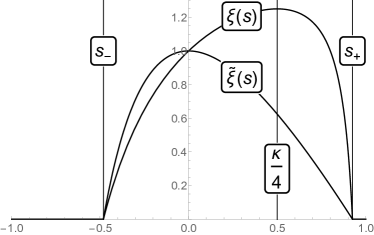
Figure 1.1: Left: A graph of the Hausdorff dimensions $\widetilde{\xi}(s)$ of $\widetilde{\Theta}^{s}(D_{\eta})$ and $\xi(s)$ of $\Theta^{s}(D_{\eta})$ from Theorem 1.1 as $s$ ranges from $-1$ to $1$ for $\kappa=2$. The value of $s$ which maximizes $\widetilde{\xi}$ is $0$ and the value of $s$ which maximizes $\xi$ is $\kappa/4=1/2$. Note that $\xi(\kappa/4)=1+\kappa/8$ which is the almost sure Hausdorff dimension of $\operatorname{SLE}_{\kappa}$ [Bef08]. Right: a graph of the bulk integral means spectrum $\operatorname{IMS}_{D_{\eta}}(a)$ of $D_{\eta}$ from Corollary 1.9 as $a$ ranges from $-7$ to $7$ for $\kappa=3$.

The $\operatorname{SLE}_{\kappa}(\underline{\rho})$ processes are an important variant of $\operatorname{SLE}$ in which one keeps track of extra marked points — so-called force points. The force points can be either on the domain boundary or in its interior and are respectively referred to as boundary and interior force points. These processes were first introduced by Lawler, Schramm, and Werner in [LSW03, Section 8.3] and, just like ordinary $\operatorname{SLE}_{\kappa}$, the $\operatorname{SLE}_{\kappa}(\rho)$ processes naturally arise in many different contexts. Since $\operatorname{SLE}_{\kappa}(\underline{\rho})$ for different vectors of weights $\underline{\rho}$ has the same behavior when it is not interacting with its force points, one expects an analog of Theorem 1.1 to be true for such processes provided we exclude points near the boundary of the domain and stop the path before interacting with an interior force point. Furthermore, by SLE duality, one expects an analog of Theorem 1.1 for $\kappa>4$. Such results do indeed hold true, as described in the following corollary.

Corollary 1.3.

Let $D\subset\mathbf{C}$ be a smoothly bounded domain. Let $\kappa>0$ and let $\underline{\rho}$ be a vector of real weights. Let $\eta$ be a chordal $\operatorname{SLE}_{\kappa}(\underline{\rho})$ process in $D$, with any choice of initial and target points and force points located anywhere in $\overline{D}$, run up until the first time it either hits an interior force point or hits the continuation threshold (c.f. [MS16c, Section 2.1]). Fix $s\in(-1,1)$. Almost surely, the following is true. Let $V$ be a connected component of $D\setminus\eta$ or a connected component of $D\setminus\eta([0,t])$ for any $t>0$ before $\eta$ hits an interior force point or the continuation threshold and let $\phi:\mathbf{D}\rightarrow V$ be a conformal map. Then

$$\dim_{\mathcal{H}}\left(\widetilde{\Theta}^{s}(V)\setminus\phi^{-1}(\partial D)\right) =\dim_{\mathcal{H}}\left(\widetilde{\Theta}^{s;\geq}(V)\setminus\phi^{-1}(\partial D)\right)=\widetilde{\xi}(s),\quad 0\leq s\leq s_{+}$$

$$\dim_{\mathcal{H}}\left(\widetilde{\Theta}^{s}(V)\setminus\phi^{-1}(\partial D)\right) =\dim_{\mathcal{H}}\left(\widetilde{\Theta}^{s;\leq}(V)\setminus\phi^{-1}(\partial D)\right)=\widetilde{\xi}(s),\quad s_{-}\leq s\leq 0$$

$$\dim_{\mathcal{H}}\left(\Theta^{s}(V)\setminus\partial D\right) =\dim_{\mathcal{H}}\left(\Theta^{s;\geq}(V)\setminus\partial D\right)=\xi(s),\quad \frac{\kappa}{4}\leq s\leq s_{+}$$

$$\dim_{\mathcal{H}}\left(\Theta^{s}(V)\setminus\partial D\right) =\dim_{\mathcal{H}}\left(\Theta^{s;\leq}(V)\setminus\partial D\right)=\xi(s),\quad s_{-}\leq s\leq\frac{\kappa}{4}$$

That is, the conclusion of Theorem 1.1 holds a.s. away from the domain boundary at all times simultaneously for an $\operatorname{SLE}_{\kappa}(\underline{\rho})$ with a general $\kappa>0$ and vector of weights $\underline{\rho}$ up until the process either hits an interior force point or the continuation threshold.

Proof.

This follows from Theorem 1.1 combined with Proposition 2.15 below. Note that the functions $\widetilde{\xi}(s)$ and $\xi(s)$ are unaffected if we replace $\kappa$ by $16/\kappa$, as one would expect from SLE duality [Zha08a, Zha10, Dub09a, MS16c, MS13]. ∎

Remark 1.4.

We believe that the techniques developed in this paper could also be employed to describe the multifractal behavior of the $\operatorname{SLE}_{\kappa}(\underline{\rho})$ processes even near their intersection points with the domain boundary and near their tip, though we will not carry this out here.

Roughly speaking, the harmonic measure spectrum of a hull $A\subset\mathbf{H}$ gives, for each $\alpha\in(1/2,\infty)$, the Hausdorff dimension of the set $\Theta^{\alpha}_{\operatorname{hm}}(A)$ of points $x\in\partial A$ for which the harmonic measure from $\infty$ of $B_{\epsilon}(x)$ in $\mathbf{H}\setminus A$ decays like $\epsilon^{\alpha}$ as $\epsilon\rightarrow 0$ (or in the pre-image $\widetilde{\Theta}^{\alpha}_{\operatorname{hm}}(A)$ of $\Theta^{\alpha}_{\operatorname{hm}}(A)$ under a conformal map $\mathbf{D}\rightarrow\mathbf{H}\setminus A$). In [JVL12, Section 2.3], the authors give a rigorous treatment of the harmonic measure spectrum at the tip of a curve. A nearly identical construction works for the harmonic measure spectrum of a whole hull in $\mathbf{H}$. Similar constructions also work for hulls in $\mathbf{D}$ or $\mathbf{C}$. In particular, one has (see [JVL12, Lemma 2.3])

$$\Theta^{s}(A)=\Theta^{\frac{1}{1-s}}_{\operatorname{hm}}(\mathbf{H}\setminus A)\quad\forall s\in(-1,1).$$ (1.7)

Remark 1.5.

In light of the relationship between $\operatorname{SLE}_{6}$ and Brownian motion [LSW01a], we see that Corollary 1.3 with $\kappa=6$ yields the harmonic measure spectrum for the Brownian frontier computed in [Law96, LSW01a, LSW01b, LSW01c, LSW02].

Remark 1.6.

In [Dup00] (see in particular [Dup00, Equation 6]), Duplantier predicts that the harmonic measure spectrum for the bulk of the $\operatorname{SLE}_{\kappa}$ curve is given by

$$f(\alpha)=\alpha+\frac{25-c}{24}\left(1-\frac{1}{2}\left(2\alpha-1+\frac{1}{2\alpha-1}\right)\right),$$ (1.8)

where

$$c=\frac{(6-\kappa)(6-16/\kappa)}{4}$$

is the central charge. The exponent (1.4) is related to the exponent (1.8) by

$$\xi(s)=f\left(\frac{1}{1-s}\right).$$

This is what we would expect in light of (1.7).

The dimension $\xi(s)$ attains a unique maximum value of $1+\kappa/8$ on $[-1,1]$ at $s=\kappa/4$. This maximum value coincides with the Hausdorff dimension of the $\operatorname{SLE}_{\kappa}$ curve [Bef08], which suggests that near a “typical point” of $\eta$, the modulus of the derivative of a conformal map from $D_{\eta}$ to $\mathbf{D}$ grows like $\operatorname{dist}(z,\eta)^{\frac{\kappa}{4-\kappa}}$. Hence Theorem 1.1 gives an alternative proof of the following.

Corollary 1.7.

Let $\kappa\leq 4$. The Hausdorff dimension of an $\operatorname{SLE}_{\kappa}$ curve $\eta$ is a.s. equal to $1+\kappa/8$.

We remark that we believe that the methods that we use to establish the lower bound in Theorem 1.1 could be employed to give an independent derivation of the lower bound of the dimension of $\operatorname{SLE}_{\kappa}$ for all $\kappa>0$, however we will not carry this out here.

1.3 Optimal Hölder exponent for map uniformizing an $\operatorname{SLE}$

Another consequence of Theorem 1.1 is that it is allows us to determine the optimal bulk Hölder exponent for the conformal map which uniformizes the complement of an $\operatorname{SLE}_{\kappa}$ curve. (Note that this result concerns a different problem than [JVL11], which gives the optimal Hölder exponent for the $\operatorname{SLE}_{\kappa}$ curve itself with the capacity parameterization.)

Corollary 1.8.

Suppose that we have the same setup as in Theorem 1.1 and let $\phi\colon{\mathbf{D}}\to D_{\eta}$ be a conformal map taking $-i$ and $i$, respectively, to the start and end points of $\eta$. On any subset of $\mathbf{D}$ lying at positive distance from $\{-i,i\}$, the function $\phi$ is $\alpha$-Hölder continuous for every $\alpha<(1-s_{+})$ and is not $\alpha$-Hölder continuous for every $\alpha>(1-s_{+})$.

Proof.

Suppose that $s>s_{+}$. By Theorem 1.1, $\widetilde{\Theta}^{s;\geq}(D_{\eta})=\emptyset$ a.s. In fact, the proof of Theorem 1.1 gives a slightly stronger statement, namely that for each $\delta>0$, it is a.s. the case that $|\phi^{\prime}(z)|\leq\epsilon^{-s}$ for each sufficiently small $\epsilon>0$ and each $z\in(1-\epsilon)\partial\mathbf{D}$ lying at distance at least $\delta$ from $\{-i,i\}$ (the relation (5.2) from Proposition 5.1 shows this with $\phi$ replaced by the inverse of the centered forward Loewner map for $\eta$ stopped at time $t>0$, and this is easily transferred to $\phi$). Consequently, if $x\in\partial\mathbf{D}$ lies at distance at least $\delta$ from $\{-i,i\}$ then $|\phi^{\prime}(z)|\preceq(1-|z|)^{-s}$ for each $z$ in the line segment $[(1-\epsilon)x,x]$. Integrating this relation gives $|\phi(x)-\phi((1-\epsilon)x)|\preceq\epsilon^{1-s}$. Similarly, if $z,w\in(1-\epsilon)\partial\mathbf{D}$ each lie at distance at least $\delta$ from $\{-i,i\}$, then $|\phi(z)-\phi(w)|\preceq|z-w|\epsilon^{-s}$. Combining these relations with $\epsilon=|x-y|$ and applying the triangle inequality shows that $|\phi(x)-\phi(y)|\preceq|x-y|^{1-s}$ whenever $x,y\in\partial\mathbf{D}$ lie at distance at least $\delta$ from $\{-i,i\}$. This proves the upper bound.

Now suppose $s<s_{+}$. Theorem 1.1 implies that $\widetilde{\Theta}^{s}(D_{\eta})\neq\emptyset$ a.s. Fix $x\in\widetilde{\Theta}^{s}(D_{\eta})$ and for $\epsilon>0$, let $y_{\epsilon}=(1-\epsilon)x$. Then we know that $|\phi^{\prime}(y_{\epsilon})|\succeq\epsilon^{-s+o_{\epsilon}(1)}$. Standard distortion estimates for conformal maps then imply that $|\phi^{\prime}(z)|\succeq\epsilon^{-s+o_{\epsilon}(1)}$ for all $z\in B_{\epsilon/2}(y_{\epsilon})$, which in turn implies that $\phi$ is not $(1-s)$-Hölder continuous. This proves the lower bound. ∎

As explained above in the context of Theorem 1.1, the statement of Corollary 1.8 also applies for $\operatorname{SLE}_{\kappa}$ curves with $\kappa>4$ away from intersections with the domain boundary (by $\operatorname{SLE}$ duality) and for $\operatorname{SLE}_{\kappa}(\underline{\rho})$ curves for all $\kappa>0$, also away from intersection with the domain boundary (by absolute continuity).

1.4 Integral means spectrum

The integral means spectrum of a simply connected domain $D\subset\mathbf{D}$ is the function $\operatorname{IMS}_{D}:\mathbf{R}\rightarrow\mathbf{R}$ defined by

$$\operatorname{IMS}_{D}(a):=\limsup_{\epsilon\rightarrow 0}\frac{\log\int_{\partial B_{1-\epsilon}(0)}|\phi^{\prime}(z)|^{a}\,dz}{-\log\epsilon},$$ (1.9)

where $\phi:\mathbf{D}\rightarrow D$ is a conformal map. (There is a three parameter family of such conformal maps, but $\operatorname{IMS}_{D}(a)$ does not depend on the specific choice of $\phi$.) The integral means spectrum is of substantial interest in complex analysis, primarily in the form of the universal integral means spectrum, which is defined by

$$\operatorname{IMS}^{U}(a):=\sup_{D}\operatorname{IMS}_{D}(a)$$

where the supremum is over all simply connected domains $D\subset\mathbf{C}$. It has been conjectured by Kraetzer [Kra96] that $\operatorname{IMS}^{U}(a)=t^{2}/4$ for $|t|\leq 2$ and $\operatorname{IMS}^{U}(a)=|t|-1$ for $|t|\geq 2$. This conjecture has several important consequences in complex analysis. See, e.g., [Pom97, BS05, HS08, Pom92] for more details. The integral means spectrum is often very difficult to compute in practice for deterministic domains. However, domains bounded by random fractals (e.g. the complement of an $\operatorname{SLE}_{\kappa}$ curve) are sometimes more tractable. For example, in [BS09] Beliaev and Smirnov give an explicit calculation of the average integral means spectrum of the complement of a whole plane $\operatorname{SLE}_{\kappa}$ curve (which is defined as in (1.9) but with $|\phi^{\prime}(z)|^{a}$ replaced by $\mathbf{E}(|\phi^{\prime}(z)|^{a})$).

In this paper we shall be interested in a slight refinement of the definition of the integral means spectrum for the complement of a curve which negates possible pathologies arising from unusual behavior at its endpoints or when it intersects itself or the boundary of the domain. Namely, let $D\subset\mathbf{C}$ be a bounded simply connected domain with smooth boundary and let $\eta:[0,T]\rightarrow\overline{D}$ be a non-self-crossing curve (we allow $T=\infty$). Let $V$ be a connected component of $D\setminus\eta$. Let $x_{V}$ be the first (equivalently last) point of $\partial V$ hit by $\eta$ and let $\phi:\mathbf{D}\rightarrow V$ be a conformal map.

For $\zeta>0$, let

$$I^{\zeta}(\phi):=\phi^{-1}\left(\partial V\setminus(B_{\zeta}(\eta(T))\cup B_{\zeta}(x_{V})\cup B_{\zeta}(\partial D))\right).$$ (1.10)

Let $A_{\epsilon}^{\zeta}(\phi)$ be the set of $z\in\partial B_{1-\epsilon}(0)$ with $z/|z|\in I^{\zeta}(\phi)$. The bulk integral means spectrum of $V$ is the function $\operatorname{IMS}_{V}:\mathbf{R}\rightarrow\mathbf{R}$ defined by

$$\operatorname{IMS}_{V}^{\operatorname{bulk}}(a):=\sup_{\zeta>0}\limsup_{\epsilon\rightarrow 0}\frac{\log\int_{A_{\epsilon}^{\zeta}(\phi)}|\phi^{\prime}(z)|^{a}\,dz}{-\log\epsilon}.$$ (1.11)

One can check that the definition (1.11) does not depend on the choice of $\phi$.

We extract the following from the proof of Theorem 1.1.

Corollary 1.9.

For $a\in\mathbf{R}$ with $a<\frac{(4+\kappa)^{2}}{8\kappa}$, let

$$s_{*}(a):=-1+\frac{4+\kappa}{\sqrt{(4+\kappa)^{2}-8a\kappa}}.$$ (1.12)

Also let $s_{-}$ and $s_{+}$ be as in (1.5) and (1.6) and let $a_{-}$ (resp. $a_{+}$) be the value of $a$ for which $s_{*}(a)=s_{-}$ (resp. $s_{*}(a)=s_{+}$). Set

$$\xi_{\operatorname{IMS}}(a):=\begin{dcases}-1+s_{-}a,\qquad&a<a_{-}\\ -a+\frac{(4+\kappa)(4+\kappa-\sqrt{(4+\kappa)^{2}-8a\kappa})}{4\kappa},\qquad&a\in[a_{-},a_{+}]\\ -1+s_{+}a,\qquad&a>a_{+}.\end{dcases}$$ (1.13)

Suppose we are in the setting of Corollary 1.3. Almost surely, the following is true. Let $a\in\mathbf{R}$ and let $V$ be a complementary connected component of either $D\setminus\eta$ or of $D\setminus\eta^{t}$ for any $t>0$ (before $\eta$ hits an interior force point or the continuation threshold if it is an $\operatorname{SLE}_{\kappa}(\underline{\rho})$ process). Then

$$\operatorname{IMS}_{V}^{\operatorname{bulk}}(a)=\xi_{\operatorname{IMS}}(a).$$ (1.14)

The result of Corollary 1.9 is in agreement with the (rigorously proven) formula for the average bulk integral means spectrum of whole-plane $\operatorname{SLE}$ in [BS09, Theorem 1] for $a\in[a_{-},a_{+}]$, and with [BS09, Conjecture 1] for the a.s. bulk integral means spectrum for all values of $a\in\mathbf{R}$.

Remark 1.10.

As conjectured in [BS09], the a.s. bulk integral means spectrum of Corollary 1.9 differs from the average integral means spectrum computed in [BS09] for values of $a\notin[a_{-},a_{+}]$. We explain why this is the case. First, as noted in [BS09], we expect the average and a.s. bulk integral means spectra to differ because the function which gives the average bulk integral means spectrum does not satisfy Makarov’s [Mak98] characterization of possible integral means spectra. At a more heuristic level, the average integral means spectrum for $a\notin[a_{-},a_{+}]$ is distorted by the occurrence of the small (but still positive) probability event that a conformal map $\phi:\mathbf{D}\rightarrow V$ satisfies $|\phi^{\prime}(z)|\approx(1-|z|)^{-s}$ for some $z$ close to $\partial\mathbf{D}$ and some $s\notin[s_{-},s_{+}]$. However, this event a.s. does not occur in the limit (c.f. Theorem 1.1) so does not affect the a.s. bulk integral means spectrum.

1.5 Outline

There is a systematic approach to computing Hausdorff dimensions of random fractal sets of the sort we consider here. One first gets a sharp estimate for the probability that a single point is contained in the set (the “one-point estimate”) and uses this to get an upper bound on the Hausdorff dimension. One then defines a subset of the set of interest (the “perfect points”) and obtains an estimate for the probability that any two given points are perfect (the “two-point estimate”). This enables one to define a Frostman measure on the set of perfect points and thereby obtain a lower bound on the Hausdorff dimension of the set of interest (see [MP10, Section 4] for more on Frostman measures and their connection to Hausdorff dimension). We will follow this outline here. See, e.g., [MW17, MWW15, JVL12, MSW14] for more examples of this technique.

We will now give a moderately detailed outline of the remainder of this paper. The reader should note that this section does not constitute a precise description of all of the proofs in our paper, but rather is only a heuristic guide. For the sake of brevity, many technical details have been omitted, especially in regards to proof of the two-point estimate.

In Section 2, we will give some background on the objects which appear in our proofs, including SLE, the GFF, and the various couplings between them. We will also establish some notation, introduce the main regularity conditions we will use in our estimates, and prove some elementary lemmas which we will need in the sequel.

Next we will prove our one-point estimate. This is done in two stages. In Section 3, we will establish pointwise derivative estimates for the inverse centered Loewner maps $(f_{t}^{-1})$ for an $\operatorname{SLE}_{\kappa}$. Roughly, our estimates will take the form

$$\mathbf{P}(|(f_{t}^{-1})^{\prime}(z)|\approx\epsilon^{-s},\>\text{regularity conditions})\approx\epsilon^{\alpha(s)},\qquad\forall s\in(-1,1),\qquad\forall z\in\mathbf{H}\>\operatorname{with}\>\operatorname{Im}z=\epsilon,$$ (1.15)

with $\alpha(s)=\frac{(4+\kappa)^{2}s^{2}}{8\kappa(1+s)}$. The proof of these estimates is based on a family of non-negative martingales for the reverse Loewner flow $(g_{t})$, analogous to the martingales for the forward $\operatorname{SLE}_{\kappa}$ flow in [SW05, Section 5]. The reverse Loewner flow is of interest because we have $g_{t}\overset{d}{=}f_{t}^{-1}$ for each fixed $t$ (see, e.g., [RS05, Lemma 3.1]). For a given $z\in\mathbf{H}$ with $\operatorname{Im}z=\epsilon$, one can find a martingale $M_{t}^{z}$ with the property that $M_{t}\mathbf{1}_{\underline{E}(z)}\approx\epsilon^{-\alpha(s)}$, where $\underline{E}(z)$ denotes the event in the probability in (1.15) with $g_{t}$ in place of $f_{t}^{-1}$. We then arrive at

$$\mathbf{P}(\underline{E}(z))\approx\epsilon^{\alpha(s)}\mathbf{P}^{z}_{*}(\underline{E}(z)),$$

where $\mathbf{P}^{z}_{*}$ denotes the measure obtained by re-weighting the law of the original $\operatorname{SLE}_{\kappa}$ process by $M$ (which will be the law of a reverse chordal $\operatorname{SLE}_{\kappa}(\rho)$ for an appropriate $\rho$). Hence we just need to show $\mathbf{P}_{*}^{z}(\underline{E}(z))$ is uniformly positive, independent of $\epsilon$. This is done in two steps. First, to obtain $\mathbf{P}_{*}^{z}(|g_{t}^{\prime}(z)|\approx\epsilon^{-s})\rightarrow 1$ as $\epsilon\rightarrow 0$, we use a coupling of $g_{t}$ with a GFF together with a coordinate change argument similar in spirit to the proof of [MS16e, Theorem 8.1]. To obtain that the auxiliary regularity conditions hold with uniformly positive probability under $\mathbf{P}_{*}^{z}$, we use a combination of stochastic calculus, forward/reverse (in the sense of Loewner flows) SLE symmetry, and GFF coupling arguments.

In Section 4 we use the estimate of Section 3 to establish pointwise derivative estimates for the “time infinity” conformal map $\Psi_{\eta}$ associated with an $\operatorname{SLE}_{\kappa}$ process $\eta$ from $-i$ to $i$ in the unit disk $\mathbf{D}$, defined as follows. Let $D_{\eta}$ be the right connected component of $\mathbf{D}\setminus\eta$, as in Theorem 1.1. Let $\Psi_{\eta}:D_{\eta}\rightarrow\mathbf{D}$ be the unique conformal map fixing $-i$, $i$, and 1. Our estimates for $\Psi_{\eta}$ take the form

$$\mathbf{P}\left(\operatorname{dist}(z,\eta)\approx\epsilon^{1-s},\>|\Psi_{\eta}^{\prime}(z)|\approx\epsilon^{s},\>\text{regularity conditions}\right)\approx\epsilon^{\gamma(s)},\qquad\forall s\in(-1,1),\qquad\forall z\in\mathbf{D}$$ (1.16)

where $\gamma(s)=\alpha(s)-2s+1$ and $\alpha(s)$ as above. The idea of the proof of (1.16) is as follows. First we observe using the Koebe quarter theorem that for each $\epsilon>0$ and each $t>0$, the set of points $\underline{A}_{\epsilon}(t)$ in $\mathbf{D}$ for which the analog of the event of (1.15) with $\mathbf{D}$ in place of $\mathbf{H}$ occurs is (approximately) the image under $f_{t}$ of the set $A_{\epsilon}(t)$ of points in $\mathbf{D}$ for which the event of (1.16) holds with $\Psi_{\eta}$ replaced by $f_{t}$ and $\eta$ replaced by $\eta([0,t])$. Hence the estimate (1.15) together with an elementary change of variables yields $\mathbf{E}(\operatorname{Area}A_{\epsilon}(t))\approx\epsilon^{\gamma(s)}$. We are then left to (a) transfer this area estimate from finite time to infinite time and (b) argue that the probability of the event (1.16) does not depend too strongly on $z$. Both tasks will be accomplished by means of various conditioning arguments which rely crucially on the regularity conditions involved in the estimate (1.15).

In Section 5, we will use the estimates (1.15) and (1.16) to prove upper bounds for the Hausdorff dimensions of the sets $\widetilde{\Theta}^{s;*}(D_{\eta})$ and $\Theta^{s;*}(D_{\eta})$, where $*$ stands for $\geq$ or $\leq$ as well as an upper bound for the bulk integral means spectrum of $D_{\eta}$, as claimed in Corollary 1.9.

Before proving our two-point estimate, we need a modification of the estimate (1.16), which we prove in Section 6. Namely, let $\overline{\eta}$ denote the time reversal of $\eta$, which has the law of a chordal $\operatorname{SLE}_{\kappa}$ from $i$ to $-i$ [Zha08b]. Let $\tau_{\beta}$ (resp. $\overline{\eta}_{\beta}$) be the first time $\eta$ (resp. $\overline{\eta}$) hits the ball of radius $e^{-\beta}$ centered at the origin. Let $\eta^{\tau_{\beta}}=\eta([0,\tau_{\beta}])$, $\overline{\eta}^{\overline{\tau}_{\beta}}=\overline{\eta}([0,\overline{\tau}_{\beta}])$, and let $\phi_{\beta}$ be the conformal map from $\mathbf{D}\setminus(\eta^{\tau_{\beta}}\cup\overline{\eta}^{\overline{\tau}_{\beta}})$ to $\mathbf{D}$ which fixes $-i$, $i$, and 1. Then we will use the one-point estimate (1.16) to show

$$\mathbf{P}\left(|\phi_{\beta}^{\prime}(z)|\approx e^{-\beta q},\>\text{regularity conditions}\right)\approx e^{-\beta\gamma^{*}(q)},\qquad\forall q\in(-1/2,\infty).$$ (1.17)

Here $q=s/(1-s)$ and $\gamma^{*}(q)=\gamma(s)/(1-s)=(q+1)\gamma(q)$, with $\gamma$ as in (1.16).

In Section 7 we prove our two-point estimate. This section contains the most technical, but also the most novel, arguments in the paper; see Section 7.1 for a more detailed outline of this section than the one given here. The estimate (1.17) allows us to break the event that $|\Psi_{\eta}^{\prime}(0)|\approx e^{-n\beta}$ down into several stages and estimate each individually. Indeed, if we apply a conformal map from $\mathbf{D}\setminus(\eta^{\tau_{\beta}}\cup\overline{\eta}^{\overline{\tau}_{\beta}})$ to $\mathbf{D}$ which fixes 0, then the rest of the curve will be mapped to another curve whose law is the same as that of $\eta$ (modulo perturbations of its endpoints, which can be dealt with in various ways). In this manner we can construct two approximately independent events $E_{0,1}$ and $E_{0,2}$ whose intersection is contained in the event $\{|\Psi_{\eta}^{\prime}(0)|\approx e^{-2\beta q}\}$. By iterating this procedure we construct a sequence of approximately independent events $E_{0,j}$ such that $|\Psi_{\eta}^{\prime}(0)|\approx e^{-n\beta q}$ on $E_{n}(0):=\bigcap_{j=1}^{n}E_{0,j}$ and $\mathbf{P}(E_{z,j})\approx e^{-\beta\gamma^{*}(q)}$. We can similarly construct events $E_{z,j}$ and $E_{n}(z)$ for any $z\in\mathbf{D}$ by first mapping $z$ to 0.

For the lower bound on $\dim_{\mathcal{H}}\Theta^{s}(D_{\eta})$, the perfect points will be, roughly speaking, the set of $z\in\mathbf{D}$ for which $E_{n}(z)$ occurs for every $n\in\mathbf{N}$. In order to obtain a lower bound on the Hausdorff dimension of the set of perfect points, we need to estimate the probability that $E_{n}(z)$ and $E_{n}(w)$ both occur for $z,w\in\mathbf{D}$, depending on $|z-w|$. To this end, suppose $|z-w|\approx e^{-\beta k}$. We condition on the event $E_{k}(z)$, corresponding to what happens before we get near $z$ and $w$. After we map out the part of the curve which is grown before the $k$th stage, $z$ and $w$ will be at constant order distance from each other. See Figure 1.2.

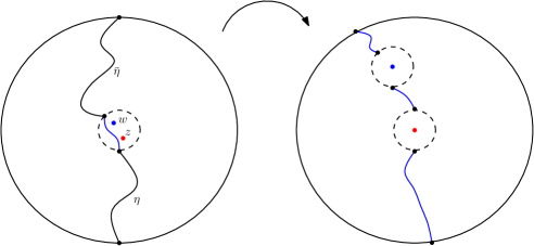
Figure 1.2: If $|z-w|\approx e^{-\beta k}$, then after applying a conformal map which takes the complement of the parts of $\eta$ and $\overline{\eta}$ involved in the event $E_{0}^{k}(z)$ to $\mathbf{D}$ and takes $z$ to 0, the images of $z$ and $w$ will be at constant order distance from each other. Note, however, that in this setting the derivatives of the stage $k+1$-map near $z$ and $w$ are not approximately independent, since they each depend on the whole curve in the picture on the right.

We would like to say that the behaviors of the curve near $z$ and near $w$ are approximately conditionally independent given $E_{k}(z)$. However, the derivatives of the maps we are interested in depend on the whole curve. Hence we need to localize our events. This is accomplished using a different coupling with a GFF, namely the forward SLE/GFF coupling, or “imaginary geometry” coupling studied in [Dub09b, She16, She05, MS16c, MS16d, MS16b, MS13].

At each stage in the construction of the events $E_{n}(z)$, we can add auxiliary curves, which are all flow lines (in the sense of [MS16c]; c.f. Section 2.5) of the same GFF. These auxiliary curves will form pockets surrounding $z$ with the property that the parts of $\eta$ inside different pockets are independent once we condition on the pockets, and the derivative of $\Psi_{\eta}$ at a point inside a pocket can be estimated by the derivative of a map which depends only on the behavior of $\eta$ inside this pocket. We then define the event $E_{z,j}$ so that it depends only on the behavior of the curve inside the $j$th pocket. See Figure 1.3 for an illustration.

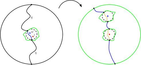
Figure 1.3: A modified version of Figure 1.2 where we add auxiliary curves (shown in green) at each stage to form a pocket. Here we define the events at each stage in terms of only the part of the curve inside the previous pocket. This gives us the needed local independence of the events $E_{z,j}$ and $E_{w,j}$.

The independence of the parts of $\eta$ inside different pockets will eventually enable us to establish the two-point estimate needed for the proof of the lower bounds in Theorem 1.1.

We expect that arguments similar to those in Section 7 may also be useful for proving other estimates for sets related to SLE; see Section 7.6 for further discussion of this point.

In Section 8, we use our two-point estimate to prove lower bounds for the Hausdorff dimensions of the sets $\widetilde{\Theta}^{s}(D_{\eta})$ and $\Theta^{s}(D_{\eta})$ as well as for the bulk integral means spectrum of $D_{\eta}$.

Appendix A contains the proof of an estimate which is needed in Section 3. Appendices B and C contain some technical lemmas which are needed in Sections 6 and 7.

2 Preliminaries

In this section we will establish some notation, give some background on the objects involved in the paper, and prove some elementary lemmas. We recommend that the reader familiarize themselves with Section 2.1 and Section 2.2 before reading the remainder of the paper, as the notation and results of these subsections will be used frequently in the sequel. Sections 2.3, 2.4, and 2.5 contain background on results on SLE, Gaussian free fields, and the couplings between them. Readers who are already familiar with these topics may wish to skim these subsections to acquaint themselves with the notation, and refer back to them as needed. Sections 2.6 and 2.7 contain some elementary lemmas about the sets whose Hausdorff dimensions we will compute. The results of these sections are not used extensively in the sequel, but are needed in Sections 5 and 8. Finally, in Section 2.8, we recall some lemmas from [MW17] which we use frequently throughout the paper.

2.1 Basic notation

Given two variables $a$ and $b$, we say $b=o_{a}(1)$ if $b\rightarrow 0$ as $a\rightarrow 0$ (or as $a\rightarrow\infty$, depending on the context) and we say $b=O_{a}(1)$ if $b$ is bounded above by an $a$-independent constant for sufficiently small (or sufficiently large, depending on context) values of $a$. We usually allow $o_{a}(1)$ and $O_{a}(1)$ terms to depend on certain parameters other than $a$, but not on others. We will describe this dependence as needed.

We say that $a\preceq b$ (resp. $a\succeq b$) if there is a constant $c$ which does not depend on the main parameters of interest such that $a\leq cb$ (resp. $a\geq cb$). We say $a\asymp b$ if $a\preceq b$ and $a\succeq b$. As in the case of $o_{a}(1)$ and $O_{a}(1)$ above, we usually allow the implicit constants in $\preceq,\succeq$, and $\asymp$ to depend on certain parameters, but not on others, and we describe this dependence as needed.

For a point $z\in\mathbf{C}$ and $r>0$, we write $B_{r}(z)$ for the ball of radius $r$ centered at $z$. More generally, for a set $A\subset\mathbf{C}$, we write $B_{r}(A)=\bigcup_{z\in A}B_{r}(z)$.

For a curve $\eta:[0,T]\rightarrow\mathbf{C}$, we will often use the abbreviation

$$\eta^{t}=\eta([0,t]).$$ (2.1)

Furthermore, when there is no risk of ambiguity we will simply write $\eta$ for the entire image of $\eta$.

For a domain $D$ and $z\in D$, we write $\operatorname{hm}^{z}(\cdot;D)$ for the harmonic measure from $z$ in $D$. That is, for $A\subset\partial D$, $\operatorname{hm}^{z}(A;D)$ is the probability that a Brownian motion started from $z$ exits $D$ in $A$.

If $D^{\prime}=D\setminus\eta$ for some non-self-crossing curve $\eta$ in $\overline{D}$ and $z$ is a point on $\eta$ which is visited only once, we will write $z^{-}$ (resp. $z^{+}$) for the prime end of $D^{\prime}$ corresponding to the left (resp. right) side of $z$. When we use this notation, our curve $\eta$ will have an obvious orientation and “left” and “right” are as viewed by someone walking along $\eta$ in the forward direction.

We will also use the following notation.

Notation 2.1.

Given a Jordan domain $D$ and $x,y\in\partial D$, we write $[x,y]_{\partial D}$ for the closed counterclockwise arc from $x$ to $y$ in $\partial D$. We similarly define the open arc $(x,y)_{\partial D}$ and the half-open arcs $(x,y]_{\partial D}$ and $[x,y)_{\partial D}$.

2.2 Reverse continuity conditions

2.2.1 In the upper half plane

Here we introduce a regularity condition which will arise frequently in the remainder of the paper. This regularity event will depend on a certain increasing function (thought of as a modulus of continuity). To lighten notation when referring to such functions, we introduce the following definition.

Definition 2.2.

We denote by $\mathcal{M}$ the set of increasing functions $\mu:(0,\infty)\rightarrow(0,\infty)$ with $\lim_{\delta\rightarrow 0}\mu(\delta)=0$.

Definition 2.3.

Let $f$ be a (random) map from a subdomain $D$ of $\mathbf{H}$ into $\mathbf{H}$. For $\mu\in\mathcal{M}$, let $G(f,\mu)$ be the event that the following occurs. For any $\delta>0$ and any $x,y\in\mathbf{R}\cap\partial D$ with $|x|,|y|\leq\delta^{-1}$ and $|x-y|\geq\delta$, we have $|f(x)|,|f(y)|\leq\mu(\delta)^{-1}$ and $|f(x)-f(y)|\geq\mu(\delta)$.

The statement that $\mathcal{G}(f,\mu)$ holds is the same as the statement that $f^{-1}$ has a certain $\mu$-dependent modulus of continuity on $f(\mathbf{R}\cup\infty)$, with $\mathbf{R}\cup\infty$ given the one-point compactification topology.

We note that

$$G(f,\mu_{1})\cap G(g,\mu_{2})\quad\Rightarrow\quad G(g\circ f,\mu_{2}\circ\mu_{1}).$$ (2.2)

We are interested in the condition $G(f,\mu)$ (and the analogous conditions in the next subsection) for two reasons. The first is that these conditions imply bounds on the distance from certain subsets of $\partial D$ to certain subsets of $\mathbf{R}$ (or $\partial\mathbf{D}$ in the setting of the next subsection) and on the diameter of such subsets (see Lemmas 2.4 and 2.8 below). Such bounds are needed for several purposes in our proofs. One reason is that some of our derivative estimates do not hold if the curve gets too close to the boundary—intuitively, if the curve comes close to hitting the boundary and forming a “bubble”, then the derivative of its associated Loewner map at points inside the bubble will be very small. This manifests itself in the fact that the martingale (3.6) blows up. Another use of such estimates is in checking the hypotheses of the harmonic measure estimates from Appendix B.

The second reason for our interest in $G(f,\mu)$ is as follows. We will often want to study conformal maps which are normalized by specifying the images of certain marked boundary points. When composing various maps, our marked points might be mapped to somewhere other than where we want them to go. So, we will frequently need to apply a conformal automorphism (of $\mathbf{D}$ or $\mathbf{H}$) at the end of our arguments to move the marked points to their desired positions. The condition $G(\cdot,\mu)$ ensures that the images of the marked points are not too close together, and so allows us to control the derivative of this conformal automorphism.

Both of the above uses of our regularity events appear in numerous places throughout the paper.

Lemma 2.4.

Let $\eta$ be a simple curve started from $0$ in $\mathbf{H}$ parameterized by capacity which does not hit $\mathbf{R}$ and recall that $\eta^{t}:=\eta([0,t])$. Let $f_{t}:\mathbf{H}\setminus\eta^{t}\rightarrow\mathbf{H}$ be the centered Loewner maps for $\eta$, i.e. $f_{t}$ is the time $t$ Loewner map for $\eta$, minus a real number chosen so that it maps 0 to 0. Fix $T\in(0,\infty)$ and suppose that for some $\mu\in\mathcal{M}$,

$$f_{T}(-\delta)-f_{T}(0^{-})\leq-\mu(\delta)\quad\operatorname{and}\quad\mu(\delta)\leq f_{T}(\delta)-f_{T}(0^{+}),\qquad\forall\delta>0.$$ (2.3)

Then there is a $\mu^{\prime}\in\mathcal{M}$ and a $d>0$ depending only on $\mu$ and $T$ such that

$$\operatorname{diam}\eta^{T}\leq d\quad\operatorname{and}\quad\text{$\operatorname{Im}z\geq\mu^{\prime}(\delta)$, $\forall\delta>0$, $\forall z\in\eta^{T}$ with $|\operatorname{Re}z|\geq\delta$}.$$ (2.4)

Conversely, if (2.4) holds for some $d>0$ and some $\mu^{\prime}\in\mathcal{M}$, we can find $\mu\in\mathcal{M}$ depending only on $d$ and $\mu^{\prime}$ such that $G(f_{T},\mu)$ holds.

Note that it is clear that $G(f_{T},\mu)$ implies (2.3), so Lemma 2.4 implies in particular that (2.4) holds for some $d$ and $\mu^{\prime}$ depending only on $\mu$ whenever $G(f_{T},\mu)$ occurs.

Proof of Lemma 2.4.

Let $\operatorname{hm}^{\infty}_{T}=\operatorname{hm}^{\infty}(\cdot;\mathbf{H}\setminus\eta^{T})$ denote harmonic measure from $\infty$ in $\mathbf{H}\setminus\eta^{T}$, so for a set $I\subset\partial(\mathbf{H}\setminus\eta^{T})$ (viewed as a collection of prime ends),

$$\operatorname{hm}^{\infty}_{T}I:=\lim_{y\rightarrow\infty}y\mathbf{P}^{iy}(B_{\tau}\in I)$$

for $B$ a Brownian motion and $\tau$ its exit time from $\mathbf{H}\setminus\eta^{T}$. It follows from conformal invariance of Brownian motion that for any $I\subset\partial(\mathbf{H}\setminus\eta^{T})$,

$$\operatorname{hm}^{\infty}_{T}(I)=\frac{1}{\pi}\operatorname{length}f_{T}(I),$$ (2.5)

where by $\operatorname{length}$ we mean Lebesgue measure.

Now, assume (2.3) holds. For any $r>0$ and $x\in\mathbf{R}$, the harmonic measure from $\infty$ in $\mathbf{H}$ of the line segment $[x,x+ir]$ from $x$ to $x+ir$ is a constant depending only on $r$. For $\delta>0$, we can find $r=r(\delta)>0$ such that this constant is $<\pi\mu(\delta)$. If $\eta^{T}$ contains a point $x+iy$ with $x\geq\delta$ and $y\leq r$, then $\operatorname{hm}^{\infty}_{T}([0,\delta])\leq\operatorname{hm}^{\infty}_{T}([x,x+ir])<\pi\mu(\delta)$. This contradicts our hypothesis on (2.3) and the relation (2.5). A similar statement holds if we instead consider $x\leq-\delta$. Hence each point of $\eta^{T}$ with real part $\geq\delta$ in absolute value has imaginary part $\geq r$. This proves the second part of (2.4) with $\mu^{\prime}(\delta)=r$.

For the first part of (2.4), fix $\delta>0$. Denote by $S_{\delta}$ the set of points in $z\in\mathbf{H}$ with $|\operatorname{Re}z|\geq\delta$. By the second part of (2.4),

$$\operatorname{hm}^{\infty}_{T}(\eta^{T}\cap S_{\delta})\leq\frac{1}{\mu^{\prime}(\delta)}\lim_{y\rightarrow\infty}y\mathbf{E}^{iy}\!\left(\operatorname{Im}B_{\tau}\mathbf{1}_{(B_{\tau}\in\eta^{T}\cap S_{\delta})}\right).$$ (2.6)

By [Law05, Proposition 3.38],

$$T=\operatorname{hcap}\eta^{T}=\lim_{y\rightarrow\infty}y\mathbf{E}^{iy}(\operatorname{Im}B_{\tau})$$ (2.7)

so (2.6) is at most $T/\mu^{\prime}(\delta)$. On the other hand, (2.7) and the Beurling estimate imply that $\sup_{z\in\eta^{T}}\operatorname{Im}z$ is bounded above by a constant $C_{0}$ depending only on $T$. The harmonic measure from $\infty$ in $\mathbf{H}$ of $[-\delta,\delta]\times[0,C_{0}]$ is at most a constant $C_{1}$ depending only on $\delta$ and $T$. Therefore

$$\operatorname{hm}^{\infty}_{T}(\eta^{T})\leq T/\mu^{\prime}(\delta)+C_{1}.$$

By [Law05, equation 3.13], this implies $\operatorname{diam}\eta^{T}$ is bounded above by a constant depending only on $\mu$ and $T$.

Conversely, suppose (2.4) holds. For $\delta>0$, let $U_{\delta}$ be the set of points in $z\in\mathbf{H}$ with $|z|\leq d$ and either $|\operatorname{Re}z|\leq\delta/2$ or $\operatorname{Im}z\geq\mu^{\prime}(\delta/2)$. Then $\eta^{T}\subset U_{\delta}$. The harmonic measure from $\infty$ of each sub-interval of $[\delta/2,\delta^{-1}]\cup[-\delta^{-1},-\delta/2]$ in $\mathbf{H}\setminus U_{\delta}$ of length $\delta/2$ is at least some constant $\mu_{0}(\delta)$ depending only on $\delta$ and $\mu^{\prime}(\delta/2)$. By (2.5), this implies that the length of the image of such an interval under $f_{T}$ is at least a $\pi\mu_{0}(\delta)$. On the other hand, [Law05, Proposition 3.46] implies that we can find $\mu_{1}(\delta)>0$ depending only on $\delta$ and $d$ such that $|f_{T}(x)|\leq\mu_{1}(\delta)^{-1}$ for each $x\in[-\delta^{-1},\delta^{-1}]$. This proves that $\mathcal{G}(f_{T},\mu)$ holds with $\mu=(\pi\mu_{0})\vee\mu_{1}$. ∎

2.2.2 In the disk

The following is the analog of Definition 2.3 for the unit disk $\mathbf{D}$.

Definition 2.5.

Let $D\subset\mathbf{D}$ be a subdomain and let $I\subset\partial\mathbf{D}\cap\partial D$. Let $f:D\rightarrow\mathbf{D}$ be a conformal map. Let $\mu\in\mathcal{M}$ (Definition 2.2). We say that $\mathcal{G}_{I}(f,\mu)$ occurs if the following is true. For each $\delta>0$ and each $x,y\in I$ with $|x-y|\geq\delta$, we have $|f(x)-f(y)|\geq\mu(\delta)$. We abbreviate

$$\mathcal{G}(f,\mu)=\mathcal{G}_{\partial\mathbf{D}\cap\partial D}(f,\mu).$$

We also define the following event, which is closely related to $G(f,\mu)$ and is a variant of the condition (2.3).

Definition 2.6.

Let $A\subset\overline{\mathbf{D}}$ be a closed set and $I\subset\overline{\partial\mathbf{D}\setminus A}$. (Oftentimes we will take $I$ to be a closed arc with endpoints in $A$, or a finite union of such arcs.) We say that $\mathcal{G}_{I}^{\prime}(A,\mu)$ occurs if the following is true. For each $\delta>0$, $A$ lies at distance at least $\mu(\delta)$ from $I\setminus B_{\delta}(I\cap A)$. We write

$$\mathcal{G}^{\prime}(A,\mu)=\mathcal{G}_{\overline{\partial\mathbf{D}\setminus A}}(A,\mu).$$

Remark 2.7.

We will frequently find ourselves in the following situation. Suppose we are given a deterministic arc $I\subset\partial\mathbf{D}$, a random closed subset $A\subset\overline{\mathbf{D}}$ with $I\subset\overline{\partial\mathbf{D}\setminus A}$ a.s., and a deterministic $\epsilon>0$. In this case we can find (using monotonicity) a deterministic $\mu\in\mathcal{M}$ for which $\mathbf{P}\!\left(\mathcal{G}_{I}(A,\mu)\right)\geq 1-\epsilon$ where $\mathbf{P}$ is typically the law of SLE.

The conditions of Definitions 2.5 and 2.6 will serve as the main “global regularity” conditions in our estimates starting from Section 4. The relationship between the conditions $\mathcal{G}(\cdot)$ and $\mathcal{G}^{\prime}(\cdot)$ is contained in the following lemma.

Lemma 2.8.

Let $A\subset\overline{\mathbf{D}}$ be a closed set and $I=[x,y]_{\partial\mathbf{D}}$ be an arc contained in $\overline{\partial\mathbf{D}\setminus A}$. Let $m\in(x,y)_{\partial\mathbf{D}}$ and suppose that $|x-m|$ and $|y-m|$ are each at least $\Delta>0$. Let $D$ be the connected component of $\mathbf{D}\setminus A$ containing $I$ on its boundary. Let $\Phi:D\rightarrow\mathbf{D}$ be the unique conformal map taking $x$ to $-i$, $y$ to $i$, and $m$ to $1$.

1. For each $\mu\in\mathcal{M}$, there exists $\mu^{\prime}\in\mathcal{M}$ depending only on $\mu$ and $\Delta$ such that if $\mathcal{G}_{I}(\Phi,\mu)$ occurs, then $\mathcal{G}_{I}^{\prime}(A,\mu^{\prime})$ occurs.

2. Conversely, suppose $I^{\prime}\subset I$ (possibly $I^{\prime}=I$) and $\mathcal{G}_{I^{\prime}}^{\prime}(A,\mu)$ occurs for some $\mu\in\mathcal{M}$. There is a $\mu^{\prime}\in\mathcal{M}$ depending only on $\mu$ and $\Delta$ such that $\mathcal{G}_{I^{\prime}}(\Phi,\mu^{\prime})$ occurs. In fact, the following superficially stronger statement is true. For each $\delta>0$, $\Phi$ is Lipschitz continuous on $I^{\prime}\setminus(B_{\delta}(x)\cup B_{\delta}(y))$ and $\Phi^{-1}$ is Lipschitz continuous on $\Phi(I^{\prime}\setminus(B_{\delta}(x)\cup B_{\delta}(y)))$ with Lipschitz constants depending only on $\mu(\delta)$, $\delta$, and $\Delta$.

Proof.

The basic idea of the proof is similar to that of Lemma 2.4, but we consider harmonic measure from $m$ rather than harmonic measure from $\infty$.

Let $\widehat{D}$ be the radial reflection of $\widehat{D}$ across $I$, viewed as a subset of the Riemann sphere. Extend $\Phi$ to $\widehat{D}$ by Schwarz reflection. Then $\Phi$ maps $\widehat{D}$ into $\mathbf{C}\setminus[i,-i]_{\partial\mathbf{D}}$, and maps $I$ to $[-i,i]_{\partial\mathbf{D}}$.

For $\delta>0$, let $x_{\delta}$ and $y_{\delta}$ be the unique points of $I$ lying at distance $\delta$ from $x$ and $y$, respectively. Also let $\widehat{D}_{\delta}=\widehat{D}\setminus[y_{\delta},y]_{\partial\mathbf{D}}$ and let $\widetilde{y}_{\delta}:=\Phi(y_{\delta})$. Then $\widetilde{y}_{\delta}$ is determined by the condition that the harmonic measure of $[y_{\delta},i]_{\partial\mathbf{D}}$ from $m$ in $\widehat{D}_{\delta}$ equals the harmonic measure of the side of $[\widetilde{y}_{\delta},i]_{\partial\mathbf{D}}$ closer to 0 from 1 in $(\mathbf{C}\cup\infty)\setminus[\widetilde{y}_{\delta},-i]_{\partial\mathbf{D}}$.

If $\mathcal{G}^{*}_{I}(\Phi,\mu)$ occurs, then $\widetilde{y}_{\delta}$ lies at distance at least $\mu(\delta)$ from $i$, which means that the harmonic measure of $[y_{\delta},y]_{\partial\mathbf{D}}$ from 1 in $\widehat{D}_{\delta}$ is at least some constant $\epsilon>0$ depending only on $\mu(\delta)$. By symmetry, the same holds for $[x,x_{\delta}]_{\partial\mathbf{D}}$.

By the Beurling estimate, we can find $\zeta_{0}>0$ depending only on $\epsilon$ such that $\operatorname{dist}(m,A)\geq\zeta_{0}$. We can also find a $\zeta_{1}>0$ such that if $z\in[x_{\delta},y_{\delta}]_{\partial\mathbf{D}}$ lies at distance at least $\zeta_{0}$ from $m$, then the probability that a Brownian motion started from $m$ hits $B_{\zeta_{1}}(z)$ before hitting $[i,-i]_{\partial\mathbf{D}}$ is at most $\epsilon$. If $\operatorname{dist}(z,A)<\zeta_{1}$ for such a $z$, then a Brownian motion started from 1 must hit $B_{\zeta_{1}}(z)$ before hitting either $[y_{\delta},y]_{\partial\mathbf{D}}$ or $[x,x_{\delta}]_{\partial\mathbf{D}}$. Hence we must have $\operatorname{dist}(z,A)\geq\zeta_{1}\wedge\zeta_{0}$ for each $z\in[x_{\delta},y_{\delta}]_{\partial\mathbf{D}}$. This proves assertion 1 with $\mu^{\prime}(\delta)=\zeta_{1}\wedge\zeta_{0}$.

Conversely, suppose $I^{\prime}\subset I$ and $\mathcal{G}_{I^{\prime}}^{\prime}(A,\mu)$ occurs for some $\mu\in\mathcal{M}$. For $\delta>0$ let $x_{\delta}^{\prime}$ be either $x_{\delta}$ (as defined just above) or the endpoint of $I^{\prime}$ closest to $x$, whichever is furthest from $x$. Define $y_{\delta}^{\prime}$ similarly. A Brownian motion started from any point of $[x_{\delta}^{\prime},y_{\delta}^{\prime}]_{\partial\mathbf{D}}$ as a positive probability depending only on $\delta$, $\mu(\delta)$, and $\Delta$ to stay within distance $\mu(\delta)$ of $I$ until it hits $[y_{\delta}^{\prime},y]_{\partial\mathbf{D}}$ (resp. $[x,x_{\delta}^{\prime}]_{\partial\mathbf{D}}$). By the Beurling estimate there is a $\mu^{\prime}(\delta)>0$ depending only on $\mu(\delta)$, $\delta$, and $\Delta$ such that $\Phi([x_{\delta}^{\prime},y_{\delta}^{\prime}]_{\partial\mathbf{D}})$ lies at distance at least $\mu^{\prime}(\delta)$ from $[i,-i]_{\partial\mathbf{D}}$. Thus $\mathcal{G}_{I^{\prime}}(\Phi,\mu^{\prime})$ occurs.

It remains to establish the Lipschitz continuity statement. For this, we observe that for any $z\in[x_{\delta}^{\prime},y_{\delta}^{\prime}]_{\partial\mathbf{D}}$, the Koebe quarter theorem implies

$$\frac{\operatorname{dist}(\Phi(z),[i,-i]_{\partial\mathbf{D}})}{4\operatorname{dist}(z,A)\wedge\delta}\leq|\Phi^{\prime}(z)|\leq\frac{4\operatorname{dist}(\Phi(z),[i,-i]_{\partial\mathbf{D}})}{\operatorname{dist}(z,A)\wedge\delta}.$$

Hence

$$\frac{\mu^{\prime}(\delta)}{8}\leq|\Phi^{\prime}(z)|\leq\frac{8}{\mu(\delta)\wedge\delta}.$$

So, $|\Phi^{\prime}|$ is bounded above and below by positive constants on $[x_{\delta}^{\prime},y_{\delta}^{\prime}]_{\partial\mathbf{D}}$ depending only on $\mu(\delta)$, $\delta$, and $\Delta$ which establishes the desired Lipschitz continuity. ∎

2.3 Schramm-Loewner evolution

Let $t\mapsto W_{t}$ be a continuous function on $[0,\infty)$. The chordal Loewner equation is the ordinary differential equation

$$\partial_{t}g_{t}(z)=\frac{2}{g_{t}(z)-W_{t}},\qquad g_{0}(z)=z.$$ (2.8)

A solution to (2.8) is a family of conformal maps $\{g_{t}:t\geq 0\}$ from subdomains of $\mathbf{H}$ to $\mathbf{H}$, satisfying the hydrodynamic normalization $\lim_{z\rightarrow\infty}(g_{t}(z)-z)=0$. The complements $(K_{t})$ of the domains of $(g_{t})$ in $\mathbf{H}$ are an increasing family of closed subsets of $\mathbf{H}$ called the hulls of the process. The centered Loewner maps corresponding to $(g_{t})$ are defined by

$$f_{t}:=g_{t}-W_{t}.$$

A chordal Schramm-Loewner evolution with parameter $\kappa>0$ ($\operatorname{SLE}_{\kappa}$) is the random evolution obtained by solving (2.8) where the driving process $W$ is $\sqrt{\kappa}$ times a Brownian motion. It can be shown [RS05] that this Loewner evolution is generated by a curve which we typically denote by $\eta$. Chordal $\operatorname{SLE}_{\kappa}$ on other domains is defined by conformal mapping. We refer the reader to [Law05] or [Wer04] for a more detailed introduction to SLE.

More generally, suppose we are given a vector of real weights $\underline{\rho}=(\rho^{1},\ldots,\rho^{n})$ and a collection of points $z^{1},\ldots,z^{n}\in\mathbf{H}$. Chordal $\operatorname{SLE}_{\kappa}(\underline{\rho})$ is the random evolution obtained by solving (2.8) with the driving function $W$ part of the solution to the system of SDE’s

$$dW_{t}=\sqrt{\kappa}dB_{t}+\sum_{i=1}^{n}\operatorname{Re}\frac{\rho^{i}}{W_{t}-V_{t}^{i}}dt,\qquad dV_{t}^{i}=\frac{2}{V_{t}^{i}-W_{t}}dt,\qquad W_{0}=y\qquad V_{0}^{i}=z^{i}.$$ (2.9)

The points $z^{i}$ are called the force points. It is shown in [MS16c] that if the force points are located in $\partial\mathbf{H}$, then the SLE${}_{\kappa}(\underline{\rho})$ curve is a.s. defined and continuous up until the first time it reaches the so-called continuation threshold, i.e., the first time that the sum of the weights of the force points it has either hit or disconnected from its target point is $\leq-2$. By local absolute continuity, the same is true if the curve a.s. does not hit any of its interior force points. The continuity of $\operatorname{SLE}_{\kappa}(\rho)$ for $\rho<-2$ is proved in [MS16a, MSW16]. See [LSW03, SW05, MS16c] for more on $\operatorname{SLE}_{\kappa}(\underline{\rho})$.

We will also need to consider the reverse Loewner equation. This is the ODE

$$\partial_{t}g_{t}(z)=-\frac{2}{g_{t}(z)-W_{t}},\qquad g_{0}(z)=z,$$ (2.10)

whose solution is a family of conformal maps from $\mathbf{H}$ to sub-domains of $\mathbf{H}$. Reverse $\operatorname{SLE}_{\kappa}$ is obtained by taking $W_{t}$ to be $\sqrt{\kappa}$ times a Brownian motion. For each time $t$, the time $t$ centered Loewner map of a reverse $\operatorname{SLE}_{\kappa}$ has the same law as the inverse of the time $t$ centered Loewner map of a forward $\operatorname{SLE}_{\kappa}$ [RS05, Lemma 3.1].

Reverse $\operatorname{SLE}_{\kappa}(\underline{\rho})$ with force points $z^{1},\ldots,z^{n}$ is obtained by solving (2.10) with the driving function $W$ part of the solution to the system of SDE’s

$$dW_{t}=\sqrt{\kappa}dB_{t}+\sum_{i=1}^{n}\operatorname{Re}\frac{\rho^{i}}{W_{t}-V_{t}^{i}}dt,\qquad dV_{t}^{i}=-\frac{2}{V_{t}^{i}-W_{t}}dt,\qquad W_{0}=y\qquad V_{0}^{i}=z^{i}.$$

For a general $\underline{\rho}$ we do not have as simple a relation between forward and reverse $\operatorname{SLE}_{\kappa}(\underline{\rho})$ as we do for ordinary $\operatorname{SLE}_{\kappa}$. However, there are various forward and reverse symmetries, some of which are discussed in [DMS14, She16].

Throughout most of the rest of this paper we will fix $\kappa\in(0,4]$ and we will not always make dependence on $\kappa$ explicit.

2.4 Gaussian free fields

For some of our results, we will make use of couplings of $\operatorname{SLE}_{\kappa}$ with Gaussian free fields. In this section we give some basic background about the latter object.

Let $D$ be a domain in $\mathbf{C}$ with harmonically non-trivial boundary (i.e. a Brownian motion started in $D$ a.s. exits $D$ in finite time). We denote by $H(D)$ the Hilbert space completion of the subspace of $C^{\infty}(\overline{D})$ consisting of those smooth, real-valued functions $f$ such that

$$\int_{D}|\nabla f(z)|^{2}\,dz<\infty,\qquad\int_{D}f(z)\,dz=0$$

with respect to the Dirichlet inner product

$$(f,g)_{\nabla}=\frac{1}{2\pi}\int_{D}\nabla f(z)\cdot\nabla g(z)\,dz.$$ (2.11)

A free-boundary Gaussian free field (GFF) on $D$ is a random distribution (in the sense of Schwartz) on $D$ given by the formal sum

$$h=\sum_{j=1}^{\infty}X_{j}f_{j}$$ (2.12)

where $\{f_{j}\}$ is an orthonormal basis for $H(D)$ and $(X_{j})$ is a sequence of i.i.d. standard Gaussian random variables. It is not defined as a pointwise function, but for each $g\in H(D)$, the formal inner product

$$(h,g)_{\nabla}=\sum_{j=1}^{\infty}(f,g)_{\nabla}$$

converges almost surely. Moreover, $(h,g)$ is a.s. defined for each fixed $g\in L^{2}(D)$ by the formula

$$(h,g)=(h,-\Delta^{-1}g)_{\nabla}$$ (2.13)

where $\Delta^{-1}$ denotes the inverse Laplacian with Neumann boundary conditions. More generally, this formula makes sense if $g$ is any distribution whose inverse Laplacian is in $H(D)$.

Similarly, one can define a zero-boundary GFF on $D$ by replacing $H(D)$ with $H_{0}(D)$, defined as the Hilbert space completion of the space of smooth compactly supported functions on $D$ in the inner product (2.11). A zero boundary GFF is defined without the need to make a choice of additive constant. A Gaussian free field with a given choice of boundary data on $\partial D$ is defined to be a zero boundary GFF plus the harmonic extension of the given boundary data to $D$.

If $V,V^{\perp}\subset H(D)$ are complementary orthogonal subspaces, then the formula (2.12) implies that $h$ decomposes as the sum of its projections onto $V$ and $V^{\perp}$. In particular, we can take $V$ to be the closure $H_{0}(D)$ of $C_{c}^{\infty}(D)$ in the inner product (2.11) and $V^{\perp}$ the set $\operatorname{Harm}_{D}$ of functions in $H(D)$ which are harmonic in $D$. This allows us to decompose a free boundary GFF as the sum of a zero boundary Gaussian free field and a random harmonic function $\mathfrak{h}$ on $D$, the latter defined modulo additive constant. We call these distributions the zero-boundary part and harmonic part of $h$, respectively.

We refer to [She07] and the introductory sections of [SS13] and [MS16e] for more details on GFF’s.

2.4.1 Reverse SLE/GFF coupling

The following relation between free boundary GFFs and reverse $\operatorname{SLE}_{\kappa}(\underline{\rho})$ is established in [She16, Section 4.2]. Let $(g_{t})$ be the centered Loewner maps of a reverse $\operatorname{SLE}_{\kappa}(\underline{\rho})$ with force points $z^{1},\ldots,z^{n}$ as in Section 2.3. Let $h$ be a free boundary GFF on $\mathbf{H}$, independent from $(g_{t})$. For $t\geq 0$ let

$$h_{t}=h\circ g_{t}+\frac{2}{\sqrt{\kappa}}\log|g_{t}(\cdot)|+\frac{1}{2\sqrt{\kappa}}\sum_{i=1}^{n}\rho^{i}G(g_{t}(z^{i}),g_{t}(\cdot)),$$

where

$$G(x,y):=-\log|x-y|-\log|\overline{x}-y|$$

is the Green’s function on $\mathbf{H}$ with Neumann boundary conditions. Let

$$Q=\frac{2}{\sqrt{\kappa}}+\frac{\sqrt{\kappa}}{2}.$$ (2.14)

Let $\tau$ be a stopping time for $\eta$ which is a.s. less than the first time $t$ that $f_{t}(z^{i})=0$ for some $i$. Then [She16, Theorem 4.5] implies that $h_{\tau}+Q\log|g_{\tau}^{\prime}|\overset{d}{=}h_{0}$, modulo additive constant.

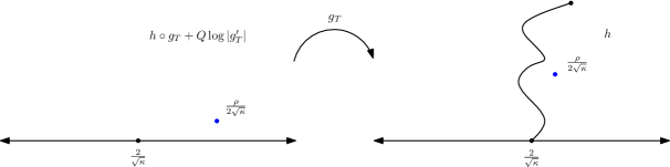
Figure 2.1: An illustration of the reverse SLE/GFF coupling in the case of a single force point (marked in blue). This is the case we will use in Section 3.

There is also an analog of the above coupling for a zero boundary GFF paired with a forward $\operatorname{SLE}_{\kappa}(\underline{\rho})$, which we discuss in Section 2.5.

2.4.2 Estimates for the harmonic part

In the course of proving our one-point estimate we will need some basic analytic lemmas about the harmonic part of a free boundary GFF which we will prove here.

Lemma 2.9.

Let $\mathfrak{h}$ be the harmonic part of a free boundary GFF on $\mathbf{D}$, normalized so that $\mathfrak{h}(0)=0$. Then for any $z,w\in\mathbf{D}$, $\mathfrak{h}(z)$ and $\mathfrak{h}(w)$ are jointly Gaussian with means zero and covariance

$$\mathbf{E}(\mathfrak{h}(z)\mathfrak{h}(w))=-2\log|1-z\overline{w}|.$$

Proof.

For $n\geq 1$, let

$$\phi_{n}(z)=(2/n)^{1/2}\operatorname{Re}z^{n},\qquad\psi_{n}(z)=(2/n)^{1/2}\operatorname{Im}z^{n}.$$ (2.15)

Then $\{\phi_{n},\psi_{n}:n\geq 1\}$ is an orthonormal basis for the set of harmonic functions on $\mathbf{D}$ in the Dirichlet inner product. So, by definition of the free boundary GFF, we can write

$$\sum_{n=1}^{\infty}X_{n}\phi_{n}+\sum_{n=1}^{\infty}Y_{n}\psi_{n},$$ (2.16)

where the $X_{n}$’s and $Y_{n}$’s are i.i.d. $N(0,1)$. From this expression, it follows that $(\mathfrak{h}(z),\mathfrak{h}(w))$ is centered Gaussian for each $z,w\in\mathbf{D}$, and one easily computes

$$\mathbf{E}(\mathfrak{h}(z)\mathfrak{h}(w)) =\sum_{n=1}^{\infty}\phi_{n}(z)\phi_{n}(w)+\sum_{n=1}^{\infty}\psi_{n}(z)\psi_{n}(w)=2\sum_{n=1}^{\infty}\frac{(\operatorname{Re}z^{n})(\operatorname{Re}w^{n})+(\operatorname{Im}z^{n})(\operatorname{Im}w^{n})}{n}$$

$$=\sum_{n=1}^{\infty}\frac{(z\overline{w})^{n}+(w\overline{z})^{n}}{n}=-\log(1-z\overline{w})-\log(1-w\overline{z})=-2\log|1-z\overline{w}|.\qed$$

We also need the following estimate for circle averages of the GFF.

Lemma 2.10.

Let $h$ be a free boundary GFF on $\mathbf{H}$ with additive constant chosen so that its harmonic part vanishes at $a$ for some $a\in\mathbf{H}$. Let $A\subset\mathbf{H}$ be a deterministic hull lying at positive distance from $a$ and let $g:\mathbf{H}\rightarrow\mathbf{H}\setminus A$ be the map which takes some marked point of $a$ to 0 and looks like a translation at $\infty$. Let $\widetilde{h}=h\circ g$ and let $(\widetilde{h}_{\epsilon})$ be the circle average process for $\widetilde{h}$ (see [DS11, Section 3.1] for more on the circle average process). Fix $x\in\mathbf{R}$ and $\xi>1/2$. For any $\delta\geq\epsilon>0$,

$$\mathbf{P}\!\left(|\widetilde{h}_{\epsilon}(x+i\delta)|>(\log\epsilon^{-1})^{\xi}\right)=o_{\epsilon}(\epsilon^{p})\quad\forall p>0,$$ (2.17)

at a rate depending only on $x$, $a$, $\operatorname{diam}A$, $\xi$, and $\delta$, but uniform for $x$ in compact subsets of $\mathbf{R}$, $a$ in compact subsets of $\mathbf{H}$, and $\delta$ in compact subsets of $[\epsilon,\infty)$.

Proof.

Write $h=h^{0}+\mathfrak{h}$, for $h^{0}$ a zero boundary GFF and $\mathfrak{h}$ an independent harmonic function. Let $\mathfrak{h}_{A}$ be the projection of $h^{0}$ onto the set of functions which are harmonic on $\mathbf{H}\setminus A$ and let $h^{0}_{A}=h^{0}|_{A}-\mathfrak{h}_{A}$ be the zero-boundary part of $h^{0}|_{A}$. Then we can write

$$h|_{\mathbf{H}\setminus A}=h^{0}_{A}+\mathfrak{h}_{A}+\mathfrak{h}|_{\mathbf{H}\setminus A},$$ (2.18)

with the three summands independent. The function $g$ increases imaginary parts, so it follows from Lemma 2.9 and a coordinate change to $\mathbf{D}$ that $\mathfrak{h}(g(x+i\delta))$ is centered Gaussian with variance $\leq 2\log\delta^{-1}+O_{\epsilon}(1)$.

By the Koebe distortion theorem, $|g^{\prime}(x+i\delta)|$ is at least a constant depending only on $y$ times $\delta|g^{\prime}(x+iy)|$ for any $y>\delta$. By [Law05, Proposition 3.46] and the Koebe quarter theorem, for large enough $y$ (depending only on $\operatorname{diam}A$), $|g^{\prime}(x+iy)|$ is bounded above by a constant depending only on $\operatorname{diam}A$. By another application of the Koebe quarter theorem, we therefore have

$$\operatorname{dist}(g(x+i\delta),A)\succeq\delta^{2}.$$ (2.19)

It follows from [MS16c, Lemma 6.4] that $\mathfrak{h}_{A}(g(x+i\delta))$ is centered Gaussian with variance at most $2\log\delta^{-1}+O_{\epsilon}(1)$.

By conformal invariance, $h_{A}^{0}\circ g$ has the law of a zero boundary GFF on $\mathbf{H}$. By (2.19) and [DS11, Proposition 3.1], the circle average $(h_{A}^{0}\circ g)_{\epsilon}(x+i\delta)$ is Gaussian with mean 0 and variance at most $2\log\epsilon^{-1}+O_{\epsilon}(1)$. By (2.18),

$$\widetilde{h}_{\epsilon}(x+i\delta)=(h_{A}^{0}\circ g)_{\epsilon}(x+i\delta)+\mathfrak{h}_{A}(g(x+i\delta))+\mathfrak{h}(g(x+i\delta))$$

is Gaussian with mean 0 and variance at most $6\log\epsilon^{-1}+O_{\epsilon}(1)$. We obtain (2.17) from the Gaussian tail bound. ∎

2.5 Imaginary geometry

The proof of the lower bounds in our main theorems will make heavy use of the so-called forward coupling of $\operatorname{SLE}_{\kappa}$ or $\operatorname{SLE}_{\kappa}(\underline{\rho})$ with the GFF with Dirichlet boundary conditions. In this coupling, $\operatorname{SLE}_{\kappa}(\underline{\rho})$ for $\kappa\in(0,4)$ can be interpreted as the flow line of the formal vector field $e^{ih/\chi}$ where $h$ is a GFF and

$$\chi=\frac{2}{\sqrt{\kappa}}-\frac{\sqrt{\kappa}}{2}.$$ (2.20)

For $\kappa>4$, $\operatorname{SLE}_{\kappa}(\underline{\rho})$ can be interpreted as a “tree” or “light-cone” of $\operatorname{SLE}_{16/\kappa}$ flow lines [MS16c]. The case $\kappa=4$ is somewhat degenerate (though simpler to analyze) since $\chi\to 0$ as $\kappa\to 4$. $\operatorname{SLE}_{4}(\underline{\rho})$ has the interpretation of being a level line (rather than a flow line or light cone) of the GFF. See [WW14] for a detailed study of this case.

The coupling of $\operatorname{SLE}_{4}$ with the GFF was actually the first coupling in this family to be discovered [SS13] (see also [SS09] which gives the convergence of the contours of the discrete GFF to $\operatorname{SLE}_{4}$). The existence of the forward coupling in the general setting is established in [Dub09b, SS13, She05, MS16c]; see [MS16c, Theorem 1.1] for a precise statement. The theory of how different flow lines and light cones of the same GFF interact is developed in [MS16c, MS16d, MS16b, MS13]; these works are also where the term “imaginary geometry” is coined. At this point in time, there are several places which contain short “crash courses” on imaginary geometry which are sufficient to understand its usage in this work. We refer the reader to one of [MS16d, Section 2.2], [MS13, Section 2.3], or [MW17, Section 2.2]; [MS16c, Section 1] and [MS13, Section 4] contain many of the main theorem statements in addition to more detailed overviews of the related literature.

2.6 Properties of the multifractal spectrum sets

In this subsection we will prove some elementary deterministic properties of the sets of Section 1.1, as well as a lemma which is relevant to the integral means spectrum. See, e.g., [JVL12, Section 2] for some similar estimates in the setting of the tip multifractal spectrum. Our first lemma tells us that the sets of Section 1.1 are only non-empty in the case $s\in[-1,1]$.

Lemma 2.11.

Let $D\subset\mathbf{C}$ be a simply connected domain and let $\phi:\mathbf{D}\rightarrow D$ be a conformal map. For each $x\in\partial\mathbf{D}$, there is a constant $C>1$ depending only on $\phi$ and $\phi(x)$ but uniform for $\phi(x)$ in compact subsets of $\overline{D}$ such that for each sufficiently small $\epsilon>0$,

$$C^{-1}\epsilon\leq|\phi^{\prime}((1-\epsilon)x)|\leq C\epsilon^{-1}.$$

Proof.

By the Cauchy estimate,

$$|\phi^{\prime}((1-\epsilon)x)|\leq\epsilon^{-1}\sup_{z\in B_{\epsilon}((1-\epsilon)x)}|\phi(z)|$$

which gives the upper bound. For the lower bound, we apply the Koebe distortion theorem. ∎

Next we prove some lemmas which give that the multifractal spectrum sets are invariant under reasonable modifications of the definitions.

Lemma 2.12.

Let $D\subset\mathbf{C}$ be a simply connected domain, $\phi:\mathbf{D}\rightarrow D$ a conformal map, and fix $x\in\partial\mathbf{D}$. Let $\gamma:[0,1]\rightarrow\overline{\mathbf{D}}$ be a simple smooth curve such that $\gamma(0)=x$, $\gamma((0,1])\subset\mathbf{D}$, and $\gamma^{\prime}(0)$ is not tangent to $\partial\mathbf{D}$ at $x$. Then

$$\limsup_{\epsilon\rightarrow 0}\frac{\log|\phi^{\prime}((1-\epsilon)x)|}{-\log\epsilon}=\limsup_{\epsilon\rightarrow 0}\frac{\log|\phi^{\prime}(\gamma(\epsilon))|}{-\log\epsilon}.$$ (2.21)

If one of the limsups is in fact a true limit, then the other is as well.

Proof.

This is a straightforward application of the Koebe distortion theorem. ∎

We next show that the multifractal spectrum depends locally on the domain.

Lemma 2.13.

Let $D$ and $D^{\prime}$ be two simply connected domains in $\mathbf{C}$, bounded by curves, which share a common boundary arc $I$. Let $z$ be a prime end lying in the interior of $I$. Then for each $s\in\mathbf{R}$, we have $z\in\Theta^{s}(D)$ if and only if $z\in\Theta^{s}(D^{\prime})$. The same holds with $\Theta^{s,\geq}(\cdot)$ or $\Theta^{s;\leq}(\cdot)$ in place of $\Theta^{s}(\cdot)$.

Proof.

By comparing $D$ and $D^{\prime}$ to the connected component of $D\cap D^{\prime}$ with $I$ on its boundary, it suffices to consider the case where $D^{\prime}\subset D$. Let $\phi:\mathbf{D}\rightarrow D$ and $\psi:\mathbf{D}\rightarrow D^{\prime}$ be the corresponding conformal maps. We can factor $\phi=\psi\circ\xi$, where $\xi=\psi^{-1}\circ\phi$. Then

$$\phi^{\prime}((1-\epsilon)\phi^{-1}(z))=\psi^{\prime}(\xi((1-\epsilon)\phi^{-1}(z)))\xi^{\prime}((1-\epsilon)\phi^{-1}(z))$$ (2.22)

By Schwarz reflection, $\xi$ extends to be analytic in a neighborhood of $\phi^{-1}(z)$, so $|\xi^{\prime}((1-\epsilon)\phi^{-1}(z))|$ is bounded above and below by positive constants for small $\epsilon$. Let $\gamma(\epsilon)=\xi((1-\epsilon)\phi^{-1}(z))$. Note that $\gamma$ is a simple curve in $\mathbf{D}$ with $\gamma(0)=\psi^{-1}(z)$ and $\gamma^{\prime}(0)=-\xi^{\prime}(\phi^{-1}(z))\phi^{-1}(z)$. Since $\xi$ maps a neighborhood of $\phi^{-1}(z)$ in $\partial\mathbf{D}$ into $\partial\mathbf{D}$, it follows that $\xi^{\prime}(\phi^{-1}(z))$ is a real multiple of $\frac{\xi(\phi^{-1}(z))}{\phi^{-1}(z)}=\frac{\psi^{-1}(z)}{\phi^{-1}(z)}$. Hence $\gamma^{\prime}(0)$ is a real multiple of $\psi^{-1}(z)$. In particular $\gamma$ is not tangent to $\partial\mathbf{D}$ at $\psi^{-1}(z)$ so the stated result follows from Lemma 2.12. ∎

We also record the analog of Lemma 2.13 for the integral means spectrum.

Lemma 2.14.

Let $D$ and $D^{\prime}$ be two bounded Jordan domains in $\mathbf{C}$ and suppose there exists a connected boundary arc $I$ shared by $D$ and $D^{\prime}$. Let $\phi\colon\mathbf{D}\to D$ and $\psi\colon\mathbf{D}\to D^{\prime}$ be conformal maps. Let $J^{\prime}$ be a closed subset of the interior of $I$ and let $J$ be a closed subset of the interior of $J^{\prime}$. For $\epsilon>0$, let $A_{\epsilon}$ be the set of $z\in\partial B_{1-\epsilon}(0)$ with $z/|z|\in\phi^{-1}(J)$ and let $A_{\epsilon}^{\prime}$ be the set of $z\in\partial B_{1-\epsilon}(0)$ with $z/|z|\in\psi^{-1}(J^{\prime})$. Then

$$\limsup_{\epsilon\rightarrow 0}\frac{\log\int_{A_{\epsilon}}|\phi^{\prime}(z)|^{a}\,dz}{-\log\epsilon}\leq\limsup_{\epsilon\rightarrow 0}\frac{\log\int_{A_{\epsilon}^{\prime}}|\psi^{\prime}(z)|^{a}\,dz}{-\log\epsilon}.$$ (2.23)

Proof.

Let $\xi$ be the conformal map from a subdomain of $\mathbf{D}$ to a subdomain of $D^{\prime}\cap D$ which equals $\psi^{-1}\circ\phi$ wherever the latter is defined. By Schwarz reflection $\xi$ extends to a conformal map from a neighborhood of $\phi^{-1}(J^{\prime})$ to a neighborhood of $\psi^{-1}(J^{\prime})$. In particular $|\xi^{\prime}|\asymp 1$ on a neighborhood of $\phi^{-1}(J^{\prime})$, with implicit constants independent of $\epsilon$. By a change of variables, for sufficiently small $\epsilon>0$,

$$\int_{A_{\epsilon}}|\phi^{\prime}(z)|^{a}\,dz\asymp\int_{A_{\epsilon}}|\psi^{\prime}(\xi(z))|^{a}\,dz\asymp\int_{\xi(A_{\epsilon})}|\psi^{\prime}(w)|\,dw.$$ (2.24)

Let $p_{\epsilon}$ be the radial projection from $\mathbf{D}$ onto $\partial B_{1-\epsilon}(0)$. By the above application of Schwarz reflection (and the fact that $J$ is contained in the interior of $J^{\prime}$), for sufficiently small $\epsilon>0$, we have that $p_{\epsilon}$ restricts to a diffeomorphism from $\xi(A_{\epsilon})$ to a subset $\widetilde{A}_{\epsilon}^{\prime}$ of $A_{\epsilon}^{\prime}$. Furthermore, since $|\xi^{\prime}|\asymp 1$ on a neighborhood of $\psi^{-1}(J^{\prime})$, we have $|p_{\epsilon}^{\prime}|\asymp 1$ on $\xi(A_{\epsilon})$ for sufficiently small $\epsilon$, and by the Koebe distortion theorem $|\psi^{\prime}(p_{\epsilon}(w))|\asymp|\psi^{\prime}(w)|$ for $w\in\xi(A_{\epsilon})$ and sufficiently small $\epsilon$. Therefore, a second change of variables yields

$$\int_{\xi(A_{\epsilon})}|\psi^{\prime}(w)|\,dw\asymp\int_{\widetilde{A}_{\epsilon}^{\prime}}|\psi^{\prime}(z)|\,dz\leq\int_{A_{\epsilon}^{\prime}}|\psi^{\prime}(z)|\,dz.$$ (2.25)

We obtain (2.23) by combining (2.24) and (2.25). ∎

2.7 Zero-one laws

In this section we will prove that the multifractal spectrum and integral means spectrum of an $\operatorname{SLE}_{\kappa}(\underline{\rho})$ curve are a.s. deterministic and do not depend on $\underline{\rho}$ or on which complementary component of the curve we consider. These statements will be used to conclude the proofs of our main results in Section 8 once we show that the desired lower bounds on the quantities we are interested in hold with positive probability for one specific type of SLE.

Proposition 2.15.

Let $D\subset\mathbf{C}$ be a smoothly bounded domain. Let $\kappa>0$ and let $\underline{\rho}$ be a vector of real weights. Let $\eta$ be a chordal $\operatorname{SLE}_{\kappa}(\underline{\rho})$ process in $D$, with any choice of initial and target points and force points located anywhere in $\overline{D}$, run up until the first time it either hits an interior force point or hits the continuation threshold after which it is no longer defined (c.f. [MS16c, Section 2.1]). Fix $s\in(-1,1)$. Almost surely, the following is true. Let $V$ be a connected component of $D\setminus\eta$ or a connected component of $\ D\setminus\eta([0,t])$ for any $t>0$ and let $\phi:\mathbf{D}\rightarrow V$ be a conformal map. The Hausdorff dimension of each of the multifractal spectrum sets

$$\Theta^{s}(V)\setminus\partial D,\quad,\Theta^{s;\leq}(V)\setminus\partial D\quad\Theta^{s;\geq}(V)\setminus\partial D,$$

$$\widetilde{\Theta}^{s}(V)\setminus\phi^{-1}(\partial D)\quad\widetilde{\Theta}^{s;\leq}(V)\setminus\phi^{-1}(\partial D)\quad\operatorname{and}\quad\widetilde{\Theta}^{s;\geq}(V)\setminus\phi^{-1}(\partial D)$$

from Section 1.1 is a.s. equal to a deterministic constant which depends only on $\kappa$ and $s$. Furthermore, the a.s. Hausdorff dimensions of the corresponding sets for $\kappa$ and $16/\kappa$ are equal.

Proof.

We will prove the proposition for the sets $\Theta^{s}(V)$ and $\widetilde{\Theta}^{s}(V)$; the statements for the sets with the $\leq$ or $\geq$ are proven similarly. By changing coordinates from $\mathbf{D}$ to $\mathbf{H}$, it suffices to prove the proposition with $\widetilde{\Theta}^{s}(V)$ and $\Theta^{s}(V)$ replaced by

$$\widetilde{\Theta}_{\mathbf{H}}^{s}(V)=\left\{x\in\mathbf{R}:\lim_{\epsilon\rightarrow 0}\frac{\log|\psi^{\prime}(x+i\epsilon)|}{-\log\epsilon}=s\right\}\quad\operatorname{and}\quad\Theta_{\mathbf{H}}^{s}(V)=\psi(\widetilde{\Theta}_{\mathbf{H}}^{s}(V))$$ (2.26)

for $\psi:\mathbf{H}\rightarrow V$ a conformal map. This sill be more convenient since we will be working with chordal SLE_κ.

First consider the case where $D=\mathbf{H}$, $\kappa\leq 4$, and $\eta$ is an ordinary $\operatorname{SLE}_{\kappa}$ process. In this case, the statement of the proposition for a complementary connected component $V$ of $\mathbf{H}\setminus\eta$ follows from the statement for $V=\mathbf{H}\setminus\eta^{t}$ by Lemma 2.13 and countable stability of Hausdorff dimension, so it suffices to prove the statement with $V=\mathbf{H}\setminus\eta^{t}$ for a general choice of $t>0$. This will be deduced from the domain Markov property.

By scale invariance the law of each $\Theta_{\mathbf{H}}^{s}(\mathbf{H}\setminus\eta^{t})$ is independent of $t$. Since the derivative of the conformal map $f_{t/2}$ is bounded above and below by positive (random) constants in a neighborhood of each point of $\eta^{t}\setminus\eta^{t/2}$, we infer that $\Theta_{\mathbf{H}}^{s}(\mathbf{H}\setminus\eta^{t})\setminus\eta^{t/2}=\Theta_{\mathbf{H}}^{s}(\mathbf{H}\setminus f_{t/2}(\eta^{t}\setminus\eta^{t/2}))$.

Since conformal maps preserve Hausdorff dimension of sets in the interior of their domains and by Lemma 2.13, we thus have that the Hausdorff dimension of each $\Theta_{\mathbf{H}}^{s}(\mathbf{D}\setminus\eta^{t})$ is equal to the maximum of $\dim_{\mathcal{H}}\Theta_{\mathbf{H}}^{s}(\mathbf{H}\setminus\eta^{t/2})$ and $\dim_{\mathcal{H}}\Theta_{\mathbf{H}}^{s}(\mathbf{H}\setminus f_{t/2}(\eta^{t}\setminus\eta^{t/2}))$. These latter two sets are independent and identically distributed (by the Markov property of SLE) and their Hausdorff dimensions agree in law with that of $\Theta_{\mathbf{H}}^{s}(\mathbf{H}\setminus\eta^{t})$ (by the scale invariance property noted above). A random variable can be equal to the maximum of two independent random variables with the same law as itself only if it is a.s. constant.

To prove the analogous statement for $\widetilde{\Theta}_{\mathbf{H}}^{s}(\mathbf{H}\setminus\eta^{t})$, we observe that $\dim_{\mathcal{H}}\widetilde{\Theta}_{\mathbf{H}}^{s}(\mathbf{H}\setminus\eta^{t})$ is the maximum of $\dim_{\mathcal{H}}f_{t}^{-1}(\widetilde{\Theta}_{\mathbf{H}}^{s}(\mathbf{H}\setminus\eta^{t})\cap\eta^{t/2})$ and $\dim_{\mathcal{H}}f_{t}^{-1}(\Theta_{\mathbf{H}}^{s}(\mathbf{H}\setminus\eta^{t})\setminus\eta^{t/2})$. By the smoothness of the map $f_{t/2}\circ f_{t}^{-1}$ on $f_{t/2}(\mathbf{H}\setminus\eta^{t/2})$ and of $f_{t}^{-1}$ on $\eta^{t}\setminus\eta^{t/2}$, respectively, these dimensions equal $\dim_{\mathcal{H}}f_{t/2}^{-1}\left(\widetilde{\Theta}_{\mathbf{H}}^{s}(\mathbf{H}\setminus\eta^{t/2})\right)$ and $\dim_{\mathcal{H}}(f_{t}\circ f_{t/2}^{-1})^{-1}\left(\widetilde{\Theta}_{\mathbf{H}}^{s}(\mathbf{H}\setminus f_{t/2}(\eta^{t}\setminus\eta^{t/2}))\right)$, respectively. By the Markov property these latter two quantities are i.i.d., and we conclude as above.

The case when $\kappa\leq 4$ and $\underline{\rho}$ and $D$ are arbitrary follows from the above case, Lemma 2.13, and the local absolute continuity of the laws of SLE${}_{\kappa}(\underline{\rho})$ and SLE_κ away from the boundary. The case for $\kappa>4$ follows from the statement for $16/\kappa<4$ together with Lemma 2.13 and SLE duality (see, e.g. [Zha08a, Zha10, Dub09a, MS16c, MS13]). ∎

For the proof of Corollary 1.9, we will also need the analog of Proposition 2.15 for the integral means spectrum.

Proposition 2.16.

Suppose we are in the setting of Proposition 2.15. Fix $a\in\mathbf{R}$. Almost surely, the following is true. Let $V$ be a complementary connected component of either $D\setminus\eta$ or of $D\setminus\eta^{t}$ for any $t>0$. Then $\operatorname{IMS}^{\operatorname{bulk}}_{V}(a)$ is equal to a deterministic constant which depends only on $\kappa$ and $a$. This deterministic constant is the same if we replace $\kappa$ with $16/\kappa$.

Proof.

The is proven similarly to Proposition 2.15 but with Lemma 2.14 used in place of Lemma 2.13. ∎

2.8 SLE stays close to a fixed curve with positive probability

The paper [MW17] proves several estimates which give that SLE_κ curves have a positive chance of staying in a small “tube” around a deterministic curve until getting close to its endpoint. These estimates will be used frequently throughout the paper, so we re-state these estimates here.

Suppose $\underline{\rho}=(\underline{\rho}^{L};\underline{\rho}^{R})=(\rho^{L}_{l},...,\rho^{L}_{0};\rho^{R}_{0},...,\rho^{R}_{r})$ is a vector of $l+r$ weights with $\rho^{L}_{0},\rho^{R}_{0}>-2$ and let $\eta$ be a chordal SLE${}_{\kappa}(\underline{\rho}^{L};\underline{\rho}^{R})$ from 0 to $\infty$ in $\mathbf{H}$ with force point located at points $x_{l}^{L}<\dots<x_{0}^{L}=0^{-}$ and $0^{+}=x_{0}^{R}<\dots<x_{r}^{R}$. The following is [MW17, Lemma 2.3].

Lemma 2.17.

Let $\epsilon>0$ and let $\gamma:[0,T]\rightarrow\overline{\mathbf{H}}$ be a deterministic simple curve started from 0 which stays in $\mathbf{H}$ after time 0. Let $A_{\epsilon}$ be the $\epsilon$-neighborhood of $\gamma$. Then with positive probability, $\eta$ hits $B_{\epsilon}(\gamma(T))$ before exiting $A_{\epsilon}$.

We will also need the analog of Lemma 2.17 for curves which hit the boundary, which is [MW17, Lemma 2.5].

Lemma 2.18.

Suppose $k\in\{1,...,r-1\}$ with $\overline{\rho}_{k}^{R}:=\sum_{j=1}^{k}\rho_{j}^{R}\in(\kappa/2-4,\kappa/2-2)$, so that $\eta$ can hit $[x_{k}^{R},x_{k+1}^{R}]$. Let $\gamma$ be a simple curve from 0 to a point in $[x_{k}^{R},x_{k+1}^{R}]$ which stays in $\mathbf{H}$ except at its endpoints. Let $\epsilon>0$ and let $A_{\epsilon}$ be the $\epsilon$-neighborhood of $\gamma$. There exists $p=p(\epsilon,\underline{\rho},\kappa,\gamma)>0$ such that the following is true. Suppose $|x_{k+1}^{R}-x_{k}^{R}|\geq\epsilon$ and $|x_{k+1}^{R}|\leq\epsilon^{-1}$. Let $A_{\epsilon}$ be the $\epsilon$-neighborhood of $\gamma$. Then with probability at least $p$, $\eta$ hits $[x_{k}^{R},x_{k+1}^{R}]$ before exiting $A_{\epsilon}$.

Remark 2.19.

Lemma 2.18 can also be used to control the behavior of an $\operatorname{SLE}_{\kappa}(\underline{\rho})$ curve in a bounded domain for all time, as follows. First we observe that the statement of Lemma 2.18 is also valid if the interval $[x_{k}^{R},x_{k+1}^{R}]$ is replaced by a single point which is a.s. hit by $\eta$, with the same proof as in [MW17]. Suppose now for concreteness that we have changed coordinates to $\mathbf{D}$ in such a way that the start and end points of $\eta$ are $-i$ and $i$, respectively, and the vector of weights $\underline{\rho}$ is such that $\eta$ a.s. does not hit the continuation threshold in finite time (so is defined for all time). If we let $f:\mathbf{D}\rightarrow\mathbf{H}$ be a conformal map taking $-i$ to $0$ and $i$ to 1, then by the main result of [SW05], the law of $f(\eta)$ is a certain $\operatorname{SLE}_{\kappa}(\underline{\rho}^{\prime})$ from $0$ to $\infty$ in $\mathbf{H}$, with force points located at 1 and the images of the force points for $\eta$ run until the a.s. finite time at which it hits 1. By applying Lemma 2.18 to $f(\eta)$, we infer that for an appropriate choice of $\underline{\rho}$, $\eta$ has positive probability to stay in the $\epsilon$-neighborhood of a curve from $-i$ to $i$ in $\mathbf{D}$ for all time.

3 One point estimates for the inverse maps

In this section we will prove derivative estimates for the inverse centered Loewner maps of a chordal $\operatorname{SLE}_{\kappa}$ process, which we state just below. Let $\kappa\in(0,4]$. Let $\eta$ be a chordal $\operatorname{SLE}_{\kappa}$ process from $0$ to $\infty$ in $\mathbf{H}$. Let $(f_{t})$ be its centered Loewner maps. For $z\in\mathbf{H}$ with $\operatorname{Im}z=\epsilon$, $u>0$, $s\in(-1,1]$, $c>0$, and $r>0$, let $\underline{E}^{s;u}(z;t)=\underline{E}^{s;u}(z;t,c,r)$ be the event that

$$c^{-1}\epsilon^{-s+u}\leq|(f_{t}^{-1})^{\prime}(z)|\leq c\epsilon^{-s-u}\quad\operatorname{and}\quad\operatorname{Im}f_{t}^{-1}(z)\geq r.$$ (3.1)

Theorem 3.1.

Let $z\in\mathbf{H}$ with $\operatorname{Im}z=\epsilon\in(0,1)$ and $R^{-1}\leq|\operatorname{Re}z|\leq R$ for some $R>1$. Define the event $\underline{E}^{s;u}(z;t)=\underline{E}^{s;u}(z;t,c,r)$ as above and define the exponents

$$\alpha(s)=\frac{(4+\kappa)^{2}s^{2}}{8\kappa(1+s)},\qquad\alpha_{0}(s)=\frac{(4+\kappa)^{2}s(2+s)}{8\kappa(1+s)^{2}}.$$ (3.2)

Also let $G(f_{t},\mu)$ be the event of Definition 2.3. For each $t,c,r>0$, each $\mu\in\mathcal{M}$, each $s\in(-1,1]$, and each $R>1$,

$$\mathbf{P}\left(\underline{E}^{s;u}(z;t)\cap G(f_{t},\mu)\right)\preceq\epsilon^{\alpha(s)-\alpha_{0}(s)u}.$$ (3.3)

Furthermore, for each $r>0$, there exists $t_{*}=t_{*}(r)>0$, such that for each $t\geq t_{*}$, we can find $\mu=\mu(t,r)\in\mathcal{M}$ such that for each $c,u>0$, there exists $\epsilon_{0}=\epsilon_{0}(t,r,c,u)>0$ such that for $\epsilon\in(0,\epsilon_{0}]$,

$$\mathbf{P}\left(\underline{E}^{s;u}(z;t)\cap G(f_{t},\mu)\right)\succeq\epsilon^{\alpha(s)+\alpha_{0}(s)u}.$$ (3.4)

In both (3.3) and (3.4), the implicit constants in $\preceq$ and $\succeq$ depend on the other parameters but not on $\epsilon$, and are uniform for $z\in\mathbf{H}$ with $R^{-1}\leq|\operatorname{Re}z|\leq R$.

Remark 3.2.

The reason for the condition $\operatorname{Im}f_{t}^{-1}(z)\geq r$ in the definition of the event $\underline{E}^{s;u}(z;t)$ is because we are interested in the bulk of the curve, not the behavior near the starting point, so we want to eliminate contributions to $\mathbf{P}\left(c^{-1}\epsilon^{-s+u}\leq|(f_{t}^{-1})^{\prime}(z)|\leq c\epsilon^{-s-u}\right)$ coming from the event that $f_{t}^{-1}(z)$ is near 0. The purpose of the condition $G(f_{t},\mu)$ is as explained in Section 2.2.1.

Remark 3.3.

Estimates similar to Theorem 3.1 can be deduced in a somewhat more efficient manner from the results in [RS05, Section 3] and those of [BS09]. In particular, [RS05, Lemma 3.3] implies the upper bound (3.3) for a restricted range of parameter values and an estimate similar to (3.4) can be deduced from [RS05, Corollary 3.5]. Additionally, a version of Theorem 3.1 for whole-plane SLE can be obtained using the moment estimates of [BS09]. These estimates lead to a.s. upper bounds for the integral means spectrum of SLE and for the dimension of the set $\widetilde{\Theta}^{s}(D_{\eta})\subset\partial\mathbf{D}$ (at least for certain parameter values) via arguments similar to those given in Section 5.1 and 5.3. However, these results do not include the additional regularity conditions on the event in the lower bound of Theorem 3.1, so do not lead to proofs of the lower bounds in Theorem 1.1 and Corollary 1.9. Most of the work in the proof of Theorem 3.1 comes from obtaining a lower bound with these regularity conditions.

The proof of Theorem 3.1 proceeds by way of a martingale re-weighting argument. The upper bound (3.3), explained in Section 3.1, is straightforward, but the lower bound is more involved. For this one has to show that the event $\underline{E}^{s;u}(z;t)\cap G(f_{t},\mu)$ holds with uniformly positive probability under the law when we re-weight by our martingale. It is shown in Section 3.8 that the main derivative condition in (3.1) holds with high probability under this weighted law using a coupling with the GFF and a coordinate change trick reminiscent of arguments in [MS16e, Section 8] (we expect that this can also be proven via a longer argument which does not involve the GFF, but we do not carry out such an argument here). To check that the auxiliary conditions hold with uniformly positive re-weighted probability, we use a rather involved stochastic calculus argument which is mostly given in Appendix A.

3.1 Reverse SLE martingales and upper bound

Let $(g_{t})$ be the centered Loewner maps of a reverse $\operatorname{SLE}_{\kappa}$ flow, so

$$dg_{t}(z)=-\frac{2}{g_{t}(z)}\,dt-dW_{t},\qquad g_{0}(z)=z$$ (3.5)

for $W_{t}=\sqrt{\kappa}B_{t}$ and $(B_{t})$ a standard linear Brownian motion. Our interest in $(g_{t})$ stems from the fact that if $(f_{t})$ is as in Theorem 3.1, then $g_{t}\overset{d}{=}f_{t}^{-1}$ for each $t$ (see, e.g. [RS05, Lemma 3.1]).

Let $K_{t}=\mathbf{H}\setminus g_{t}(\mathbf{H})$ be the hulls corresponding to $(g_{t})$. Since $f_{t}^{-1}\overset{d}{=}g_{t}$ for each $t$, it is only a minor abuse of notation to replace $f_{t}^{-1}$ with $g_{t}$ in the definition of the events of Theorem 3.1, and we do so in the remainder of this section.

3.1.1 Reverse SLE martingales

We state here a result originally due to Lawler [Law09, Proposition 2.1], but in a form which is more convenient for our purposes.

Lemma 3.4.

Let $\kappa>0$. Let $(g_{t})$ be as above, $\rho\in\mathbf{R}$, $z\in\mathbf{H}$, and

$$M_{t}^{z}=|g_{t}^{\prime}(z)|^{\tfrac{(8+2\kappa-\rho)\rho}{8\kappa}}(\operatorname{Im}g_{t}(z))^{-\tfrac{\rho^{2}}{8\kappa}}|g_{t}(z)|^{\rho/\kappa}.$$ (3.6)

Then $M_{t}^{z}$ is a martingale. Let $\mathbf{P}_{*}^{z}$ be the law of $(g_{t})$ weighted by $M^{z}$. The law of $(g_{t})$ under $\mathbf{P}_{*}^{z}$ is that of the centered Loewner maps of a reverse $\operatorname{SLE}_{\kappa}(\rho)$ with a force point at $z$. That is, under the reweighted law,

$$dW_{t}=-\operatorname{Re}\frac{\rho}{g_{t}(z)}\,dt+\sqrt{\kappa}dB_{t}^{z}$$ (3.7)

for $B_{t}^{z}$ a $\mathbf{P}_{*}^{z}$-Brownian motion.

Remark 3.5.

The martingale (3.6) is the reverse SLE analog of the local martingale of [SW05, Section 5] in the case of a single force point.

3.1.2 Proof of the upper bound

In this subsection we will prove (3.3) of Theorem 3.1. We will actually prove something a little stronger which is needed to get an upper bound for the dimensions of the sets $\Theta^{s;\leq}(D_{\eta})$ and $\Theta^{s;\geq}(D_{\eta})$ from Section 1.1.

Proposition 3.6.

Let $\alpha(s)$ be as in (3.2) and let $(g_{t})$ be the centered Loewner maps of a reverse $\operatorname{SLE}_{\kappa}$ as above. Fix $c,d>0$. For $s\in[0,1]$, a time $t>0$, and $z\in\mathbf{H}$ with $\operatorname{Im}z=\epsilon\in(0,1)$, let

$$\underline{E}^{s;\infty}(z;t)=\underline{E}^{s;\infty}(z;t,c,d):=\begin{dcases}&\left\{|g_{t}^{\prime}(z)|\geq c^{-1}\epsilon^{-s},\,|g_{t}(z)|\geq d^{-1}\right\},\quad\text{if}\>s\in[0,1]\\ &\left\{|g_{t}^{\prime}(z)|\leq c\epsilon^{-s},\,|g_{t}(z)|\leq d^{-1}\right\},\quad\text{if}\>s\in(-1,0).\end{dcases}$$

For any bounded stopping time $\tau$ for $(g_{t})$,

$$\mathbf{P}\left(\underline{E}^{s;\infty}(z;\tau)\right)\preceq\epsilon^{\alpha(s)}.$$ (3.8)

For any $R>1$, the implicit constant in (3.8) is uniform for $z\in\mathbf{H}$ with $R^{-1}\leq|\operatorname{Re}z|\leq R$.

The estimate (3.3) is immediate from Proposition 3.6 in the case $s\in[0,1]$. To extract (3.3) from Proposition 3.6 in the case $s\in(-1,0)$, we observe that Lemma 2.4 implies that $\operatorname{diam}K_{t}$ is bounded by a constant depending only on $t$ and $\mu$ on the event $G(g_{t}^{-1},\mu)$ (c.f. the discussion following Definition 2.3). For $R^{-1}\leq|\operatorname{Re}z|\leq R$, [Law05, eqn. 3.14] then implies that $|g_{t}(z)|$ is bounded by a constant depending only on $t,\mu$, and $R$ on $\underline{E}^{s;u}(z;t)\cap G(g_{t}^{-1},\mu)$. Thus $\underline{E}^{s;u}(z;t)\cap G(g_{t}^{-1},\mu)\subset\underline{E}^{s+u;\infty}(z;t,c,d)$ for a suitable choice of $d$.

Proof of Proposition 3.6.

This is a standard martingale re-weighting argument. Throughout, we fix $R>1$ and require all implicit constants to be uniform for $z\in\mathbf{H}$ with $R^{-1}\leq|\operatorname{Re}z|\leq R$. Let

$$\rho=\rho(s):=\frac{(4+\kappa)s}{1+s}.$$ (3.9)

and denote by $\mathbf{P}_{*}^{z}$ the law of $(g_{t})$ re-weighted by the martingale of Lemma 3.4 with this choice of $\rho$. By the Loewner equation, $\operatorname{Im}g_{\tau}(z)$ is bounded above by a constant depending only on the essential supremum of $\tau$. Therefore,

$$M_{\tau}^{z}\mathbf{1}_{\underline{E}^{s;\infty}(z;\tau)}\succeq\epsilon^{\tfrac{-s(8+2\kappa-\rho)\rho}{8\kappa}}\mathbf{1}_{\underline{E}^{s;\infty}(z;\tau)}$$ (3.10)

(we can replace the $\succeq$ with an $\asymp$ if we assume that $\operatorname{Im}g_{t}(z)$ is bounded below and $|g_{t}(z)|$ is bounded above). Furthermore, if $R^{-1}\leq|\operatorname{Re}z|\leq R$ then

$$M_{0}^{z}\asymp\epsilon^{-\tfrac{\rho^{2}}{8\kappa}}.$$ (3.11)

Thus the optional stopping theorem implies

$$\epsilon^{\tfrac{-s(8+2\kappa-\rho)\rho}{8\kappa}}\mathbf{P}(\underline{E}^{s;\infty}(z;\tau))\asymp\mathbf{E}\left(M_{\tau}^{z}\mathbf{1}_{\underline{E}^{s;\infty}(z;\tau)}\right)\preceq\epsilon^{-\rho^{2}/8\kappa}\mathbf{P}_{*}^{z}(\underline{E}^{s;\infty}(z;\tau)).$$

Therefore

$$\mathbf{P}(\underline{E}^{s;\infty}(z;\tau))\preceq\epsilon^{\tfrac{s(8+2\kappa-\rho)\rho}{8\kappa}-\tfrac{\rho^{2}}{8\kappa}}\mathbf{P}_{*}^{z}(\underline{E}^{s;\infty}(z;\tau)).$$ (3.12)

The value of the exponent on the right is maximized by taking $\rho=\rho(s)$, as in (3.9). Choosing this value of $\rho$ yields the upper bound (3.8). ∎

3.2 Reduction of the lower bound to a result for a stopping time

Now we turn our attention to the lower bound (3.4) in Theorem 3.1. We continue to assume that we have replaced $f_{t}^{-1}$ with $g_{t}$ in the definition of the events of Theorem 3.1, as in Section 3.1.

Let $T_{r}^{z}$ be the first time $t$ that $\operatorname{Im}g_{t}(z)\geq r$ and fix a time $\overline{t}>0$. Put

$$\tau=\tau_{r}^{z}:=T_{r}^{z}\wedge\overline{t},$$ (3.13)

so that up to an event of probability zero,

$$\{\tau<\overline{t}\}=\{\operatorname{Im}g_{\tau}(z)\geq r\}=\{\operatorname{Im}g_{\overline{t}}(z)\geq r\}.$$

We claim that to prove that (3.4) holds with $\overline{t}$ in place of $t$, and hence to finish the proof of Theorem 3.1, it is enough to prove the following statement.

Proposition 3.7.

Let $\rho=\rho(s)$ be as in (3.9). Let $\mathbf{P}_{*}^{z}$ be the law of a reverse $\operatorname{SLE}_{\kappa}(\rho)$ process $(g_{t})$ with hulls $(K_{t})$, with an interior force point located at $z\in\mathbf{H}$ with $\operatorname{Im}z=\epsilon$. Let $\tau=\tau_{r}^{z}$ be as in (3.13). Define the events $\underline{E}^{s;u}(z;\tau)$ as in (3.1), but with $(g_{t})$ in place of $(f_{t})$ and the time $\tau$ hull $K_{\tau}$ for $(g_{t})$ in place of $\eta^{\tau}$. For each $R>1$ there exists $r_{*}>0$ such that for each $r\geq r_{*}$, we can find $\mu\in\mathcal{M}$ and $t_{*}>0$ such that for each $u>0$ there exists $\epsilon_{0}>0$ such that for each $z\in\mathbf{H}$ with $\operatorname{Im}z=\epsilon\leq\epsilon_{0}$ and $R^{-1}\leq|\operatorname{Re}z|\leq R$ and each $\overline{t}\geq t_{*}$,

$$\mathbf{P}_{*}^{z}\left(\underline{E}^{s;u}(z;\tau)\cap G(g_{\tau}^{-1},\mu)\right)\succeq 1.$$ (3.14)

Here the implicit constant is independent of $\epsilon$ and uniform for $z$ with $R^{-1}\leq|\operatorname{Re}z|\leq R$ (but may depend on $r$, $R$, $\mu$, $\overline{t}$, $u$, and $s$).

We will prove Proposition 3.7 in the subsequent subsections. In the remainder of this subsection we deduce Theorem 3.1 from Proposition 3.7. To lighten notation, in what follows we write $\tau=\tau_{r}^{z}$.

First we note that the probability of the event of Theorem 3.1 is decreasing in $r$, so it suffices to prove (3.4) for $r\geq r_{*}$, with $r_{*}$ as in Proposition 3.7. Observe that $|g_{\tau}(z)|$ is a.s. bounded above by a positive constant on the event $\underline{E}^{s;u}(z;\tau)\cap\mathcal{G}(g_{\tau}^{-1},\mu)$ (c.f. Section 3.1). By combining this with the definition of $\underline{E}^{s;u}(z;\tau)$ we see that

$$M_{\tau}^{z}\mathbf{1}_{\underline{E}^{s;u}(z;\tau)\cap\mathcal{G}(g_{\tau}^{-1},\mu)}\preceq\epsilon^{\tfrac{-(s+u)(8+2\kappa-\rho)\rho}{8\kappa}}\mathbf{1}_{\underline{E}^{s;u}(z;\tau)\cap G(g_{\tau}^{-1},\mu)}.$$

By (3.11) and our choice (3.9) of $\rho$,

$$\epsilon^{\alpha(s)+\alpha_{0}(s)u}\mathbf{P}_{*}^{z}\left(\underline{E}^{s;u}(z;\tau)\cap G(g_{\tau}^{-1},\mu)\right)\preceq\mathbf{P}\left(\underline{E}^{s;u}(z;\tau)\cap G(g_{\tau}^{-1},\mu)\right).$$ (3.15)

Assuming that Proposition 3.7 holds, (3.15) implies (3.4) with $\tau$ in place of $t$. To get the desired bound at the deterministic time $\overline{t}$, for $t\geq\tau$ let $g_{\tau,t}$ be the conformal map defined on $\mathbf{H}$ which satisfies $g_{\tau,t}\circ g_{\tau}=g_{t}$. By the strong Markov property the conditional law given $\{g_{t}\,:\,t\leq\tau\}$ of the family of conformal maps $\{g_{\tau,v+\tau}\,:\,v\geq 0\}$ is the same as the law of the $\{g_{v}\,:\,v\geq 0\}$. For $w\in\mathbf{C}$, $\mu^{\prime}\in\mathcal{M}$ and $C>1$, let $F=F_{\tau,\overline{t}}(w;C,\mu^{\prime})$ be the event that the following is true.

1. $C^{-1}\leq|g_{\tau,t}^{\prime}(w)|\leq C$ for each $t\in[\tau,\overline{t}]$.

2. $G(g_{\tau,\overline{t}}^{-1},\mu^{\prime})$ occurs.

If $C$ is chosen sufficiently large and $\mu^{\prime}\in\mathcal{M}$ is chosen sufficiently small, depending on $\overline{t}$ but uniform for $w$ in compact subsets of $\mathbf{H}$, then $\mathbf{P}(F)$ is at least a positive constant depending uniformly on $w$ in compact subsets of $\mathbf{H}$. Furthermore, since we have a bound on $\operatorname{diam}K_{\tau}$ on the event $\underline{E}^{s;u}(z;\tau)\cap G(g_{\tau}^{-1},\mu)$ (see Lemma 2.4), it follows from the Markov property that

$$\mathbf{P}\left(F\cap\underline{E}^{s;u}(z;\tau)\cap G(g_{\tau}^{-1},\mu)\right)\succeq\mathbf{P}\left(\underline{E}^{s;u}(z;\tau)\cap G(g_{\tau}^{-1},\mu)\right).$$

On the other hand, the definition of $F$ implies that

$$F\cap\underline{E}^{s;u}(z;\tau)\cap G(g_{\tau}^{-1},\mu)\subset\underline{E}^{s;u}(z;\overline{t},c^{\prime},r)\cap G(g_{\overline{t}}^{-1},\mu\circ\mu^{\prime})$$

for some $c^{\prime}>0$ depending on the other parameters (here we use that $\operatorname{Im}g_{t}(z)$ is increasing in $t$ for the condition involving $r$). By making $c$ sufficiently small, we can make $c^{\prime}$ as small as we like. We conclude that (3.4) with $\tau$ in place of implies (3.4) with $\overline{t}$ in place of $t$.

Thus to prove Theorem 3.1 it remains to prove Proposition 3.7. The proof is separated into two major steps: first we prove that the derivative condition in the definition of $\underline{E}^{s;u}(z)$ holds at time $\tau$ with $\mathbf{P}_{*}^{z}$-probability tending to 1 as $\epsilon=\operatorname{Im}z\rightarrow 0$. This is done in Section 3.3 via a coupling with a Gaussian free field. Then we prove that $\mathbf{P}_{*}^{z}\left(\{\tau<\overline{t}\}\cap G(g_{\tau}^{-1},\mu)\right)$ is uniformly positive for sufficiently small $\mu$ and sufficiently large $\overline{t}$. This is done in Appendix A via a stochastic calculus argument.

3.3 Derivative estimate via reverse SLE/GFF coupling

Assume we are in the setting of Proposition 3.7. In this subsection we will prove that $|g_{\tau}^{\prime}(z)|\approx\epsilon^{-s}$ with high probability under $\mathbf{P}_{*}^{z}$. Throughout this subsection, we fix $R>1$, $c>0$, $r>0$, $\mu\in\mathcal{M}$, $\overline{t}>0$, and $z\in\mathbf{H}$ with $\operatorname{Im}z=\epsilon$ and require all implicit constants to be independent of $\epsilon$ and uniform for $R^{-1}\leq|\operatorname{Re}z|\leq R$ and all $o_{\epsilon}(1)$ errors to be uniform for $R^{-1}\leq|\operatorname{Re}z|\leq R$. These quantities are, however, allowed to depend on $R$, $c$, $r$, $\mu$, $\overline{t}$, $s$, and $u$.

Proposition 3.8.

In the setting of Proposition 3.7,

$$\mathbf{P}_{*}^{z}\left(\{|g_{\tau}^{\prime}(z)|\notin[c^{-1}\epsilon^{-s+u},c\epsilon^{-s-u}]\}\cap G(g_{\tau}^{-1},\mu)\cap\{\tau<\overline{t}\}\right)=o_{\epsilon}(1).$$ (3.16)

We prove Proposition 3.8 using a coupling with a Gaussian free field (we expect that one could also do this without using the GFF—perhaps via a longer argument).

Let $h$ be a free boundary GFF on $\mathbf{H}$, independent from $(g_{t})$, normalized so that its harmonic part $\mathfrak{h}$ vanishes at $iy$ for some $y>0$ (which we will specify below in such a way that it depends on $\overline{t}$, but not $\epsilon$). Let $\mathbf{P}_{h}$ be the law of $h$. For $t\geq 0$ let

$$h_{t}=h\circ g_{t}+\frac{2}{\sqrt{\kappa}}\log|g_{t}(\cdot)|+\frac{\rho}{2\sqrt{\kappa}}G(g_{t}(z),g_{t}(\cdot)),$$ (3.17)

where

$$G(x,y):=-\log|x-y|-\log|\overline{x}-y|$$

is the Green’s function on $\mathbf{H}$ with Neumann boundary conditions.

Let $\tau$ be as in (3.13). By [She16, Theorem 2.5], $h_{\tau}+Q\log|g_{\tau}^{\prime}|\overset{d}{=}h_{0}$, modulo additive constant, where $Q=\frac{2}{\sqrt{\kappa}}+\frac{\sqrt{\kappa}}{2}$ is as in (2.14). Let $b_{\tau}$ be this additive constant, so

$$h_{\tau}+Q\log|g_{\tau}^{\prime}|-b_{\tau}\overset{d}{=}h_{0}.$$ (3.18)

The idea of the proof of (3.7) is to estimate the terms other than $\log|g_{\tau}^{\prime}|$ in (3.18), and thereby obtain an estimate for $|g_{\tau}^{\prime}|$. See the proof of [MS16e, Theorem 8.1] for another argument using a similar idea.

Let

$$\widetilde{h}_{0}=h_{\tau}+Q\log|g_{\tau}^{\prime}|-b_{\tau}$$ (3.19)

so that by (3.18), $\widetilde{h}_{0}\overset{d}{=}h_{0}$. Rearranging the definition of $\widetilde{h}_{0}$ gives

$$Q\log|g_{\tau}^{\prime}(w)|=\widetilde{h}_{0}-h_{\tau}+b_{\tau}$$

$$\quad=\widetilde{h}-h\circ g_{\tau}+\frac{2}{\sqrt{\kappa}}\log\frac{|w|}{|g_{\tau}(w)|}+\frac{\rho}{2\sqrt{\kappa}}\left(\log\frac{|g_{\tau}(w)-g_{\tau}(z)|}{|w-z|}+\log\frac{|g_{\tau}(w)-\overline{g_{\tau}(z)}|}{|w-\overline{z}|}\right)+b_{\tau},$$ (3.20)

where here $\widetilde{h}$ is a field with the same law as $h$ and we use $w$ instead of $\cdot$ as a dummy variable. Since all of the non-GFF terms in (3.3) are harmonic away from $z$, the equation still holds for $w\not=z$ if we replace $\widetilde{h}$ and $h\circ g_{\tau}$ with the circle average processes $\widetilde{h}_{\epsilon}$ and $(h\circ g_{\tau})_{\epsilon}$ for these two fields. We will use (3.3) to estimate $b_{\tau}$ and then to estimate $|g_{\tau}^{\prime}(z)|$.

Lemma 3.9.

Let $\xi>1/2$. If $y$ is chosen sufficiently large (independently of $\epsilon$ and uniform for $R^{-1}\leq|\operatorname{Re}z|\leq R$) then

$$(\mathbf{P}_{*}^{z}\otimes\mathbf{P}_{h})\left(\{|b_{\tau}|>(\log\epsilon^{-1})^{\xi}\}\cap G(g_{\tau}^{-1},\mu)\cap\{\tau<\overline{t}\}\right)=o_{\epsilon}(1).$$ (3.21)

Proof.

If we replace the GFF terms with circle averages in (3.3) and evaluate at $w=iy$, we get

$$Q\log|g_{\tau}^{\prime}(iy)| =\widetilde{h}_{\epsilon}(iy)-(h\circ g_{\tau})_{\epsilon}(iy)+\frac{2}{\sqrt{\kappa}}\log\frac{y}{|g_{\tau}(iy)|}$$

$$+\frac{\rho}{2\sqrt{\kappa}}\left(\log\frac{|g_{\tau}(iy)-g_{\tau}(z)|}{|iy-z|}+\log\frac{|g_{\tau}(iy)-\overline{g_{\tau}(z)}|}{|iy-\overline{z}|}\right)+b_{\tau}.$$ (3.22)

By Lemma 2.4 $\operatorname{diam}K_{\tau}\preceq 1$ on $G(g_{\tau}^{-1},\mu)$. By [Law05, Proposition 3.46], $\operatorname{Im}g_{\tau}(iy)\asymp|g_{\tau}(iy)|\asymp 1$ on $G(g_{\tau}^{-1},\mu)$. By the Koebe quarter theorem we also have $|g_{\tau}^{\prime}(iy)|\asymp 1$ on $G(g_{\tau}^{-1},\mu)$ provided $y$ is chosen sufficiently large, depending only on $\mu$, $\overline{t}$, and $R$. Hence each of the terms in (3.3) except for $b_{\tau}$ and the two circle averages is $\asymp 1$ on $G(g_{\tau}^{-1},\mu)\cap\{\tau<\overline{t}\}$ (implicit constants also depending on $y$) if $y$ is chosen sufficiently large, depending only on $\mu$, $\overline{t}$, and $R$. By Lemma 2.10, for $\xi>1/2$,

$$(\mathbf{P}_{*}^{z}\otimes\mathbf{P}_{h})\left(|\widetilde{h}_{\epsilon}(iy)-(h\circ g_{\tau})_{\epsilon}(iy)|>(\log\epsilon)^{\xi}\right)=o_{\epsilon}(1).$$

Note that we took $A=\emptyset$ in that lemma to estimate $\widetilde{h}_{\epsilon}(iy)$ and we took $A=K_{\tau}$ and used that $K_{\tau}$ is independent of $h$ to estimate $(h\circ g_{\tau})_{\epsilon}(iy)$. By re-arranging (3.3) we conclude. ∎

Proof of Proposition 3.8.

Since the circle average process is continuous [DS11, Proposition 3.1], we can take the limit as $w\rightarrow z$ in (3.3) to get

$$Q\log|g_{\tau}^{\prime}(z)| =\widetilde{h}_{\epsilon}(z)-(h\circ g_{\tau})_{\epsilon}(z)+\frac{\rho}{2\sqrt{\kappa}}\log|g_{\tau}^{\prime}(z)|-\frac{\rho}{2\sqrt{\kappa}}\log\epsilon$$

$$+\frac{2}{\sqrt{\kappa}}\log\frac{|z|}{|g_{\tau}(z)|}+\frac{\rho}{2\sqrt{\kappa}}\log|\operatorname{Im}g_{\tau}(z)|+b_{\tau}.$$ (3.23)

Since we have a uniform upper bound on $\operatorname{diam}K_{\tau}$ on the event $G(g_{\tau}^{-1},\mu)$ and $\operatorname{Im}g_{\tau}(z)=r$ on the event $\{\tau<\overline{t}\}$, the absolute value of the sum of the fifth and sixth terms in the right in (3.3) is $\preceq 1$ on $G(g_{\tau}^{-1},\mu)\cap\{\tau<\overline{t}\}$.

By Lemma 2.10 (applied as in the proof of Lemma 3.9), for any $\xi>1/2$,

$$(\mathbf{P}_{*}^{z}\otimes\mathbf{P}_{h})\left(|\widetilde{h}_{\epsilon}(z)-(h\circ g_{\tau})_{\epsilon}(z)|\geq(\log\epsilon^{-1})^{\xi}\right)=o_{\epsilon}(1).$$

By Lemma 3.9, the probability that the last term in (3.3) is $\geq(\log\epsilon)^{1/2}$ and $G(g_{\tau}^{-1},\mu)\cap\{\tau<\overline{t}\}$ occurs is of order $o_{\epsilon}(1)$. Hence except on an event of $\mathbf{P}_{*}^{z}\otimes\mathbf{P}_{h}$-probability of order $o_{\epsilon}(1)$, on the event $G(g_{\tau}^{-1},\mu)\cap\{\tau<\overline{t}\}$ it holds that

$$Q\log|g_{\tau}^{\prime}(z)|=\frac{\rho}{2\sqrt{\kappa}}\log|g_{\tau}^{\prime}(z)|+\frac{\rho}{2\sqrt{\kappa}}\log\epsilon^{-1}+o_{\epsilon}(\log\epsilon^{-1}).$$

Rearranging, we get that except on an event of $\mathbf{P}_{*}^{z}\otimes\mathbf{P}_{h}$-probability of order $o_{\epsilon}(1)$, on the event $G(g_{\tau}^{-1},\mu)\cap\{\tau<\overline{t}\}$,

$$\log|g_{\tau}^{\prime}(z)|=\frac{\rho}{\kappa+4-\rho}\log\epsilon^{-1}+o_{\epsilon}(\log\epsilon^{-1}).$$ (3.24)

With $\rho$ as in (3.9),

$$\frac{\rho}{\kappa+4-\rho}=s,$$

so integrating out $\mathbf{P}_{h}$ yields (3.16). ∎

3.4 Proof of Proposition 3.7

In light of Proposition 3.8, to prove Proposition 3.7, and hence Theorem 3.1, it remains to prove that $\mathbf{P}_{*}^{z}\left(G(g_{\tau}^{-1},\mu)\cap\{\tau<\overline{t}\}\right)$ is uniformly positive. In particular, we will prove the following.

Proposition 3.10.

Let $(g_{t})$ be as in (3.5). and let $(K_{t})$ be the associated hulls. Let $z\in\mathbf{H}$. For $r>\operatorname{Im}z$ let $T_{r}^{z}$ be the first time $t$ that $\operatorname{Im}g_{t}(z)=r$. Let $\rho\in(-\infty,\kappa/2+2)$ and let $\mathbf{P}_{*}^{z}$ be the law of $(g_{t})$ weighted by $M^{z}$, as in Lemma 3.4. For any given $R>1$, there exists $r_{*}>0$ such that for each $r\geq r_{*}$, we can find $\mu\in\mathcal{M}$, $t_{*}>0$, $\epsilon_{0}>0$, and $p>0$ such that for $z\in\mathbf{H}$ with $|\operatorname{Re}z|\leq R$ and $\operatorname{Im}z\leq\epsilon_{0}$,

$$\mathbf{P}_{*}^{z}\left(\{T_{r}^{z}<t_{*}\}\cap G(g_{T_{r}^{z}}^{-1},\mu)\right)\geq p.$$ (3.25)

The proof of Proposition 3.10 is given in Appendix A. In the remainder of this section, we use Proposition 3.10 to conclude the proof of Proposition 3.7, and hence (recall Section 3.2) the proof of Theorem 3.1.

Proof of Proposition 3.7.

Fix $R>1$ and $c>0$. Let $r_{*}>0$ be as in Proposition 3.10 for this choice of $R$. Given $r\geq r_{*}$, let $\mu\in\mathcal{M}$, $\overline{t}>0$, $\epsilon_{0}>0$, and $p>0$ be as in Proposition 3.10, so that (3.25) holds. Given $\overline{t}\geq t_{*}$, let $\tau$ be as in (3.13). By Proposition 3.8, we can find $\epsilon_{0}^{\prime}\in(0,\epsilon_{0}]$ (depending on $c,R,\overline{t},r,\mu,s,$ and $u$) such that whenever $z\in\mathbf{H}$ with $R^{-1}\leq|\operatorname{Re}z|\leq R$ and $\operatorname{Im}z=\epsilon\in(0,\epsilon_{0}^{\prime}]$,

$$\mathbf{P}_{*}^{z}\left(\{|g_{\tau}^{\prime}(z)|\notin[c^{-1}\epsilon^{-s+u},c\epsilon^{-s-u}]\}\cap G(g_{\tau}^{-1},\mu)\cap\{\tau<\overline{t}\}\right)\leq p/2.$$

If $T_{r}^{z}<t_{*}\leq\overline{t}$, then $\tau<\overline{t}$ and $\operatorname{Im}g_{\tau}(z)\geq r$. By (3.25), it follows that for such a choice of $z$,

$$\mathbf{P}_{*}^{z}\left(\underline{E}^{s;u}(z;\tau)\cap G(g_{\tau}^{-1},\mu)\right)\geq p/2.\qed$$

3.5 Estimates for chordal SLE in the disk

In the sequel we will work mostly in the unit disk $\mathbf{D}$ rather than in the upper half plane $\mathbf{H}$. In this brief subsection we make some trivial remarks about how Theorem 3.1 generalizes to this setting.

Suppose $\eta$ is a chordal $\operatorname{SLE}_{\kappa}$ from $-i$ to $i$ in $\mathbf{D}$. Let $\psi:\mathbf{D}\rightarrow\mathbf{H}$ be the conformal map taking $-i$ to $0$, $i$ to $\infty$, and having positive real derivative at 0. Suppose $\eta$ is parameterized in such a way that $\psi(\eta)$ is parameterized by half-plane capacity. For each time $t\geq 0$, let

$$f_{t}:\mathbf{D}\setminus\eta^{t}\rightarrow\mathbf{D}$$

be defined so that $\psi\circ f_{t}\circ\psi^{-1}$ is the time $t$ centered forward Loewner map for $\psi(\eta)$.

For $s\in(-1,1)$, $u>0$, $z\in\mathbf{D}$ with $1-|z|=\epsilon$ and $t,c,d>0$, let $\underline{E}_{\mathbf{D}}^{s;u}(z;t)=\underline{E}_{\mathbf{D}}^{s;u}(z;t,c,d)$ be the event that

$$\epsilon^{-s+u}\leq|(f_{t}^{-1})^{\prime}(z)|\leq\epsilon^{-s-u}\quad\operatorname{and}\quad f_{t}^{-1}(z)\in B_{d}(0).$$

Then in this context Theorem 3.1 reads as follows.

Corollary 3.11 (Theorem 3.1 for the disk).

Suppose we are in the setting described just above. Let $\delta>0$ and let $z\in\mathbf{D}$ with $|z-i|,|z+i|\geq\delta$ and $1-|z|=\epsilon$. Define the events $\mathcal{G}(\cdot)$ as in Definition 2.5. For each $t,c,d,\delta>0$, each $s\in(-1,1]$, and each $\mu\in\mathcal{M}$,

$$\mathbf{P}\left(\underline{E}_{\mathbf{D}}^{s;u}(z;t)\cap\mathcal{G}(f_{t},\mu)\right)\preceq\epsilon^{\alpha(s)-\alpha_{0}(s)u}.$$ (3.26)

Furthermore, there exists $t_{*}>0$ such that for each $t\geq t_{*}$, we can find $\mu\in\mathcal{M}$ and $d\in(0,1)$ such that for each $c>0$ and each $u>0$, there exists $\epsilon_{0}>0$ such that for $\epsilon\in(0,\epsilon_{0}]$,

$$\mathbf{P}\left(\underline{E}_{\mathbf{D}}^{s;u}(z;t)\cap\mathcal{G}(f_{t},\mu)\right)\succeq\epsilon^{\alpha(s)+\alpha_{0}(s)u}.$$ (3.27)

In both (3.26) and (3.27), the implicit constants in $\preceq$ and $\succeq$ depend on the other parameters but not on $\epsilon$, and are uniform for $z\in\mathbf{D}$ with $|z-i|,|z+i|\geq\delta$.

Proof.

This is immediate from Theorem 3.1 and a coordinate change. Note that we use Lemma 2.4 to obtain a $d\in(0,1)$, depending on $\mu$, such that (3.27) holds. ∎

4 One point estimates for the forward maps

4.1 Statement of the estimates

In this section we transfer the estimates of Theorem 3.1 to estimates for certain “time infinity” forward Loewner maps, which we will define shortly. We work in the setting of $\mathbf{D}$, rather than $\mathbf{H}$, as this setting will be more convenient for our two-point estimates. We emphasize that, in contrast to Section 3, all of the Loewner maps considered in this section go in the forward, rather than the reverse, direction.

We start by defining the events whose probabilities we will estimate. Let $x,y\in\partial\mathbf{D}$ be distinct and let $m$ be the midpoint of the counterclockwise arc connecting $x$ and $y$ in $\partial\mathbf{D}$. Suppose we are given a simple curve $\eta$ in $\mathbf{D}$ connecting $x$ and $y$. Let $D_{\eta}$ be the connected component of $\mathbf{D}\setminus\eta$ containing $m$ on its boundary. Let $\Psi_{\eta}:D_{\eta}\rightarrow\mathbf{D}$ be the unique conformal map taking $x$ to $-i$, $y$ to $i$, and $m$ to 1. For $s\in\mathbf{R}$, $u>0$, $\epsilon>0$, $c>1$, and $z\in\mathbf{D}$, let $\mathcal{E}_{\epsilon}^{s;u}(\eta,z;c)$ be the event that

1. $z\in D_{\eta}$;

2. $c^{-1}\epsilon^{1-s+u}\leq\operatorname{dist}(z,\partial D_{\eta})\leq c\epsilon^{1-s-u}$; and

3. $c^{-1}\epsilon^{s+u}\leq|\Psi_{\eta}^{\prime}(z)|\leq c\epsilon^{s-u}$.

For technical reasons it will also be convenient to consider the counterclockwise arc of $\partial\mathbf{D}$ from $y$ to $x$. We denote by $m^{-}$ the midpoint of this arc. Let $D_{\eta}^{-}$ be the connected component of $\mathbf{D}\setminus\eta$ containing $m^{-}$ on its boundary and we let $\Psi_{\eta}^{-}:D_{\eta}^{-}\rightarrow\mathbf{D}$ be the unique conformal map taking $x$ to $i$, taking $y$ to $-i$, and taking $m^{-}$ to $-1$. See Figure 4.1 for an illustration.

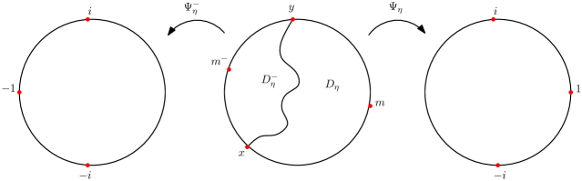
Figure 4.1: An illustration of the domains and maps used in Theorem 4.1.

Theorem 4.1.

Suppose $\kappa\in(0,4]$ and $\eta$ is a chordal SLE_κ from $x$ to $y$ in $\partial\mathbf{D}$. Define the domains $D_{\eta}$ and $D_{\eta}^{-}$ and the event $\mathcal{E}_{\epsilon}^{s;u}(\eta,z,;c)$ as above; and with $\alpha(s)$ and $\alpha_{0}(s)$ as in (3.2), define

$$\gamma(s):=\alpha(s)-2s+1=\frac{(4+\kappa)^{2}s^{2}}{8\kappa(1+s)}-2s+1,\qquad\gamma_{0}(s):=2\alpha_{0}(s)+2=\frac{2(4+\kappa)^{2}s(2+s)}{8\kappa(1+s)^{2}}+2.$$ (4.1)

Also define the events $\mathcal{G}(\cdot,\mu)$ as in Definition 2.5. For each $d\in(0,1)$, $\mu\in\mathcal{M}$, $c>0$, and $z\in B_{d}(0)$,

$$\mathbf{P}\left(\mathcal{E}_{\epsilon}^{s;u}(\eta,z;c)\cap\mathcal{G}(\Psi_{\eta},\mu)\cap\mathcal{G}(\Psi_{\eta}^{-},\mu)\right)\preceq\epsilon^{\gamma(s)-\gamma_{0}(s)u}.$$ (4.2)

Furthermore, for each $d\in(0,1)$ there exists $\mu\in\mathcal{M}$ such that for each $c>0$ and $u>0$ we can find $\epsilon_{0}>0$ such that for each $\epsilon\in(0,\epsilon_{0}]$ and each $z\in B_{d}(0)$,

$$\mathbf{P}\left(\mathcal{E}_{\epsilon}^{s;u}(\eta,z;c)\cap\mathcal{G}(\Psi_{\eta},\mu)\cap\mathcal{G}(\Psi_{\eta}^{-},\mu)\right)\succeq\epsilon^{\gamma(s)+\gamma_{0}(s)u}.$$ (4.3)

In (4.2) and (4.3) the implicit constants are independent of $\epsilon$ and uniform for $z\in B_{d}(0)$ and for $|x-y|$ bounded below by a positive constant.

The proof of Theorem 4.1 proceeds as follows. First we use Theorem 3.1 and a change of variables to prove estimates for the area of the sets where certain finite-time analogs of the sets of Theorem 4.1 occur. This is done in Section 4.2. This subsection also contains a result which allows us to extend the estimate for deterministic times to estimates for certain stopping times, which will be needed in the sequel. Then, in Section 4.3, we prove several lemmas comparing finite time and infinite time maps and use these lemmas to obtain estimates for the area of the set of points where the events of Theorem 4.1 occur. Finally, we complete the proof of Theorem 4.1 in Section 4.4 by proving a lemma which gives that the probabilities of the events of Theorem 4.1 do not depend too strongly on $z$, so that pointwise estimates can be deduced from area estimates. In Section 4.5 we deduce an analog of Theorem 4.1 for the curve stopped at a finite time.

4.2 Area estimates and stopping estimates for finite time maps

In this section we will prove estimates for the expected area of the set of points where finite-time analogs of the events of Theorem 4.1 occur. We will also prove a result which allows us to compare probabilities for events at stopping times whose difference is bounded. Suppose we are in the setting of Theorem 4.1.

Definition 4.2.

Let $\eta$ be a chordal $\operatorname{SLE}_{\kappa}$ from $-i$ to $i$ in $\mathbf{D}$. Define its forward centered Loewner maps $(f_{t})$ as in Section 3.5. For $t,\epsilon,u,\delta,c>0$, $s\in(-1,1)$, and $z\in\mathbf{D}$, let $E_{\epsilon}^{s;u}(\eta,z;t,\delta,c)$ be the event that the following hold.

1. $c^{-1}\epsilon^{s+u}\leq|f_{t}^{\prime}(z)|\leq c\epsilon^{s-u}$.

2. $c^{-1}\epsilon^{1-s+u}\leq\operatorname{dist}(z,\eta^{t})\leq c\epsilon^{1-s-u}$.

3. $|f_{t}(z)-i|$ and $|f_{t}(z)+i|$ are both at least $\delta$.

Let $A_{\epsilon}^{s;u}(\eta;t,\delta,c)$ be the set of $z\in\mathbf{D}$ for which $E_{\epsilon}^{s;u}(\eta,z;t,\delta,c)$ occurs.

Lemma 4.3.

Suppose we are in the setting of Theorem 4.1 with $x=-i$ and $y=i$. Fix $\delta>0$. Define the sets $A_{\epsilon}^{s;u}(\eta;t,\delta,c)$ as in Definition 4.2 and the events $\mathcal{G}(f_{t},\mu)$ as in Definition 2.5. For any choice of parameters $t,c,\mu$ and any $d\in(0,1)$,

$$\mathbf{E}\left[\operatorname{Area}(A_{\epsilon}^{s,u}(\eta;t,\delta,c)\cap B_{d}(0))\mathbf{1}_{\mathcal{G}(f_{t},\mu)}\right]\preceq\epsilon^{\gamma(s)-\gamma_{0}(s)u}$$ (4.4)

with the implicit constants independent of $\epsilon$ and uniform for $z\in B_{d}(0)$. Moreover, there exists $t_{*}>0$ such that for each $t\geq t_{*}$, there exists $\mu\in\mathcal{M}$ and $d\in(0,1)$ such that for each $c>0$ and each $u>0$, there exists $\epsilon_{0}>0$ such that for $\epsilon\in(0,\epsilon_{0}]$,

$$\mathbf{E}\left[\operatorname{Area}(A_{\epsilon}^{s;u}(\eta;t,\delta,c)\cap B_{d}(0))\mathbf{1}_{\mathcal{G}(f_{t},\mu)}\right]\succeq\epsilon^{\gamma(s)+\gamma_{0}(s)u},$$ (4.5)

with the implicit constants independent of $\epsilon$ and uniform for $z\in B_{d}(0)$.

Proof.

This will follow by integrating the estimate of Corollary 3.11 and performing a change of variables. Let $\underline{A}_{\epsilon}^{s;u}=\underline{A}_{\epsilon}^{s;u}(\eta;t,\delta,c,d)$ be the set of $z\in\mathbf{D}$ such that

1. $c^{-1}\epsilon^{1+u}\leq 1-|z|\leq c\epsilon^{1-u}$;

2. $|z-i|$ and $|z+i|$ are each at least $\delta$;

3. The event $\underline{E}_{\mathbf{D}}^{s;u}(z;t,c,d)$ of Section 3.5 occurs.

By (3.26) in Corollary 3.11, if the first two conditions in the definition of $\underline{A}_{\epsilon}^{s;u}$ hold for some $z\in\mathbf{D}$, then

$$\mathbf{P}\left(\underline{E}_{\mathbf{D}}^{s;u}(z;t,c,d)\cap\mathcal{G}(f_{t},\mu)\right)\preceq\epsilon^{\alpha(s)-\alpha_{0}(s)u}.$$

By integrating this over all such $z$, we get

$$\mathbf{E}\left[\operatorname{Area}(\underline{A}_{\epsilon}^{s;u})\mathbf{1}_{G(f_{t},\mu)}\right]\preceq\epsilon^{\alpha(s)+1-(\alpha_{0}(s)+1)u}.$$ (4.6)

Similarly, suppose $t$, $d$, $\mu$, and $\epsilon_{0}$ are chosen so that (3.27) in Corollary 3.11 holds. Then for $\epsilon\in(0,\epsilon_{0}]$,

$$\mathbf{E}\left[\operatorname{Area}(\underline{A}_{\epsilon}^{s;u})\mathbf{1}_{G(f_{t},\mu)}\right]\succeq\epsilon^{\alpha(s)+1+(\alpha_{0}(s)+1)u}.$$ (4.7)

By the change of variables formula,

$$\operatorname{Area}\left(A_{\epsilon}^{s;u}(\eta;t,\delta,c)\cap B_{d}(0)\right)=\int_{f_{t}(A_{\epsilon}^{s;u}(\eta;t,\delta,c)\cap B_{d}(0))}|(f_{t}^{-1})^{\prime}(z)|^{2}\,dz.$$ (4.8)

The Koebe quarter theorem implies

$$\underline{A}_{\epsilon}^{s;u/2}(\eta;t,\delta,c^{\prime},d)\subset f_{t}\left(A_{\epsilon}^{s;u}(\eta;t,\delta,c)\cap B_{d}(0)\right)\subset\underline{A}_{\epsilon}^{s;2u}(\eta;t,\delta,c^{\prime\prime},d)$$

for appropriate $c^{\prime},c^{\prime\prime}>0$, depending only on $c$. Thus (4.6) implies (4.4). Similarly (4.7) implies (4.5). ∎

In the remainder of this subsection we record a straightforward estimate which allows us to transfer estimates between stopping times and deterministic times.

Lemma 4.4.

Let $\eta$ be a chordal $\operatorname{SLE}_{\kappa}$ from $-i$ to $i$ in $\mathbf{D}$ with centered Loewner maps $(f_{t})$. Let $\tau,\tau^{\prime}$ be stopping times for $\eta$ and suppose there is a deterministic time $T>0$ such that a.s. $\tau\leq\tau^{\prime}\leq T$. For any $c>0$, $\mu\in\mathcal{M}$, and $\delta>0$, we can find $c^{\prime}>0$, $\delta^{\prime}>0$, and $\mu^{\prime}\in\mathcal{M}$ such that for each $u>0$, there is an $\epsilon_{0}=\epsilon_{0}(u,c,\mu,\delta)>0$ such that for each $z\in\mathbf{D}$ and each $\epsilon\in(0,\epsilon_{0}]$,

$$\mathbf{P}\left(E_{\epsilon}^{s;u}(\eta,z;\tau,\delta,c)\cap\mathcal{G}(f_{\tau},\mu)\right)\preceq\mathbf{P}\left(E_{\epsilon}^{s;u}(\eta,z;\tau^{\prime},\delta^{\prime},c^{\prime})\cap G(f_{\tau^{\prime}},\mu^{\prime})\right),$$ (4.9)

with the implicit constant uniform for $z$ in compact subsets of $\mathbf{D}$ and independent of $\epsilon$.

Proof.

Let $H$ be the event that the SLE_κ curve $f_{\tau}(\eta\setminus\eta^{\tau})$ stays in the tube $\{z\in\mathbf{D}:-\delta/100\leq\operatorname{Re}z\leq\delta/100\}$ until time $T$. By Lemma 2.17 and the strong Markov property, $\mathbf{P}(H\,|\,\eta^{\tau})\succeq 1$, with deterministic implicit constant depending only on $\delta$. On the other hand, if $\epsilon$ is sufficiently small relative to $\delta$ (so that $f_{\tau}(z)$ is within distance $\delta/100$ of $\partial\mathbf{D}$ on $E_{\epsilon}^{s;u}(\eta,z;\tau,\delta,c)\cap\mathcal{G}(f_{\tau},\mu)$, say) then $f_{\tau}(z)$ lies at distance at least $\delta/2$ from this tube on the event $E_{\epsilon}^{s;u}(\eta,z;\tau,\delta,c)\cap\mathcal{G}(f_{\tau},\mu)$. Since $\tau^{\prime}-\tau\leq T$, it follows easily that

$$E_{\epsilon}^{s;u}(\eta,z;\tau,\delta,c)\cap\mathcal{G}(f_{\tau},\mu)\cap H\subset E_{\epsilon}^{s;u}(\eta,z;\tau^{\prime},\delta^{\prime},c^{\prime})\cap G(f_{\tau^{\prime}},\mu^{\prime})$$

for appropriate $c^{\prime}$, $\delta^{\prime}$, and $\mu^{\prime}$ as in the statement of the lemma. Thus

$$\mathbf{P}\left(E_{\epsilon}^{s;u}(\eta,z;\tau^{\prime},\delta^{\prime},c^{\prime})\cap G(f_{\tau^{\prime}},\mu^{\prime})\,|\,E_{\epsilon}^{s;u}(\eta,z;\tau,\delta,c)\cap\mathcal{G}(f_{\tau},\mu)\right)\succeq 1,$$

so (4.9) holds. ∎

4.3 Comparison lemmas

In this subsection we prove several lemmas comparing probabilities of sets associated with the finite time Loewner maps to probabilities of sets associated with the infinite time Loewner maps of Theorem 4.1, and use these results to estimate the area of the set where the event of Theorem 4.1 occurs.

The next lemma is needed for the proof of the lower bound in Theorem 4.1.

Lemma 4.5.

Suppose we are in the setting of Theorem 4.1 with $x=-i$ and $y=i$. Fix $d\in(0,1)$. For each $\delta>0$, $\mu\in\mathcal{M}$, and $c>0$, there exists $\mu^{\prime}\in\mathcal{M}$ and $c^{\prime}>0$ such that for each $u>0$, there exists $\epsilon_{0}=\epsilon_{0}(c,c^{\prime},u,\delta,\mu,\mu^{\prime},d)>0$ such that for $z\in B_{d}(0)$ and $\epsilon\in(0,\epsilon_{0}]$,

$$\mathbf{P}\left(\mathcal{E}_{\epsilon}^{s;u}(\eta,z;c^{\prime})\cap\mathcal{G}(\Psi_{\eta},\mu^{\prime})\cap\mathcal{G}(\Psi_{\eta}^{-},\mu^{\prime})\right)\succeq\mathbf{P}\left(E_{\epsilon}^{s;u}(\eta,z;t,\delta,c)\cap\{\operatorname{Re}f_{t}(z)\geq 0\}\cap\mathcal{G}(f_{t},\mu)\right),$$ (4.10)

with implicit constants independent of $\epsilon$ and uniform for $z\in B_{d}(0)$.

Proof.

The idea of the proof is that if we condition on the event on the right side of (4.10), then with uniformly positive conditional probability the curve $\eta|_{[t,\infty)}$ will behave nicely and hence the event on the left in (4.10) will also occur (this is similar to the idea of the proof of Lemma 4.4, but slightly more involved since we have to go all the way to time $\infty$).

To explain this formally, let $f_{t}:\mathbf{D}\setminus\eta^{t}\rightarrow\mathbf{D}$ be the centered forward Loewner maps for $\eta$ as in Section 4.2. For $t\geq 0$, let $\eta_{t}=f_{t}(\eta|_{[t,\infty)})$. Also let $D_{t}$ be the connected component of $\mathbf{D}\setminus\eta_{t}$ containing 1 on its boundary and let $D_{t}^{-}$ be the other connected component of $\mathbf{D}\setminus\eta_{t}$. Let $\Psi_{t}:D_{t}\rightarrow\mathbf{D}$ (resp. $\Psi_{t}^{-}:D_{t}\rightarrow\mathbf{D}$) be the unique conformal maps fixing $-i,i,1$ (resp. $-i,i,-1$). Let $b_{t}$ (resp. $b_{t}^{-}$) be the image of the right (resp. left) side of $-i$ under $f_{t}$. Finally, let $\psi_{t}$ (resp. $\psi_{t}^{-}$) be the conformal automorphism of $\mathbf{D}$ fixing $i$, taking $\Psi_{t}(b_{t})$ to $-i$, and taking $\Psi_{t}(f_{t}(1))$ to $1$ (resp. fixing $i$, taking $\Psi_{t}^{-}(b_{t}^{-})$ to $-i$, and taking $\Psi_{t}^{-}(f_{t}(-1))$ to -1). Then for each $t$,

$$\Psi_{\eta}=\psi_{t}\circ\Psi_{t}\circ f_{t},\qquad\Psi_{\eta}^{-}=\psi_{t}^{-}\circ\Psi_{t}^{-}\circ f_{t}.$$ (4.11)

Moreover, $(\Psi_{t},\Psi_{t}^{-})$ and $f_{t}$ are independent and $\Psi_{t}\overset{d}{=}\Psi_{\eta}$, $\Psi_{t}^{-}\overset{d}{=}\Psi_{\eta}^{-}$. See Figure 4.2 for an illustration of some of these maps.

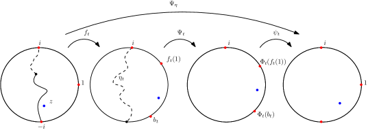
Figure 4.2: An illustration of the maps used in the proof of Lemma 4.5 for the right side of $\mathbf{D}$. The red points are the images of $-i,i$, and $1$ under the various maps. The last map $\psi_{t}$ takes these points back to their original positions so that by composing all three maps we recover the original map $\Psi_{\eta}$.

For $C>1$, $\mu^{\prime}\in\mathcal{M}$, and $w\in\mathbf{D}$, let $F(w)=F(w;t,C,\mu^{\prime})$ be the event that $w\in D_{t}$, $C^{-1}\leq|\Psi_{t}^{\prime}(w)|\leq C$, $\operatorname{dist}(w,\eta_{t})=\operatorname{dist}(w,\partial\mathbf{D})$, and $\mathcal{G}(\Psi_{t},\mu^{\prime})\cap\mathcal{G}(\Psi_{t}^{-},\mu^{\prime})$ occurs. By Lemma 2.17, for each $\delta>0$, we can find $C>1$ and $\mu^{\prime}\in\mathcal{M}$ such that for each $w\in\mathbf{D}$ lying at distance at least $\delta$ from $\pm i$ with $\operatorname{Re}w\geq 0$, we have that $\mathbf{P}(F(w))\succeq 1$, with the implicit constant independent of $\epsilon$ and uniform for $w$ satisfying the conditions above.

If we let

$$F^{*}(z):=E_{\epsilon}^{s;u}(\eta,z;t,\delta,c)\cap\{\operatorname{Re}f_{t}(z)\geq 0\}\cap\mathcal{G}(f_{t},\mu)\cap F(f_{t}(z)),$$

then by independence of $f_{t}$ and $\eta_{t}$ and our choice of parameters for $F(\cdot)$,

$$\mathbf{P}\left(F^{*}(z)\right)\asymp\mathbf{P}\left(E_{\epsilon}^{s;u}(\eta,z;t,\delta,c)\cap\{\operatorname{Re}f_{t}(z)\geq 0\}\cap\mathcal{G}(f_{t},\mu)\right).$$ (4.12)

By the “$\mathcal{G}$” condition in the definition of $F(f_{t}(z))$, we have that $|\psi_{t}^{\prime}|$ and $|(\psi_{t}^{-})^{\prime}|$ are bounded above and below by positive $\epsilon$-independent constants on the event $F^{*}(z)$. Hence it follows from (4.11) that $F^{*}(z)\subset\mathcal{E}_{\epsilon}^{s;u}(\eta,z;c^{\prime})\cap\mathcal{G}(\Psi_{\eta},\mu^{\prime\prime})\cap\mathcal{G}(\Psi_{\eta}^{-},\mu^{\prime\prime})$ for some $c^{\prime}>0$ and some $\mu^{\prime\prime}\in\mathcal{M}$ which do not depend on $\epsilon$ and are uniform for $z\in B_{d}(0)$. By combining this with (4.12) we get (4.10) (with $\mu^{\prime\prime}$ in place of $\mu^{\prime}$). ∎

Our next lemma is needed for the proof of the upper bound in Theorem 4.1. The proof in this case is much more involved than the proof of Lemma 4.5. Intuitively, the reason for this is that it is easy to construct a full SLE curve which contains a given segment of an SLE curve run up to finite time (just grow the rest of the curve) but harder to construct an SLE run up to a finite time which has nice behavior and contains a conformal image of a given full SLE curve (one has to use reversibility and define appropriate regularity conditions for an SLE and its time reversal in order to successfully “splice in” the given full SLE curve).

Lemma 4.6.

Suppose we are in the setting of Theorem 4.1 with $x=-i$ and $y=i$. Fix $d\in(0,1)$. There is a $\delta>0$ such that for each $\mu\in\mathcal{M}$ and $c>0$, there exists $\mu^{\prime}\in\mathcal{M}$ and $c^{\prime}>0$ such that for each $u>0$, there exists $\epsilon_{0}>0$ and a bounded stopping time $\tau$ for $\eta$ such that for each $z\in B_{d}(0)$ and each $\epsilon\in(0,\epsilon_{0}]$,

$$\mathbf{P}\left(\mathcal{E}^{s;u}(\eta,z;c)\cap\mathcal{G}(\Psi_{\eta},\mu)\cap\mathcal{G}(\Psi_{\eta}^{-},\mu)\right)\preceq\mathbf{P}\left(E_{\epsilon}^{s;u}(z;\tau,\delta,c^{\prime})\cap\mathcal{G}(f_{\tau},\mu^{\prime})\right)$$ (4.13)

with the implicit constants independent of $\epsilon$ and uniform for $z\in B_{d}(0)$.

Proof.

Suppose $\mathcal{E}^{s;u}(\eta,z;c)\cap\mathcal{G}(\Psi_{\eta},\mu)\cap\mathcal{G}(\Psi_{\eta}^{-},\mu)$ occurs. We will prove the lemma by growing some more of the curve out from $-i$ and $i$ to get a new curve $\widetilde{\eta}\overset{d}{=}\eta$ with the property that $E_{\epsilon}^{s;u}(\widetilde{\eta},z;\tau,\delta,c^{\prime})\cap\mathcal{G}(f_{\tau},\mu^{\prime})$ occurs for an appropriate bounded stopping time $\tau$ and the derivatives of the conformal maps associated with $\widetilde{\eta}^{\tau}$ and with $\eta$ at $z$ are comparable.

To this end, let $\eta_{0}$ be a chordal $\operatorname{SLE}_{\kappa}$ from $-i$ to $i$ in $\mathbf{D}$, independent of $\eta$. Let $\overline{\eta}_{0}$ be its time reversal. Then $\overline{\eta}_{0}$ has the law of a chordal $\operatorname{SLE}_{\kappa}$ from $i$ to $-i$ [Zha08b]. Fix parameters $\delta_{0},C,\beta,\zeta,r,a>0$, and $\mu_{0}\in\mathcal{M}$ and suppose $\zeta\ll 1-d$. Let $P$ be the event that the following is true.

1. Let $\overline{T}$ be the first time $\overline{\eta}_{0}$ gets within distance $e^{-\beta}$ of $z$. Then $\overline{T}<\infty$ and $\overline{\eta}_{0}^{\overline{T}}$ is disjoint from $(\mathbf{D}\setminus\mathbf{H})\cup B_{1/2}(1)$.

2. For each $t\geq 0$, let $\phi_{t}:\mathbf{D}\setminus(\eta_{0}^{t}\cup\overline{\eta}_{0}^{\overline{T}})$ be the unique conformal map fixing $z$ and taking $\overline{\eta}_{0}(\overline{T})$ to $i$. Let $T$ be the first time $t$ that $\phi_{t}(\eta_{0}(t))=-i$ and $|\eta_{0}(t)-z|\leq 2e^{-\beta}$. Then $T<\infty$ and $\eta_{0}^{T}$ is disjoint from $(\mathbf{D}\cap\mathbf{H})\cup B_{1/2}(1)$.

3. Henceforth put $\phi=\phi_{T}$. We have $C^{-1}\leq|(\phi^{-1})^{\prime}(w)|\leq C$ for each $w\in B_{(1+d)/2}(0)$.

4. We have $\phi^{-1}\left(B_{\delta_{0}}(-i)\cup B_{\delta_{0}}(i)\cup B_{1-r}(0)\right)\subset B_{(1-d)/2}(z)$.

5. Let $\overline{\sigma}$ be the last exit time of $\overline{\eta}_{0}$ from $B_{\zeta}(i)$ before time $\overline{T}$. Then $\overline{\eta}_{0}^{\overline{\sigma}}\subset B_{2\zeta}(i)$.

6. Let

   $$K:=\eta_{0}^{T}\cup\overline{\eta}_{0}([\overline{\sigma},\overline{T}])\cup B_{(1-d)/2}(z).$$ (4.14)

   The harmonic measure from $i$ of each side of $K\cap B_{(1-d)/2}(i)$ and each side of $K\cap B_{(1-d)/2}(-i)$ in the Schwarz reflection of $\mathbf{D}\setminus K$ across $[-1,1]_{\partial\mathbf{D}}$ is at least $a$.

7. $\mathcal{G}^{\prime}(K,\mu_{0})$ occurs (Definition 2.6).

See Figure 4.3 for an illustration of the event $P$. In what follows, all implicit constants are required to depend only on $\mu$, $d$, and the parameters for $P$.

First we will argue that for any choice of the parameters $d,\zeta$, and $r$, we can choose the other parameters for $P$ in such a way that $\mathbf{P}(P)\succeq 1$. It follows from Lemma 2.17 and reversibility of SLE that conditions 1, 2, and 5 hold with positive probability depending only on $\beta$, $\zeta$, and $d$. By the Koebe growth theorem, if $\beta$ is chosen sufficiently large (depending on $r$ and $d$) and $\delta_{0}$ is chosen sufficiently small (depending only on $d$) then condition 4 also holds simultaneously with positive probability depending only on $\beta,\zeta,d$, $\delta_{0}$, and $r$. By choosing $C$ sufficiently large and $a$ and $\mu_{0}$ sufficiently small (see Lemma 2.7), depending only on $d$ and the other parameters for $P$, we can arrange that the remaining conditions in the definition of $P$ hold with probability arbitrarily close to 1. Thus $\mathbf{P}(P)\succeq 1$.

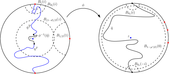
Figure 4.3: An illustration of the event $P$ and the curve $\widetilde{\eta}$ used in the proof of Lemma 4.6. The red points are $-i$, $i$, and 1 and their images under $\phi$.

Let $\widetilde{\eta}=\eta_{0}$ on the event that $P$ does not occur. On $P$, let $\widetilde{\eta}=\phi^{-1}(\eta)\cup\eta_{0}^{T}\cup\overline{\eta}^{\overline{T}}$, parameterized in such a way that its image under the conformal map from $\mathbf{D}$ to $\mathbf{H}$ taking $-i$ to $0$, $i$ to $\infty$, and $0$ to $i$ is parameterized by capacity. By the Markov property and reversibility of SLE, $\widetilde{\eta}$ has the same law as $\eta$. Let $(\widetilde{f}_{t})$ be the centered Loewner maps for $\widetilde{\eta}$. Let

$$\widetilde{\mathcal{E}}=\mathcal{E}^{s;u}_{\epsilon}(\eta,z;c)\cap\mathcal{G}(\Psi_{\eta},\mu)\cap\mathcal{G}(\Psi_{\eta}^{-},\mu)\cap P.$$

Let $\tau$ be the hitting time of $B_{\zeta}(i)$ by $\widetilde{\eta}$. Then $\tau$ is a bounded stopping time for $\widetilde{\eta}$. Furthermore, if we choose $\zeta$ sufficiently small relative to $d$ (independently of $\epsilon$) then on the event $\widetilde{\mathcal{E}}$ we have $\widetilde{\eta}\setminus\widetilde{\eta}^{\tau}=\overline{\eta}_{0}^{\overline{\sigma}}$, with $\overline{\sigma}$ as in condition 5 in the definition of $P$.

We claim that if the parameters for $P$ are chosen appropriately (independently of $\epsilon$ and $z\in B_{d}(0)$) then for sufficiently small $\epsilon>0$,

$$\widetilde{\mathcal{E}}\subset E_{\epsilon}^{s;u}(\widetilde{\eta},z;\tau,\delta,\widetilde{c})\cap\mathcal{G}(\widetilde{f}_{\tau},\widetilde{\mu})$$ (4.15)

for some $\widetilde{\mu}\in\mathcal{M}$ depending only on $d$ and some $\widetilde{c}>0$ and $\widetilde{\mu}\in\mathcal{M}$, depending only on $d$, $\mu$, $c$, and the parameters for $P$. Given the claim (4.15), our desired result (4.13) follows by taking probabilities and noting that $P$ is independent from $\eta$.

By condition 4 in the definition of $P$, on the event $\widetilde{\mathcal{E}}$ we have $\widetilde{\eta}^{\tau}\subset K$, as in (4.14), provided $r$ is chosen sufficiently small, depending only on $\mu$ and $\delta_{0}$. By condition 7 in the definition of $P$ and Lemma 2.8, we can find $\widetilde{\mu}\in\mathcal{M}$ depending only on $\mu$, $d$ and the parameters for $P$ such that $\widetilde{\mathcal{E}}\subset\mathcal{G}(\widetilde{f}_{\tau},\widetilde{\mu})$. By condition 4.14 in the definition of $P$, we can find $\delta>0$ depending only on $a$ such that $\widetilde{f}_{\tau}(z)$ lies at distance at least $\delta$ from $\pm i$ on $\widetilde{\mathcal{E}}$. That is, condition 3 in the definition of $E_{\epsilon}^{s;u}(\widetilde{\eta},z;\tau,\delta,\widetilde{c})$ holds on $\widetilde{\mathcal{E}}$.

By condition 3 in the definition of $P$, we have $\operatorname{dist}(z,\widetilde{\eta})\asymp\operatorname{dist}(z,\eta)$ on $P$. It therefore follows that condition 1 in the definition of $E_{\epsilon}^{s;u}(\widetilde{\eta},z;\tau,\delta,\widetilde{c})$ holds on $\widetilde{\mathcal{E}}$ for some $\widetilde{c}\asymp 1$.

It remains to show that condition 1 in the definition of $E_{\epsilon}^{s;u}(\widetilde{\eta},z;\tau,\delta,\widetilde{c})$ holds on $\widetilde{\mathcal{E}}$ provided $\widetilde{c}\asymp 1$ is chosen sufficiently large. It is enough to show $|\widetilde{f}_{\tau}^{\prime}(z)|\asymp|\Psi_{\eta}^{\prime}(z)|$ on $\widetilde{\mathcal{E}}$. We will do this in two stages. Let $\Psi_{\widetilde{\eta}}$ be as in Section 4.1 with $\widetilde{\eta}$ in place of $\eta$. First we will show that $|\Psi_{\eta}^{\prime}(z)|\asymp|\Psi_{\widetilde{\eta}}^{\prime}(z)|$, and then we will show that $|\Psi_{\widetilde{\eta}}^{\prime}(z)|\asymp|\widetilde{f}_{\tau}^{\prime}(z)|$.

For the first stage, let $g$ be the conformal automorphism of $\mathbf{D}$ taking $\Psi_{\eta}(\phi(-i^{+}))$ to $-i$, $\Psi_{\eta}(\phi(i^{-}))$ to $i$, and $\Psi_{\eta}(\phi(1))$ to 1. Then

$$\Psi_{\widetilde{\eta}}=g\circ\Psi_{\eta}\circ\phi.$$ (4.16)

By condition 7 in the definition of $P$, together with the definition of $\widetilde{\mathcal{E}}$, $|g^{\prime}|\asymp 1$ uniformly on $\mathbf{D}$ on $\widetilde{\mathcal{E}}$, so by condition 3 in the definition of $P$, we have $|\Psi_{\widetilde{\eta}}^{\prime}(z)|\asymp|\Psi_{\eta}^{\prime}(z)|$ on $\widetilde{\mathcal{E}}$.

For the second stage, let $\Psi_{\widetilde{\eta}^{\tau}}$ be the conformal map from $\mathbf{D}\setminus\widetilde{\eta}^{\tau}$ to $\mathbf{D}$ taking $-i^{+}$ to $-i$ and fixing $i$ and 1. Then $\Psi_{\widetilde{\eta}^{\tau}}$ differs from $\widetilde{f}_{\tau}$ by a conformal automorphism of $\mathbf{D}$ taking $\widetilde{f}_{\tau}(-i^{+})$ to $-i$ and $\widetilde{f}_{\tau}(1)$ to 1. Since $\mathcal{G}(\widetilde{f}_{\tau},\widetilde{\mu})$ holds on $\widetilde{\mathcal{E}}$,

$$|\Psi_{\widetilde{\eta}^{\tau}}^{\prime}(z)|\asymp|\widetilde{f}_{\tau}^{\prime}(z)|.$$ (4.17)

Let $I$ be the arc of $\partial\mathbf{D}$ of length $\zeta$ centered at 1. By condition 7 in the definition of $P$ (c.f. Remark B.2), the lengths of $\Psi_{\widetilde{\eta}}(I)$ and $\Psi_{\widetilde{\eta}^{\tau}}(I)$ are $\succeq 1$ on $\widetilde{\mathcal{E}}$. By conditions 1, 4, and 5 in the definition of $P$ and a study of the harmonic measure from $1$ in the Schwarz reflection of $D_{\widetilde{\eta}}$, the distances from $\Psi_{\widetilde{\eta}}(z)$ to $\Psi_{\widetilde{\eta}}(I)$ and from $\Psi_{\widetilde{\eta}^{\tau}}(z)$ to $\Psi_{\widetilde{\eta}^{\tau}}(I)$ are $\succeq 1$ on $\widetilde{\mathcal{E}}$ provided $\zeta$ is chosen sufficiently small relative to $d$. By Lemma B.1, it holds on $\widetilde{\mathcal{E}}$ that

$$|\Psi_{\widetilde{\eta}}^{\prime}(z)|\asymp\frac{\operatorname{hm}^{z}(I;D_{\widetilde{\eta}})}{\operatorname{dist}(z,\widetilde{\eta})}\quad\operatorname{and}\quad|\Psi_{\widetilde{\eta}^{\tau}}^{\prime}(z)|\asymp\frac{\operatorname{hm}^{z}(I;\mathbf{D}\setminus\widetilde{\eta}^{\tau})}{\operatorname{dist}(z,\widetilde{\eta}^{\tau})}.$$ (4.18)

By the conformal invariance of harmonic measure, $\operatorname{hm}^{z}(I;D_{\widetilde{\eta}})$ is the same as the probability that a Brownian motion started from $\Psi_{\widetilde{\eta}^{\tau}}(z)$ exits $\mathbf{D}$ in $\Psi_{\widetilde{\eta}^{\tau}}(I)$ before hitting $\Psi_{\widetilde{\eta}^{\tau}}(\widetilde{\eta}([\tau,\infty))$. By conditions 5 and 4.14 in the definition of $P$, if $\zeta$ is chosen sufficiently small, independently of $\epsilon$, then on $\widetilde{\mathcal{E}}$, the distance from $\Psi_{\widetilde{\eta}^{\tau}}(\widetilde{\eta}([\tau,\infty))$ to $\Psi_{\widetilde{\eta}^{\tau}}(z)\cup\Psi_{\widetilde{\eta}^{\tau}}(I)$ is at least a deterministic $\epsilon$-independent constant; and the diameter of $\Psi_{\widetilde{\eta}^{\tau}}(\widetilde{\eta}([\tau,\infty))$ is smaller than $1/100$ times this constant (here we again use harmonic measure from 1). Therefore, the probability that a Brownian motion started from $\Psi_{\widetilde{\eta}^{\tau}}(z)$ exits $\mathbf{D}$ in $\Psi_{\widetilde{\eta}^{\tau}}(I)$ before hitting $\Psi_{\widetilde{\eta}^{\tau}}(\widetilde{\eta}([\tau,\infty))$ is proportional to the probability that a Brownian motion started from $\Psi_{\widetilde{\eta}^{\tau}}(z)$ exits $\mathbf{D}$ in $\Psi_{\widetilde{\eta}^{\tau}}(I)$. That is, $\operatorname{hm}^{z}(I;D_{\widetilde{\eta}})\asymp\operatorname{hm}^{z}(I;\mathbf{D}\setminus\widetilde{\eta}^{\tau})$ on $\widetilde{\mathcal{E}}$. By combining this with (4.17) and (4.18), we conclude. ∎

Now we can transfer our area estimates for the finite time sets to area estimates for the time infinity sets.

Lemma 4.7.

Suppose we are in the setting of Theorem 4.1 with $x=-i$ and $y=i$. Let $\mathcal{A}_{\epsilon}^{s;u}(\eta,c)$ be the set of $z\in\mathbf{D}$ for which $\mathcal{E}_{\epsilon}^{s;u}(\eta,z;c)$ occurs. For each $d\in(0,1)$, each $\mu\in\mathcal{M}$, and each $c>0$,

$$\mathbf{E}\left(\operatorname{Area}(\mathcal{A}_{\epsilon}^{s;u}(\eta;c)\cap B_{d}(0))\mathbf{1}_{\mathcal{G}(\Psi_{\eta},\mu)\cap\mathcal{G}(\Psi_{\eta}^{-},\mu)}\right)\preceq\epsilon^{\gamma(s)-\gamma_{0}(s)u}.$$ (4.19)

Furthermore, there exists $d\in(0,1)$ such that for each $c>0$, there exists $\mu\in\mathcal{M}$ and $\epsilon_{0}>0$ such that for each $\epsilon\in(0,\epsilon_{0}]$,

$$\mathbf{E}\left(\operatorname{Area}(\mathcal{A}_{\epsilon}^{s;u}(\eta;c)\cap B_{d}(0))\mathbf{1}_{\mathcal{G}(\Psi_{\eta},\mu)\cap\mathcal{G}(\Psi_{\eta}^{-},\mu)}\right)\succeq\epsilon^{\gamma(s)+\gamma_{0}(s)u}.$$ (4.20)

In both (4.19) and (4.20) the implicit constants depend on the other parameters but not on $\epsilon$.

Proof.

The relation (4.19) follows by integrating the estimate from Lemma 4.6 over $B_{d}(0)$, applying Lemma 4.4 to replace the stopping time $\tau$ with a deterministic time, then applying (4.4) from Lemma 4.3. The relation 4.20 similarly follows from Lemma 4.5. ∎

4.4 Proof of Theorem 4.1

To deduce Theorem 4.1 from the area estimate of Lemma 4.7, we need to argue that the probabilities of the events of Theorem 4.1 do not depend too strongly on $z$. This is accomplished in the next lemma.

Lemma 4.8.

Suppose we are in the setting of Theorem 4.1 with $x=-i$, $y=i$. Fix $d\in(0,1)$. For any $\mu\in\mathcal{M}$ and $c>0$, we can find $\mu^{\prime}\in\mathcal{M}$ and $c^{\prime}>0$ such that for each $z,w\in B_{d}(0)$ and $\epsilon\in(0,1)$,

$$\mathbf{P}\left(\mathcal{E}_{\epsilon}^{s;u}(\eta,w;c)\cap\mathcal{G}(\Psi_{\eta},\mu)\cap\mathcal{G}(\Psi_{\eta}^{-},\mu)\right)\preceq\mathbf{P}\left(\mathcal{E}_{\epsilon}^{s;u}(\eta,z;c^{\prime})\cap\mathcal{G}(\Psi_{\eta},\mu^{\prime})\cap\mathcal{G}(\Psi_{\eta}^{-},\mu^{\prime})\right)$$ (4.21)

with implicit constants independent of $\epsilon$ and uniform in $B_{d}(0)$.

Proof.

The basic idea of the proof is as follows. First we apply a conformal map taking $z$ to $w$ and fixing $-i$. The image of $\eta$ under such a map will be an $\operatorname{SLE}_{\kappa}$ with a new target point $b$. To compare such a curve to our original curve, we grow a carefully chosen segment of the new curve backward from $b$ in such a way that when we map back to $\mathbf{D}$, we get a chordal $\operatorname{SLE}_{\kappa}$ from $-i$ to $i$. We now commence with the details.

For $z,w\in B_{d}(0)$, let $\phi=\phi_{z,w}:\mathbf{D}\rightarrow\mathbf{D}$ be the unique conformal map fixing $-i$ and taking $z$ to $w$. Let $b:=\phi(i)$ and $\eta^{b}=\phi(\eta)$. The law of $\eta^{b}$ is that of a chordal $\operatorname{SLE}_{\kappa}$ process from $-i$ to $b$ in $\mathbf{D}$.

The map $\phi$ depends continuously on $z$ and $w$ in the topology of uniform convergence on compact subsets of $\mathbf{D}$. It follows that for any $\mu\in\mathcal{M}$ we can find a deterministic constant $c^{\prime}>0$ depending only on $c$, $\mu$, and $d$, linearly on $c$, and a deterministic $\mu^{\prime}\in\mathcal{M}$ depending only on $\mu$ and $d$ such that for $z,w\in B_{d}(0)$,

$$\mathcal{E}_{\epsilon}^{s;u}(\eta^{b},w;c)\cap\mathcal{G}(\Psi_{\eta^{b}},\mu)\cap\mathcal{G}(\Psi_{\eta^{b}}^{-},\mu)\subset\mathcal{E}_{\epsilon}^{s;u}(\eta,z;c^{\prime})\cap\mathcal{G}(\Psi_{\eta},\mu^{\prime})\cap\mathcal{G}(\Psi_{\eta^{b}}^{-},\mu^{\prime}).$$ (4.22)

Let $\overline{\eta}^{b}$ be the time reversal of $\eta^{b}$. Then $\overline{\eta}^{b}$ is a chordal $\operatorname{SLE}_{\kappa}$ from $b$ to $-i$ in $\mathbf{D}$ [Zha08b]. We give $\overline{\eta}^{b}$ the usual chordal parameterization, so that it is the conformal image of a chordal $\operatorname{SLE}_{\kappa}$ parameterized by capacity from $0$ to $\infty$ in $\mathbf{H}$. For each $t\geq 0$, let $\overline{g}_{t}:\mathbf{D}\setminus\overline{\eta}^{b}([0,t])\rightarrow\mathbf{D}$ be the unique conformal map fixing $-i$ and $w$. Let $\tau$ be the first time $t$ that $\overline{g}_{t}(\overline{\eta}^{b}(t))=i$.

Fix $\mu^{b}\in\mathcal{M}$ and let $\overline{E}^{b}$ be the event that $\tau$ is less than or equal to the first time $t$ that $\overline{\eta}^{b}$ hits $B_{d^{*}}(0)$, where

$$d^{*}:=1-\frac{1}{4}\inf_{z,w\in B_{d}(0)}\operatorname{dist}(\phi_{z,w}(B_{d}(0)),\partial\mathbf{D});$$

and the event $\mathcal{G}(\overline{g}_{\tau},\mu^{b})$ occurs. By Lemma 2.17, if $\mu^{b}$ is chosen sufficiently small then $\mathbf{P}(\overline{E}^{b})$ is a positive constant depending only on $\mu^{b}$ and $B_{d}(0)$.

By the Markov property, conditional on $\overline{E}^{b}$, the law of $\overline{g}_{\tau}(\overline{\eta}^{b}|_{[\tau,\infty)})$ is that of a chordal $\operatorname{SLE}_{\kappa}$ process from $i$ to $-i$ in $\mathbf{D}$. Therefore its time reversal $\widehat{\eta}:=\overline{g}_{\tau}^{b}(\eta|_{[0,\tau^{b}]})$, where $\tau^{b}$ is the time corresponding to $\tau$ under the time reversal, has the law of a chordal $\operatorname{SLE}_{\kappa}$ from $-i$ to $i$ in $\mathbf{D}$. In particular, $\widehat{\eta}\overset{d}{=}\eta$.

Define the open sets $D_{\eta^{b}},D_{\widehat{\eta}}$ and the maps $\Psi_{\eta^{b}},\Psi_{\widehat{\eta}}$ as in Section 4.1 with $\eta^{b},\widehat{\eta}$, resp., in place of $\eta$, except that in the definition of $\eta^{b}$ we use the points $\phi(-1)$ and $\phi(1)$ instead of the midpoints $m^{-}$ and $m$. Also let $\psi$ and $\psi^{-}$ be the conformal automorphisms of $\mathbf{D}$ such that

$$\Psi_{\eta^{b}}=\psi\circ\Psi_{\widehat{\eta}}\circ\overline{g}_{\tau}\quad\operatorname{and}\quad\Psi_{\eta^{b}}^{-}=\psi^{-}\circ\Psi_{\widehat{\eta}}^{-}\circ\overline{g}_{\tau}.$$

See Figure 4.4 for an illustration of some of these maps.

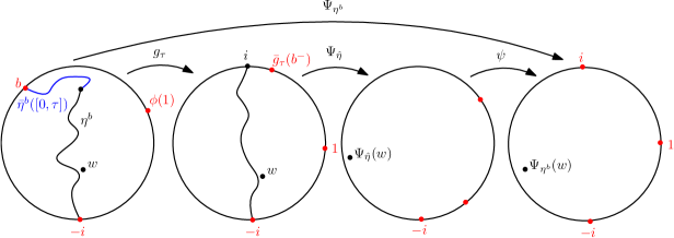
Figure 4.4: An illustration of the maps used in the proof of Lemma 4.8 on the event $\overline{E}^{b}$.

Since $\overline{E}^{b}\subset\mathcal{G}(\overline{g}_{\tau},\mu^{b})$, on the event $\overline{E}^{b}\cap\mathcal{E}_{\epsilon}^{s;u}(\widehat{\eta},w;c)\cap\mathcal{G}(\Psi_{\widehat{\eta}},\mu)\cap\mathcal{G}(\Psi_{\widehat{\eta}}^{-},\mu)$, it holds that $|\psi^{\prime}|$ and $|(\psi^{-})^{\prime}|$ are bounded above and below by deterministic positive constants depending only on $\mu^{b}$ and $\mu$. Furthermore, $\mathcal{G}(\psi,\mu_{2})\cap\mathcal{G}(\psi^{-},\mu_{2})$ holds for some $\mu_{2}\in\mathcal{M}$ depending on $\mu^{b},\mu$. The Koebe distortion theorem and the definition of $\overline{E}^{b}$ imply that $|g_{\tau}^{\prime}(w)|$ is bounded above and below by positive constants depending only on $d$ on the event $\overline{E}^{b}$. Hence for some $c_{0}>0$, independent of $\epsilon$ and uniform for $z,w\in B_{d}(0)$,

$$\overline{E}^{b}\cap\mathcal{E}_{\epsilon}^{s;u}(\widehat{\eta},w;c)\cap\mathcal{G}(\Psi_{\widehat{\eta}},\mu)\cap\mathcal{G}(\Psi_{\widehat{\eta}}^{-},\mu)\subset\mathcal{E}_{\epsilon}^{s;u}(\eta^{b},w;c_{0})\cap\mathcal{G}(\Psi_{\eta^{b}},\mu_{2}\circ\mu\circ\mu^{b})\cap\mathcal{G}(\Psi_{\eta^{b}}^{-},\mu_{2}\circ\mu\circ\mu^{b}).$$ (4.23)

By the Markov property and the fact that $\mathbf{P}(\overline{E}^{b})$ is uniformly positive,

$$\mathbf{P}\left(\overline{E}^{b}\cap\mathcal{E}_{\epsilon}^{s;u}(\widehat{\eta},w;c)\cap\mathcal{G}(\Psi_{\widehat{\eta}},\mu)\cap\mathcal{G}(\Psi_{\widehat{\eta}}^{-},\mu)\right)\asymp\mathbf{P}\left(\mathcal{E}_{\epsilon}^{s;u}(\widehat{\eta},w;c)\cap\mathcal{G}(\Psi_{\widehat{\eta}},\mu)\cap\mathcal{G}(\Psi_{\widehat{\eta}}^{-},\mu)\right).$$ (4.24)

Since $\widehat{\eta}\overset{d}{=}\eta$, (4.21) now follows from (4.22) (applied with $\mu_{2}\circ\mu\circ\mu^{b}$ in place of $\mu$, $c_{0}$ in place of $c$, and a possibly larger choice of $c^{\prime}$ and $\mu^{\prime}$), (4.23), and (4.24). ∎

Proof of Theorem 4.1.

By applying a coordinate change it is enough to consider the case $x=-i,$ $y=i$. By Lemma 4.8, for any $z\in B_{d}(0)$, we have, in the notation of that lemma,

$$\mathbf{P}\left(\mathcal{E}_{\epsilon}^{s;u}(\eta,z;c)\cap\mathcal{G}(\Psi_{\eta},\mu)\cap\mathcal{G}(\Psi_{\eta}^{-},\mu)\right)\preceq\mathbf{E}\left(\operatorname{Area}(\mathcal{A}_{\epsilon}^{s;u}(\eta,z;c^{\prime})\cap B_{d}(0))\mathbf{1}_{\mathcal{G}(\Psi_{\eta},\mu^{\prime})\cap\mathcal{G}(\Psi_{\eta}^{-},\mu^{\prime})}\right)$$

$$\mathbf{P}\left(\mathcal{E}_{\epsilon}^{s;u}(\eta,z;c^{\prime})\cap\mathcal{G}(\Psi_{\eta},\mu^{\prime})\cap\mathcal{G}(\Psi_{\eta}^{-},\mu^{\prime})\right)\succeq\mathbf{E}\left(\operatorname{Area}(\mathcal{A}_{\epsilon}^{s;u}(\eta,z;c)\cap B_{d}(0))\mathbf{1}_{\mathcal{G}(\Psi_{\eta},\mu)\cap\mathcal{G}(\Psi_{\eta}^{-},\mu)}\right),$$

where here $\mathcal{A}_{\epsilon}^{s;u}(\cdot)$ is the set where $\mathcal{E}_{\epsilon}^{s;u}(\cdot)$ occurs, as in Lemma 4.7. We conclude by combining this with Lemma 4.7 (and slightly decreasing $u$ and shrinking $\epsilon_{0}$ as in the proof of Lemma 4.7 to get a small enough constant in the event for lower bound). ∎

4.5 Finite time estimates

In this subsection we use Theorem 4.1 and the comparison lemmas of Section 4.3 to prove estimates for the finite time Loewner maps. The result of this subsection is not needed for the proof of our main result, and is stated only for the sake of completeness.

Theorem 4.9.

Let $\kappa\in(0,4]$. Let $(f_{t})$ be the centered Loewner maps of a chordal $\operatorname{SLE}_{\kappa}$ process $\eta$ from $-i$ to $i$ in $\mathbf{D}$. Fix $d\in(0,1)$. Define the events $E_{\epsilon}^{s;u}(z;t,\delta,c)$ as in Definition 4.2 and the sets $G(f_{t},\mu)$ as in Definition 2.5. For any $\mu\in\mathcal{M}$, $t,\delta,c>0$, $\epsilon>0$, and $z\in B_{d}(0)$,

$$\mathbf{P}\left(E_{\epsilon}^{s;u}(\eta,z;t,\delta,c)\cap\mathcal{G}(f_{t},\mu)\cap\{\operatorname{Re}f_{t}(z)\geq 0\}\right)\preceq\epsilon^{\gamma(s)-2\gamma_{0}(s)u}.$$ (4.25)

Moreover, there exists $t_{*}>0$, $\delta>0$, and $\mu\in\mathcal{M}$ such that for each $c>0$ and each $u>0$, there exists $\epsilon_{0}>0$ such that for $\epsilon\in(0,\epsilon_{0}]$ and $z\in B_{d}(0)$,

$$\mathbf{P}\left(E_{\epsilon}^{s;u}(\eta,z;t,\delta,c)\cap\mathcal{G}(f_{t},\mu)\right)\succeq\epsilon^{\gamma(s)+2\gamma_{0}(s)u}.$$ (4.26)

In (4.25) and (4.26) the implicit constants are independent of $\epsilon$ and uniform for $z\in B_{d}(0)$. The estimate (4.25) holds with $t$ replaced by a bounded stopping time. The estimate (4.26) holds with $t$ replaced by a bounded stopping time which is a.s. $\geq t_{*}$.

Proof.

The statement for deterministic times follows by combining Theorem 4.1 with Lemmas 4.4, 4.6 and 4.5. The statement for stopping times follows from this and Lemma 4.4. ∎

5 Upper bounds for multifractal and integral means spectra

In this section we will use the upper bounds in Theorems 3.1 and 4.1 to prove the Hausdorff dimension upper bounds in Theorem 1.1 as well the upper bound in Corollary 1.9.

5.1 Upper bound for the Hausdorff dimension of the subset of the circle

In this subsection we use Theorem 3.1 to obtain upper bounds on the Hausdorff dimension of the sets $\widetilde{\Theta}^{s}(\mathbf{D}\setminus K_{t})$ of Section 1.1 for the hulls $(K_{t})$ of a chordal $\operatorname{SLE}_{\kappa}$ from $-i$ to $i$ in $\mathbf{D}$. In light of Lemma 2.15, Proposition 5.1 implies the upper bounds for $\dim_{\mathcal{H}}\widetilde{\Theta}^{s;\geq}(D_{\eta})$ and $\dim_{\mathcal{H}}\widetilde{\Theta}^{s;\leq}(D_{\eta})$ in Theorem 1.1.

Proposition 5.1.

Let $\eta$ be a chordal $\operatorname{SLE}_{\kappa}$ process from $-i$ to $i$ in $\mathbf{D}$ with forward centered Loewner maps $(f_{t})$ (defined as in Section 3.5) and hulls $(K_{t})$. Let $\widetilde{\xi}(s)$, $s_{-}$, and $s_{+}$ be as in (1.3). For each $t>0$ and $s\in[-1,1]$, a.s.

$$\dim_{\mathcal{H}}\widetilde{\Theta}^{s;\geq}(\mathbf{D}\setminus K_{t})\leq\widetilde{\xi}(s),\qquad 0\leq s\leq s_{+}$$

$$\dim_{\mathcal{H}}\widetilde{\Theta}^{s;\leq}(\mathbf{D}\setminus K_{t})\leq\widetilde{\xi}(s),\qquad s_{-}\leq s\leq 0.$$ (5.1)

Almost surely, for each $s\notin[s_{-},s_{+}]$ we have $\widetilde{\Theta}^{s}(\mathbf{D}\setminus K_{t})=\emptyset$. In fact, for each $\delta>0$ and each $s>s_{+}$, it is a.s. the case that for small enough $\epsilon>0$,

$$|(f_{t}^{-1})^{\prime}((1-\epsilon)x)|\leq\epsilon^{-s},\quad\forall x\in\partial\mathbf{D}\>\text{with $|x-i|,|x+i|\geq\delta$ and $1-|f_{t}^{-1}(x)|\geq\delta$};$$ (5.2)

and similarly for $s<s_{-}$.

Remark 5.2.

If $\alpha(s)$ is as in (3.2) in the statement of Theorem 3.1, then $\widetilde{\xi}(s)=1-\alpha(s)$.

Proof of Proposition 5.1.

For $\delta>0$ and $s\in(-1,1)$, let

$$\widetilde{\Theta}^{s;*}_{\delta}(\mathbf{D}\setminus K_{t}):=\widetilde{\Theta}^{s;*}(\mathbf{D}\setminus K_{t})\cap\left\{x\in\partial\mathbf{D}:|x-i|,|x+i|\geq\delta,\quad 1-|f_{t}^{-1}(x)|\geq\delta\right\},$$

where $*$ stands for $\geq$ in the case $s\geq 0$ or $\leq$ in the case $s<0$. The reason for this definition is that it will allow us to apply the estimates of Proposition 3.6 after a change of coordinates from $\mathbf{D}$ to $\mathbf{H}$. By countable stability of Hausdorff dimension, to prove (5.1), it is enough to show that a.s.

$$\mathcal{H}^{\beta}(\widetilde{\Theta}^{s;*}_{\delta}(\mathbf{D}\setminus K_{t}))=0\quad\forall\>\delta>0,\quad\forall\>\beta>\widetilde{\xi}(s).$$

Henceforth fix $\delta$, $\beta$, and $s$ as above. Also let $s^{\prime}\in[0,s)$ (if $s\geq 0$) or $s^{\prime}\in(s,0)$ (if $s<0$) be chosen in such a way that $\widetilde{\xi}(s^{\prime})<\beta$.

For $n\in\mathbf{N}$ and $k\in\{1,\dots,2^{n}\}$, let

$$B_{n}^{k}:=\left\{w\in\mathbf{D}\,:\,\frac{\pi(k-1)}{2^{n-1}}\leq\operatorname{arg}w\leq\frac{\pi k}{2^{n-1}},\quad 2^{-n}\leq 1-|w|\leq 2^{-n+1}\right\}.$$ (5.3)

Let $E_{n}^{k}$ be the event there is a $w\in B_{n}^{k}$ with $1-|f_{t}^{-1}(w)|\geq\delta/2$ and

$$\begin{dcases}&|(f_{t}^{-1})^{\prime}(w)|\geq 2^{ns^{\prime}},\quad\text{if}\quad s\geq 0\\ &|(f_{t}^{-1})^{\prime}(w)|\leq 2^{ns^{\prime}},\quad\text{if}\quad s<0.\end{dcases}$$ (5.4)

Each $B_{n}^{k}$ can be covered by at most an $(n,k)$-independent constant number of balls of radius $<2^{-n-1}$, and each point of $B_{n}^{k}$ lies at distance at least $2^{-n}$ from $\partial\mathbf{D}$. So, the Koebe distortion and growth theorems imply that for sufficiently large $n$, on the event $E_{n}^{k}$ if $z$ is the center of one of these balls then $|(f_{t}^{-1})^{\prime}(z)|$ is at least (if $s\geq 0$) or at most (if $s<0$) an $(n,k)$-independent constant times $2^{ns^{\prime}}$ and $1-|f_{t}^{-1}(z)|\geq\delta/4$.

For $n\in\mathbf{N}$, let $\mathcal{K}_{n}$ be the set of those $k\in\{1,\dots,2^{n}\}$ such that $\exp(i\pi k/2^{n-1})$ lies at distance at least $\delta/2$ from $-i$ and $i$. By Proposition 3.6 and a change of coordinates to $\mathbf{H}$, whenever $k\in\mathcal{K}_{n}$,

$$\mathbf{P}(E_{n}^{k})\preceq 2^{-n(1-\widetilde{\xi}(s^{\prime}))}$$ (5.5)

where the implicit constant is independent of $n$ and uniform for $k\in\mathcal{K}_{n}$.

For $n\in\mathbf{N}$ and $k\in\{1,\dots,2^{n}\}$, let

$$I_{n}^{k}:=\left\{x\in\partial\mathbf{D}\,:\,\frac{\pi(k-1)}{2^{n-1}}\leq\operatorname{arg}x\leq\frac{\pi k}{2^{n-1}}\right\}.$$

For $m\in\mathbf{N}$, let $\mathcal{I}_{m}$ be the collection of those intervals $I_{n}^{k}$ for pairs $(n,k)$ such that $n\geq m$, $k\in\mathcal{K}_{n}$, and $E_{n}^{k}$ occurs. We claim that for each $m\in\mathbf{N}$, $\mathcal{I}_{m}$ is a cover of $\widetilde{\Theta}^{s;*}_{\delta}(\mathbf{D}\setminus K_{t})$. Indeed, if $x\in\widetilde{\Theta}^{s;*}_{\delta}(\mathbf{D}\setminus K_{t})$, then for any $m\in\mathbf{N}$ we can find $n\geq m$ and $w\in\mathbf{D}$ with $1-|w|\leq 2^{-n}$, $\operatorname{arg}w=\operatorname{arg}x$, $|(f_{t}^{-1})^{\prime}(w)|\geq(1-|w|)^{-s^{\prime}}$ (resp. $|(f_{t}^{-1})^{\prime}(w)|\leq(1-|w|)^{-s^{\prime}}$ if $s<0$), and $1-|f_{t}^{-1}(w)|\geq\delta/2$. The point $w$ lies in $B_{n}^{k}$ for some pair $(n,k)$ with $I_{n,k}\in\mathcal{I}_{m}$. Since $\operatorname{arg}w=\operatorname{arg}x$, we have $x\in I_{n,k}$ for this choice of $(n,k)$.

Now, observe that (5.5) implies

$$\mathbf{E}\left(\sum_{I\in\mathcal{I}_{m}}(\operatorname{diam}I)^{\beta}\right)\asymp\sum_{n=m}^{\infty}\sum_{k\in\mathcal{K}_{n}}2^{-n\beta}\mathbf{P}(E_{n}^{k})\preceq\sum_{n=m}^{\infty}2^{-n(\beta-\widetilde{\xi}(s^{\prime}))}.$$ (5.6)

This tends to $0$ as $m\rightarrow\infty$ since $\beta>\widetilde{\xi}(s^{\prime})$ (by our choice of parameters above). Since $\mathcal{I}_{m}$ is a covering of $\widetilde{\Theta}^{s;*}_{\delta}(\mathbf{D}\setminus K_{t})$ by intervals of diameter tending to zero as $m\rightarrow\infty$, this proves $\mathcal{H}^{\beta}(\widetilde{\Theta}_{\delta}^{s;*}(\mathbf{D}\setminus K_{t}))=0$.

If $s\in[-1,1]\setminus[s_{-},s_{+}]$, then $\widetilde{\xi}(s)<0$, so the right side of (5.6) for $\beta=0$ decays exponentially fast in $m$. Thus the expected number of sets in $\mathcal{I}_{m}$ tends to zero exponentially fast, and it follows from the Borel Cantelli lemma that a.s. $\mathcal{I}_{m}=\emptyset$ for sufficiently large $m$. Hence a.s. $\widetilde{\Theta}^{s;*}_{\delta}(\mathbf{D}\setminus K_{t})=\emptyset$ for each $\delta>0$. In fact, it is clear from the definition of $\mathcal{I}_{m}$ and the definition of the event $E_{n}^{k}$ from (5.4) that (5.2) also holds. ∎

5.2 Upper bound for the Hausdorff dimension of the subset of the curve

In this subsection we will use Theorem 4.1 to give an upper bound for the Hausdorff dimension of the sets $\Theta^{s;\geq}(D)$ and $\Theta^{s;\leq}(D)$ of Section 1.1 with $D=D_{\eta}$ as in Theorem 1.1. We will work with a slight variant of the sets of Section 1.1. For a domain $D\subset\mathbf{C}$, a conformal map $\phi:\mathbf{D}\rightarrow D$, $s\in\mathbf{R}$, and $u>0$, let

$$\Theta^{s;u}(D):=\left\{x\in\partial D:s-u\leq\limsup_{\epsilon\rightarrow 0}\frac{\log|\phi^{\prime}((1-\epsilon)\phi^{-1}(x))|}{-\log\epsilon}\leq s+u\right\}.$$ (5.7)

Lemma 5.3.

Let $\eta$ be a chordal $\operatorname{SLE}_{\kappa}$ from $-i$ to $i$ in $\mathbf{D}$ and let $D_{\eta}$, $\xi(s)$, $s_{-}$, and $s_{+}$ be as in Theorem 1.1. Then a.s.

$$\dim_{\mathcal{H}}\Theta^{s;u}(D_{\eta})\leq\xi(s)+o_{u}(1),$$ (5.8)

whenever $s\in[s_{-},s_{+}]$ and $s<1$, and a.s. $\Theta^{s;u}(D_{\eta})=\emptyset$ for sufficiently small $u$ otherwise. The $o_{u}(1)$ in (5.8) tends to $0$ as $u\rightarrow 0$ and can be taken to be uniform for $s$ in compact subsets of $(-1,1)$.

Remark 5.4.

If $\alpha(s)$ is as in (3.2), $\gamma(s)$ is as in (4.1), and $\xi(s)$ is as in (1.4),

$$\xi(s)=2-\frac{\gamma(s)}{1-s}=\frac{1-\alpha(s)}{1-s}.$$ (5.9)

To prove Lemma 5.3 we first need the following lemma.

Lemma 5.5.

Let $D\subset\mathbf{C}$ be a simply connected domain and let $\phi:\mathbf{D}\rightarrow D$ be a conformal map. Suppose $x\in\Theta^{s;u}(D)$ for some $s\in(-1,1)$ and $u\in(0,1-|s|)$. There is a sequence of points $(w_{k})$ in $D$ converging to $x$ such that

$$\frac{-s-u}{1-s+u}\leq\liminf_{k\rightarrow\infty}\frac{\log|(\phi^{-1})^{\prime}(w_{k})|}{-\log\operatorname{dist}(w_{k},\partial D)}\leq\limsup_{k\rightarrow\infty}\frac{\log|(\phi^{-1})^{\prime}(w_{k})|}{-\log\operatorname{dist}(w_{k},\partial D)}\leq\frac{-s+u}{1-s-u}.$$ (5.10)

and

$$\limsup_{k\rightarrow\infty}\frac{\log|w_{k}-x|}{-\log\operatorname{dist}(w_{k},\partial D)}\leq-\frac{1-s-u}{1-s+u}.$$ (5.11)

Proof.

Let $x\in\Theta^{s;u}(D)$ and for $\epsilon>0$, put $z_{\epsilon}=\phi((1-\epsilon)\phi^{-1}(x))$. By the definition (5.7) of $\Theta^{s;u}(D)$, $|\phi^{\prime}((1-\epsilon)\phi^{-1}(x))|\leq\epsilon^{-s+u-o_{\epsilon}(1)}$ and for any $k\in\mathbf{N}$, we can find $\epsilon_{k}>0$ with $\epsilon_{k}\rightarrow 0$ as $k\rightarrow\infty$ such that

$$|(\phi^{-1})^{\prime}(z_{\epsilon_{k}})|=|\phi^{\prime}((1-\epsilon_{k})\phi^{-1}(x))|^{-1}\in\left[\epsilon_{k}^{s+u+1/k},\epsilon_{k}^{s-u-1/k}\right].$$ (5.12)

By the Koebe quarter theorem,

$$\operatorname{dist}(z_{\epsilon_{k}},\partial D)\asymp\epsilon_{k}|(\phi^{-1})^{\prime}(z_{\epsilon_{k}})|^{-1}\in\left[\epsilon_{k}^{1-s+u+1/k},\epsilon_{k}^{1-s-u-1/k}\right].$$ (5.13)

Hence (5.10) holds with $w_{k}=z_{\epsilon_{k}}$. By [JVL12, Proposition 2.7], $v(x;\epsilon)\leq\epsilon^{1-s-u-o_{\epsilon}(1)}$, where $v(x;\epsilon)$ is the length of the image of the curve $t\mapsto z_{t}$ for $t\in[0,\epsilon]$. Consequently, $|z_{\epsilon}-x|\leq\epsilon^{1-s-u-o_{\epsilon}(1)}$. Combining this with (5.13) yields (5.11). ∎

We note that in verifying (5.11) we used that the definition of (5.7) of $\Theta^{s;u}(D)$ involves a limsup instead of a liminf. This is the reason why the sets $\Theta^{s;\geq}(D)$ and $\Theta^{s;\leq}(D)$ from (1.2) are defined with a limsup rather than a liminf.

Proof of Lemma 5.3.

The statement for $s\notin[s_{-},s_{+}]$ follows from the analogous statement in Proposition 5.1, so we henceforth assume $s\in[s_{-},s_{+}]$.

By countable stability of Hausdorff dimension, to prove (5.8), it is enough to show that a.s. $\mathcal{H}^{\beta}(\Theta^{s,u}(D_{\eta})\cap B_{d}(0))=0$ for each $\beta>\xi(s)+o_{u}(1)$, and each $d\in(0,1)$. It is moreover enough to prove the result restricted to the event $\mathcal{G}(\Psi_{\eta},\mu)\cap\mathcal{G}(\Psi_{\eta}^{-},\mu)$ (in the notation of Theorem 4.1) for an arbitrary choice of $\mu\in\mathcal{M}$.

Fix $u\in(0,1-|s|)$ and let

$$r>\frac{1-s-u}{1-s+u}.$$

Note that we can take $r=1-o_{u}(1)$. For $n\in\mathbf{N}$ let $\mathcal{D}^{n}=2^{-n(1-s)-4}\mathbf{Z}^{2}$ be the dyadic lattice of mesh size $2^{-n(1-s)-4}$. For $z\in\mathcal{D}^{n}$, let $B_{0}^{n}(z),B_{1}^{n}(z)$, $B_{2}^{n}(z)$, and $B_{3}^{n}(z)$ be the disks centered at $z$ of radii $2^{-n(1-s)-4}$, $2^{-n(1-s)-2}$, $2^{-n(1-s)+2}$, and $2^{-n(1-s)r+1}$, respectively.

Define $\Psi_{\eta}$ as in Section 4.1. For $z\in\mathbf{D}$ let $E^{n}(z)$ be the event that the following occurs.

1. $\eta\cap B^{n}_{2}(z)\not=\emptyset$ and $\eta\cap B^{n}_{1}(z)=\emptyset$.

2. There is a $w\in B_{0}^{n}(z)$ with $2^{-n(s+2u)}\leq|\Psi_{\eta}^{\prime}(w)|\leq 2^{-n(s-2u)}$.

On $E^{n}(z)$,

$$\operatorname{dist}(z,\partial D_{\eta})\asymp 2^{-n(1-s)}\quad\operatorname{and}\quad 2^{-n(s+2u)}\preceq|\Psi_{\eta}^{\prime}(z)|\preceq 2^{-n(s-2u)},$$

with constants uniform in $B_{d}(0)$ (the inequality for $|\Psi_{\eta}^{\prime}|$ follows from the Koebe distortion theorem). So, by Proposition 4.1,

$$\mathbf{P}\left(E^{n}(z)\cap\mathcal{G}(\Psi_{\eta},\mu)\cap\mathcal{G}(\Psi_{\eta}^{-},\mu)\right)\preceq 2^{-n(\gamma(s)-2\gamma_{0}(s)u)}$$ (5.14)

with constants uniform in $B_{d}(0)$.

Let $\mathcal{U}^{n}$ be the set of disks $B^{n}_{3}(z)$ for $z\in\mathcal{D}^{n}$ such that $z\in B_{d}(0)$ and $E^{n}(z)$ occurs. Note that the cardinality of the set of disks which can belong to $\mathcal{U}^{n}$ is at most a universal constant times $2^{2n(1-s)}$. We claim that $\Theta^{s;u}(D_{\eta})\cap B_{d}(0)\subset\bigcup_{n\geq N}\bigcup_{B^{n}_{3}(z)\in\mathcal{U}^{n}}B^{n}_{3}(z)$ for each $N\in\mathbf{N}$.

Indeed, suppose $x\in\Theta^{s;u}(D_{\eta})\cap B_{d}(0)$. By Lemma 5.5, we can find a sequence $n_{k}\rightarrow\infty$ and a sequence of points $w_{k}\in D_{\eta}$ converging to $x$ such that for each $k$, $2^{-n_{k}(1-s)-2}\leq\operatorname{dist}(w_{k},\partial D_{\eta})\leq 2^{-n_{k}(1-s)}$, $|w_{k}-x|\leq 2^{-n_{k}(1-s)r}$, and $2^{-n_{k}(s+2u)}\leq|\Psi_{\eta}^{\prime}(w_{k})|\leq 2^{-n_{k}(s-2u)}$.

Each $w_{k}$ belongs to $B^{n_{k}}_{0}(z)$ for some $z\in\mathcal{D}^{n_{k}}$. Our hypothesis on the distance from $w_{k}$ to $\partial D_{\eta}$ implies that condition 1 in the definition of $E^{n_{k}}(z)$ hold for this $z$. Clearly, condition 2 also holds for this $z$. Thus for such a $z$, $E^{n}(z)$ holds and $x\in B_{3}^{n}(z)$ (here we use the condition on $|w_{k}-x|$). This proves our claim.

Thus, for any $m\in\mathbf{N}$, $\bigcup_{n\geq m}\mathcal{U}^{n}$ is a cover of $\Theta^{s;u}(\partial D_{\eta})\cap B_{d}(0)$. Each set in this cover has diameter $\preceq 2^{-m(1-s)r}$ and by (5.14),

$$\mathbf{E}\left(\mathbf{1}_{\mathcal{G}(\Psi_{\eta},\mu)\cap\mathcal{G}(\Psi_{\eta}^{-},\mu)}\sum_{n=m}^{\infty}\sum_{U\in\mathcal{U}^{n}}(\operatorname{diam}U)^{\beta}\right) \preceq\sum_{n=m}^{\infty}\sum_{z\in\mathcal{D}_{n}\cap B_{d}(0)}2^{-n\beta(1-s)r}\mathbf{P}\left(E^{n}(z)\cap\mathcal{G}(\Psi_{\eta},\mu)\cap\mathcal{G}(\Psi_{\eta}^{-},\mu)\right)$$

$$\preceq\sum_{n=m}^{\infty}2^{2n(1-s)}2^{-n\beta(1-s)r}2^{-n(\gamma(s)-2\gamma_{0}(s)u)}.$$ (5.15)

This tends to $0$ as $m\rightarrow\infty$ provided

$$\beta>\frac{2(1-s)-(\gamma(s)+2\gamma_{0}(s)u)}{(1-s)r}=\xi(s)+o_{u}(1),$$

where the $o_{u}(1)$ can be taken to be uniform for $s$ in compact subsets of $(-1,1)$. Since $\mu$ is arbitrary we conclude that $\mathcal{H}^{\beta}(\Theta^{s;u}(\partial D_{\eta})\cap B_{d}(0))=0$ for any such $\beta$. ∎

From Lemma 5.3, we can deduce the upper bounds on $\dim_{\mathcal{H}}\Theta^{s;\geq}(D_{\eta})$ and $\dim_{\mathcal{H}}(\Theta^{s;\leq}(D_{\eta}))$ in Theorem 1.1.

Proposition 5.6.

Suppose we are in the setting of Theorem 1.1. Then a.s.

$$\dim_{\mathcal{H}}\Theta^{s;\geq}(D_{\eta})\leq\xi(s),\qquad\frac{\kappa}{4}\leq s\leq s_{+}$$

$$\dim_{\mathcal{H}}\Theta^{s;\leq}(D_{\eta})\leq\xi(s),\qquad s_{-}\leq s\leq\frac{\kappa}{4}.$$

Proof.

For $s\leq\kappa/4$ and any $n\in\mathbf{N}$,

$$\Theta^{s;\leq}(D_{\eta})\subset\bigcup_{j=m_{0}}^{m_{1}}\Theta^{j/n;1/n}(D_{\eta}),$$ (5.16)

where $m_{0}$ is the greatest integer such that $m_{0}/n\leq s_{-}$ and $m_{1}$ is the least integer such that $m_{1}/n\geq s$. The dimension function $s^{\prime}\mapsto\xi(s^{\prime})$ is increasing on $[s_{-},\kappa/4]$. In the case when $s\leq\kappa/4$ and $s<1$ (this latter condition is only relevant when $\kappa=4$), our desired upper bound for $\dim_{\mathcal{H}}\Theta^{s;\leq}(D_{\eta})$ therefore follows from Lemma 5.3 and (5.16) upon sending $n\rightarrow\infty$. In the case when $\kappa=4$ and $s=1$, the upper bound instead follows from the fact that $\dim_{\mathcal{H}}\eta\leq 3/2=\xi(1)$ [Bef08]. A similar argument gives the upper bound for $\dim_{\mathcal{H}}\Theta^{s;\geq}(D_{\eta})$ when $s\geq\kappa/4$. ∎

5.3 Upper bound for the integral means spectrum

In this subsection we will prove the upper bound for the bulk integral means spectrum of the SLE curve in Corollary 1.9. In light of Lemma 2.16, it will be enough to prove an upper bound for the bulk integral means spectrum of $\mathbf{D}\setminus\eta^{t}$ for given $t\geq 0$ in the case of an ordinary $\operatorname{SLE}_{\kappa}$ from $-i$ to $i$ in $\mathbf{D}$ for $\kappa\leq 4$.

Proposition 5.7.

Let $\kappa\in(0,4]$ and let $\xi_{\operatorname{IMS}}(a)$ be defined as in Corollary 1.9. Let $\eta$ be a chordal $\operatorname{SLE}_{\kappa}$ from $-i$ to $i$ in $\mathbf{D}$. For each $t>0$ and each $a\in\mathbf{R}$, a.s. $\operatorname{IMS}_{\mathbf{D}\setminus\eta^{t}}^{\operatorname{bulk}}(a)\leq\xi_{\operatorname{IMS}}(a)$.

Proof.

Let $(f_{t})$ be the centered Loewner maps for $\eta$, as defined in Section 3.5. The basic idea of the proof is to split up $\partial B_{1-\epsilon}(0)$ into the sets where $(f_{t}^{-1})^{\prime}(z)\approx\epsilon^{-s}$ for specified $s$; bound the expected Lebesgue measure of each such set using Proposition 3.6; then for each $a$ look at which value of $s$ makes the greatest contribution to the integral defining the integral means spectrum.

For $\delta>0$, let $U_{t}(\delta)$ be the set of $z\in\mathbf{D}\setminus\eta^{t}$ with $1-|f_{t}^{-1}(z)|\geq\delta$ and $|z-i|,|z+i|\geq\delta$. Also define the sets $A_{\epsilon}^{\zeta}(f_{t}^{-1})$ as in Section 1.4 (immediately following (1.10)). For any given $\zeta>0$ there a.s. exists (random) $\delta>0$ such that $A_{\epsilon}^{\zeta}(f_{t}^{-1})\subset\partial B_{1-\epsilon}(0)\cap U_{t}(\delta)$ for sufficiently small $\epsilon$. Therefore, it is enough to show that for each $\delta>0$ and each $\beta>\xi_{\operatorname{IMS}}(a)$, a.s.

$$\limsup_{\epsilon\rightarrow 0}\frac{\log\int_{\partial B_{1-\epsilon}(0)\cap U_{t}(\delta)}|(f_{t}^{-1})^{\prime}(z)|^{a}\,dz}{-\log\epsilon}\leq\beta.$$ (5.17)

Fix $\delta>0$ and $\beta>\xi_{\operatorname{IMS}}(a)$ as above. Also fix $t>0$ and let $s_{-}$ and $s_{+}$ be as in the statement of Theorem 1.1. For $n\in\mathbf{N}$ and $k\in\{0,\dots,n\}$, let

$$u_{n}=\frac{s_{+}-s_{-}}{n}\quad\operatorname{and}\quad s_{k}^{n}=s_{0}+ku_{n}.$$

For $n\in\mathbf{N}$, $\epsilon>0$, and $k\in\{0,\dots,n\}$, let

$$A^{n}_{\epsilon}(k):=\left\{z\in\partial B_{1-\epsilon}(0)\cap U_{t}(\delta):\epsilon^{-s_{k}^{n}+u_{n}}\leq|(f_{t}^{-1})^{\prime}(z)|\leq\epsilon^{-s_{k}^{n}-u_{n}}\right\}.$$

Also let $A_{\epsilon}^{n}(-)$ (resp. $A_{\epsilon}^{n}(+)$) be the set of $z\in\partial B_{1-\epsilon}(0)\cap U_{t}(\delta)$ such that $|(f_{t}^{-1})^{\prime}(z)|\leq\epsilon^{-s_{-}+u_{n}}$ (resp. $|(f_{t}^{-1})^{\prime}(z)|\geq\epsilon^{-s_{+}-u_{n}}$). Let $\ell_{\epsilon}^{n}(k)$ be the Lebesgue measure of $A_{\epsilon}^{n}(k)$ and let $\ell_{\epsilon}^{n}(\pm)$ be the Lebesgue measure of $A_{\epsilon}^{n}(\pm)$.

In what follows, we require implicit constants to be independent of $\epsilon$, but not of $n$ or $k$, and we denote by $o_{n}(1)$ a term which tends to $0$ as $n\rightarrow\infty$ and does not depend on $k$ or $\epsilon$.

By construction, we have $\partial B_{1-\epsilon}(0)\cap U_{t}(\delta)=A_{\epsilon}^{n}(-)\cup A_{\epsilon}^{n}(+)\cup\bigcup_{k=0}^{n}A^{n}_{\epsilon}(k)$, whence

$$\int_{\partial B_{1-\epsilon}(0)\cap U_{t}(\delta)}|(f_{t}^{-1})^{\prime}(z)|^{a}\,dz \preceq\sum_{k=0}^{n}\epsilon^{-as_{k}^{n}+o_{n}(1)}\ell_{\epsilon}^{n}(k)+\epsilon^{-as_{-}}\ell_{\epsilon}^{n}(-)+\epsilon^{-as_{+}}\ell_{\epsilon}^{n}(+).$$

By (5.2) of Lemma 5.1, for each $n\in\mathbf{N}$ there a.s. exists a random $\epsilon_{0}^{n}>0$ such that for $\epsilon\in(0,\epsilon_{0}^{n}]$, the sets $A_{\epsilon}^{n}(-)$ and $A_{\epsilon}^{n}(+)$ are empty. Hence for $\epsilon\in(0,\epsilon_{0}^{n}]$,

$$\int_{\partial B_{1-\epsilon}(0)\cap U_{t}(\delta)}|(f_{t}^{-1})^{\prime}(z)|^{a}\,dz\preceq\max_{k\in\{0,\dots,n\}}\epsilon^{-as_{k}^{n}+o_{n}(1)}\ell_{\epsilon}^{n}(k).$$ (5.18)

By Proposition 3.6 and a change of coordinates to $\mathbf{D}$, for $k\in\{0,\dots,n\}$,

$$\mathbf{E}(\ell_{\epsilon}^{n}(k))\preceq\epsilon^{\alpha(s_{k}^{n})+o_{n}(1)},$$

where $\alpha(s)=1-\widetilde{\xi}(s)$ is the exponent from Theorem 3.1. By Chebyshev’s inequality,

$$\mathbf{P}\left(\epsilon^{-as_{k}^{n}}\ell_{\epsilon}^{n}(k)>\epsilon^{-\beta}\right)\preceq\epsilon^{\alpha(s_{k}^{n})-as_{k}^{n}+\beta+o_{n}(1)}.$$ (5.19)

We have

$$\inf_{s\in[s_{-},s_{+}]}\left(\alpha(s_{k}^{n})-as_{k}^{n}\right)=-\xi_{\operatorname{IMS}}(a).$$ (5.20)

Note that the range $(a_{-},a_{+})$ in Corollary 1.9 is precisely the set of $a\in\mathbf{R}$ for which the minimizer in (5.20) is not equal to $s_{-}$ or $s_{+}$. It follows that for sufficiently large $n\in\mathbf{N}$, depending only on $\beta$,

$$\mathbf{P}\left(\max_{k\in\{0,\dots,n\}}\epsilon^{-as_{k}^{n}}\ell_{\epsilon}^{n}(k)>\epsilon^{-\beta}\right)\preceq\epsilon^{\beta-\xi_{\operatorname{IMS}}(a)+o_{n}(1)}.$$

Since $\beta>\xi_{\operatorname{IMS}}(a)$, if $n\in\mathbf{N}$ is chosen sufficiently large (depending only on $\beta$ and $a$), then the Borel-Cantelli lemma together with (5.18) implies that a.s.

$$\int_{\partial B_{1-2^{-j}}(0)\cap U_{t}(\delta)}|(f_{t}^{-1})^{\prime}(z)|^{a}\,dz\leq 2^{-j\beta}$$

for sufficiently large $j\in\mathbf{N}$. By the Koebe distortion theorem, it follows that a.s.

$$\limsup_{\epsilon\rightarrow 0}\frac{\log\int_{\partial B_{1-\epsilon}(0)\cap U_{t}(\delta)}|(f_{t}^{-1})^{\prime}(z)|^{a}\,dz}{-\log\epsilon}\leq\beta.$$

This proves (5.17), and hence the statement of the proposition. ∎

6 Event at the hitting time

In this section we introduce an event which will serve as the basic building block for the “perfect points” which we will use to prove our lower bounds on the Hausdorff dimensions of $\Theta^{s}(D_{\eta})$ and $\widetilde{\Theta}^{s}(D_{\eta})$ in Section 7, and prove upper and lower bounds for the probability of this event. Roughly speaking, this amounts to transferring the derivative estimates of Theorem 4.1 from the setting where we grow the entire curve $\eta$ to the setting where we only grow $\eta$ and its time reversal until they hit a small ball centered at the origin.

6.1 Definitions and statement of estimates

Let $\widetilde{d}\in(0,1)$ and let $x,y\in\partial\mathbf{D}$ with $|x-y|\geq\widetilde{d}$. Suppose $\eta:[0,\infty]\rightarrow\overline{\mathbf{D}}$ is a random simple curve in $\overline{\mathbf{D}}$ from $x$ to $y$. We recall the notation

$$\eta^{t}=\eta([0,t]),\qquad\eta=\eta([0,\infty])$$

from Section 2.1. Let $\overline{\eta}$ be the time reversal of $\eta$. We also introduce the abbreviation

$$\mathcal{B}_{\beta}:=B_{e^{-\beta}}(0),\quad\forall\beta>0.$$ (6.1)

Let $\beta>0$, $q\in(-1/2,\infty)$, $a\in(0,1/4)$, $u,c>0$, and $\mu\in\mathcal{M}$. The parameter $\beta$ corresponds to $\log\epsilon^{-1}$ (so we will eventually be sending $\beta\rightarrow\infty$); the parameter $q$ corresponds to $s/(1-s)$ for $s$ the parameter of Theorem 1.1; and $a,c,$ and $\mu$ are auxiliary parameters used in regularity events.

Let $E=E_{\beta}^{q;u}(\eta;a,c,\mu)$ be the event that the following holds.

1. Let $\tau_{\beta}$ (resp. $\overline{\tau}_{\beta}$) be the first time that $\eta$ (resp. $\overline{\eta}$) hits $\partial\mathcal{B}_{\beta}$. Then $\tau_{\beta},\overline{\tau}_{\beta}<\infty$.

2. Let $\phi_{\beta}:\mathbf{D}\setminus(\eta^{\tau_{\beta}}\cup\overline{\eta}^{\overline{\tau}_{\beta}})\rightarrow\mathbf{D}$ be the unique conformal transformation which takes $x^{+}$ to $-i$, $y^{-}$ to $i$, and the midpoint $m$ of $[x,y]_{\partial\mathbf{D}}$ to 1. Then $c^{-1}e^{-\beta(q+u)}\leq|\phi_{\beta}^{\prime}(0)|\leq ce^{-\beta(q-u)}$.

3. The harmonic measure from $0$ in $\mathbf{D}\setminus(\eta^{\tau_{\beta}}\cup\overline{\eta}^{\overline{\tau}_{\beta}})$ of each of the two sides of $\eta^{\tau_{\beta}}$ and each of the two sides of $\overline{\eta}^{\overline{\tau}_{\beta}}$ is at least $a$.

4. $\mathcal{G}^{\prime}(\eta^{\tau_{\beta}}\cup\overline{\eta}^{\tau_{\beta}},\mu)$ occurs (Definition 2.6).

The goal of this section is to estimate the probability of the event $E$.

Proposition 6.1.

Suppose $x,y\in\partial\mathbf{D}$ with $|x-y|\geq\widetilde{d}$. Let $\eta$ be a chordal $\operatorname{SLE}_{\kappa}$ from $x$ to $y$ in $\mathbf{D}$ and define $E=E_{\beta}^{q;u}(\eta;a,c,\mu)$ as above. Let $\gamma(s)$ be the exponent from (4.1) and let

$$\gamma^{*}(q) :=(q+1)\gamma\left(\frac{q}{1+q}\right)=\frac{8\kappa+8\kappa q+(4-\kappa)^{2}q^{2}}{8(\kappa+2\kappa q)}.$$ (6.2)

There exists a function $\gamma_{0}^{*}:(-1/2,\infty)\rightarrow(0,\infty)$ (with $\gamma_{0}^{*}(q)$ depending only on $q$) and a $u_{*}=u_{*}(q)>0$ such that the following is true for each $q\in(-1/2,\infty)$ and $u\in(0,u_{*}]$. For any choice of parameters $\beta,\mu,a,c$ as above,

$$\mathbf{P}(E)\preceq e^{-\beta(\gamma^{*}(q)-\gamma^{*}_{0}(q)u)}.$$ (6.3)

Moreover, there exists $\mu=\mu(\widetilde{d})\in\mathcal{M}$ such that for each $a\in(0,1/4)$, $c>0$, and $u\in(0,u_{*}]$, there exists $\beta_{*}=\beta_{*}(u,a,c)>0$ such that for $\beta\geq\beta_{*}$,

$$\mathbf{P}(E)\succeq e^{-\beta(\gamma^{*}(q)+\gamma^{*}_{0}(q)u)}.$$ (6.4)

The implicit constants in (6.3) and (6.4) are independent of $\beta$ and uniform for $x,y\in\partial\mathbf{D}$ with $|x-y|\geq\widetilde{d}$, but may depend on the other parameters.

We will prove the estimates (6.3) and (6.4) in the next two subsections. The upper bound (6.3) is a straightforward consequence of the upper bound in Theorem 4.1 and the Markov property, but the lower bound will take more work. For the proof, we write

$$\mathcal{F}_{\beta}:=\sigma\left(\eta|_{[0,\tau_{\beta}]},\,\overline{\eta}|_{[0,\overline{\tau}_{\beta}]}\right).$$ (6.5)

6.2 Upper bound

Here we will prove the upper bound (6.3) in Proposition 6.1, which is a straightforward consequence of Theorem 4.1.

Proof of Proposition 6.1, upper bound.

This will follow by growing the middle part of $\eta$ connecting $\eta^{\tau_{\beta}}$ and $\overline{\eta}^{\overline{\tau}_{\beta}}$, noting that it behaves in a regular manner with positive probability, then applying the upper bound of Theorem 4.1.

More precisely, let $\widehat{\eta}$ be the image under $\phi_{\beta}$ of the part of $\eta$ lying between $\eta(\tau_{\beta})$ and $\overline{\eta}(\overline{\tau}_{\beta})$. Let $\widehat{x}=\phi_{\beta}(\eta(\tau_{\beta}))$ and $\widehat{y}=\phi_{\beta}(\overline{\eta}(\overline{\tau}_{\beta}))$, so that the conditional law of $\widehat{\eta}$ given the $\sigma$-algebra $\mathcal{F}_{\beta}$ of (6.5) is that of an $\operatorname{SLE}_{\kappa}$ from $\widehat{x}$ to $\widehat{y}$ in $\mathbf{D}$. Note that $|\widehat{x}-\widehat{y}|$ is typically small when $\beta$ is large. For $C>1$, let $\widehat{E}=\widehat{E}(C)$ be the event that the following occurs.

1. $\widehat{\eta}$ does not exit $\phi_{\beta}(\mathcal{B}_{1})$.

2. Let $D_{\widehat{\eta}}$ be the domain lying to the right of $\widehat{\eta}$, as in Section 4.1. Then $\phi_{\beta}(0)\in D_{\widehat{\eta}}$ and $C^{-1}(1-|\phi_{\beta}(0)|)\leq\operatorname{dist}(\phi_{\beta}(0),\partial D_{\widehat{\eta}})\leq C(1-|\phi_{\beta}(0)|)$.

3. Let $\Phi_{\widehat{\eta}}:D_{\widehat{\eta}}\rightarrow\mathbf{D}$ be the conformal map taking fixing $-i$, $i$, and 1. Then $C^{-1}\leq|\Phi_{\widehat{\eta}}^{\prime}(\phi_{\beta}(0))|\leq C$.

It follows from condition 3 in the definition of $E$ and Lemma 2.17 that we can find a $C>0$ depending only on $a$ such that for sufficiently large $\beta$, $\mathbf{P}(\widehat{E}|E)\succeq 1$. Thus

$$\mathbf{P}(E)\asymp\mathbf{P}(E\cap\widehat{E}).$$ (6.6)

So, it will suffice to prove an upper bound for $\mathbf{P}(E\cap\widehat{E})$.

Let $s\in(-1,1)$ and $\epsilon>0$ be chosen so that

$$\frac{s}{1-s}=q,\qquad\epsilon^{1-s}=e^{-\beta}.$$ (6.7)

Let $D_{\eta}$, $\Psi_{\eta}$, $\Psi_{\eta}^{-}$, and $\mathcal{E}_{\epsilon}^{s;u}(\eta,0;c)$ be as in Section 4.1. It follows from Lemma 2.8 and condition 4 in the definition of $E$ that

$$E\subset\mathcal{G}(\phi_{\beta},\mu^{\prime})$$ (6.8)

for some $\mu^{\prime}\in\mathcal{M}$ depending only on $\mu$. By combining this with condition 1 in the definition $\widehat{E}$ we see that $E\cap\widehat{E}\subset\mathcal{G}(\Psi_{\eta},\mu^{\prime})\cap\mathcal{G}(\Psi_{\eta}^{-},\mu^{\prime})$ for some (possibly smaller) $\mu^{\prime}\in\mathcal{M}$ depending only on $\mu$. We furthermore have $\Psi_{\eta}=\Psi_{\widehat{\eta}}\circ\phi_{\beta}$. Hence

$$E\cap\widehat{E}\subset\mathcal{E}_{\epsilon}^{s;u}(\eta,0;c)\cap\mathcal{G}(\Psi_{\eta},\mu^{\prime})\cap\mathcal{G}(\Psi_{\eta}^{-},\mu^{\prime})$$

for suitable choice of $\mu^{\prime}$ and $c$. Thus (6.3) follows from (6.6) and the upper bound in Theorem 4.1. Note that we can take the dependence on $u$ to be linear (with slope depending on $q$) since the exponent in the upper bound in Theorem 4.1 depends smoothly on $s\in(-1,1)$ and $u>0$ sufficiently small. ∎

6.3 Lower bound

The proof of the lower bound in Proposition 6.1 will take substantially more work than the proof of the upper bound. The basic idea is to stop $\eta$ and $\overline{\eta}$ at times $t_{0}$ and $\overline{t}_{0}$ for which the following is true. On the event $\mathcal{E}_{\beta}^{s;u}(\cdot)$ of Theorem 4.1, the conformal map from $\mathbf{D}\setminus(\eta^{t_{0}}\cup\overline{\eta}^{\overline{t}_{0}})$ to $\mathbf{D}$ which takes $x^{+}$ to $-i$, $y^{-}$ to $i$, and $m$ to $1$ has the same derivative behavior at $0$ as the conformal map $\Psi_{\eta}:D_{\eta}\rightarrow\mathbf{D}$ with the same normalization; the points $\eta(t_{0})$ and $\overline{\eta}(\overline{t}_{0})$ are at distance slightly less than $e^{-\beta}$ from 0; and the conditional law of the remainder of the curve given $\eta^{t_{0}}\cup\overline{\eta}^{\overline{t}_{0}}$ is that of a chordal $\operatorname{SLE}_{\kappa}$. We also need to require that $\eta(t_{0})$ and $\overline{\eta}(\overline{t}_{0})$ are sufficiently far apart in a conformal sense, so that they do not immediately link up after times $t_{0}$ and $\overline{t}_{0}$. We then condition on $\eta^{t_{0}}\cup\overline{\eta}^{\overline{t}_{0}}$ and use standard arguments to get that the curves reach $\mathcal{B}_{\beta}$ without any pathological behavior. The main difficulty in the proof is constructing the times $t_{0}$ and $\overline{t}_{0}$.

We start by inductively defining a means of growing $\eta$ and $\overline{\eta}$ in an alternating fashion to get an increasing family of hulls $K_{t}\subset\mathbf{D}$. Assume $\eta$ (resp. $\overline{\eta}$) is parameterized in such a way that its image under the conformal map $\mathbf{D}\rightarrow\mathbf{H}$ taking $-i$ to 0, $i$ to $\infty$, and $0$ to $i$ (resp. the reciprocal of this conformal map) is parameterized by half plane capacity. Let $\sigma_{1}$ be the first time $t$ that $\operatorname{hm}^{0}(\eta^{t};\mathbf{D}\setminus\eta^{t})=1/2$. This time is a.s. finite since a Brownian motion started from $0$ has probability at least $1/2$ to hit $\eta$ before $\partial\mathbf{D}$. For $t\leq\sigma_{1}$, let $K_{t}=\eta^{t}$. Let $\overline{\sigma}_{1}$ be the first $\overline{t}$ that either $\operatorname{hm}^{0}(\eta^{\overline{t}};\mathbf{D}\setminus(\eta^{\sigma_{1}}\cup\overline{\eta}^{\overline{t}}))=1/2$ or $\overline{\eta}(\overline{t})=\eta(\sigma_{1})$. For $t\in[\sigma_{1},\sigma_{1}+\overline{\sigma}_{1}]$ let $K_{t}=\eta^{\sigma_{1}}\cup\overline{\eta}^{t-\sigma_{1}}$.

Inductively, suppose $n\geq 2$ and $\sigma_{n-1}$, $\overline{\sigma}_{n-1}$, and $K_{t}$ for $t\leq\sigma_{n-1}+\overline{\sigma}_{n-1}$ have been defined. If $K_{\sigma_{n-1}+\overline{\sigma}_{n-1}}=\eta$ we let $\sigma_{n}=\sigma_{n-1}$ and $\overline{\sigma}_{n}=\overline{\sigma}_{n-1}$. Otherwise, let $\sigma_{n}$ be the least $t\geq\sigma_{n-1}$ such that either $\operatorname{hm}^{0}(\eta^{t};\mathbf{D}\setminus(\eta^{t}\cup\overline{\eta}^{\overline{\sigma}_{n-1}}))=1/2$ or $\eta(t)=\overline{\eta}(\overline{\sigma}_{n-1})$. Let $K_{t}=\eta^{t-\overline{\sigma}_{n-1}}\cup\overline{\eta}^{\overline{\sigma}_{n-1}}$ for $t\in[\sigma_{n-1}+\overline{\sigma}_{n-1},\sigma_{n}+\overline{\sigma}_{n-1}]$. Let $\overline{\sigma}_{n}$ be the first time $\overline{t}\geq\overline{\sigma}_{n-1}$ such that either $\operatorname{hm}^{0}(\overline{\eta}^{\overline{t}};\mathbf{D}\setminus(\eta^{\sigma_{n}}\cup\overline{\eta}^{\overline{t}}))=1/2$ or $\overline{\eta}(\overline{t})=\eta(\sigma_{n})$. Let $K_{t}=\eta^{\sigma_{n}}\cup\overline{\eta}^{t-\sigma_{n}}$ for $t\in[\sigma_{n}+\overline{\sigma}_{n-1},\sigma_{n}+\overline{\sigma}_{n}]$.

For each $t\geq 0$, let $T_{t}$ (resp. $\overline{T}_{t}$) be the time such that $\eta(T_{t})$ (resp. $\overline{\eta}(\overline{T}_{t})$) is the tip of the part of $\eta$ (resp. $\overline{\eta}$) included in $K_{t}$. Observe that the Markov property and reversibility of SLE imply that for each $t$, the conditional law of $\eta\setminus K_{t}$ given $K_{t}$ is that of a chordal $\operatorname{SLE}_{\kappa}$ from $\eta(T_{t})$ to $\overline{\eta}(\overline{T}_{t})$ in $\mathbf{D}\setminus K_{t}$.

It is not immediately obvious from the construction that the curves $\eta$ and $\overline{\eta}$ grown according to the above procedure will a.s. link up in finite time. To show that this is indeed the case, we first need the following endpoint continuity property.

Lemma 6.2.

Let $\sigma_{\infty}=\lim_{n\rightarrow\infty}\sigma_{n}$ and $\overline{\sigma}_{\infty}=\lim_{n\rightarrow\infty}\overline{\sigma}_{n}$ (the limits necessarily exist by monotonicity). Let $K_{\infty}=\eta^{\sigma_{\infty}}\cup\overline{\eta}^{\overline{\sigma}_{\infty}}$. Then a.s.

$$\lim_{n\rightarrow\infty}\operatorname{hm}^{0}(\eta^{\sigma_{n}};\mathbf{D}\setminus K_{\sigma_{n}+\overline{\sigma}_{n}})=\lim_{n\rightarrow\infty}\operatorname{hm}^{0}(\eta^{\sigma_{n}};\mathbf{D}\setminus K_{\sigma_{n}+\overline{\sigma}_{n-1}})=\operatorname{hm}^{0}(\eta^{\sigma_{\infty}};\mathbf{D}\setminus K_{\infty})$$

and

$$\lim_{n\rightarrow\infty}\operatorname{hm}^{0}(\overline{\eta}^{\overline{\sigma}_{n}};\mathbf{D}\setminus K_{\sigma_{n}+\overline{\sigma}_{n}})=\lim_{n\rightarrow\infty}\operatorname{hm}^{0}(\overline{\eta}^{\overline{\sigma}_{n-1}};\mathbf{D}\setminus K_{\sigma_{n}+\overline{\sigma}_{n-1}})=\operatorname{hm}^{0}(\overline{\eta}^{\overline{\sigma}_{\infty}};\mathbf{D}\setminus K_{\infty}).$$

Proof.

We a.s. have $0\notin\eta$ so it is a.s. the case that for each $\epsilon>0$, we can find a random $\delta>0$ such that for any $z\in\eta$, the probability that a Brownian motion started from $0$ hits $B_{\delta}(z)$ before leaving $\mathbf{D}$ is at most $\epsilon$. By a.s. continuity of $\eta$, we can a.s. find a (random) $N\in\mathbf{N}$ such that for $n\geq N$, $\eta([\sigma_{n},\sigma_{\infty}])\subset B_{\delta}(\eta(\sigma_{\infty}))$ and $\overline{\eta}([\overline{\sigma}_{n},\overline{\sigma}_{\infty}])\subset B_{\delta}(\overline{\eta}(\overline{\sigma}_{\infty}))$. Hence with probability at least $1-\epsilon$, a Brownian motion started from $0$ exists $\mathbf{D}\setminus K_{\sigma_{n}+\overline{\sigma}_{n}}$ at the same place it exits $\mathbf{D}\setminus K_{\infty}$. This proves the limits involving $K_{\sigma_{n}+\overline{\sigma}_{n}}$. The limits involving $K_{\sigma_{n}+\overline{\sigma}_{n-1}}$ are proven similarly. ∎

We now check that the curves a.s. meet in finite time and that the meeting point divides the curve into two segments whose harmonic measure from $0$ is approximately the same.

Lemma 6.3.

We a.s. have $K_{\infty}=\eta$. Let $z_{\infty}=\eta(\sigma_{\infty})=\overline{\eta}(\overline{\sigma}_{\infty})$ be the meeting point. On the event that $0$ lies to the right of $\eta$ and $\operatorname{dist}(0,\eta)\leq e^{-\beta}$, it holds a.s. that $\operatorname{hm}^{0}(\eta^{\sigma_{\infty}};D_{\eta})$ and $\operatorname{hm}^{0}(\overline{\eta}^{\overline{\sigma}_{\infty}};D_{\eta})$ are each at least $1/2-o_{\beta}(1)$, where the $o_{\beta}(1)$ is a deterministic quantity which tends to $0$ as $\beta\rightarrow 0$.

Proof.

First we argue that $K_{\infty}=\eta$. Suppose not. Almost surely, either $\operatorname{hm}^{0}(\eta^{\sigma_{\infty}};\mathbf{D}\setminus K_{\infty})$ or $\operatorname{hm}^{0}(\overline{\eta}^{\overline{\sigma}_{\infty}};\mathbf{D}\setminus K_{\infty})$ is $<1/2$. Suppose $\operatorname{hm}^{0}(\eta^{\sigma_{\infty}};\mathbf{D}\setminus K_{\infty})<1/2$. The other case is treated similarly. By Lemma 6.2 we a.s. have $\operatorname{hm}^{0}(\eta^{\sigma_{n}};\mathbf{D}\setminus K_{\sigma_{n}+\overline{\sigma}_{n-1}})<1/2$ for sufficiently large $n$. By definition of $\sigma_{n}$ this can be the case only if $\eta(\sigma_{n})=\overline{\eta}(\overline{\sigma}_{n-1})$ which implies $K_{\infty}=\eta$.

It is immediate from Lemma 6.2 and the definition of the times $\sigma_{n}$ and $\overline{\sigma}_{n}$ that $\operatorname{hm}^{0}(\eta^{\sigma_{\infty}};D_{\eta})$ and $\operatorname{hm}^{0}(\overline{\eta}^{\overline{\sigma}_{\infty}};D_{\eta})$ are each at most $1/2$. Furthermore, the Beurling estimate implies $\operatorname{hm}^{0}(\partial\mathbf{D};D_{\eta})=o_{\beta}(1)$. Hence

$$\operatorname{hm}^{0}(\eta^{\sigma_{\infty}};D_{\eta})=1-\operatorname{hm}^{0}(\overline{\eta}^{\overline{\sigma}_{\infty}};D_{\eta})-\operatorname{hm}^{0}(\partial\mathbf{D};D_{\eta})\geq 1/2-o_{\beta}(1)$$

and similarly for $\eta^{\overline{\sigma}_{\infty}}$. ∎

The following lemma is what allows us to compare conformal maps defined on the domains $\mathbf{D}\setminus K_{t}$ to those defined on the domains $D_{\eta}$ (the derivative behavior of conformal maps on the latter domain can be controlled using Theorem 4.1).

Lemma 6.4.

For $t\geq 0$, let $\Phi_{t}$ be the conformal map from the connected component of $\mathbf{D}\setminus K_{t}$ with $1$ on its boundary (this component is all of $\mathbf{D}\setminus K_{t}$ if the curves have not linked up before time $t$) to $\mathbf{D}$ taking $x^{+}$ to $-i$, $y^{-}$ to $i$, and $m$ to 1 and let $\widetilde{\Phi}_{t}$ be the conformal map from this same connected component to $\mathbf{D}$ which fixes $0$ and takes $m$ to 1. Also let $\Psi_{\eta}:D_{\eta}\rightarrow\mathbf{D}$ be as in Section 4.1. For $\mu\in\mathcal{M}$, there is a $C>1$ and a $\beta_{*}>0$, depending only on $\mu$ such that if $\beta\geq\beta_{*}$ then on the event $\mathcal{G}(\Psi_{\eta},\mu)\cap\{\operatorname{dist}(0,\eta)\leq e^{-\beta}\}\cap\{0\in D_{\eta}\}$, there a.s. exists a time $\tau>0$ such that the following holds.

1. $\operatorname{dist}(0,K_{\tau})\leq C\operatorname{dist}(0,\eta)$.

2. $C^{-1}|\Psi_{\eta}^{\prime}(0)|\leq|\Phi_{\tau}^{\prime}(0)|\leq C|\Psi_{\eta}^{\prime}(0)|$.

3. $\widetilde{\Phi}_{\tau}(\eta(T_{\tau}))$ and $\widetilde{\Phi}_{\tau}(\overline{\eta}(\overline{T}_{\tau}))$ lie in the left semi-circle $[i,-i]_{\partial\mathbf{D}}$.

4. $\operatorname{hm}^{0}(\eta\setminus K_{\tau};D_{\eta})\geq 1/4+o_{\beta}(1)$, with the $o_{\beta}(1)$ deterministic and depending only on $\beta$.

Proof.

Throughout, we assume we are working on the event $\mathcal{G}(\Psi_{\eta},\mu)\cap\{\operatorname{dist}(0,\eta)\leq e^{-\beta}\}\cap\{0\in D_{\eta}\}$ and we require all implicit constants to be deterministic and depend only on $\mu$.

Let $\widetilde{\Psi}_{\eta}:D_{\eta}\rightarrow\mathbf{D}$ be the conformal map which fixes $0$ and takes 1 to 1. If $z_{\infty}$ is as in Lemma 6.3 then by the conformal invariance of harmonic measure,

$$|\widetilde{\Psi}_{\eta}(z_{\infty})+1|=o_{\beta}(1),$$ (6.9)

at a deterministic rate.

Let $\tau$ be the first time $t$ that $\widetilde{\Psi}_{\eta}(\eta(T_{t}))$ and $\widetilde{\Psi}_{\eta}(\overline{\eta}(\overline{T}_{t}))$ are both in $[i,-i]_{\partial\mathbf{D}}$. By Lemma 6.3 such a $t$ necessarily exists provided $\beta$ is at least some universal constant. Let $\widetilde{A}_{\tau}=[\widetilde{\Psi}_{\eta}(\overline{\eta}(\overline{T}_{\tau})),\widetilde{\Psi}_{\eta}(\eta(T_{\tau}))]_{\partial\mathbf{D}}$ be the arc of the left side of $\partial\mathbf{D}$ separating these two points. By continuity one of the two endpoints of $\widetilde{A}_{\tau}$ is $-i$ or $i$ so by (6.9), $\operatorname{hm}^{0}(\widetilde{A}_{\tau};\mathbf{D})\geq 1/4-o_{\beta}(1)$. Furthermore, the harmonic measure from $0$ in $\mathbf{D}$ of each of the two arcs connecting $\widetilde{A}_{\tau}$ and 1 is at least $1/4-o_{\beta}(1)$.

Let $A_{\tau}=\widetilde{\Psi}_{\eta}^{-1}(\widetilde{A}_{\tau})=\eta\setminus K_{\tau}$. By conformal invariance of harmonic measure, $\operatorname{hm}^{0}(\eta^{T_{\tau}};D_{\eta})$, $\operatorname{hm}^{0}(\overline{\eta}^{\overline{T}_{\tau}};D_{\eta})$, and $\operatorname{hm}^{0}(A_{\tau};D_{\eta})$ are each at least $1/4-o_{\beta}(1)$. By Lemma B.3 (applied with $I=[-i,i]_{\partial\mathbf{D}}$ and $\phi=\Phi_{\tau}$) we have $\operatorname{dist}(0,K_{\tau})\asymp\operatorname{dist}(0,\eta)$ and $|\Phi_{\tau}^{\prime}(0)|\asymp|\Psi_{\eta}^{\prime}(0)|$. Since $\widetilde{\Psi}_{\eta}(\eta(T_{\tau}))$ and $\widetilde{\Psi}_{\eta}(\overline{\eta}(\overline{T}_{\tau}))$ lie in $[i,-i]_{\partial\mathbf{D}}$ and removing $A_{\tau}$ can only increase the harmonic measure from $0$ of parts of $\partial D_{\eta}$ outside of $A_{\tau}$, we find that $\widetilde{\Phi}_{\tau}(\eta(T_{\tau}))$ and $\widetilde{\Phi}_{\tau}(\overline{\eta}(\overline{T}_{\tau}))$ must lie in $[i,-i]_{\partial\mathbf{D}}$. Thus, the conditions of the lemma hold for this choice of $\tau$. ∎

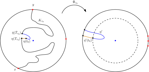
Figure 6.1: An illustration of the argument of Lemma 6.5 in the case $\{T^{\prime}<\infty\}$. The hull $K_{\tau_{0}}$ is shown in black. the curve $\eta^{\prime}$ and its pre-image under $\widetilde{\Phi}_{\tau_{0}}$ are shown in blue. The extra part of the curve which we grow after growing $K_{\tau_{0}}$ is shown in orange.

The following lemma is the main input in the proof of the lower bound in Proposition 6.1: it provides times $t_{0},\overline{t}_{0}>0$ for which $|\eta(t_{0})-\overline{\eta}(\overline{t}_{0})|$ is of order $e^{-\beta}$, the derivative of a conformal map $\mathbf{D}\setminus(\eta^{t_{0}}\cup\overline{\eta}^{\overline{t}_{0}})\rightarrow\mathbf{D}$ with the same normalization as $\phi_{\beta}$ is of order $e^{-\beta q}$, the points $\eta(t_{0})$ and $\overline{\eta}(\overline{t}_{0})$ are well separated in the harmonic measure sense, and the conditional law of the “middle” segment of $\eta$ given $\eta^{t_{0}}\cup\overline{\eta}^{\overline{t}_{0}}$ is that of an SLE_κ. Once we have these times, we just need to grow a little bit more of $\eta$ and $\overline{\eta}$ after times $t_{0}$ and $\overline{t}_{0}$, respectively, to get the estimate of Proposition 6.1.

Lemma 6.5.

Let $v>0$, $\zeta>0$, and $\mu_{0}\in\mathcal{M}$. For $\beta>0$ and two times $t,\overline{t}>0$, let $E_{\beta}^{0}(t,\overline{t})=E_{\beta}^{0}(t,\overline{t};v,\zeta,\mu_{0})$ be the event that the following occurs.

1. $32e^{-\beta}\leq\operatorname{dist}(0,\eta^{t}\cup\overline{\eta}^{\overline{t}})\leq e^{-\beta(1-v)}$.

2. Let $\phi_{t,\overline{t}}:\mathbf{D}\setminus(\eta^{t}\cup\overline{\eta}^{\overline{t}})\rightarrow\mathbf{D}$ be the conformal map which takes $x^{+}$ to $-i$, $y^{-}$ to $i$, and $m$ to 1. Then $e^{-\beta(q+v)}\leq|\phi_{t,\overline{t}}^{\prime}(0)|\leq e^{-\beta(q-v)}$.

3. Let $\psi_{t,\overline{t}}:\mathbf{D}\setminus(\eta^{t}\cup\overline{\eta}^{\overline{t}})\rightarrow\mathbf{D}$ be the conformal map which fixes $0$ and takes 1 to 1. Then $|\psi_{t,\overline{t}}(\eta(t))-\psi_{t,\overline{t}}(\overline{\eta}(\overline{t}))|\geq\zeta$.

4. $\mathcal{G}^{\prime}(\eta^{t}\cup\overline{\eta}^{\overline{t}},\mu_{0})$ occurs.

There is a deterministic $\zeta>0$ and $\mu_{0}\in\mathcal{M}$, independent of $v$ and $\beta$, such that for each $v>0$, there exists $\beta_{*}=\beta_{*}(v,\widetilde{d})>0$ such that for each $\beta\geq\beta_{*}$, there exist random times $t_{0}$ and $\overline{t}_{0}$ such that

$$\mathbf{P}(E_{\beta}^{0}(t_{0},\overline{t}_{0}))\succeq e^{-\beta(\gamma^{*}(q)+\gamma_{0}^{*}(q)v)},$$ (6.10)

where here $\gamma^{*}(q)$ and $\gamma_{0}^{*}(q)$ are as in Proposition 6.1 and the implicit constant is independent of $\beta$. Furthermore, we can choose $t_{0}$ and $\overline{t}_{0}$ in such a way that the conditional law given $\eta^{t_{0}}\cup\overline{\eta}^{\overline{t}_{0}}$ of the part of $\eta$ between $\eta(t_{0})$ and $\overline{\eta}(\overline{t}_{0})$ on the event $E_{\beta}^{0}(t_{0},\overline{t}_{0})$ is that of a chordal $\operatorname{SLE}_{\kappa}$ from $\eta(t_{0})$ to $\overline{\eta}(\overline{t}_{0})$ in $\mathbf{D}\setminus(\eta^{t_{0}}\cup\overline{\eta}^{\overline{t}_{0}})$.

Proof.

We will deduce the lemma from Theorem 4.1 and Lemma 6.4. Fix $v^{\prime}\in(0,v/4)$, to be chosen later in a manner depending only on $v$ and $q$, and let $s:=q/(q+1)$. If $\beta>0$ is chosen sufficiently small, in a manner depending only on $v^{\prime}$ and $q$, then we can find $\epsilon=\epsilon(s,v^{\prime},\beta)>0$ such that

$$\epsilon^{1-s}=e^{-\beta(1-o_{v^{\prime}}(1))}\quad\operatorname{and}\quad\epsilon^{1-s+2v^{\prime}}\geq 32e^{-\beta}.$$

Let $c>0$ and let $\mathcal{E}^{s;v^{\prime}}_{\epsilon}(\eta,0;c)$ be the event of Section 4.1 (with $v^{\prime}$ in place of $u$). Let $\Psi_{\eta}:D_{\eta}\rightarrow\mathbf{D}$ and $\Psi_{\eta}^{-}:D_{\eta}^{-}\rightarrow\mathbf{D}$ be as in that subsection. Let $\mu^{\prime}\in\mathcal{M}$ and let

$$\mathcal{E}:=\mathcal{E}^{s;v^{\prime}}_{\epsilon}(\eta,0;c)\cap\mathcal{G}(\Psi_{\eta},\mu^{\prime})\cap\mathcal{G}(\Psi_{\eta}^{-},\mu^{\prime}).$$

By Theorem 4.1, if the parameter $\mu^{\prime}$ is chosen appropriately (in a manner depending only on $q$) then we can find $\beta_{*}>0$ as in the statement of the lemma such that for each $\beta\geq\beta_{*}$,

$$\mathbf{P}(\mathcal{E})\succeq e^{-\beta(\gamma^{*}(q)+\gamma_{0}^{*}(q)v^{\prime})},$$

for an appropriate choice of $\gamma_{0}^{*}(q)$ as in Proposition 6.1. Lemma 2.8 implies that we can find $\mu_{0}\in\mathcal{M}$ depending only on $\mu^{\prime}$ such that

$$\mathcal{G}(\Psi_{\eta},\mu^{\prime})\cap\mathcal{G}(\Psi_{\eta}^{-},\mu^{\prime})\subset\bigcap_{t,\overline{t}\geq 0}\mathcal{G}^{\prime}(\eta^{t}\cup\overline{\eta}^{\overline{t}},\mu_{0}).$$ (6.11)

Let $\tau_{0}$ be the first time $\tau$ that the first two conditions in the definition of $E_{\beta}^{0}(T_{\tau},\overline{T}_{\tau})$ are satisfied and that $\widetilde{\Phi}_{\tau}(\eta(T_{\tau}))$ and $\widetilde{\Phi}_{\tau}(\overline{\eta}(\overline{T}_{\tau}))$ (as defined just above Lemma 6.2) both lie in $[i,-i]_{\partial\mathbf{D}}$. By Lemma 6.4 and the definition of $\mathcal{E}$, if $c$ is chosen sufficiently large then $\tau_{0}<\infty$ a.s. on $\mathcal{E}$. Moreover, decreasing $\tau$ only increases $\operatorname{hm}^{0}(\eta\setminus K_{\tau};D_{\eta})$, so on $\mathcal{E}$ a.s.

$$\operatorname{hm}^{0}(\eta\setminus K_{\tau_{0}};D_{\eta})\geq 1/4-o_{\beta}(1).$$ (6.12)

Let $\eta^{\prime}=\widetilde{\Phi}_{\tau_{0}}(\eta\setminus K_{\tau_{0}})$, with the parameterization it inherits from $\eta$. By the strong Markov property, the conditional law of $\eta^{\prime}$ given $K_{\tau_{0}}$ is that of a chordal $\operatorname{SLE}_{\kappa}$ from $x^{\prime}:=\widetilde{\Phi}_{\tau_{0}}(\eta(T_{\tau_{0}}))$ to $y^{\prime}:=\widetilde{\Phi}_{\tau_{0}}(\overline{\eta}(\overline{T}_{\tau_{0}}))$ in $\mathbf{D}$ (here we used that we made $\tau_{0}$ the smallest time for which our desired conditions are satisfied).

The definition, the event $E_{\beta}^{0}(t_{0},\overline{t}_{0})$ almost holds with $t_{0}=T_{\tau_{0}}$ and $\overline{t}_{0}=\overline{T}_{\tau_{0}}$, but $\widetilde{\Phi}_{\tau_{0}}(\eta(T_{\tau_{0}}))$ and $\widetilde{\Phi}_{\tau_{0}}(\overline{\eta}(\overline{T}_{\tau_{0}}))$ may be too close together. To this end, we will choose slightly larger times at which the images of the tips of $\eta$ and $\overline{\eta}$ are separated. Note that (6.12) implies $\operatorname{diam}\eta^{\prime}\geq\zeta_{0}$ on $\mathcal{E}$ for some universal constant $\zeta_{0}\in(0,1/4)$. Let $\overline{\eta}^{\prime}$ be the time reversal of $\eta^{\prime}$, with the parameterization it inherits from $\overline{\eta}$.

Let $T^{\prime}$ (resp. $\overline{T}^{\prime}$) be the first time that $\eta^{\prime}$ (resp. $\overline{\eta}^{\prime}$) enters $B_{1-\zeta_{0}/4}(0)$. Let $T^{\prime\prime}$ be the first time $t\geq T_{\tau_{0}}$ that $\operatorname{arg}\eta^{\prime}(t)\geq\operatorname{arg}x^{\prime}+\zeta_{0}/8$. Let $\overline{T}^{\prime\prime}$ be the first time $\overline{t}\geq\overline{T}_{\tau_{0}}$ that $\operatorname{arg}\overline{\eta}^{\prime}(\overline{t})\leq\operatorname{arg}y^{\prime}-\zeta_{0}/8$. Since $\operatorname{diam}\eta^{\prime}\geq\zeta_{0}$ a.s. on $\mathcal{E}$, either $|x^{\prime}-y^{\prime}|\geq\zeta_{0}/8$ or one of $T^{\prime},\overline{T}^{\prime},T^{\prime\prime}$ or $\overline{T}^{\prime\prime}$ is finite on this event (if not, then $\eta^{\prime}$ is contained in the wedge $\{z\in\mathbf{D}:\operatorname{arg}y^{\prime}-\zeta_{0}/8\leq\operatorname{arg}z\leq\operatorname{arg}x^{\prime}+\zeta_{0}/8,\>|z|\geq 1-\zeta_{0}/8\}$ and this wedge has diameter $<\zeta_{0}$). Hence the intersection with $\mathcal{E}$ of at least one of the events $\{|x^{\prime}-y^{\prime}|\geq\zeta_{0}/8\}$, $\{T^{\prime}<\infty\}$, $\{T^{\prime\prime}<T^{\prime}\}$, or $\{\overline{T}^{\prime\prime}<\overline{T}^{\prime}\}$ has probability at least $\frac{1}{4}\mathbf{P}(\mathcal{E})\succeq e^{-\beta(\gamma^{*}(q)+\gamma_{0}^{*}(q)v^{\prime})}$.

It is therefore enough to show that the conclusion of the lemma is true in each of the four possible cases (provided $\beta$ is sufficiently large). We will do this by choosing $t_{0}$ to be one of $T_{\tau_{0}},T^{\prime},$ or $T^{\prime\prime}$ and $\overline{t}_{0}$ to be one of $\overline{T}_{\tau_{0}},\overline{T}^{\prime}$, or $\overline{T}^{\prime\prime}$. By the strong Markov property, the last statement of the lemma holds for any such choice. Clearly, condition 1 in the definition of $E_{\beta}^{0}(t_{0},\overline{t}_{0})$ holds a.s. on $\mathcal{E}$ for any such choice of $t_{0}$ and $\overline{t}_{0}$ and any $v^{\prime}\in(0,v)$. By (6.11), condition 4 holds for any such choice. By conditions 1 and 2 in Lemma 6.4, on $\mathcal{E}$,

$$\frac{|\Phi_{\tau_{0}}^{\prime}(0)|}{|\Psi_{\eta}^{\prime}(0)|}\asymp 1\quad\operatorname{and}\quad\frac{\operatorname{dist}(0,K_{\tau_{0}})}{\operatorname{dist}(0,\eta)}\asymp 1$$

with deterministic, $\beta$-independent proportionality constants. By combining this with Lemma B.1 and condition 4 (c.f. Remark B.2), we infer that on $\mathcal{E}$,

$$\frac{\operatorname{hm}^{0}(I;D\setminus K_{\tau_{0}})}{\operatorname{hm}^{0}(I;D\setminus\eta)}\asymp 1,$$ (6.13)

for $I$ a sub-arc of $[-i,i]_{\partial\mathbf{D}}$ which is slightly smaller than $[-i,i]_{\partial\mathbf{D}}$. For any choice of $t_{0}$ and $\overline{t}_{0}$ as above, we have $K_{\tau_{0}}\subset(\eta^{\prime})^{t_{0}}\cup(\overline{\eta}^{\prime})^{\overline{t}_{0}}$. Since $4v^{\prime}<v$, (6.13) and a second application of Lemma B.1 yield condition 2 for large enough $\beta$.

Finally, we will verify that condition 3 holds in each of the four cases (for an appropriate choice of $\zeta>0$ depending only on $\zeta_{0}$). Here we note that $|x^{\prime}-y^{\prime}|$ is proportional to the harmonic measure from $0$ of the boundary arc of $\mathbf{D}\setminus((\eta^{\prime})^{t_{0}}\cup(\overline{\eta}^{\prime})^{\overline{t}_{0}})$ separating $\eta^{\prime}(t_{0})$ from $\overline{\eta}^{\prime}(\overline{t}_{0})$.

1. If $\mathbf{P}(|x^{\prime}-y^{\prime}|\geq\zeta_{0}/8,\>\mathcal{E})\succeq e^{-\beta(\gamma^{*}(q)+\gamma_{0}^{*}(q)v^{\prime})}$ then we can just set $t_{0}=T_{\tau_{0}}$, $\overline{t}_{0}=\overline{T}_{\tau_{0}}$, and $\zeta=\zeta_{0}/8$.

2. If $\mathbf{P}(T^{\prime}<\infty,\>\mathcal{E})\succeq e^{-\beta(\gamma^{*}(q)+\gamma_{0}^{*}(q)v^{\prime})}$ then we set $t_{0}=T^{\prime}$ and $\overline{t}_{0}=\overline{T}_{\tau_{0}}$. A Brownian motion has probability at least a constant $\zeta>0$ depending only on $\zeta_{0}$ to exit $B_{1-\zeta_{0}/16}(0)$ within distance $\zeta_{0}/4$ of 1 and then make a counterclockwise loop around the origin before leaving $\mathbf{D}\setminus B_{1-\zeta_{0}/8}(0)$. In this case it necessarily exits $\mathbf{D}\setminus(\eta^{\prime})^{T^{\prime}}$ on the left side of $(\eta^{\prime})^{T^{\prime}}$. See Figure 6.1 for an illustration in this case.

3. If $\mathbf{P}(T^{\prime\prime}<T^{\prime},\>\mathcal{E})\succeq e^{-\beta(\gamma^{*}(q)+\gamma_{0}^{*}(q)v^{\prime})}$ then we set $t_{0}=T^{\prime}\wedge T^{\prime\prime}$ and $\overline{t}_{0}=\overline{T}_{\tau_{0}}$. A Brownian motion has probability at least a constant $\zeta>0$ depending only on $\zeta_{0}$ to exit $\mathbf{D}$ before hitting any point outside of $\mathbf{D}\setminus B_{1-\zeta_{0}/8}(0)$ whose argument is not between $\operatorname{arg}x^{\prime}$ and $\operatorname{arg}x^{\prime}+\zeta_{0}/8$. If this is the case and $T^{\prime}\leq T^{\prime\prime}$, then a Brownian motion necessarily exits $\mathbf{D}\setminus(\eta^{\prime})^{t_{0}}$ on the left side of $(\eta^{\prime})^{t_{0}}$.

4. The case for $\{\overline{T}^{\prime\prime}<\overline{T}^{\prime}\}$ is treated in the same manner as the case for $\{T^{\prime\prime}<T^{\prime}\}$.

Thus we have exhausted all possible cases and we conclude that condition 3 holds. ∎

Proof of Proposition 6.1, lower bound.

Suppose $\zeta>0$, $\mu_{0}\in\mathcal{M}$, and random times $t_{0}$, $\overline{t}_{0}$ are chosen so that the conclusion of Lemma 6.5 holds. Let $v>0$ and let $\beta_{*}>0$ be chosen as in Lemma 6.5. Let $\beta\geq\beta_{*}$ and let $E_{\beta}^{0}=E_{\beta}^{0}(t_{0},\overline{t}_{0},v,\zeta,\mu_{0})$ be as in Lemma 6.5. We need to transfer the estimate of Lemma 6.5 from the setting when we stop at times $t_{0}$ and $\overline{t}_{0}$ to the setting when we stop at times $\tau_{\beta}$ and $\overline{\tau}_{\beta}$. The idea of the proof is to consider the hitting times of $\eta$ and $\overline{\eta}$ of logarithmically many balls centered at $0$ whose radii differ by an exponential factor and argue that at each scale, there is a positive probability that the curves continue to behave nicely. We then apply the strong Markov property and multiply over all of the scales.

To this end, let $\widetilde{\beta}=-\log\operatorname{dist}(0,\eta^{t_{0}}\cup\overline{\eta}^{\overline{t}_{0}})$. Note that on $E_{\beta}^{0}$,

$$\beta(1-v)\leq\widetilde{\beta}\leq\beta-\log 32.$$

Also fix $r\in(\log 16,\log 32)$. We will consider the hitting times of the balls $\mathcal{B}_{\widetilde{\beta}+kr}$ for $k\in\mathbf{N}$.

We start with the case $k=1$, which is slightly different. Let $\eta_{1}$ be the image under the map $\psi_{t_{0},\overline{t}_{0}}:\mathbf{D}\setminus(\eta^{t_{0}}\cup\overline{\eta}^{\overline{t}_{0}})\rightarrow\mathbf{D}$ which fixes $0$ (defined as in Lemma 6.5) of the part of $\eta$ between $\eta(t_{0})$ and $\overline{\eta}(\overline{t}_{0})$ and let $x_{1}$ and $y_{1}$ be its endpoints. Let $\tau_{1}^{\prime}$ (resp. $\overline{\tau}_{1}^{\prime}$) be the first time $\eta_{1}$ (resp. $\overline{\eta}_{1}$) hits $\psi_{t_{0},\overline{t}_{0}}(\mathcal{B}_{\widetilde{\beta}+r})$, so that $\psi_{t_{0},\overline{t}_{0}}(\eta(\tau_{\widetilde{\beta}+r}))=\eta_{1}(\tau_{1}^{\prime})$ and similarly for $\overline{\eta}$. Let $G_{1}$ be the event that the following holds.

1. $|\eta_{1}(\tau_{1}^{\prime})-\overline{\eta}_{1}(\overline{\tau}_{1}^{\prime})|\geq(1/32)e^{-r}$.

2. $\eta_{1}^{\tau_{1}^{\prime}}\cup\overline{\eta}_{1}^{\overline{\tau}_{1}^{\prime}}\subset\psi_{t_{0},\overline{t}_{0}}(\mathcal{B}_{1})$.

3. $\eta_{1}^{\tau_{1}^{\prime}}\cup\overline{\eta}_{1}^{\overline{\tau}_{1}^{\prime}}$ is disjoint from the $\zeta/2$-neighborhood of the segment connecting $0$ and the midpoint of the shorter arc between $x_{1}$ and $y_{1}$.

By the Koebe quarter theorem,

$$\mathcal{B}_{r+\log 16}\subset\psi_{t_{0},\overline{t}_{0}}(\mathcal{B}_{\widetilde{\beta}+r})\subset\mathcal{B}_{r-\log 16}.$$

Hence by Lemma 2.17, condition 3 in the definition of $E_{\beta}^{0}$, and the last statement of Lemma 6.5, $\mathbf{P}(G_{1}|E_{\beta}^{0})$ is at least a $\beta$-independent positive constant.

Now we consider the case $k\geq 2$. For $k=1,2,3,\ldots$, let $\widetilde{\psi}_{k}$ be the map from $\mathbf{D}\setminus(\eta^{\tau_{\widetilde{\beta}+kr}}\cup\overline{\eta}^{\overline{\tau}_{\widetilde{\beta}+kr}})$ to $\mathbf{D}$ with $\widetilde{\psi}_{k}(0)=0$ and $\widetilde{\psi}_{k}^{\prime}(0)>0$. For $k\geq 2$, let $\eta_{k}$ be the image under $\widetilde{\psi}_{k-1}$ of the part of $\eta$ which lies between $\eta(\tau_{\widetilde{\beta}+(k-1)r})$ and $\overline{\eta}(\overline{\tau}_{\widetilde{\beta}+(k-1)r})$. Then the law of $\eta_{k}$ given $\mathcal{F}_{\widetilde{\beta}+(k-1)r}$ (defined as in (6.5)) is that of a chordal $\operatorname{SLE}_{\kappa}$ from $x_{k}:=\widetilde{\psi}_{k-1}(\eta(\tau_{\widetilde{\beta}+(k-1)r}))$ to $y_{k}:=\widetilde{\psi}_{k-1}(\overline{\eta}(\overline{\tau}_{\widetilde{\beta}+(k-1)r}))$. Let $\overline{\eta}_{k}$ be the time reversal of $\eta_{k}$.

Let $\tau_{k}^{\prime}$ and $\overline{\tau}_{k}^{\prime}$ be the hitting times of $\widetilde{\psi}_{k-1}(\mathcal{B}_{\widetilde{\beta}+kr})$ by $\eta_{k}$ and $\overline{\eta}_{k}$, respectively, so that $\widetilde{\psi}_{k-1}(\eta(\tau_{\widetilde{\beta}+kr}))=\eta_{k}(\tau_{k}^{\prime})$ and similarly for $\overline{\eta}$. Fix $\delta>0$ and for $k\geq 1$ let $G_{k}$ be the event that $\eta^{\tau_{k}}$ (resp. $\overline{\eta}^{\overline{\tau}_{k}}$) is contained in the $\delta$-neighborhood of the segment $[x_{k},0]$ (resp. $[y_{k},0]$).

By the Koebe quarter theorem, whenever $\widetilde{\psi}_{k-1}$ is defined we have

$$\mathcal{B}_{r+\log 16}\subset\widetilde{\psi}_{k-1}(\mathcal{B}_{\widetilde{\beta}+kr})\subset\mathcal{B}_{r-\log 16}.$$

By conformal invariance of harmonic measure, on $G_{k-1}$ for $k\geq 2$, $|x_{k}-y_{k}|$ is at least a universal constant provided $\delta$ is taken sufficiently small. It now follows from Lemma 2.17 that for each $k\geq 2$,

$$\mathbf{P}\left(G_{k}\,|\,E_{\beta}^{0}\cap\bigcap_{j=1}^{k-1}G_{j}\right)\geq p$$ (6.14)

for some $p>0$ which depends only on $\delta$.

Let $k_{*}$ be the least integer $k$ such that $kr+\widetilde{\beta}\geq\beta$. Note that $k_{*}\leq\beta v/r$. Let

$$G^{*}:=\bigcap_{k=1}^{k_{*}}G_{k}.$$

We will now argue that $E_{\beta}^{0}\cap G^{*}\subset E$, then complete the proof by establishing an appropriate lower bound for $\mathbf{P}(E_{\beta}^{0}\cap G^{*})$ provided $v\ll u$ is chosen appropriately.

It is clear that on the event $E_{\beta}^{0}\cap G^{*}$, conditions 1, 3, and 4 in the definition of $E$ hold provided we take $\delta$ sufficiently small, depending on $a$. It remains to deal with condition 2. For $k\geq 1$, let $\widehat{\eta}_{k}$ be the curve obtained by connecting $\eta(\tau^{*}_{\widetilde{\beta}+kr})$ and $\overline{\eta}(\overline{\tau}^{*}_{\widetilde{\beta}+kr})$ via the arc of $\mathcal{B}_{\widetilde{\beta}+kr}$ which does not disconnect $0$ from $[x_{*},y_{*}]_{\partial\mathbf{D}}$. Let $\Psi_{\widehat{\eta}_{k}}$ be the conformal map from the connected component of $\mathbf{D}\setminus\widehat{\eta}_{k}$ containing $[x_{*},y_{*}]_{\partial\mathbf{D}}$ on its boundary to $\mathbf{D}$ which takes $x_{*}$ to $-i$, $y_{*}$ to $i$, and the midpoint of $[x_{*},y_{*}]_{\partial\mathbf{D}}$ to 1. By Lemma B.3,

$$C^{-1}|\Psi_{\widehat{\eta}_{k}}^{\prime}(0)|\leq|\phi_{\beta^{\prime}}^{\prime}(0)|\leq C|\Psi_{\widehat{\eta}_{k}}^{\prime}(0)|,\qquad\forall\beta^{\prime}\in[\widetilde{\beta}+(k-1)r,\widetilde{\beta}+kr],\qquad\forall k\geq 2$$ (6.15)

on $G^{*}$, for some deterministic $C>1$ depending only on $a$, $r$, and $\mu$. A similar statement holds for $k=1$ provided we replace $C$ with a constant $C_{1}>0$ which is allowed to depend on $\zeta$, but not $\beta$.

The estimate (6.15) implies in particular that $|\phi_{\widetilde{\beta}+(k-1)r}^{\prime}(0)|$ and $|\phi_{\widetilde{\beta}+kr}^{\prime}(0)|$ differ by a factor of at most $C^{2}$. Iterating (6.15) at most $\beta v/r$ times shows that on $G^{*}$,

$$C_{1}^{-1}C^{-2\beta v/r}e^{-\beta(q+v)}\leq|\phi_{\beta}^{\prime}(0)|\leq C_{1}C^{2\beta v/r}e^{-\beta(q-v)}.$$

If we choose $v$ such that $v\leq u/3$ and $C^{2v/r}\leq e^{(1\wedge\gamma_{0}^{*}(q))u/3}$ and $\beta$ sufficiently large that $C_{1}e^{\beta\gamma_{0}^{*}(q)u/3}\geq c$, then condition 2 in the definition of $E$ holds on $E_{\beta}^{0}\cap G^{*}$. By possibly further shrinking $v$, we can arrange that $p^{v/r}\leq e^{\gamma_{0}^{*}(q)u/2}$ where $p$ is the parameter from (6.14). From Lemma 6.5, our estimates for the conditional probabilities of the $G_{k}$’s, and our choice of parameters above,

$$\mathbf{P}(E)\geq\mathbf{P}(G_{1}|E_{0})p^{\beta v/r-1}e^{-\beta(\gamma^{*}(q)+\gamma_{0}^{*}(q)v)}\succeq e^{-\beta(\gamma^{*}(q)+\gamma_{0}^{*}(q)u)}.\qed$$

7 Two point estimate

7.1 Outline of the two-point estimate

The goal of this section is to prove our two-point estimate which will lead to a lower bound for the Hausdorff dimensions of the sets $\Theta^{s}(D_{\eta})$ and $\widetilde{\Theta}^{s}(D_{\eta})$ in Theorem 1.1. In particular, we will define events $E_{n}(z)$ for $z\in\mathbf{D}$ and $n\in\mathbf{N}$ and show that if $E_{n}(z)$ occurs for every $n\in\mathbf{N}$ (i.e., $z$ is a perfect point) then $z\in\Theta^{s}(D_{\eta})$; and that the correlation of $E_{n}(z)$ and $E_{n}(w)$ is small when $|z-w|$ is large, in a quantitative sense (Proposition 7.17). The proof of this latter correlation estimate uses the theory of imaginary geometry to get long-range independence for certain events.

Throughout this section, we will consider the following setup. Let $\chi=2/\sqrt{\kappa}-\sqrt{\kappa}/2$ and let $\lambda=\pi/\sqrt{\kappa}$ be the imaginary geometry parameters from (2.20). Let $h$ be a zero boundary GFF on $\mathbf{D}$ plus a harmonic function chosen in such a way that if $\psi:\mathbf{H}\rightarrow\mathbf{D}$ is the conformal map taking $0$ to $-i$, $\infty$ to $i$, and $i$ to $0$, then $h\circ\psi-\chi\operatorname{arg}\psi^{\prime}$ is a GFF on $\mathbf{H}$ with boundary data $-\lambda$ on $(-\infty,0]$ and $\lambda$ on $[0,\infty)$. By [MS16c, Theorem 1.1] the zero-angle flow line $\eta$ of $h$ started from $-i$ is a chordal $\operatorname{SLE}_{\kappa}$ from $-i$ to $i$ in $\mathbf{D}$. Let $\overline{\eta}$ be the time reversal of $\eta$. Also fix a multifractal spectrum parameter $s\in(-1,1)$ and let $q:=s/(1-s)\in(-1/2,\infty)$.

We will shortly give an outline of the content of the rest of this section, but before we do so we make some general comments about notation.

• We continue to use the notation $\mathcal{B}_{\beta}=B_{e^{-\beta}}(0)$ from (6.1). We also recall the notation $\eta^{\tau}=\eta([0,\tau])$ and we will always denote the time reversal of a curve by an overbar.

• All curves in this section are assumed to have some arbitrary parameterization. The times we consider will only be used to specify certain segments of the curve, and these segments will not depend on the choice of parameterization.

• The notation in the remainder of this section is quite heavy, but it is easier to navigate if the reader keeps in mind several conventions. Objects denoted with a superscript ${\operatorname{f}}$ are associated with the full curve $\eta$, as opposed to the curve $\eta_{z,j}$ at scale $j$. Conformal maps denoted by the symbol $\psi$ with some decoration map the complement of some part of $\eta$ (or a conformal image thereof) to $\mathbf{D}$ and are required to fix the origin. Conformal maps denoted by $\phi$ or $\Phi$ with some decoration map the complement of some segment of $\eta$ (or a conformal image thereof) to $\mathbf{D}$ and are specified by the images of three points on the boundary. Conformal maps denoted by $\pi$ with some decoration map a “pocket” formed by two auxiliary flow lines to $\mathbf{D}$. Conformal maps denoted by $f$ or $g$ with some decoration are automorphisms of $\mathbf{D}$.

• Much of the notation in this section is illustrated in Figures 7.1, 7.2, and 7.3 and summarized in Section 7.7.

We start in Section 7.2 by defining an event $E$ depending on parameters $\beta>0$ and $u\in(0,1)$ (which will eventually be sent to $0$ and $\infty$, respectively), a field $h$ on $\mathbf{D}$ with Dirichlet boundary data and its 0-angle flow line $\eta$ started from $x\in\partial\mathbf{D}$ to $y\in\partial\mathbf{D}$ (eventually, we will apply this definition inductively with $\eta$ replaced by the conformal image of a certain segment of our original SLE_κ curve $\eta$). The definition of $E$ also involves several constant-order auxiliary parameters which we list in Definition 7.1. Roughly speaking, $E$ is the event that the following hold.

1. If we run $\eta$ (resp. its time reversal) until the first time $\tau$ that it gets within distance $e^{-\beta}$ of the origin then apply a conformal map $\phi:\mathbf{D}\setminus(\eta^{\tau}\cup\overline{\eta}^{\overline{\tau}})\rightarrow\mathbf{D}$ normalized so that $\phi(x^{+})=-i$, $\phi(y^{-})=i$, and $\phi(\text{midpoint of $[x,y]_{\partial\mathbf{D}}$})=1$, then $|\phi^{\prime}(0)|$ is of order $e^{-\beta(q\pm u)}$.

2. Let $\eta^{-}$ and $\eta^{+}$ be flow lines of $h$ started from $\eta(\tau)$, with angles chosen so that they a.s. intersect each other. Then $\eta^{-}$ and $\eta^{+}$ form a “pocket” surrounding the origin with diameter of order $e^{-\beta}$ and a roughly round shape.

The first of these two conditions will ensure that the behavior of the derivative of a conformal map from one side of $\eta$ to $\mathbf{D}$ has the right derivative behavior and the second condition will allow us to get the long-range independence needed for our two-point estimate. We will also prove an estimate (Lemma 7.7) for the probability of $E$.

The actual definition of $E$ will involve several regularity conditions which are needed to rule out various types of pathological behavior. We will break the definition up into four steps which each serve a particular purpose in the proof of our two-point estimate. Let us now give a more detailed outline of each of these four steps and its purpose; see Figure 7.1 for an illustration of the definition and the objects involved.

The first step is to get away from the boundary so that our curve will look like an ordinary SLE_κ (even if it was originally an SLE${}_{\kappa}(\underline{\rho})$). We grow the curves $\eta$ and $\overline{\eta}$ up to times $\sigma$ and $\overline{\sigma}$, respectively, which are approximately equal to the first time these curves hit a certain ball centered at $0$ with small (but $\beta$-independent) size. Our first event $L$ is a list of regularity conditions for $\eta^{\sigma}$ and $\overline{\eta}^{\overline{\sigma}}$. The purpose of most of these conditions is to ensure that we can apply Lemma C.4 to get that the segment of $\eta$ from $\eta(\sigma)$ to $\overline{\eta}(\overline{\sigma})$ is close in law to an SLE_κ curve, even if $\eta$ is itself an SLE${}_{\kappa}(\rho^{L};\rho^{R})$ curve for $\rho^{L},\rho^{R}\in(-2,0)$. The probability of $L$ will be of constant order, independent of $\beta$ (Lemma 7.2). We note that the objects in the definition of $L$ are used infrequently outside the proof of Lemma 7.3.

The second step takes care of the derivative behavior; in particular, we let $\widetilde{E}$ be the event described in item 1 above, with the same regularity conditions appearing on the event of Proposition 6.1. The event $\widetilde{E}$ is the only event in the definition of $E$ whose conditional probability given the previous events is not of constant ($\beta$-independent) order; see Lemma 7.7 and Proposition 6.1.

Since the behavior of the derivative of a conformal map from the complement of $\eta$ to $\mathbf{D}$ can a priori depend on the whole curve $\eta$, we next introduce auxiliary flow lines $\eta^{\pm}$ to localize our events. These are flow lines of $h$ started from the point $\eta(\tau)$, with angles chosen so that they a.s. bounce off each other, but do not cross. We define an event $F$ which is the intersection of $\widetilde{E}$ and the event that these auxiliary flow lines make a pocket surrounding $0$ (which we call $D$) before hitting $\overline{\eta}^{\overline{\tau}}$ and satisfy certain regularity conditions.

The key property which these pockets $D$ satisfy, and which is the source of the long-range independence needed for our two-point estimate in Section 7.5, is that, conditional on a pocket, the restrictions of $h$ to the inside and outside of the pocket are conditionally independent (see Lemma 7.4). Since $h$ determines $\eta$ in a local manner, this will lead to independence between certain segments of $\eta$. The regularity conditions in the definition of $F$ govern the size and shape of the pocket $D$ and will be important in Section 7.4 when we compare derivatives of various conformal maps; and also ensure that the points where $\eta$ enters and exits the pocket are separated in the sense of harmonic measure from 0.

Finally, we define $E$ to be the intersection of $F$ and the event that $\eta$ and $\overline{\eta}$ do not have any pathological behavior between time they hit $\mathcal{B}_{\beta}$ and the time when they enter the pocket $D$.

In Section 7.3, we define events $E_{z,j}$ for $z\in\mathbf{D}$ and $j\in\mathbf{N}$ associated with our original field/curve pair $(h,\eta)$ as follows. Fix sequences $\beta_{j}\rightarrow\infty$ (at a logarithmic rate) and $u_{j}\rightarrow 0$ (at a very slow rate), which are chosen in Lemma 7.10. In the case $j=1$, we apply a conformal automorphism $f_{z,1}:\mathbf{D}\rightarrow\mathbf{D}$ sending $z$ to $0$ and let $E_{z,1}$ be the event $E$ of Section 7.2 defined with $\beta=\beta_{1}$, $u=u_{1}$, and $f_{z,1}\circ\eta_{z,1}$ in place of $\eta$. Inductively, for $j\geq 2$ we let $D_{z,j-1}$ be the pocket formed by the auxiliary flow lines used in the definition of $E_{z,j-1}$, let $\pi_{z,j-1}:D_{z,j-1}\rightarrow\mathbf{D}$ be a conformal map which fixes 0, let $E_{z,j}$ be the event $E$ of Section 7.2 with $\eta$ replaced by the image under $\pi_{z,j-1}$ of the segment of (a conformal image of) $\eta$ which is contained in $D_{z,j-1}$ and which $\beta=\beta_{j}$ and $u=u_{j}$. We then set

$$E_{n}(z):=\bigcap_{j=1}^{n}E_{z,j}$$

See Figure 7.2 for an illustration of the definitions of $E_{z,j}$ and $E_{n}(z)$.

In Section 7.4, we use a purely complex analytic argument to prove Lemma 7.13, which says that the derivatives of certain conformal maps and the diameters of certain sets are of the correct order on $E_{n}(z)$. This will be used in Section 8 to show that the perfect points (roughly speaking, those for which $E_{n}(z)$ occurs for every $n\in\mathbf{N}$) all belong to the multifractal spectrum set $\Theta^{s}(D_{\eta})$. The proofs in this subsection are perhaps the most technical ones in this section; the reader who wishes to see only the main ideas of the proof of our two-point estimate may wish to read Lemma 7.13, which is the only result from this subsection used in the rest of the proof, and skip the rest of Section 7.4.

In Section 7.5, we prove our two-point estimate Proposition 7.17 using the auxiliary flow lines in the definitions of our events and various conditioning arguments based on results from [MS16c]. The main idea of the proof is that (roughly speaking) the behavior of the field $h$, and hence also the curve $\eta$, inside the pockets $D_{z,n}^{\operatorname{f}}$ and $D_{w,n}^{\operatorname{f}}$ formed by the auxiliary flow lines is independent provided these pockets are disjoint, which allows us to get long-range independence for our events.

Section 7.6 contains a discussion about what adaptations one would make to our argument when proving two-point estimates for other sets associated with SLE.

For the convenience of the reader, we have included an index of the notation used in this section in Section 7.7.

7.2 Event for an SLE${}_{\kappa}(\rho^{L};\rho^{R})$ curve coupled with a GFF

Fix $\widetilde{d}>0$ and suppose $x,y\in\partial\mathbf{D}$ with $|x-y|\geq\widetilde{d}$. Also let $\rho^{L},\rho^{R}\in(-2,0]$ and let $h$ be a GFF on $\mathbf{D}$ with Dirichlet boundary data chosen in such a way that its 0-angle flow line $\eta$ from $x$ to $y$ is an SLE${}_{\kappa}(\rho^{L};\rho^{R})$ from $x$ to $y$, with force points located immediately to the left and right of $x$. Also fix $u\in(0,1)$ and $\beta>0$ (we will eventually send $u\rightarrow 0$ and $\beta\rightarrow\infty$).

All objects in this subsection are allowed to depend on $\rho^{L},\rho^{R}$, and $\kappa$ and we do not make this dependence explicit. We will, however, be careful about dependence on $x$ and $y$ which is why we introduce the parameter $\widetilde{d}$.

In this subsection, we will define an event $E$ associated with the curve $\eta$, the field $h$, the parameters $\beta$ and $u$, and several constant-order auxiliary parameters. We will also record an estimate for $\mathbf{P}(E)$. In the next subsection we will define the events $E_{z,j}$ and the associated objects by replacing $h$ with the conformal image of the restriction of $h$ to a sub-domain and replacing $\eta$ with the corresponding conformal image of a segment of $\eta$. See Figure 7.1 for an illustration of most of the objects defined in this subsection.

Definition 7.1 (Auxiliary parameters).

The auxiliary parameters are the objects $\Delta>\widetilde{\Delta}>1$, $\delta_{L},r,p_{L}\in(0,1)$, $a\in(0,1/4)$, and $\mu,\mu_{L},\mu_{F}\in\mathcal{M}$, all chosen in a manner which does not depend on $\beta$ or $u$.

The auxiliary parameters will be used in the definition of our events below and will be chosen in the following manner. In Lemma 7.7, we show that for a given choice of $r,a$, and $\widetilde{d}$, a certain estimate holds provided $\delta_{L}$, $p_{L}$, $\mu,\mu_{L},\mu_{F}$ are chosen sufficiently small, $\Delta$ and $\widetilde{\Delta}$ are chosen sufficiently large, and $\beta$ is large enough (depending on all of the auxiliary parameters). In Section 7.4, we make our choice of $r$. The parameter $a$ is allowed to remain arbitrary.

We now proceed with the definition of the event $E$, as outlined in Section 7.1. Let $\overline{\eta}$ be the time reversal of $\eta$. We first grow initial segments of $\eta$ and $\overline{\eta}$ in such a way that the “middle part” of $\eta$, between these two segments, looks like an ordinary SLE_κ.

Let $\sigma$ (resp. $\overline{\sigma})$ be the first time $\eta$ (resp. $\overline{\eta}$) hits $\mathcal{B}_{\Delta}$ (or $\infty$ if no such time exists). Let $[x^{*},y^{*}]_{\partial\mathbf{D}}$ be the largest sub-arc of $[x,y]_{\partial\mathbf{D}}$ which is not disconnected from the origin by $\eta^{\sigma}\cup\overline{\eta}^{\overline{\sigma}}$. Note that $x^{*}=x$ and $y^{*}=y$ if $\eta$ does not hit $\partial\mathbf{D}$ except at its endpoints (e.g., if $\eta$ is an ordinary SLE_κ).

Let $L$ be the event that the following occurs.

1. $\sigma,\overline{\sigma}<\infty$ and $\eta^{\sigma}$ (resp. $\overline{\eta}^{\overline{\sigma}}$) is contained in the $e^{-2\Delta}$-neighborhood of the segment $[x,0]$ (resp. $[y,0]$). Furthermore, $\eta$ (resp. $\overline{\eta}$) does not exit $\mathcal{B}_{\widetilde{\Delta}}$ between the first time it enters $\mathcal{B}_{\Delta/2}$ and time $\sigma$ (resp. $\overline{\sigma}$).

2. The harmonic measure from $0$ in $\mathbf{D}\setminus(\eta^{\sigma}\cup\overline{\eta}^{\overline{\sigma}})$ of each of the two sides of $\eta^{\sigma}$ and each of the two sides of $\overline{\eta}^{\overline{\sigma}}$ is at least $a$.

3. Let $\psi^{L}:\mathbf{D}\setminus(\eta^{\sigma}\cup\overline{\eta}^{\overline{\sigma}})\rightarrow\mathbf{D}$ be the conformal map with $\psi^{L}(0)=0$ and $(\psi^{L})^{\prime}(0)>0$. Then $(\psi^{L})^{-1}$ maps $B_{1-\mu(\delta_{L})}(0)\cup B_{\delta_{L}}(\psi^{L}(\eta(\sigma)))\cup B_{\delta_{L}}(\psi^{L}(\overline{\eta}(\overline{\sigma})))$ into $\mathcal{B}_{\widetilde{\Delta}}$.

4. $\mathcal{G}_{[x^{*},y^{*}]}(\psi^{L},\mu_{L})$ occurs (Definition 2.5).

5. The conditional probability given $\eta^{\sigma}\cup\overline{\eta}^{\overline{\sigma}}$ that the part of $\eta$ lying between $\eta(\sigma)$ and $\overline{\eta}(\overline{\sigma})$ never exits $\mathcal{B}_{\widetilde{\Delta}}$ is at least $p_{L}$.

See the middle panel of Figure 7.1 for an illustration. The main reason for most of the conditions in the definition of $L$ is so that the conditions of Lemma C.4 are satisfied, which will be used in Lemma 7.3 just below. The objects involved in the definition of $L$ ($\sigma$, $\overline{\sigma}$, $\psi^{L}$, etc.) are used infrequently in the rest of this section.

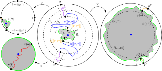
Figure 7.1: Illustration of the definition of the event $E$. Middle: The full curve $\eta$. The time segments of the curve involved in the definition of $L$ are shown in purple, those involved in the definition of $\widetilde{E}$ are shown in blue, and those involved in the last part of the definition of $E$ are shown in orange. The auxiliary flow lines $\eta^{\pm}$ involved in the definition of $F$ are shown in green. For clarity, the disks $\mathcal{B}_{\widetilde{\Delta}}$, $\mathcal{B}_{\Delta}$, and $\mathcal{B}_{\beta}$ here are shown larger than they actually are in practice. Top left: The image of the middle picture under the map $\phi:\mathbf{D}\setminus(\eta^{\tau}\cup\overline{\eta}^{\overline{\tau}})\rightarrow\mathbf{D}$. The derivative of this map at the origin is of order $e^{-\beta q}$ on $\widetilde{E}$. Bottom left: The image of the middle picture under the map $\pi:D\rightarrow\mathbf{D}$ with $\pi(0)=0$ and $\pi^{\prime}(0)>0$. In the setting of Section 7.3, if $\eta=\eta_{z,j}$, then the red curve in this picture is $\eta_{z,j+1}$. Right: The map $\psi$ takes $\mathbf{D}\setminus(\eta^{\tau}\cup\overline{\eta}^{\overline{\tau}})$ to $\mathbf{D}$ and fixes 0. The event $F$ includes several conditions which say that the flow lines $\psi(\eta^{\pm})$ behave nicely.

Lemma 7.2.

For each $\widetilde{d}\in(0,1)$, $\widetilde{\Delta}>0$, and $\mu\in\mathcal{M}$, it holds for sufficiently small $\delta_{L}\in(0,1)$, $\mu_{L}\in\mathcal{M}$, and $p_{L}\in(0,1)$ and sufficiently large $\Delta>\widetilde{\Delta}>1$, depending only on $\widetilde{d},\widetilde{\Delta}$, and $\mu$, that for each $a\in(0,1/4)$, we have $\mathbf{P}(L)\succeq 1$, with implicit constant depending on $\widetilde{d}$, $\rho^{L},\rho^{R},\kappa$, and the auxiliary parameters but uniform over all choices of endpoints $x,y$ with $|x-y|\geq\widetilde{d}$.

Proof.

This follows from Lemma 2.17. Note that we can apply the Koebe growth theorem to $(\psi^{L})^{-1}$ to find a $\delta_{L}=\delta_{L}(\widetilde{\Delta},\mu)>0$ so that the statement of the lemma holds, no matter how large we make $\widetilde{\Delta}$. ∎

We next define the “part” of the definition of $E$ which gives us control of the derivatives of certain conformal maps. This is the only event in this subsection which does not occur with constant-order (i.e., $\beta$-independent) conditional probability given the earlier events.

Recalling the auxiliary parameters from Definition 7.1, let $\widetilde{E}$ be the intersection of $L$ and the event $E_{\beta}^{q;u}(\eta;a,1,\mu)$ considered in Section 6, i.e., $\widetilde{E}$ is the event that the following is true.

1. The event $L$ defined above occurs. Moreover, let $\tau$ (resp. $\overline{\tau}$) be the first time $\eta$ (resp. $\overline{\eta}$) hits $\mathcal{B}_{\beta}$ (or $\infty$ if no such time exists). Then $\tau,\overline{\tau}<\infty$.

2. The conformal map $\phi:\mathbf{D}\setminus(\eta^{\tau}\cup\overline{\eta}^{\overline{\tau}})\rightarrow\mathbf{D}$ with $\phi(x^{+})=-i$, $\phi(y^{-})=i$, and $\phi(\text{midpoint of $[x,y]_{\partial\mathbf{D}}$})=1$ satisfies $e^{-\beta(q+u)}\leq|\phi^{\prime}(0)|\leq e^{-\beta(q-u)}$.

3. The harmonic measure from $0$ in $\mathbf{D}\setminus(\eta^{\tau}\cup\overline{\eta}^{\overline{\tau}})$ of each of the two sides of $\eta^{\tau}$ and each of the two sides of $\overline{\eta}^{\overline{\tau}}$ is at least $a$.

4. With $\psi^{L}$ as in condition 3 in the definition of $L$, the event $\mathcal{G}^{\prime}(\psi^{L}(\eta^{\tau}\cup\overline{\eta}^{\overline{\tau}}),\mu)$ occurs (Definition 2.6). .

The event $\widetilde{E}$ is illustrated in the middle panel of Figure 7.1.

We now record our estimate for $\mathbf{P}(\widetilde{E})$.

Lemma 7.3.

There exists $u_{*}=u_{*}(q)\in(0,1)$ such that for each $u\in(0,u_{*}]$ and each $\widetilde{d}\in(0,1)$, it holds for sufficiently small $\delta_{L}\in(0,1)$, $\mu,\mu_{L}\in\mathcal{M}$, and $p_{L}\in(0,1)$ and sufficiently large $\Delta>\widetilde{\Delta}$, depending only on $\widetilde{d}$, and all $a\in(0,1/4)$ that the following is true. There exists $\beta_{*}>0$ (depending on $u$, $\widetilde{d}$, and the auxiliary parameters) such that for $\beta\geq\beta_{*}$,

$$e^{-\beta(\gamma^{*}(q)+\gamma_{0}^{*}(q)u)}\leq\mathbf{P}\left(\widetilde{E}\right)\leq e^{-\beta(\gamma^{*}(q)-\gamma_{0}^{*}(q)u)}$$ (7.1)

where here $\gamma^{*}(q)$ and $\gamma_{0}^{*}(q)$ are the exponents from Proposition 6.1 and the implicit constants depend on $u$, $\widetilde{d}$, and the auxiliary parameters.

Due to the Markov property and reversibility of SLE_κ, Lemma 7.3 is almost immediate from Lemma 7.2 and Proposition 6.1 if $\rho^{L}=\rho^{R}=0$. In order to treat the case of general $\rho^{L},\rho^{R}\in(-2,0]$, we will use an absolute continuity argument based on the result of Appendix C since Proposition 6.1 is only proven for $\rho^{L}=\rho^{R}=0$.

Proof of Lemma 7.3.

Let $\psi^{L}:\mathbf{D}\setminus(\eta^{\sigma}\cup\overline{\eta}^{\overline{\sigma}})\rightarrow\mathbf{D}$ be the conformal map from condition 3 in the definition of the event $L$. Define the curve $\eta_{0}:=\psi^{L}(\eta\setminus(\eta^{\sigma}\cup\overline{\eta}^{\overline{\sigma}}))$. Also let $H^{*}:=\left\{\eta\setminus(\eta^{\sigma}\cup\overline{\eta}^{\overline{\sigma}})\subset\mathcal{B}_{\widetilde{\Delta}}\right\}$, as in Appendix C. By condition 3 in the definition of $L$ and condition 4 in the definition of $\widetilde{E}$, we infer that $\widetilde{E}\subset H^{*}$.

By conditions 1 and 5 in the definition of $L$, this event is contained in the event $S$ of Lemma C.4. By Lemma C.4, if $\widetilde{\Delta}$ (and hence also $\Delta$) is chosen sufficiently large, then the regular conditional law of the curve $\eta_{0}$ given $\eta^{\sigma}\cup\overline{\eta}^{\overline{\sigma}}$ and the event $H^{*}$ on the event $L$ is strictly mutually absolutely continuous (s.m.a.c.; Definition C.1) with respect to the law of a chordal SLE_κ from $\psi^{L}(\eta(\sigma))$ to $\psi^{L}(\overline{\eta}(\overline{\sigma}))$ in $\mathbf{D}$ conditioned to stay in $\psi^{L}(\mathcal{B}_{\widetilde{\Delta}})$, with implicit constants depending only on $\widetilde{d}$, $\rho^{L},\rho^{R},\kappa$, and the auxiliary parameters. By condition 5 in the definition of $L$, the same is true of the regular conditional law of $\eta_{0}$ given $\eta^{\sigma}\cup\overline{\eta}^{\overline{\sigma}}$ on the event $L$ restricted to the event $H^{*}$. By condition 5 in the definition of $L$, $\mathcal{G}(\eta_{0},\mu)\subset H^{*}$.

By condition 2 in the definition of $L$, $|\psi^{L}(\eta(\sigma))-\psi^{L}(\overline{\eta}(\overline{\sigma}))|$ is bounded below by a positive $a$-dependent constant on $L$. By this, Proposition 6.1, and the absolute continuity considerations in the preceding paragraph, we find that (in the notation of Proposition 6.1) for an appropriate choice of $u_{*}\in(0,1)$ and a small enough choice of $\mu\in\mathcal{M}$, it holds on $L$ that for each $u\in(0,u_{*}]$ and $c>0$, there exists $\widetilde{\beta}_{*}=\widetilde{\beta}_{*}(u,a,c)>0$ such that for $\widetilde{\beta}\geq\widetilde{\beta}_{*}$, the conditional probability of the event of Proposition 6.1 on $L$ a.s. satisfies

$$e^{-\widetilde{\beta}(\gamma^{*}(q)+\gamma_{0}^{*}(q)u)}\leq\mathbf{P}\left(E_{\widetilde{\beta}}^{q;u}(\eta_{0};a,c,\mu)\,|\,\eta^{\sigma}\cup\overline{\eta}^{\overline{\sigma}}\right)\leq e^{-\widetilde{\beta}(\gamma^{*}(q)-\gamma_{0}^{*}(q)u)}.$$ (7.2)

Note that if $\mu$ is chosen sufficiently small, then $E_{\widetilde{\beta}}^{q;u}(\eta_{0};a,c,\mu)\subset H^{*}$ by condition 3 in the definition of $L$. By the Koebe quarter theorem, we can find $C>0$ depending only on $\Delta$ such that on $L$,

$$\mathcal{B}_{\beta+C}\subset\psi^{L}(\mathcal{B}_{\beta})\subset\mathcal{B}_{\beta-C}.$$ (7.3)

It is clear from Lemma 2.17, the above absolute continuity statement, and the Markov property of ordinary SLE_κ that for an appropriate choice of $c=c(\Delta)\in(0,1)$, the conditional probability of $\widetilde{E}$ given $\eta^{\sigma}\cup\overline{\eta}^{\overline{\sigma}}$ and the event $E_{\beta-C}^{q;u}(\eta_{0};a,c,\mu)$; and the conditional probability of $E_{\beta+C}^{q;u}(\eta_{0};a,c^{-1},\mu)$ given $\eta^{\sigma}\cup\overline{\eta}^{\overline{\sigma}}$ and the event $\widetilde{E}$ are each a.s. bounded below by positive deterministic constants depending only on $\widetilde{d}$ and the auxiliary parameters. Combining this with (7.2) and Lemma 7.2 yields the statement of the lemma with $\beta_{*}=\widetilde{\beta}_{*}+C$. ∎

We next define auxiliary flow lines $\eta^{\pm}$ started from $\eta(\tau)$ which form a “pocket” surrounding $0$ with size of order $e^{-\beta}$ with uniformly positive probability. The reason for introducing these flow lines is as follows. Roughly speaking, the part of $\eta$ inside $D$ is conditionally independent of the part of $\eta$ which outside $D$ given the flow lines $\eta^{\pm}$ (see Lemma 7.4 below). When applied at various scales, this fact will eventually allow us to get the needed long-range independence for our two-point estimate.

Fix $\theta>0$, to be chosen momentarily, in a manner depending only on $\kappa$. On $\widetilde{E}$, let $\eta^{-}$ and $\eta^{+}$ be the flow lines of $h$ started from $\eta(\tau)$ with angles $\theta$ and $-\theta$, respectively. Note that the flow line with a negative sign has positive angle and vice versa. This is because a flow line with a negative angle a.s. stays to the right of $\eta$, and a flow line with a positive angle a.s. stays to the left of $\eta$. See [MS16c, Theorem 1.5].

By examining the boundary data of the field $h$ along $\eta$ and applying [MS16c, Theorems 1.1 and 2.4], we find that the conditional law of $\eta^{-}$ (resp. $\eta^{+}$) given $\eta$ on the event $\{\tau<\infty\}$ is that of a certain $\operatorname{SLE}_{\kappa}(\underline{\rho})$ process from $\eta_{0}(\tau)$ to $i$ in the right (resp. left) connected component of $\mathbf{D}\setminus\eta_{0}$, with force points immediately the the left and right of its starting point and at the endpoints $x$ and $y$. The weights of the force points immediately to the left and right of the starting point are given by

$$\rho^{0}=-\frac{\theta\chi}{\lambda}\quad\operatorname{and}\quad\rho^{1}=\frac{\theta\chi}{\lambda}-2,$$ (7.4)

with $\rho^{0}$ the force point on the side corresponding to $\eta^{\tau}$. (See [MS16c, Section 2.2] for a discussion and rigorous construction of SLE${}_{\kappa}(\rho^{0};\rho^{1})$ with force points immediately to the left and right of the starting point).

By [MS16c, Theorem 1.5, assertion (iii)], $\eta^{\pm}$ a.s. intersect (but do not cross) each other provided $\theta<\pi\kappa/(4-\kappa)$. By [MS16c, Remark 5.3], $\eta^{\pm}$ a.s. do not hit $\eta^{\tau}$ provided $-\theta\chi/\lambda\geq\kappa/2-2$. Hence we can choose $\theta>0$ sufficiently small, depending only on $\kappa$ in such a way that $\eta^{\pm}$ a.s. intersect each other and a.s. do not hit $\eta^{\tau}$. We henceforth assume that $\theta$ has been chosen in this manner.

If there is a connected component of $\mathbf{D}\setminus(\eta^{-}\cup\eta^{+})$ lying between $\eta^{-}$ and $\eta^{+}$ which contains 0, we take $D$ to be this connected component, and we set $D=\emptyset$ otherwise. We also let $\pi:D\rightarrow\mathbf{D}$ be the conformal map with $\pi(0)=0$ and $\pi^{\prime}(0)>0$.

The next piece in the definition of our event $E$ is a list of regularity conditions for the flow lines $\eta^{\pm}$ which ensures that the pocket $D$ they form has a roughly round shape. Let $t^{+}$ be the first time that $\eta^{+}$ hits $\eta^{-}$ after the first time it exits the disk of radius $e^{-\beta-1}$ centered at $\eta(\tau)$. Let $t^{-}$ be the time such that $\eta^{-}(t^{-})=\eta^{+}(t^{+})$. Let $\overline{b}=\eta^{-}(t^{-})=\eta^{+}(t^{+})$ and let $b$ be the last intersection point of $\eta^{\pm}$ before hitting $\overline{b}$, so that if $D\not=\emptyset$, then $b$ and $\overline{b}$ are the first and last points of $\partial D$ hit by $\eta^{\pm}$. Also let $\widetilde{t}^{\pm}$ be the first exit times of $\eta^{\pm}$ from the annulus $\mathcal{B}_{\beta-\Delta}\setminus\mathcal{B}_{\beta+\Delta}$. Let $F$ be the event that the following occurs.

1. $\widetilde{E}$ occurs, $t^{+}\leq\widetilde{t}^{+}$, $t^{-}\leq\widetilde{t}^{-}$, $D\not=\emptyset$, and $\overline{b}\notin\overline{\eta}^{\overline{\tau}}$.

2. Let $\psi:\mathbf{D}\setminus(\eta^{\tau}\cup\overline{\eta}^{\overline{\tau}})$ be the conformal map with $\psi(0)=0$ and $\psi^{\prime}(0)>0$. Let $x^{F}=\psi(\eta(\tau))$ and $y^{F}=\psi(\overline{\eta}(\overline{\tau}))$. Then $|\psi(b)-x^{F}|$ and $|\psi(\overline{b})-y^{F}|$ are each at most $r$.

3. Each point of $\psi((\eta^{+})^{t^{+}})$ (resp. $\psi((\eta^{-})^{t^{-}})$) lies within distance $r$ of $[x^{F},y^{F}]_{\partial\mathbf{D}}$ (resp. $[y^{F},x^{F}]_{\partial\mathbf{D}}$).

4. $\mathcal{G}^{\prime}(\psi((\eta^{+})^{t^{+}}\cup(\eta^{-})^{t^{-}}),\mu^{F})$ occurs (Definition 2.6).

See the right panel in Figure 7.1 for an illustration of the event $F$.

The main reason for our interest in the domain $D$ is contained in the following lemma, which will be a key tool in our two-point estimate.

Lemma 7.4.

Recall the pocket $D$ formed by the auxiliary flow lines $\eta^{\pm}$ and its two marked boundary points $b$ and $\overline{b}$. On the event $\{D\not=\emptyset\}$, if we condition on $D$ and $h|_{\mathbf{D}\setminus D}$ then the joint conditional law of $h|_{D}$ and the segment of $\eta$ contained in $\overline{D}$ is that of a GFF with Dirichlet boundary data determined by $(D,b,\overline{b})$ and its zero-angle flow line from $b$ to $\overline{b}$. In particular, the conditional law of this segment of $\eta$ given $D$ and $h|_{\mathbf{D}\setminus D}$ is that of a chordal $\operatorname{SLE}_{\kappa}(\rho^{1};\rho^{1})$ in $D$ from $b$ to $\overline{b}$, with $\rho^{1}$ as in (7.4).

Proof.

By [MS16c, Theorem 1.1] and since $\tau$ is a stopping time for $\eta$, the set

$$A:=\eta^{\tau}\cup\eta^{-}\cup\eta^{+}$$

is a local set for $h$ in the sense of [SS13, Section 3.3], i.e., the conditional law of $h|_{\mathbf{D}\setminus A}$ given $A$ and $h|_{A}$ is that of an independent zero-boundary GFF in each connected component of $\mathbf{D}\setminus A$ plus a harmonic function determined by $(h|_{\mathbf{D}\setminus A},A)$. This harmonic function is described explicitly in [MS16c, Theorem 1.1]: in particular, the conditional law of $h|_{D}$ given $(A,h|_{D\setminus A})$ on the event $\{D\not=\emptyset\}$ is that of a GFF on $D$ with boundary data $\lambda-\theta\chi-\chi\cdot\operatorname{winding}$ on $[\overline{b},b]_{\partial D}$ and $-\lambda+\theta\chi-\chi\cdot\operatorname{winding}$ on $[b,\overline{b}]_{\partial D}$, where $\lambda$ and $\chi$ are as in Section 2.5 and the term “winding” has the meaning of [MS16c, Figure 1.9].

The domain $D$ is one of the connected components of $\mathbf{D}\setminus A$ and the field $h|_{\mathbf{D}\setminus D}$ is determined by $A$, $h|_{A}$, and the restrictions of $h$ to the other connected components of $\mathbf{D}\setminus A$. Since $A$ is a local set for $h$ and is a.s. determined by $h$ (by [MS16c, Theorem 1.2]), we infer that $A$ is a.s. determined by $D$ and $h|_{\mathbf{D}\setminus A}$. Hence we get the same conditional law for $h|_{D}$ if we instead condition on $D$ and $h|_{\mathbf{D}\setminus D}$.

The statement about the conditional law of the segment of $\eta$ contained in $\overline{D}$ follows easily from our description of the conditional law of $h|_{D}$ and [MS16c, Theorems 1.1 and 2.4]. ∎

To complete the definition of our event $E$, we need one last regularity condition to rule out pathological behavior of the segments of $\eta$ and $\overline{\eta}$ before they hit $D$. Let $\tau^{*}$ (resp. $\overline{\tau}^{*}$) be the time at which $\eta$ (resp. $\overline{\eta}$) hits $b$ (resp. $\overline{b}$). Note that these times are a.s. finite if $F$ occurs since $\eta^{-}$ and $\eta^{+}$ a.s. lie to the left and right of $\eta$, respectively. Let $E$ be the event that the following occurs.

1. $F$ occurs.

2. With $\psi$ as in condition 2 in the definition of $F$, $\psi(\eta_{0}([\tau,\tau^{*}]))$ (resp. $\psi(\overline{\eta}_{0}([\overline{\tau},\overline{\tau}^{*}])$) is contained in the disk of radius $2r$ centered at $x^{F}$ (resp. $y^{F}$) (notation as in condition 2 in the definition of $F$).

Remark 7.5.

By [MS16c, Theorem 1.5] $\eta$ cannot cross $\eta^{\pm}$. By combining this with condition 3 in the definition of $L$, condition 4 in the definition of $\widetilde{E}$, and condition 2 in the definition of $E$, it follows that the segment of $\eta$ between $\eta(\sigma)$ and $\overline{\eta}(\overline{\sigma})$) is contained in $\mathcal{B}_{\widetilde{\Delta}}$ on the event $E$.

We now estimate the conditional probability of $E$ given the second intermediate event $\widetilde{E}$ defined above.

Lemma 7.6.

For each $r\in(0,1/2)$, it holds for sufficiently small $\mu_{F}\in\mathcal{M}$ and sufficiently large $\Delta>1$, depending only on $r$, $a$, and $\widetilde{d}$, that $\mathbf{P}(E\,|\,\widetilde{E})\succeq 1$, with the implicit constant depending only on $\widetilde{d}$ and the auxiliary parameters.

Proof.

Let $\eta^{F}$ be the image under $\psi$ of the part of $\eta$ between $\eta(\tau)$ and $\overline{\eta}(\overline{\tau})$. Note that the distance between the endpoints $x^{F}$ and $y^{F}$ of $\eta^{F}$ is uniformly positive on $\widetilde{E}$ by condition 3 in the definition of $\widetilde{E}$.

Let $\widetilde{r}\in(0,r^{2})$ and let $U$ be the $\widetilde{r}$-neighborhood of the line segment from $x^{F}$ to $y^{F}$. Also let $\mu_{F}^{\prime}\in\mathcal{M}$ and let $S$ be the event that $\eta^{F}\subset U$, $\mathcal{G}^{\prime}(\eta^{F},\mu_{F}^{\prime})$ occurs, and the time reversal of $\eta^{F}$ does not enter $B_{\widetilde{r}}(y^{F})$ after leaving $B_{2\widetilde{r}}(y^{F})$.

The absolute continuity considerations in the proof of Lemma 7.3 (still applied at times $\sigma$ and $\overline{\sigma}$) show that the conditional law of $\eta^{F}$ given $\eta^{\tau}\cup\overline{\eta}^{\overline{\tau}}$ on the event $\widetilde{E}$, restricted to the event $S$, is s.m.a.c. with respect to the law of a chordal SLE_κ from $x^{F}$ to $y^{F}$ in $\mathbf{D}$, with implicit constants depending only on $\widetilde{d}$, $\rho^{L},\rho^{R},\kappa$, and the auxiliary parameters. By Lemma 2.17, we infer that $\mathbf{P}(S\,|\,\widetilde{E})\succeq 1$.

The conditional law of $\psi(\eta^{+})$ given $\eta$ on the event $\widetilde{E}\cap S$ is that of an SLE${}_{\kappa}(\underline{\rho})$ process in the right connected component of $\mathbf{D}\setminus\eta^{F}$ from $x^{F}$ to $\psi(i^{-})$; it has force points with weights (7.4) on either side of its starting point, and two other boundary force points lying at uniformly positive distance from its start and end points (this distance it uniformly positive by condition 3 in the definition of $\widetilde{E}$). Similar statements hold with $-$ in place of $+$ and “left” in place of “right”. By Lemma 2.18 and the Beurling estimate (to make sure that $\psi(\mathcal{B}_{\beta+\Delta})$ covers most of $\mathbf{D}$) we infer that $\mathbf{P}(E\,|\,\widetilde{E}\cap S)\succeq 1$ provided $\mu_{F}$ is chosen sufficiently small and $\Delta>1$ is chosen sufficiently large, in a manner depending only on $r$. Since $\widetilde{r}<r$, if $F\cap\widetilde{E}\cap S$ occurs, then so does $E$. We conclude by observing that

$$\mathbf{P}\left(E\,|\,\widetilde{E}\right)\geq\mathbf{P}\left(E\cap S\,|\,\widetilde{E}\right)=\mathbf{P}\left(E\,|\,\widetilde{E}\cap S\right)\mathbf{P}\left(S\,|\,\widetilde{E}\right).\qed$$

By combining Lemmas 7.3 and 7.6, we infer the following one-point estimate for the event $E$.

Lemma 7.7.

Let $\widetilde{d}\in(0,1)$ and $a,r\in(0,1/4)$. There exists $u_{*}=u_{*}(q)\in(0,1)$ such that the following is true for each $u\in(0,u_{*}]$. If we choose $\delta_{L},p_{L}$, $\mu,\mu_{L},$ and $\mu_{F}$ sufficiently small, and $\Delta>\widetilde{\Delta}$ sufficiently large in a manner depending only on $\widetilde{d}$, $a$, and $r$, then we can find $\beta_{*}(u)>0$ (depending on $u$, $\widetilde{d}$, and the auxiliary parameters) such that for $\beta\geq\beta_{*}(u)$,

$$e^{-\beta(\gamma^{*}(q)+\gamma_{0}^{*}(q)u)}\preceq\mathbf{P}(E)\preceq e^{-\beta(\gamma^{*}(q)-\gamma_{0}^{*}(q)u)}$$

with the implicit constants depending only on $u$, $\widetilde{d}$, and the auxiliary parameters.

The last lemma in this subsection will be used to circumvent the fact that the laws of our objects will not be exactly the same at every scale. To explain this, we observe that Lemma 7.4 gives the objects defined in this subsection a certain self-similarity property: if $E$ occurs and we replace $(h,\eta)$ with the pushforward under the map $\pi:D\rightarrow\mathbf{D}$ of $(h|_{D},\eta\setminus(\eta^{\tau^{*}}\cup\overline{\eta}^{\overline{\tau}^{*}})$ then we end up in the same situation we started with but with $(\rho^{1},\rho^{1})$ in place of $(\rho^{L},\rho^{R})$ and a possibly different choice of start and end points for the curve. If we start with $\rho^{L}=\rho^{R}=\rho^{1}$, then we can remove the lack of stationarity coming from the change of $\rho$-values. The asymmetry coming from the change of start and end points is non-trivial, and is dealt with in the following lemma. We note that by rotational invariance, we only care about $\operatorname{arg}(y/x)$, not the particular values of $x$ and $y$.

Lemma 7.8.

Let $r_{H}>0$ and let $H=H(a,r_{H})$ be the event that the following is true.

1. With $\tau$ as in condition 1 in the definition of $\widetilde{E}$, we have $\tau<\infty$ and the harmonic measure from $0$ in $\mathbf{D}\setminus\eta^{\tau}$ of each side of $\eta^{\tau}$ is at least $a$.

2. Let $\psi^{H}:\mathbf{D}\setminus\eta^{\tau}\rightarrow\mathbf{D}$ be the conformal map with $\psi^{H}(0)=0$ and $\psi^{H}(\eta(\tau))=-i$. Then each point of $\psi^{H}(\partial D)$ lies at distance at least $r_{H}$ from $\partial\mathbf{D}\setminus B_{a}(-i)$.

Recalling the map $\pi:D\rightarrow\mathbf{D}$ which fixes 0, let $x^{\prime}:=\pi(b)$ and $y^{\prime}:=\pi(\overline{b})$, so that $x^{\prime}$ and $y^{\prime}$ are the start and end points of the image under $\pi$ of the segment of $\eta$ contained in $\overline{D}$. Suppose also that we are given two choices of start/end point pairs $(x_{1},y_{1})$ and $(x_{2},y_{2})$ for $\eta$ with $|x_{1}-y_{1}|,|x_{2}-y_{2}|\geq\widetilde{d}$, and for $i\in\{1,2\}$ denote the objects defined above with $(x_{i},y_{i})$ in place of $(x,y)$ with a subscript $i$. The conditional law of $\operatorname{arg}(y_{1}^{\prime}/x_{1}^{\prime})$ given $H_{1}$ and the conditional law of $\operatorname{arg}(y_{2}^{\prime}/x_{2}^{\prime})$ given $H_{2}$ are strictly mutually absolutely continuous (s.m.a.c.; Definition C.1), with the implicit constant depending only on $\widetilde{d}$, $a$, and $r_{H}$ (not on $\beta$, $u$, or the particular choice of $(x_{1},y_{1})$ and $(x_{2},y_{2})$).

With $H$ the event of Lemma 7.8, it follows from condition 3 in the definition of $\widetilde{E}$, condition 4 in the definition of $F$, and the Schwarz lemma applied to the map $\psi\circ(\psi^{H})^{-1}:\mathbf{D}\setminus\psi^{H}(\overline{\eta}^{\overline{\tau}})\rightarrow\mathbf{D}$ that for any choice of the auxiliary parameters $a\in(0,1/4)$ and $\mu_{F}\in\mathcal{M}$, there is an $r_{H}=r_{H}(a,\mu_{F})$ for which $E\subset H$.

Proof of Lemma 7.8.

We observe that $\operatorname{arg}(y^{\prime}/x^{\prime})$ is equal to $2\pi$ times the harmonic measure from $0$ of $\partial D\cap\eta^{+}$. Hence we need to prove an absolute continuity statement for this harmonic measure.

The conditional law of the curve $\psi^{H}(\eta^{-})$ (resp. $\psi^{H}(\eta^{+})$) given $\eta^{\tau}$ is that of a certain chordal SLE${}_{\kappa}(\underline{\rho})$ (resp. SLE${}_{\kappa}(\underline{\rho})$) from $-i$ to $\psi^{H}(i)$ in $\mathbf{D}$ with force points of weight $\rho^{1}$ (as in (7.4)) and $\theta\chi/\lambda$ located on either side of $-i$ and additional force points located at $\psi^{H}(x^{-})$ and $\psi^{H}(x^{+})$. By condition 1 in the definition of $H$, on $H$ each of these additional force points lies at distance at least $2a$ from $-i$.

Let $U$ be the set of points in $\mathbf{D}$ which lie at distance at least $r_{H}$ from $\partial\mathbf{D}\setminus B_{a}(-i)$ and let $t^{U,\pm}$ be the exit time of $\eta^{\pm}$ from $U$. By [MW17, Lemma 2.8] (applied once to $\eta^{-}$ and once to the conditional law of $\eta^{+}$ given $\eta^{-}$) we infer that, in the notation of the lemma, the joint conditional law of $((\eta_{1}^{-})^{t_{1}^{U,-}},(\eta_{1}^{+})^{t_{1}^{U,+}})$ given $\eta_{1}^{\tau_{1}}$ on the event that condition 2 in the definition of $H_{1}$ holds; and the joint conditional law of $((\eta_{2}^{-})^{t_{2}^{U,-}},(\eta_{2}^{+})^{t_{2}^{U,+}})$ given $\eta_{2}^{\tau_{2}}$ on the event that condition 2 in the definition of $H_{2}$ holds; are s.m.a.c., with implicit constants depending only on $\widetilde{d}$, $a$, and $r_{H}$. This immediately implies the statement of the lemma. ∎

7.3 Events for the perfect points

Recall the setting described at the beginning of Section 7.1: $h$ is a GFF on $\mathbf{D}$ with Dirichlet boundary data chosen so that its 0-angle flow line $\eta$ from $-i$ to $i$ is an ordinary SLE_κ.

Fix auxiliary parameters $r,a$ (to be chosen later) and assume that the other auxiliary parameters from Definition 7.1 are chosen in such a way that the conclusion of Lemma 7.7 holds for this choice of $r$ and $a$.

Fix $d\in(0,1)$; we will work on $B_{d}(0)$ to avoid pathologies coming from the boundary. Also fix sequences of positive numbers $\beta_{j}\rightarrow\infty$ and $u_{j}\rightarrow 0$ to be chosen in Lemma 7.10 just below; we note that in particular $\beta_{j}$ will grow like $\log j$.

In this subsection we will define the main events and objects we consider in the rest of this section using the construction of Section 7.2 and induction over scales of size $e^{-\beta_{j}}$. See Figure 7.2 for an illustration of the objects defined in this subsection and Section  7.7 for an index of these objects.

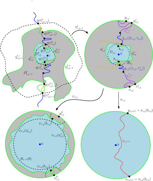
Figure 7.2: Top left: Illustration of two stages of the inductive construction in Section 7.3 (the picture shows a small neighborhood of the point $z\in\mathbf{D}$). Segments of $\eta$ associated with the events $L_{z,j}$ (resp. $\widetilde{E}_{z,j-1}$ and $\widetilde{E}_{z,j}$; the last parts of $E_{z,j-1}$ and $E_{z,j}$) are shown in purple (resp. blue; orange). As in Figure 7.1, balls and curve segments are not shown to scale. Top right: The picture we obtain after applying the map $\pi_{z,j-1}^{\operatorname{f}}:D_{z,j-1}^{\operatorname{f}}\rightarrow\mathbf{D}$. This is the same as the setting of the middle panel in Figure 7.1 with $\eta=\eta_{z,j}$. Note that here $x_{z,j}^{*}\not=x_{z,j}$ and $y_{z,j}^{*}\not=y_{z,j}$ since $\eta_{z,j}$ hits $\partial\mathbf{D}$. Bottom left: The setting we obtain after applying the map $\psi_{z,j}$, which corresponds to the right panel in Figure 7.1. Bottom right: The setting we obtain after applying the map $\pi_{z,j}$. The red curve $\eta_{z,j+1}$ is the image under $\pi_{z,j}$ of the segment of $\eta_{z,j}$ contained in $D_{z,j}$.

7.3.1 Inductive definitions of events

Here we will use the events of Section 7.2 with $\eta$ replaced by a conformal image of an appropriate segment of $\eta$ to define the following objects for $z\in B_{d}(0)$ and $j\in\mathbf{N}$.

• Events $L_{z,j}$, $\widetilde{E}_{z,j}$, $F_{z,j}$, and $E_{z,j}$.

• Points $x_{z,j},y_{z,j},x_{z,j}^{*},y_{z,j}^{*},x_{z,1}^{F},y_{z,1}^{F},b_{z,j}$, and $\overline{b}_{z,j}$.

• Conformal maps $\psi_{z,j}^{L},\phi_{z,j},\psi_{z,j},$ and $\pi_{z,j}$.

• Random times $\sigma_{z,j},\overline{\sigma}_{z,j}$, $\tau_{z,j}$, $\overline{\tau}_{j,z}$, $\tau_{z,1}^{*}$, and $\overline{\tau}_{z,j}^{*}$.

• Curves $\eta_{z,j}$ and $\eta_{z,j}^{\pm}$.

• Fields $h_{z,j}$.

• Domains $D_{z,j}$.

First we consider the case $j=1$. For $z\in B_{d}(0)$, let $f_{z,1}$ be the conformal automorphism of $\mathbf{D}$ satisfying $f_{z,1}(z)=0$ and $f_{z,1}(-i)=-i$. Let $\eta_{z,1}:=f_{z,1}(\eta)$ and let $x_{z,1}:=-i=f_{z,1}(-i)$ and $y_{z,1}:=f_{z,1}(i)$ be its start and end points. Also define the field $h_{z,1}:=h^{\operatorname{f}}\circ f_{z,1}^{-1}-\chi\operatorname{arg}((f_{z,1}^{-1})^{\prime})$, where here $\chi=2/\sqrt{\kappa}-\sqrt{\kappa}/2$ is the imaginary geometry parameter.

Define the event $E_{z,1}$ and the associated objects as in Section 7.2 with $\beta=\beta_{1}$, $u=u_{1}$, $\eta_{z,1}$ in place of $\eta$, and $h_{z,1}$ in place of $h$, and denote these objects with a subscript $z,1$. We recall in particular that $D_{z,1}$ is the domain formed by the auxiliary flow lines $\eta_{z,1}^{\pm}$, with marked points $b_{z,1},\overline{b}_{z,1}\in\partial D_{z,1}$, and we let $\pi_{z,1}:D_{z,1}\rightarrow\mathbf{D}$ be the conformal map with $\pi_{z,1}(0)=0$ and $\pi_{z,1}^{\prime}(0)>0$.

Now suppose $j\geq 2$ and our objects have been defined for all positive integers $l\leq j-1$. If $D_{z,j-1}=\emptyset$, we take all of the objects defined below to be equal to a graveyard point. Otherwise, let $\eta_{z,j}$ be the image under $\pi_{z,j-1}$ of the segment of $\eta_{z,j-1}$ contained in $\overline{D}_{z,j-1}$ (equivalently, the segment of $\eta_{z,j-1}$ from $\eta_{z,j-1}(\tau_{z,j-1})$ to $\overline{\eta}(\overline{\tau}_{z,j-1}$). Then $x_{z,j}=\pi_{z,j-1}(b_{z,j-1})$ and $y_{z,j}=\pi_{z,j-1}(\overline{b}_{z,j-1})$ are the initial and terminal points of $\eta_{z,j}$. Define the field

$$h_{z,j}:=h_{z,j-1}\circ\pi_{z,j-1}^{-1}-\chi\operatorname{arg}(\pi_{z,j-1}^{-1})^{\prime}.$$

Lemma 7.4 implies that $h_{z,j}$ is a GFF with Dirichlet boundary data, $\eta_{z,j}$ is its 0-angle flow line from $-i$ to $y_{z,j}$, and $\eta_{z,j}$ is an SLE${}_{\kappa}(\rho^{1};\rho^{1})$ with force points located on either side of $-i$.

Define the event $E_{z,j}$ and the associated objects as in Section 7.2 with $\beta=\beta_{j}$, $u=u_{j}$, $\eta_{z,j}$ in place of $\eta$, and $h_{z,j}$ in place of $h$ and denote these objects by a subscript $z,j$.

Remark 7.9.

There exists $\widetilde{d}\in(0,1)$, depending only on $d$, such that if $z\in B_{d}(0)$ then each conformal automorphism $\mathbf{D}\rightarrow\mathbf{D}$ taking $z$ to $0$ takes $-i$ and $i$ to a point of $\partial\mathbf{D}$ at distance at least $\widetilde{d}$ from each other, so $|x_{z,1}-y_{z,1}|\geq\widetilde{d}$. By conditions 2 and 3 in the definition of $\widetilde{E}_{z,j}$ and condition 3 in the definition of $F_{z,j}$, after possibly shrinking $\widetilde{d}$ (in a manner depending only on $r$ and $a$) we can arrange that also $|x_{z,j}-y_{z,j}|\geq\widetilde{d}$ for $j\geq 2$.

7.3.2 Objects associated with the full curve $\eta$

Let

$$E_{n}(z):=\bigcap_{j=1}^{n}E_{z,j}.$$ (7.5)

Also define the $\sigma$-algebra

$$\mathcal{F}_{z,n}:=\sigma\left(\eta_{z,j}|_{[0,\tau_{z,j}^{*}]},\,\overline{\eta}_{z,j}|_{[0,\overline{\tau}_{z,j}^{*}]},\eta_{z,j}^{-}|_{[0,t_{z,j}^{-}]},\eta_{z,j}^{+}|_{[0,t_{z,j}^{+}]}\,:\,j\leq n\right)$$ (7.6)

so that $E_{n}(z)\in\mathcal{F}_{z,n}$.

We will also need to define a few additional objects associated with the full curve $\eta$, which are denoted with a superscript ${\operatorname{f}}$ (recall the notational convention described at the beginning of Section 7.1). For $z,j\in\mathbf{N}$, define the conformal map

$$\pi_{z,j}^{\operatorname{f}}:=\pi_{z,j}\circ\dots\circ\pi_{z,1}\circ f_{z,1}.$$ (7.7)

Also set $\pi_{z,0}:=f_{z,1}$. Then $\pi_{z,j}^{\operatorname{f}}:D_{z,j}^{\operatorname{f}}\rightarrow\mathbf{D}$, for $D_{z,j}^{\operatorname{f}}$ a domain in $\mathbf{D}$ containing $z$ and $\pi_{z,j}^{\operatorname{f}}(z)=0$.

For $z\in B_{d}(0)$ and $j\in\mathbf{N}$, let $\tau_{z,j}^{\operatorname{f}}$ and $\tau_{z,j}^{{\operatorname{f}},*}$ (resp. $\overline{\tau}_{z,j}^{{\operatorname{f}},*}$ and $\overline{\tau}_{z,j}^{{\operatorname{f}},*}$) be the times for $\eta$ (resp. $\overline{\eta}$) such that

$$\pi_{z,j-1}^{\operatorname{f}}(\eta(\tau_{z,j}^{\operatorname{f}}))=\eta_{z,j}(\tau_{z,j})\quad\operatorname{and}\quad(\psi_{z,j}\circ\pi_{z,j-1}^{\operatorname{f}})(\eta(\tau_{z,j}^{{\operatorname{f}},*}))=\eta_{z,j}(\tau_{z,j}^{*})$$ (7.8)

(resp. the analogous relation holds for $\overline{\eta}$ and $\overline{\eta}_{z,j}$).

Let $\eta_{z,j}^{{\operatorname{f}},\pm}$ be the flow lines of $h$ with angles $\mp\theta$ started from $\eta(\tau_{z,j})$. Then $\eta_{z,j}^{{\operatorname{f}},\pm}$ trace $\partial D_{z,j}^{\operatorname{f}}$ and if we let $t_{z,j}^{{\operatorname{f}},\pm}$ be the time at which $\eta_{z,j}^{{\operatorname{f}},\pm}$ finishes tracing $\partial D_{z,j}^{\operatorname{f}}$,

$$(\eta_{z,j}^{\pm})^{t_{z,j}^{\pm}}=\pi_{z,j-1}^{\operatorname{f}}((\eta_{z,j}^{{\operatorname{f}},\pm})^{t_{z,j}^{{\operatorname{f}},\pm}}).$$ (7.9)

7.3.3 Choosing of $\beta_{j}$ and $u_{j}$

We now choose the sequences $\beta_{j}\rightarrow\infty$ and $u_{j}\rightarrow 0$ which are used in place of $\beta$ and $u$, respectively, in the definitions of the events in Section 7.2.

By Lemma 7.7 (applied with $\widetilde{d}$ as in Remark 7.9) tells us that for each $u\in(0,1)$, there exists $\beta_{*}(u)=\beta_{*}(u,\widetilde{d})>0$ such that if we are in the setting of Section 7.2 with $\beta\geq\beta_{*}(u)$, either $\rho^{L}=\rho^{R}=\rho^{1}$ or $\rho^{L}=\rho^{R}=0$, and $|x-y|\geq\widetilde{d}$, then

$$C_{u}^{-1}e^{-\beta(\gamma^{*}(q)+\gamma_{0}^{*}(q)u)}\leq\mathbf{P}(E)\leq C_{u}e^{-\beta(\gamma^{*}(q)-\gamma_{0}^{*}(q)u)},$$ (7.10)

where for $u>0$, $C_{u}$ is a constant which is allowed to depend on $u$, $\widetilde{d}$, and the auxiliary parameters but not on $\beta$ or the particular choice of $x$ and $y$. We now choose $\beta_{j}\rightarrow\infty$ and $u_{j}\rightarrow 0$ in such a way that (7.10) remains true with $\beta_{j}$ in place of $\beta$ and $u_{j}$ in place of $u$.

Lemma 7.10.

For each choice of $\widetilde{d}$ (which we recall from Remark 7.9 depends on $d$) and each choice of the auxiliary parameters, there exists $\beta_{0}>0$ such that with $\beta_{j}=\log j+\beta_{0}$, one can choose $(u_{j})_{j\in\mathbf{N}}$ such that the following is true.

1. $u_{j}$ decreases to $0$ as $j\rightarrow\infty$.

2. For each $j\in\mathbf{N}$. we have $\beta_{j}\geq\beta_{*}(u_{j})$ so that (7.10) holds with $\beta_{j}$ in place of $\beta$ and $u_{j}$ in place of $u$.

3. For each $j\in\mathbf{N}$, $C_{u_{j}}\leq e^{\beta_{j}u_{j}\gamma_{0}^{*}(q)}$.

4. $\beta_{j}u_{j}\rightarrow\infty$ as $j\rightarrow\infty$.

Remark 7.11.

The reason we allow $\beta$ and $u$ to vary here is that we eventually want to get a lower bound for the Hausdorff dimension of the sets $\Theta^{s}(D_{\eta})$ and $\widetilde{\Theta}^{s}(D_{\eta})$. If we fixed $u$, we would instead get the Hausdorff dimension of the sets where the limits in the definitions of $\Theta^{s}(D_{\eta})$ and $\widetilde{\Theta}^{s}(D_{\eta})$ are between $s-u$ and $s+u$. In order to allow $u$ to vary, we also need to allow $\beta$ to vary, for otherwise the constants $C_{u}$ in (7.10) would be larger than $e^{\beta}$ when $u$ is very small. The idea in Lemma 7.10 below is to let $u_{j}\rightarrow 0$ and $\beta_{j}\rightarrow\infty$ slowly enough that our estimates are not much different than they would be with fixed $\beta$ and $u$.

Proof of Lemma 7.10.

Fix $u_{0}\in(0,1)$. Choose $\beta_{0}$ much larger than $\Delta\vee\gamma_{0}^{*}(q)^{-1}\log C_{u_{0}}$ and large enough that (7.10) holds with $\beta_{0}$ in place of $\beta$ and $u_{0}$ in place of $u$. Set $\beta_{j}=\log j+\beta_{0}$ for this choice of $\beta_{0}$. We now inductively choose $(u_{j})_{j\in\mathbf{N}}$. Start with a sequence $(u_{l}^{*})_{l\in\mathbf{N}}\subset(0,u_{0})$ which decreases to 0. Let $j_{1}$ be the least positive integer $j$ such that $\beta_{j}\geq\beta_{*}(u_{1}^{*})$, $C_{u_{1}^{*}}\leq e^{\beta_{j}u_{1}^{*}\gamma^{*}_{0}(q)}$, and $\beta_{j}u_{1}^{*}\geq 1$. Such a $j$ exists since $\beta_{j}\rightarrow\infty$ as $j\rightarrow\infty$. Set $u_{j}=u_{0}$ for $j\in\{1,\dots,j_{1}\}$. Inductively, suppose $l\geq 1$ and $j_{1},\ldots,j_{l-1}$ and $u_{j}$ for $j\leq j_{l-1}$ have been defined. Let $j_{l}$ be the least integer $j\geq j_{l-1}+1$ such that $\beta_{j}\geq u_{l}^{*}$, $C_{u_{l}^{*}}\leq e^{\beta_{j}u_{l}^{*}\gamma^{*}_{0}(q)}$, and $\beta_{j}u_{l}^{*}\geq l$. Let $u_{j}=u_{l-1}^{*}$ for $j\in\{j_{l-1}+1,\ldots,j_{l}\}$. It is clear that conditions 2, 3, and 4 hold for this choice of $(u_{j})$. ∎

We henceforth assume that the sequences $(\beta_{j})$ and $(u_{j})$ are chosen as in Lemma 7.10. We also define

$$\overline{\beta}_{m}:=\sum_{j=1}^{m}\beta_{j}\quad\operatorname{and}\quad\overline{u}_{m}:=\sum_{j=1}^{m}\beta_{j}u_{j},\quad\forall m\in\mathbf{N}.$$ (7.11)

Due to our choice of the $\beta_{j}$’s and $u_{j}$’s, we obtain the following estimate for the probabilities of the events $E_{n}(z)$.

Lemma 7.12.

With $E_{n}(z)$ as in (7.5), it holds for each $n\in\mathbf{N}$ that

$$e^{-\overline{\beta}_{n}\gamma^{*}(q)-2\gamma_{0}^{*}(q)\overline{u}_{n}}\preceq\mathbf{P}\left(E_{n}(z)\right)\preceq e^{-\overline{\beta}_{n}\gamma^{*}(q)+2\gamma_{0}^{*}(q)\overline{u}_{n}}$$ (7.12)

with the implicit constants independent of $n$ and uniform for $z\in B_{d}(0)$. The same is true if we replace $(\beta_{j},u_{j})_{j\in\mathbf{N}}$ by $(\beta_{j+m},u_{j+m})_{j\in\mathbf{N}}$ for any $m\in\mathbf{N}$ (both in the definition of $E_{n}(z)$ and in (7.12)), with the implicit constants unchanged.

Proof.

By Lemma 7.4, (7.10), and Remark 7.9, for each $j\in\mathbf{N}$,

$$C_{u_{j}}^{-1}e^{-\beta_{j}(\gamma^{*}(q)+\gamma_{0}^{*}(q)u_{j})}\leq\mathbf{P}(E_{z,j}\,|\,E_{j-1}(z))\leq C_{u_{j}}e^{-\beta_{j}(\gamma^{*}(q)-\gamma_{0}^{*}(q)u_{j})}.$$

The estimate (7.12) follows by multiplying this over all $j\in\{1,\dots,n\}$ and applying condition 3 in Lemma 7.10. ∎

7.4 Analytic properties

In this subsection we study some analytic properties of the events of Section 7.3. The results of this subsection are needed to analyze the correlation structure of our events in the next subsection and to show that the perfect points are in fact contained in the sets whose Hausdorff dimension we want to compute in Section 8. The main result of this subsection is the following proposition.

Lemma 7.13.

Assume we are in the setting of Section 7.3, and recall in particular the event $E_{n}(z)$ for $n\in\mathbf{N}$ and $z\in B_{d}(0)$ from (7.5). On $E_{n}(z)$ let $\Phi^{\operatorname{f}}_{z,n}$ be the conformal map from $\mathbf{D}\setminus(\eta^{\tau_{z,n}^{{\operatorname{f}},*}}\cup\overline{\eta}^{\overline{\tau}_{z,n}^{{\operatorname{f}},*}})$ to $\mathbf{D}$ which takes $-i^{+}$ to $-i$, $i^{-}$ to $i$, and 1 to 1. We can choose the parameter $r$ sufficiently small, in a manner depending only on $a$, and $\beta_{0}$ (and hence every $\beta_{j}$) sufficiently large, in a manner which does not depend on $(u_{j})$ and is uniform for $z\in B_{d}(0)$, in such a way that the following holds a.s. on $E_{n}(z)$, with all implicit constants deterministic and independent of $n$ and uniform for $z\in B_{d}(0)$.

1. We have

   $$e^{-\overline{\beta}_{n}q-2\overline{u}_{n}}\preceq|(\Phi^{\operatorname{f}}_{z,n})^{\prime}(z)|\preceq e^{-\overline{\beta}_{n}q+2\overline{u}_{n}}.$$

2. There is a constant $\lambda_{*}>0$, independent of $n$ and uniform for $z\in B_{d}(0)$, such that

   $$e^{-\overline{\beta}_{n}-\lambda_{*}n}\leq\operatorname{dist}\left(z,\eta^{\tau_{z,n}^{{\operatorname{f}},*}}\cup\overline{\eta}^{\overline{\tau}_{z,n}^{{\operatorname{f}},*}}\right)\leq e^{-\overline{\beta}_{n}+\lambda_{*}n}.$$

3. We have

   $$|\eta(\tau_{z,n}^{{\operatorname{f}},*})-z|\asymp|\overline{\eta}(\overline{\tau}_{z,n}^{{\operatorname{f}},*})-z|\asymp\operatorname{dist}\left(z,\eta^{\tau_{z,n}^{{\operatorname{f}},*}}\cup\overline{\eta}^{\overline{\tau}_{z,n}^{{\operatorname{f}},*}}\right)$$

4. We have

   $$e^{-\overline{\beta}_{n}-\lambda_{*}n}\leq\operatorname{dist}(z,\partial D_{z,n}^{\operatorname{f}})\leq\operatorname{diam}D_{z,n}^{\operatorname{f}}\leq e^{-\overline{\beta}_{n}+\lambda_{*}n}.$$

Lemma 7.13 is the only statement from this subsection which will be needed in later sections, and the proof is a rather technical complex analysis argument. The reader may wish to skip the rest of this subsection to see the more probabilistic aspects of the proofs of our main results.

It may seem at first glance that Lemma 7.13 should be a simple consequence of the definitions in Section 7.3 and the chain rule. This is not the case, however, as at each stage in our construction we restrict to the domain $D_{z,j}$ so $\Phi_{z,n}^{\operatorname{f}}$ (which is defined on all of $\mathbf{D}\setminus(\eta^{\tau_{z,n}^{{\operatorname{f}},*}}\cup\overline{\eta}^{\overline{\tau}_{z,n}^{{\operatorname{f}},*}})$) cannot be expressed as a composition of maps defined in Section 7.3. To prove the lemma, we will express $\Phi_{z,n}^{\operatorname{f}}$ as a composition of maps corresponding to scales $j=1,\dots,n$ (see in particular (7.14)) then argue that these maps are in some sense comparable to the maps appearing in Section 7.3.

To prove Lemma 7.13 we will need to compare the derivatives of several different maps. To this end, we will define the following objects.

• Conformal maps $\psi^{\operatorname{f}}_{z,j}$, $\widetilde{\phi}_{z,j}$, $\widehat{\phi}_{z,j}$, $f_{z,j}$, and $g_{z,j}$.

• Random times $\widetilde{\tau}_{z,j}^{*}$ and $\overline{\widetilde{\tau}}_{z,j}^{*}$.

• Points $\widetilde{x}_{z,j}$ and $\widetilde{y}_{z,j}$.

• Curves $\widetilde{\eta}_{z,j}$.

For the definitions, we recall the notational conventions discussed at the beginning of Section 7.1. We assume we are working on the event $E_{j}(z)$ for all of these definitions.

For $j\in\mathbf{N}$, let $\psi^{\operatorname{f}}_{z,j}$ be the conformal map from $\mathbf{D}\setminus(\eta^{\tau_{z,j}^{{\operatorname{f}},*}}\cup\overline{\eta}^{\overline{\tau}_{z,j}^{{\operatorname{f}},*}})$ to $\mathbf{D}$ which fixes $0$ and whose derivative at $0$ has the same argument as $(\Phi^{\operatorname{f}}_{z,j})^{\prime}(z)$ (the latter map is defined in Lemma 7.13).

For $j=1$, the conformal automorphism $f_{z,1}$ taking $z$ to $0$ has already been defined in Section 7.2. For $j\geq 2$, we let $f_{z,j}:\mathbf{D}\rightarrow\mathbf{D}$ be the conformal automorphism which takes $\Phi^{\operatorname{f}}_{z,j-1}(z)$ to $0$ with $f_{z,j}^{\prime}(\Phi^{\operatorname{f}}_{z,j-1}(z))>0$. Observe that $\psi_{z,j-1}^{\operatorname{f}}=f_{z,j}\circ\Phi^{\operatorname{f}}_{z,j-1}$ (here we take $\Phi^{\operatorname{f}}_{z,0}$ to be the identity map and $\psi_{z,0}^{\operatorname{f}}=f_{z,1}$ in the case $j=1$).

For $j\geq 1$, let $\widetilde{\eta}_{z,j}$ be the image under $\psi_{z,j-1}^{\operatorname{f}}$ of the part of $\eta$ between $\eta(\tau_{z,j-1}^{{\operatorname{f}},*})$ and $\overline{\eta}(\overline{\tau}_{z,j-1}^{{\operatorname{f}},*})$. Note that $\widetilde{\eta}_{z,j}$ is a conformal image of the same part of the curve $\eta$ as $\eta_{z,j}$, but the conformal map used to get $\widetilde{\eta}_{z,j}$ is defined on $\mathbf{D}\setminus(\eta^{\tau_{z,j}^{{\operatorname{f}},*}}\cup\overline{\eta}^{\overline{\tau}_{z,j}^{{\operatorname{f}},*}})$ rather than the pocket $D_{z,j}^{\operatorname{f}}$. Let $\widetilde{\tau}_{z,j}^{*}$ and $\overline{\widetilde{\tau}}_{z,j}^{*}$ be the times for $\widetilde{\eta}_{z,j}$ and its time reversal $\overline{\widetilde{\eta}}_{z,j}$ such that

$$\psi_{z,j}^{\operatorname{f}}(\eta(\tau_{z,j}^{{\operatorname{f}},*}))=\widetilde{\eta}_{z,j}(\widetilde{\tau}_{z,j}^{*})\quad\operatorname{and}\quad\psi_{z,j}^{\operatorname{f}}(\overline{\eta}(\overline{\tau}_{z,j}^{{\operatorname{f}},*}))=\overline{\widetilde{\eta}}_{z,j}(\overline{\widetilde{\tau}}_{z,j}^{*})$$

Let $\widetilde{x}_{z,j}$ and $\widetilde{y}_{z,j}$ be the start and end points for $\widetilde{\eta}_{z,j}$. Let $\widetilde{\phi}_{z,j}:\mathbf{D}\setminus(\widetilde{\eta}_{z,j}^{\widetilde{\tau}_{z,j}^{*}}\cup\overline{\widetilde{\eta}}_{z,j}^{\overline{\widetilde{\tau}}_{z,j}})\rightarrow\mathbf{D}$ which takes $\widetilde{x}_{z,j}^{+}$ to $-i$, $\widetilde{y}_{z,j}^{-}$ to $i$ and the midpoint of $[\widetilde{x}_{z,j},\widetilde{y}_{z,j}]_{\partial\mathbf{D}}$ to 1. Let $g_{z,j}:\mathbf{D}\rightarrow\mathbf{D}$ be the conformal automorphism taking $(\widetilde{\phi}_{z,j}\circ f_{z,j})(b)$ to $b$ for $b=-i^{+},i^{-},1$. Let

$$\widehat{\phi}_{z,j}:=g_{z,j}\circ\widetilde{\phi}_{z,j}\circ f_{z,j}:\mathbf{D}\setminus(\widetilde{\eta}_{z,j}^{\widetilde{\tau}_{z,j}^{*}}\cup\overline{\widetilde{\eta}}_{z,j}^{\overline{\widetilde{\tau}}_{z,j}})\rightarrow\mathbf{D}$$ (7.13)

and observe that that (with $\Phi^{\operatorname{f}}_{z,j}$ as in Lemma 7.13)

$$\Phi^{\operatorname{f}}_{z,j}=\widehat{\phi}_{z,j}\circ\cdots\circ\widehat{\phi}_{z,1}.$$ (7.14)

See Figure 7.3 for an illustration of these maps in the case $j=2$ (which has all of the features of the general case).

The following straightforward lemma tells us that on $E_{n}(z)$, the derivatives at $0$ of the conformal maps from $D_{z,n}^{\operatorname{f}}$ to $\mathbf{D}$ and from $\mathbf{D}\setminus(\eta_{z,n}^{\tau_{z,n}^{{\operatorname{f}},*}}\cup\overline{\eta}_{z,n}^{\overline{\tau}_{z,n}^{{\operatorname{f}},*}})$ to $\mathbf{D}$ which take $z$ to $0$ are comparable (equivalently, by the Koebe quarter theorem, the distance from $z$ to $\partial D_{z,n}^{\operatorname{f}}$ is comparable to the distance from $z$ to $\eta_{z,n}^{\tau_{z,n}^{{\operatorname{f}},*}}\cup\overline{\eta}_{z,n}^{\overline{\tau}_{z,n}^{{\operatorname{f}},*}}$).

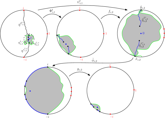
Figure 7.3: An illustration of some of the maps associated with the events $E_{z,1}$ and $E_{z,2}$. The images of $-i$, $i$, and 1 are shown in red. The images of $z$ are shown in blue. The black curves are associated with the event $E_{z,1}$ and the blue curves are associated with the event $E_{z,2}$. The map $\widehat{\phi}_{z,2}$ is the composition of the last three maps in the figure. The map $\Phi^{\operatorname{f}}_{z,2}$ is the composition of all four maps.

Lemma 7.14.

If $\beta_{0}$ is chosen sufficiently large, independently of everything else, then on the event $E_{n}(z)$,

$$|(\pi_{z,n}^{\operatorname{f}})^{\prime}(z)|\asymp|(\psi_{z,n}^{\operatorname{f}})^{\prime}(z)|,$$ (7.15)

with the implicit constants independent of $n$ and uniform for $z\in B_{d}(0)$.

Proof.

Assume we are working on the event $E_{n}(z)$. Let $\widehat{\pi}_{z,n-1}$ be the conformal map from $\psi_{z,n}^{\operatorname{f}}(D_{z,n-1}^{\operatorname{f}})$ to $\mathbf{D}$ with $\widehat{\pi}_{z,n-1}(0)=0$ and $\widehat{\pi}_{z,n-1}^{\prime}(0)>0$ (in the case $n=1$, we take $\widehat{\pi}_{z,n-1}$ to be the identity). Let $\widehat{\pi}_{z,n}^{*}$ be the conformal map from $(\widehat{\pi}_{z,n-1}\circ\psi_{z,n}^{\operatorname{f}})(D^{\operatorname{f}}_{z,n})$ to $\mathbf{D}$ with $\widehat{\pi}_{z,n}^{*}(0)=0$ and $\operatorname{arg}(\widehat{\pi}_{z,n}^{*})^{\prime}(0)$ chosen in such a way that

$$\pi_{z,n}^{\operatorname{f}}=\widehat{\pi}_{z,n}^{*}\circ\widehat{\pi}_{z,n-1}\circ\psi_{z,n}^{\operatorname{f}}.$$ (7.16)

By the Beurling estimate and [Law05, Exercise 2.7] the diameters of the connected components of $\mathbf{D}\setminus\psi_{z,n}^{\operatorname{f}}(D_{z,n-1}^{\operatorname{f}})$ each tend uniformly to $0$ as $\beta_{n}\rightarrow\infty$ (and hence also as $\beta_{0}\rightarrow\infty$). Therefore, if $\beta_{0}$ is chosen sufficiently large, then $|(\widehat{\pi}_{z,n-1})^{\prime}(0)|\asymp 1$.

Let $\psi_{z,n}:\mathbf{D}\setminus(\eta_{z,n}^{\tau_{z,n}}\cup\overline{\eta}_{z,n}^{\overline{\tau}_{z,n}})\rightarrow\mathbf{D}$ be as in condition 2 in the definition of $F_{z,n}$. The set $(\widehat{\pi}_{z,n-1}\circ\psi_{z,n}^{\operatorname{f}})(\partial D_{z,n}^{\operatorname{f}})$ is the image of $\psi_{z,n}(\partial D_{z,n})$ under a conformal map which fixes $0$ and maps the complement of the set $\psi_{z,n}(\eta_{z,1}([\tau_{z,n},\tau_{z,n}^{*}]))\cup\psi_{z,n}(\overline{\eta}_{z,n}([\overline{\tau}_{z,n},\overline{\tau}_{z,n}^{*}])$ to $\mathbf{D}$. By condition 2 in the definition of $E_{z,n}$, the distance from $0$ to $(\widehat{\pi}_{z,n-1}\circ\psi_{z,n}^{\operatorname{f}})(\partial D_{z,n}^{\operatorname{f}})$ is proportional to the distance from $0$ to $\psi_{z,n}(\partial D_{z,n})$. By condition 1 in the definition of $F_{z,n}$, this distance is $\asymp 1$. Consequently, $|(\widehat{\pi}_{z,n}^{*})^{\prime}(0)|\asymp 1$ so (7.15) follows from (7.16). ∎

Lemma 7.15.

Let $\zeta\in(0,a/100)$. If the auxiliary parameter $r$ is at most some constant depending only on $a$ and $\zeta$, and $\beta_{0}$ is chosen sufficiently large (in a manner which does not depend on $(u_{j})$ and is uniform for $z\in B_{d}(0)$) then for any $n\in\mathbf{N}$ and any sub-arc $I$ of $[\widetilde{x}_{z,n+1},\widetilde{y}_{z,n+1}]_{\partial\mathbf{D}}$ lying at distance at least $\zeta$ from $\widetilde{x}_{z,n+1}$ and $\widetilde{y}_{z,n+1}$, the map $\widetilde{\phi}_{z,n+1}$ is Lipschitz on $I$ and $\widetilde{\phi}_{z,n+1}^{-1}$ is Lipschitz on $\widetilde{\phi}_{z,n+1}(I)$ on the event $E_{n}(z)$ with Lipschitz constants independent of $(\beta_{j})$ and $(u_{j})$ and uniform for $z\in B_{d}(0)$ and $n\in\mathbf{N}$.

Proof.

See Figure 7.4 for an illustration of the argument. Throughout, we work on the event $E_{n}(z)$.

Let $A:=\psi_{z,n}^{\operatorname{f}}((\eta_{z,n}^{{\operatorname{f}},+})^{t_{z,n}^{+}})$, where here we recall that $\eta_{z,n}^{{\operatorname{f}},+}$ is the stage-$n$ right auxiliary flow line for $h$. Then $A$ disconnects $\widetilde{\eta}_{z,n+1}$ from $I$ in $\partial\mathbf{D}$. We claim that if $r$ is chosen sufficiently small then there is a constant $\delta>0$, depending only on $\zeta$, $d$, and the auxiliary parameters from Definition 7.1, such that for large enough $\beta_{0}$,

$$E_{n}(z)\subset\{\operatorname{dist}(A,I)\geq\delta\}.$$ (7.17)

Given the claim, the statement of the lemma follows from Lemma 2.8 and the fact that $\widetilde{\eta}_{z,n+1}$ lies to the left of $A$ due to the monotonicity of flow lines [MS16c, Theorem 1.5].

Let $\psi_{z,n}^{*}$ be a conformal map from the connected component of $\mathbf{D}\setminus(\eta_{z,n}^{\tau_{z,n}^{*}}\cup\overline{\eta}_{z,n}^{\overline{\tau}_{z,n}^{*}})$ containing 1 on it boundary to $\mathbf{D}$ which fixes 0. This map is defined only up to a rotation, which we will specify shortly. Let $\eta_{z,n+1}^{*}$ be the image under $\psi_{z,n}^{*}$ of the part of $\eta_{z,n}$ between $\eta_{z,n}(\tau_{z,n}^{*})$ and $\overline{\eta}_{z,n}(\overline{\tau}_{z,n}^{*})$. We can choose the normalization for $\psi_{z,n}^{*}$ in such a way that

$$\eta_{z,n+1}^{*}=\widehat{\pi}_{z,n-1}(\widetilde{\eta}_{z,n+1}),$$

with $\widehat{\pi}_{z,n-1}$ as in the proof of Lemma 7.14.

By condition 3 in the definition of $\widetilde{E}_{z,n}$ and condition 2 in the definition of $E_{z,n}$, the set $\mathbf{D}\setminus\psi_{z,n}^{\operatorname{f}}(D_{z,n-1}^{\operatorname{f}})$ lies at distance at least a positive constant depending only on $a$ from $\widetilde{x}_{z,n}$ and $\widetilde{y}_{z,n}$ on $E_{n}(z)$. Since the diameters of the connected components of $\mathbf{D}\setminus\psi_{z,n}^{\operatorname{f}}(D_{z,n-1}^{\operatorname{f}})$ and $\partial\mathbf{D}$ each tend to $0$ uniformly as $\beta_{n}\rightarrow\infty$ (by the argument of Lemma 7.14), the map $\widehat{\pi}_{z,n-1}^{-1}$ is nearly constant near $\widetilde{x}_{z,n}$ and $\widetilde{y}_{z,n}$ if $\beta_{0}$ (and hence also $\beta_{n}$) is sufficiently large. By the Schwarz lemma $\widehat{\pi}_{z,n-1}^{-1}$ increases distances to $\partial\mathbf{D}$. Hence the distance from $A$ to $I$ is at least an $n$-independent constant times the distance from $\widehat{A}$ to $I$ if $\beta_{n}$ is chosen sufficiently large, where $\widehat{A}:=\widehat{\pi}_{z,n-1}(A)$. Hence it is enough to prove (7.17) with $\widehat{A}$ in place of $A$.

Let $I^{\prime}\supset I$ be a slightly larger arc. By condition 3 in the definition of $\widetilde{E}_{z,n}$, condition 2 in the definition of $E_{z,n}$, and a harmonic measure estimate, the distance from $\widehat{A}$ to $I$ is $\succeq$ the distance from $\psi_{z,n}((\eta_{z,n}^{+})^{t_{z,n}^{+}})$ to $I^{\prime}$ if $r$ is chosen sufficiently small, depending only on $a$ and $\zeta$, where $\psi_{z,n}$ is as in the definition of $F_{z,n}$. We conclude by applying condition 4 in the definition of $F_{z,n}$. ∎

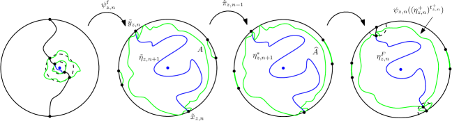
Figure 7.4: An illustration of the maps used in the proof of Lemma 7.15. In order to control the distance from $\widetilde{\eta}_{z,n+1}$ to an arc on the right boundary of the disk, we compare $\widetilde{\eta}_{z,n+1}$ to the curve $\eta_{z,n+1}^{*}$ and then to the curve $\eta_{z,n}^{F}$ which is the image under $\psi_{z,n}$ of the part of $\eta_{z,n}$ between $\eta_{z,n}(\tau_{z,n})$ and $\overline{\eta}_{z,n}(\overline{\tau}_{z,n})$. The distance from the last curve to an appropriate arc of the right boundary is bounded below by condition 4 in the definition of $F_{z,n}$.

We can now get an estimate for the derivatives of our $\phi$-type conformal maps (which, recall, are specified by the images of three boundary points). Iterating this estimate will eventually lead to Lemma 7.13.

Lemma 7.16.

If the auxiliary parameter $r$ in the definition of $E_{z,n}$ is at most some universal constant, then on $E_{n}(z)$,

$$e^{-\beta_{n}(q+u_{n})}\preceq|\phi^{\prime}(w)|\preceq e^{-\beta_{n}(q-u_{n})}$$ (7.18)

where the pair $(\phi,w)$ is any one of $(\phi_{z,n},0),(\widetilde{\phi}_{z,n},0)$, or $(\widehat{\phi}_{z,n},\Phi^{\operatorname{f}}_{z,n-1}(z))$. The implicit constants are independent of $n$ and uniform for $z\in B_{d}(0)$.

Proof.

By condition 2 in the definition of $\widetilde{E}_{z,n}$, the statement of the lemma is true for $(\phi,w)=(\phi_{z,n},0)$. We will now transfer the estimate (7.18) from $\phi_{z,n}$ to $\widetilde{\phi}_{z,n}$ to $\widehat{\phi}_{z,n}$. This latter map is our primary interest, mostly because of (7.14). Throughout, we assume that $E_{n}(z)$ occurs and require all implicit constants to be independent of $n$ and uniform for $z\in B_{d}(0)$.

Let $\phi_{z,n}^{*}$ be the conformal map from the connected component of $\mathbf{D}\setminus(\eta_{z,n}^{\tau_{z,n}^{*}}\cup\overline{\eta}_{z,n}^{\overline{\tau}_{z,n}^{*}})$ containing $0$ to $\mathbf{D}$ which takes $(x^{*}_{z,n})^{+}$ to $-i$, $(y_{z,n}^{*})^{-}$ to $i$, and the midpoint of $[x_{z,n}^{*},y_{z,n}^{*}]_{\partial\mathbf{D}}$ to 1. Intuitively, $\phi_{z,n}^{*}$ is a slight perturbation of $\phi_{z,n}$ (which is defined in the same manner but with $\tau_{z,n}$ and $\overline{\tau}_{z,n}$ in place of $\tau_{z,n}^{*}$ and $\overline{\tau}_{z,n}^{*}$). It is easily seen from condition 2 in the definition of $E_{z,n}$ that (7.18) for $(\phi_{z,n},0)$ implies (7.18) for $(\phi_{z,n}^{*},0)$.

To transfer from $\phi_{z,n}^{*}$ to $\widetilde{\phi}_{z,n}$, we apply Lemma B.1 to find that for any arc $I\subset[x_{z,n}^{*},y_{z,n}^{*}]_{\partial\mathbf{D}}$ with length $\asymp 1$,

$$|\widetilde{\phi}_{z,n}^{\prime}(0)|\asymp\operatorname{dist}\left(0,\widetilde{\eta}_{z,n}^{\widetilde{\tau}_{z,n}^{*}}\cup\overline{\widetilde{\eta}}_{z,n}^{\overline{\widetilde{\tau}}_{z,n}^{*}}\right)^{-1}\operatorname{hm}^{0}\left([\widetilde{x}_{z,n},\widetilde{y}_{z,n}]_{\partial\mathbf{D}};\mathbf{D}\setminus(\widetilde{\eta}_{z,n}^{\widetilde{\tau}_{z,n}^{*}}\cup\overline{\widetilde{\eta}}_{z,n}^{\overline{\widetilde{\tau}}_{z,n}^{*}})\right)\quad\operatorname{and}$$

$$\qquad|(\phi_{z,n}^{*})^{\prime}(0)|\asymp\operatorname{dist}\left(0,\eta_{z,n}^{\tau_{z,n}^{*}}\cup\overline{\eta}_{z,n}^{\overline{\tau}_{z,n}^{*}}\right)^{-1}\operatorname{hm}^{0}\left(I;\mathbf{D}\setminus(\eta_{z,n}^{\tau_{z,n}^{*}}\cup\overline{\eta}_{z,n}^{\overline{\tau}_{z,n}^{*}})\right)$$ (7.19)

By Lemma 7.14 (applied with $n-1$ in place of $n$) and the Koebe quarter theorem,

$$\operatorname{dist}\left(0,\widetilde{\eta}_{z,n}^{\widetilde{\tau}_{z,n}^{*}}\cup\overline{\widetilde{\eta}}_{z,n}^{\overline{\widetilde{\tau}}_{z,n}^{*}}\right)\asymp\operatorname{dist}\left(0,(\eta_{z,n}^{\tau_{z,n}^{*}}\cup\overline{\eta}_{z,n}^{\overline{\tau}_{z,n}^{*}}\right)$$ (7.20)

with the implicit constant independent of $n$ and uniform for $z\in B_{d}(0)$. Moreover, it is easily seen from condition 3 in the definition of $F_{z,n-1}$ that the harmonic measure terms in (7.4) are likewise proportional (here we recall that $[x_{z,n}^{*},y_{z,n}^{*}]_{\partial\mathbf{D}}=\pi_{z,n-1}^{\operatorname{f}}(\eta_{z,n-1}^{{\operatorname{f}},+}\cap D_{z,n-1}^{\operatorname{f}})$). Thus we obtain (7.18) for $\widetilde{\phi}_{z,n}$ from (7.18) for $\phi_{z,n}^{*}$.

To transfer the estimate to $\widehat{\phi}_{z,n}$, recall (7.13) and write

$$|\widehat{\phi}_{z,n}^{\prime}(\Phi^{\operatorname{f}}_{z,n-1}(z))|=|g_{z,n}^{\prime}(\widetilde{\phi}_{z,n}(0))||\widetilde{\phi}_{z,n}^{\prime}(0)||f_{z,n}^{\prime}(\Phi^{\operatorname{f}}_{z,n-1}(z))|,$$ (7.21)

where here we take $\Phi^{\operatorname{f}}_{z,0}$ to be the identity map in the case $n=0$. By condition 3 in the definition of $\widetilde{E}_{n-1}$, we can find $\zeta>0$ depending only on $a$ such that $f_{z,n}([-i,i]_{\partial\mathbf{D}})$ lies at distance at least $\zeta$ from $\widetilde{x}_{z,n}$ and $\widetilde{y}_{z,n}$ on $E_{n-1}(z)$. By Lemma 7.15, on $E_{n-1}(z)$, it holds that $\widetilde{\phi}_{z,n}$ distorts the distances between points in $f_{z,n}([-i,i]_{\partial\mathbf{D}})$ by at most a constant factor (here we use that $z\in B_{d}(0)$ in the case $n=1$). The maps $g_{z,n}$ and $f_{z,n}^{-1}$ are two conformal automorphisms of $\mathbf{D}$ and each takes three points in $[-i,i]_{\partial\mathbf{D}}$ (which lie at uniformly positive distance from $\pm i$) to $-i$, $i$, and 1. Since the distances amongst the marked points for these two conformal maps differ by a constant factor, it follows easily that

$$|g_{z,n}^{\prime}(w_{1})|\asymp|(f_{z,n}^{-1})^{\prime}(w_{2})|$$

for any points $w_{1}$ and $w_{2}$ in the left half of $\mathbf{D}$. By combining this with (7.21) and the estimate (7.18) for $\widetilde{\phi}_{z,n}$, we conclude. ∎

Proof of Lemma 7.13.

Throughout, we require all implicit constants to be independent of $n$ and uniform for $z\in B_{d}(0)$. Assume $E_{n}(z)$ occurs and that $r$ and $\beta_{0}$ have been chosen so that the conclusion of Lemma 7.16 holds. Assertion 1 is immediate from Lemma 7.16 and the relation (7.14). Note that we can absorb the implicit constants in (7.18) into an additional factor of $e^{\overline{u}_{n}}$ due to condition 4 of Lemma 7.10.

To prove assertion 2, we induct on $n$. The case $n=1$ is immediate from the definitions of the events. Now suppose $n\geq 2$ and assertion 2 has been proven with $n$ replaced by $n-1$. Since $(\psi_{z,n-1}^{\operatorname{f}})^{-1}$ maps $\mathbf{D}\setminus(\widetilde{\eta}_{z,n}^{\widetilde{\tau}_{z,n}^{*}}\cup\overline{\widetilde{\eta}}_{z,n}^{\overline{\widetilde{\tau}}_{z,n}^{*}})$ to $\mathbf{D}\setminus(\eta^{\tau_{z,n}^{{\operatorname{f}},*}}\cup\overline{\eta}^{\overline{\tau}_{z,n}^{{\operatorname{f}},*}})$ and fixes 0, the Koebe quarter theorem implies that

$$\operatorname{dist}\left(z,\eta^{\tau_{z,n}^{{\operatorname{f}},*}}\cup\overline{\eta}^{\overline{\tau}_{z,n}^{{\operatorname{f}},*}}\right)\asymp|((\psi_{z,n-1}^{\operatorname{f}})^{-1})^{\prime}(0)|\operatorname{dist}\left(0,\widetilde{\eta}_{z,n}^{\widetilde{\tau}_{z,n}^{*}}\cup\overline{\widetilde{\eta}}_{z,n}^{\overline{\widetilde{\tau}}_{z,n}^{*}}\right).$$ (7.22)

By a second application of the Koebe quarter theorem,

$$|((\psi_{z,n-1}^{\operatorname{f}})^{-1})^{\prime}(0)|\asymp\operatorname{dist}\left(z,\eta^{\tau_{z,n-1}^{{\operatorname{f}},*}}\cup\overline{\eta}^{\overline{\tau}_{z,n-1}^{{\operatorname{f}},*}}\right).$$ (7.23)

By the inductive hypothesis,

$$e^{-\overline{\beta}_{n-1}-\lambda_{*}(n-1)}\preceq\operatorname{dist}\left(z,\eta^{\tau_{z,n-1}^{{\operatorname{f}},*}}\cup\overline{\eta}^{\overline{\tau}_{z,n-1}^{{\operatorname{f}},*}}\right)\preceq e^{-\overline{\beta}_{n-1}+\lambda_{*}(n-1)}.$$ (7.24)

By (7.20) and the definition of $E_{z,n}$,

$$\operatorname{dist}\left(0,\widetilde{\eta}_{z,n}^{\widetilde{\tau}_{z,n}^{*}}\cup\overline{\widetilde{\eta}}_{z,n}^{\overline{\widetilde{\tau}}_{z,n}^{*}}\right)\asymp e^{-\beta_{n}}$$ (7.25)

on $E_{n}(z)$. Provided $\lambda_{*}$ is chosen sufficiently large, independently of $n$ and $z\in B_{d}(0)$, we can now complete the induction by combining (7.22), (7.23), (7.24), and (7.25).

By condition 3 in the definition of $\widetilde{E}_{z,n}$ and condition 2 in the definition of $E_{z,n}$, if we choose $r$ sufficiently small relative to $a$ then the harmonic measure from $z$ of each of the two sides of $\eta^{\tau_{z,n}^{{\operatorname{f}},*}}$ (resp. each of the two sides of $\overline{\eta}^{\overline{\tau}_{z,n}^{{\operatorname{f}},*}}$) in $\mathbf{D}\setminus(\eta^{\tau_{z,n}^{{\operatorname{f}},*}}\cup\overline{\eta}^{\overline{\tau}_{z,n}^{{\operatorname{f}},*}})$ is at least some constant which does not depend on $n$ or the particular choice of $z\in B_{d}(0)$. By the Beurling estimate this implies assertion 3.

For assertion 4, we use assertion 2 (with $n-1$ in place of $n$) and the Koebe quarter theorem to see that there exists radii $\rho^{\prime}>\rho>$0 such that $\rho\succeq e^{-\overline{\beta}_{n}-\lambda_{*}n}$, $\rho^{\prime}\preceq e^{-\overline{\beta}_{n}+\lambda_{*}n}$, $(\psi_{z,n-1}^{\operatorname{f}})^{-1}(\mathcal{B}_{\beta_{n}+\Delta})\supset B_{\rho}(z)$, and $(\psi_{z,n-1}^{\operatorname{f}})^{-1}(\mathcal{B}_{\beta_{n}-\Delta})\subset B_{\rho^{\prime}}(z)$. By combining this with condition 1 in the definition of $F_{z,n}$ we see that assertion 4 holds (after possibly increasing $\lambda_{*}$). ∎

7.5 Probabilistic properties

Continue to assume we are in the setting of Section 7.3. In this subsection we will prove estimates for the correlations of the events $E_{n}(z)$ of (7.5). These estimates will eventually lead to our two-point estimate, which we now state.

Proposition 7.17.

Let $z,w\in B_{d}(0)$. Let $\lambda_{*}$ be the constant from Lemma 7.13 and for $n\in\mathbf{N}$, defined the events $E_{n}(z)$ and $E_{n}(w)$ as in (7.5). Choose $k\in\mathbf{N}$ such that $e^{-\overline{\beta}_{k+1}-\lambda_{*}(k+1)}\leq|z-w|\leq e^{-\overline{\beta}_{k}-\lambda_{*}k}$. We can choose the auxiliary parameters in a manner depending only on $d$ such that the following is true. If $\beta_{0}$ is chosen sufficiently large (depending on the auxiliary parameters), then for any $n\in\mathbf{N}$ with $\overline{\beta}_{n}-\lambda_{*}n\geq\overline{\beta}_{k+1}+\lambda_{*}(k+2)$,

$$\mathbf{P}(E_{n}(z)\cap E_{n}(w))\preceq e^{\overline{\beta}_{k}o_{k}(1)}\frac{\mathbf{P}(E_{n}(z))\mathbf{P}(E_{n}(w))}{\mathbf{P}(E_{k}(w))}$$ (7.26)

with the implicit constants independent of $n$ and $k$, the $o_{k}(1)$ independent of $n$, and both uniform for $z,w\in B_{d}(0)$.

Remark 7.18.

In the setting of Proposition 7.17, $e^{-\overline{\beta}_{k}}=|z-w|^{1+o_{|z-w|}(1)}$ so by Lemma 7.12 we can rewrite the estimate (7.26) as

$$\mathbf{P}(E_{n}(z)\cap E_{n}(w))\preceq|z-w|^{-\gamma^{*}(q)+o_{|z-w|}(1)}\mathbf{P}(E_{n}(z))\mathbf{P}(E_{n}(w)).$$ (7.27)

This is the form of the estimate we will use when we prove lower bounds for the Hausdorff dimensions of our sets. We emphasize that there is no $e^{-\overline{\beta}_{n}o_{n}(1)}$ error in (7.27); this is important for the proofs in Section 8.

Throughout this subsection, we fix the auxiliary parameters from Definition 7.1 in such a way that the conclusions of Lemmas 7.7 and 7.13 hold. The starting point of the proof of Proposition 7.17 is the following absolute continuity statement. Note that to get strict mutual absolute continuity, we need to skip one scale (i.e., we condition on what happens up to stage $n-2$ and look at the objects at or after stage $n$) in order to re-randomize the locations of the endpoints of the curve.

Lemma 7.19.

Suppose we are in the setting of Section 7.3 and for $z\in B_{d}(0)$ and $j\in\mathbf{N}$, let $H_{z,j}$ be the event of Lemma 7.8 with $\eta=\eta_{z,j}$ and $r_{H}$ chosen sufficiently small that $E_{z,j}\subset H_{z,j}$. If $\beta_{0}$ is chosen sufficiently large, independently of $z\in B_{d}(0)$, then for $n\geq 2$ and $z\in B_{d}(0)$, the following two laws are a.s. strictly mutually absolutely continuous (s.m.a.c.; Definition C.1) modulo rotations of $\mathbf{D}$, with deterministic implicit constants uniform in $n$, $(\beta_{j},u_{j})_{j\geq 1}$, and $z\in B_{d}(0)$.

1. The conditional joint law of $\eta_{z,n}$ and $\left\{(\eta_{z,j}^{+},\eta_{z,j}^{-})\right\}_{j\geq n}$ given the event $H_{z,n-1}$ and the $\sigma$-algebra $\mathcal{F}_{z,n-2}$ of (7.6) on the event $E_{n-2}(z)$.

2. The conditional joint law of $\eta_{z,2}$ and $\left\{(\eta_{z,2}^{+},\eta_{z,2}^{-})\right\}_{j\geq 1}$ given $H_{z,1}$ with the sequence $(\beta_{j},u_{j})_{j\in\mathbf{N}}$ replaced by $(\beta_{n+j-2},u_{n+j-2})_{j\in\mathbf{N}}$.

Proof.

The $\sigma$-algebra $\mathcal{F}_{z,n}$ for $n\in\mathbf{N}$ is generated by flow lines of $h$ which lie outside of $D_{z,n}^{\operatorname{f}}$, so since $h$ determines its flow lines in a local manner (this follows from [MS16c, Theorem 1.2] and the fact that flow lines are local sets in the sense of [SS13]) we infer that $\mathcal{F}_{z,n}\subset\sigma(D_{z,n}^{\operatorname{f}},h|_{\mathbf{D}\setminus D})$.

By Lemma 7.4 and induction, we infer that for $n\geq 1$ and any $\mathfrak{x},\mathfrak{y}\in\partial\mathbf{D}$, the conditional joint law of $\eta_{z,n}$ and $\left\{(\eta_{z,j}^{+},\eta_{z,j}^{-})\right\}_{j\geq n}$ given $\mathcal{F}_{z,n-1}$ on the event that the start and end points $x_{z,n}$ and $y_{z,n}$ for $\eta_{z,n}$ are equal to $\mathfrak{x}$ and $\mathfrak{y}$, respectively, coincides with the conditional joint law of $\eta_{z,2}$ and $\left\{(\eta_{z,2}^{+},\eta_{z,2}^{-})\right\}_{j\geq 1}$ given $\{x_{z,2}=\mathfrak{x},y_{z,2}=\mathfrak{y}\}$ with the sequence $(\beta_{j},u_{j})_{j\in\mathbf{N}}$ replaced by $(\beta_{n+j-2},u_{n+j-2})_{j\in\mathbf{N}}$.

Since we require only strict mutual absolute continuity modulo rotations of $\mathbf{D}$, in order to prove the statement of the lemma, it therefore suffices to show that the conditional law of $\operatorname{arg}(y_{z,n}/x_{z,n})$ given $H_{z,n-1}$ and $\mathcal{F}_{z,n-2}$ on the event $E_{n-2}(z)$ is s.m.a.c. with respect to the conditional law of $(x_{z,2},y_{z,2})$ given $H_{z,1}$ (this is why we condition only on $\mathcal{F}_{z,n-2}$—if we conditioned on $\mathcal{F}_{z,n-1}$, the endpoints $x_{z,n-1}$ and $y_{z,n-1}$ would be determined). This, in turn, follows from Lemma 7.8. ∎

In light of Lemma 7.19, it will be convenient to consider events defined with the sequence $(\beta_{j},u_{j})_{j\in\mathbf{N}}$ replaced by a shifted version. In particular, we define $E_{n}^{m}(z)$ for $n,m\in\mathbf{N}$ in the same manner as the event $E_{n}(z)$ of (7.5) but with $(\beta_{j},u_{j})_{j\in\mathbf{N}}$ replaced by $(\beta_{m+j-1},u_{m+j-1})_{j\in\mathbf{N}}$. We similarly define the event $H_{z,j}^{m}$ as in Lemma 7.19 but with $(\beta_{j},u_{j})_{j\in\mathbf{N}}$ replaced by $(\beta_{m+j-1},u_{m+j-1})_{j\in\mathbf{N}}$.

For $n_{1},n_{2}\in\mathbf{N}$ with $n_{1}+1\leq n_{2}$, we also write

$$E_{n_{1},n_{2}}(z):=\bigcap_{j=n_{1}+1}^{n_{2}}E_{z,j};$$ (7.28)

and we define $E_{n_{1},n_{2}}^{m}(z)$ in the same manner but with $(\beta_{j},u_{j})_{j\in\mathbf{N}}$ replaced by $(\beta_{m+j-1},u_{m+j-1})_{j\in\mathbf{N}}$.

As a consequence of Lemma 7.19, we get that the following approximate multiplicative property for the probabilities of the events $E_{n}^{m}(z)$.

Lemma 7.20.

For $z\in\mathbf{D}$ and $k,n,m\in\mathbf{N}$ with $k\leq n-2$,

$$\mathbf{P}\left(E_{n}^{m}(z)\right)=e^{O(\beta_{k+m})}\mathbf{P}\left(E_{k}^{m}(z)\right)\mathbf{P}\left(E_{n-k}^{m+k}(z)\right)$$ (7.29)

with the rate of the $O(\beta_{k+m})$ depending only on the auxiliary parameters.

We emphasize that the $O(\beta_{k+m})$ error in Lemma 7.20 does not depend on $n$; rather, it will eventually correspond to an error of order $|z-w|^{o_{|z-w|}(1)}$ in (7.27). This error comes from the need to skip one scale in Lemma 7.19.

Proof of Lemma 7.20.

We have

$$\mathbf{P}\left(E_{n}^{m}(z)\right)=\mathbf{P}\left(E_{k}^{m}(z)\right)\mathbf{P}\left(E_{n}^{m}(z)\,|\,E_{k}^{m}(z)\right).$$ (7.30)

By Lemma 7.19 and since the definitions of our events are invariant under rotations of $\mathbf{D}$, with $H_{z,k}^{m}$ be as above,

$$\mathbf{P}\left(E_{n}^{m}(z)\,|\,E_{k}^{m}(z)\right)\geq\mathbf{P}\left(E_{k,n}^{m}(z)\,|\,E_{k-1}^{m}(z)\cap H_{z,k}^{m}\right)\succeq\mathbf{P}\left(E_{1,n-k+1}^{m+k-1}(z)\,|\,H_{z,1}^{m+k-1}\right)$$ (7.31)

and

$$\mathbf{P}\left(E_{n}^{m}(z)\,|\,E_{k}^{m}(z)\right)\leq\mathbf{P}\left(E_{k+1,n}^{m}(z)\,|\,E_{k}^{m}(z)\cap H_{z,k+1}^{m}\right)\preceq\mathbf{P}\left(E_{2,n-k+1}^{m+k-1}(z)\,|\,E_{1}^{m+k-1}(z)\cap H_{z,2}^{m+k-1}\right).$$ (7.32)

Using Lemma 7.7 and some straightforward algebra with conditional probabilities, we see that the right side of (7.31) (resp. (7.32)) is bounded below (resp. above) by $e^{O(\beta_{k+m})}\mathbf{P}\left(E_{n-k}^{m+k}(z)\right)$. Plugging this into (7.30) yields (7.29). ∎

The next lemma is the key input in the proof of Proposition 7.17. It reduces the problem of estimating $\mathbf{P}(E_{n}(z)\cap E_{n}(w))$ to the estimates of the preceding lemmas, and is the place where we use the local independence provided by the auxiliary flow lines.

Lemma 7.21.

Let $z,w\in B_{d}(0)$ and let $\lambda_{*}$ be the constant from Lemma 7.13. Choose $k\in\mathbf{N}$ such that $\frac{1}{2}e^{-\overline{\beta}_{k+1}-\lambda_{*}(k+1)}\leq|z-w|\leq\frac{1}{2}e^{-\overline{\beta}_{k}-\lambda_{*}k}$. For any $n\in\mathbf{N}$ with $\overline{\beta}_{n}-\lambda_{*}n\geq\overline{\beta}_{k+1}+\lambda_{*}(k+1)$,

$$\mathbf{P}\left(E_{n}(z)\cap E_{n}(w)\,|\,E_{k}(z)\cap E_{k}(w)\right)\preceq e^{\overline{\beta}_{k}o_{k}(1)}\mathbf{P}(E^{k}_{n-k}(z))\mathbf{P}(E^{k}_{n-k}(w))$$ (7.33)

with the implicit constants independent of $n$ and $k$, the $o_{k}(1)$ independent of $n$, and both uniform for $z,w\in B_{d}(0)$.

Proof.

Throughout, we require implicit constants and $o_{k}(1)$ terms to satisfy the conditions of the statement of the lemma.

Let $k^{\prime}$ be the least integer such that $\overline{\beta}_{k^{\prime}}-\lambda_{*}k^{\prime}\geq\overline{\beta}_{k+1}+\lambda_{*}(k+1)$. Note $k\leq k^{\prime}\leq n$. Let $P_{z,k^{\prime}}$ be the event that the pocket $D^{\operatorname{f}}_{z,k^{\prime}}$ formed by the auxiliary flow lines is non-empty and satisfies $\operatorname{diam}(D^{\operatorname{f}}_{z,k^{\prime}})\leq e^{-\overline{\beta}_{k^{\prime}}+\lambda_{*}k^{\prime}}$ and the endpoints $x_{z,k^{\prime}}$ and $y_{z,k^{\prime}}$ for $\eta_{z,k^{\prime}}$ differ by at least $\widetilde{d}$, where $\widetilde{d}$ is the constant from Remark 7.9.

By the definition 7.5 of $E_{n}(z)$, assertion 4 of Lemma 7.13, and our choice of $\widetilde{d}$ (c.f. Remark 7.9),

$$E_{n}(z)\subset P_{z,k^{\prime}}\cap E_{k^{\prime},n}(z)\quad\operatorname{and}\quad E_{n}(w)\subset P_{w,k^{\prime}}\cap E_{k^{\prime},n}(z),$$

where here $E_{k^{\prime},n}(z)$ is as in (7.28). Therefore,

$$\mathbf{P}\left(E_{n}(z)\cap E_{n}(w)\,|\,E_{k}(z)\cap E_{k}(w)\right)\leq\mathbf{P}\left(E_{k^{\prime},n}(z)\cap E_{k^{\prime},n}(w)\,|\,E_{k}(z)\cap E_{k}(w)\cap P_{z,k^{\prime}}\cap P_{w,k^{\prime}}\right).$$ (7.34)

So, we need only estimate the right side of (7.34).

Let $\mathcal{H}$ be the $\sigma$-algebra generated by $D^{\operatorname{f}}_{z,k^{\prime}}$, $D^{\operatorname{f}}_{w,k^{\prime}}$, and $h|_{\mathbf{D}\setminus(D^{\operatorname{f}}_{z,k^{\prime}}\cup D^{\operatorname{f}}_{w,k^{\prime}})}$. By our choices of $k$ and $k^{\prime}$, on the event $P_{z,k^{\prime}}\cap P_{w,k^{\prime}}$, the domains $D^{\operatorname{f}}_{z,k^{\prime}}$ and $D^{\operatorname{f}}_{w,k^{\prime}}$ are disjoint. Hence $P_{z,k^{\prime}}$ and $P_{w,k^{\prime}}$ belong to $\mathcal{H}$ (the boundary data of $h|_{\partial D^{\operatorname{f}}_{z,k^{\prime}}}$ determines the locations of $x_{z,k^{\prime}}$ and $y_{z,k^{\prime}}$ and similarly with $w$ in place of $z$). By assertion 4 of Lemma 7.13 (applied with $k$ in place of $n$) and our choices of $k$ and $k^{\prime}$, on the event $E_{k}(z)\cap E_{k}(w)\cap P_{z,k^{\prime}}\cap P_{w,k^{\prime}}$,

$$D^{\operatorname{f}}_{z,k^{\prime}}\cup D^{\operatorname{f}}_{w,k^{\prime}}\subset B_{e^{-\overline{\beta}_{k^{\prime}}+\lambda_{*}k^{\prime}}}(z)\cup B_{e^{-\overline{\beta}_{k^{\prime}}+\lambda_{*}k^{\prime}}}(w)$$

$$\subset B_{e^{-\overline{\beta}_{k+1}-\lambda_{*}(k+1)}}(z)\cup B_{e^{-\overline{\beta}_{k+1}-\lambda_{*}(k+1)}}(w) \subset B_{e^{-\overline{\beta}_{k}-\lambda_{*}k}}(z)\cap B_{e^{-\overline{\beta}_{k}-\lambda_{*}k}}(w)\subset D^{\operatorname{f}}_{z,k}\cap D^{\operatorname{f}}_{w,k}.$$

Since flow lines are determined locally by the field, the event $E_{k}(z)$ is determined by $D_{z,k}^{\operatorname{f}}$ and $h|_{\mathbf{D}\setminus D_{z,k}^{\operatorname{f}}}$, and similarly with $w$ in place of $z$. Therefore, $E_{k}(z)\cap E_{k}(w)\cap P_{z,k^{\prime}}\cap P_{w,k^{\prime}}\in\mathcal{H}$.

By [MS16c, Theorem 1.2], the objects involved in the definition of $E_{k^{\prime},n}(z)$ are a.s. determined by $h|_{D_{z,k^{\prime}}^{\operatorname{f}}}$ and similarly with $w$ in place of $z$. Hence the preceding paragraph together with Lemma 7.4 imply that the events $E_{k^{\prime},n}(z)$ and $E_{k^{\prime},n}(w)$ are conditionally independent given $\mathcal{H}$ on the event $E_{k}(z)\cap E_{k}(w)\cap P_{z,k^{\prime}}\cap P_{w,k^{\prime}}$, i.e., on this event,

$$\mathbf{P}\left(E_{k^{\prime},n}(z)\cap E_{k^{\prime},n}(w)\,|\,\mathcal{H}\right)=\mathbf{P}\left(E_{k^{\prime},n}(z)\,|\,\mathcal{H}\right)\mathbf{P}\left(E_{k^{\prime},n}(w)\,|\,\mathcal{H}\right).$$ (7.35)

By Lemma 7.4, the conditional law of the objects involved in the definitions of $E_{z,j}$ for $j\geq k^{\prime}+1$ given $\mathcal{H}$ is the same as the conditional law of these objects given $\mathcal{F}_{z,k^{\prime}}$ on the event $E_{k}(z)\cap E_{k}(w)\cap P_{z,k^{\prime}}\cap P_{w,k^{\prime}}$. Since $E_{k^{\prime}}(z)\subset H_{z,k^{\prime}+1}\cap E_{k^{\prime}+1,n}(z)$, Lemma 7.19 implies that (in the notation defined just above (7.28)),

$$\mathbf{P}\left(E_{k^{\prime},n}(z)\,|\,\mathcal{H}\right)\mathbf{1}_{E_{k}(z)\cap E_{k}(w)\cap P_{z,k^{\prime}}\cap P_{w,k^{\prime}}}\preceq\mathbf{P}\left(E_{1,n-k^{\prime}}^{k^{\prime}+1}(z)\,|\,H_{z,1}^{k^{\prime}+1}\right)\mathbf{1}_{E_{k}(z)\cap E_{k}(w)\cap P_{z,k^{\prime}}\cap P_{w,k^{\prime}}},$$ (7.36)

and similarly with $z$ and $w$ interchanged. Using Lemma 7.7 and straightforward algebra with conditional probabilities, we get

$$\mathbf{P}\left(E_{1,n-k^{\prime}}^{k^{\prime}+1}(z)\,|\,H_{z,1}^{k^{\prime}+1}\right)\leq e^{O_{k^{\prime}}(\beta_{k^{\prime}})}\mathbf{P}\left(E_{n-k^{\prime}}^{k^{\prime}+1}(z)\right)$$

so by Lemma 7.20 (applied with $k$ in place of $m$ and $k^{\prime}-k+1$ in place of $k$),

$$\mathbf{P}\left(E_{1,n-k^{\prime}}^{k^{\prime}+1}(z)\,|\,H_{z,1}^{k^{\prime}+1}\right)\leq e^{O_{k^{\prime}}(\beta_{k^{\prime}})}\frac{\mathbf{P}(E_{n-k}^{k}(z))}{\mathbf{P}\left(E_{k^{\prime}-k+1}^{k}(z)\right)}.$$

By Lemma 7.12 (applied with $(\beta_{j+k},u_{j+k})$ in place if $(\beta_{j},u_{j})$) and by our choice of $k$ and $k^{\prime}$,

$$\mathbf{P}\left(E_{k^{\prime}-k+1}^{k}(z)\right)\succeq e^{-\overline{\beta}_{k}o_{k}(1)}.$$

Therefore,

$$\mathbf{P}\left(E_{1,n-k^{\prime}}^{k^{\prime}+1}(z)\,|\,H_{z,1}^{k^{\prime}+1}\right)\leq e^{\overline{\beta}_{k}o_{k}(1)}\mathbf{P}(E_{n-k}^{k}(z)).$$ (7.37)

We also have the analog of (7.37) with $w$ in place of $z$.

By (7.34), (7.35), (7.36), and (7.37), we obtain (7.33). ∎

Proof of Proposition 7.17.

We have

$$\mathbf{P}\left(E_{n}(z)\cap E_{n}(w)\right) =\mathbf{P}\left(E_{n}(z)\cap E_{n}(w)\,|\,E_{k}(z)\cap E_{k}(w)\right)\mathbf{P}\left(E_{k}(z)\cap E_{k}(w)\right)\quad\text{(by definition})$$

$$\preceq e^{\overline{\beta}_{k}o_{k}(1)}\mathbf{P}\left(E^{k}_{n-k}(z)\right)\mathbf{P}\left(E^{k}_{n-k}(w)\right)\mathbf{P}\left(E_{k}(z)\right)\quad\text{(by Lemma~{}\ref{lem-near-independence})}.$$

By Lemma 7.20 (applied with $m=0$ and $n-k$ in place of $n$),

$$\mathbf{P}\left(E^{k}_{n-k}(w)\right)=e^{o_{k}(1)\overline{\beta}_{k}}\frac{\mathbf{P}\left(E_{n}(w)\right)}{\mathbf{P}\left(E_{k}(w)\right)}\quad\operatorname{and}\quad\mathbf{P}\left(E^{k}_{n-k}(z)\right)\mathbf{P}\left(E_{k}(z)\right)=e^{o_{k}(1)\overline{\beta}_{k}}\mathbf{P}\left(E_{n}(z)\right).$$

By combining the above relations we get (7.26). ∎

7.6 Remarks on adaptations to other settings

We expect that the arguments in this section can be adapted to prove two-point estimates for other sets associated with SLE or CLE which can be coupled with a GFF using imaginary geometry. Here we make some remarks about which aspects of the definitions of our events and our proofs are also useful in other settings and which are specific to the multifractal spectrum (and hence are unnecessary when working with other sets). See also [MW17, Mil16] for other examples of Hausdorff dimension calculations using imaginary geometry.

The regularity events $\mathcal{G}(f;\mu)$ and $\mathcal{G}^{\prime}(A;\mu)$ of Section 2.2.1 seem to be useful in general when dealing with SLE since they allow us to avoid pathological behavior of the curve near the boundary and control how much points on the boundary are moved by conformal maps. Other regularity conditions could be used for this purpose but this might lead to more complicated definitions of events for the two-point estimate.

The most basic simplification one can make when computing the dimension of sets other than the multifractal spectrum sets (e.g., the dimension of the SLE_κ curve) is that it is not always necessary to grow the curve from both the forward and reverse direction simultaneously. We need to do this in the setting of the present paper since we would get only the derivative behavior near the tip of the curve, not the derivative behavior in the bulk, if we only grew the curve in the forward direction. This makes some definitions easier since one does not have to worry about the fact that the time reversal of a flow line is not a flow line.

The main purpose of the first event $L$ from Section 7.2 is to allow us to apply Lemma C.4 in order to transfer the estimate for the event $\widetilde{E}$ in the case $\rho^{L}=\rho^{R}=0$ to the case of general $\rho^{L},\rho^{R}\in(-2,0]$ in the proof of Lemma 7.3 (we need the estimate to hold for $\rho^{L},\rho^{R}\not=0$ since the segment of $\eta$ inside the pocket formed by the auxiliary flow lines is an SLE${}_{\kappa}(\rho^{L};\rho^{R})$ for non-zero $\rho^{L},\rho^{R}$). If one is growing $\eta$ in only the forward direction, rather than in the forward and reverse directions simultaneously, one can simplify the definition of $L$ and apply [MW17, Lemma 2.8] in place of Lemma C.4.

The event $\widetilde{E}$ from Section 7.2 is of course specific to the multifractal spectrum. For other dimension calculations $\widetilde{E}$ would be replaced by an entirely different event.

In other settings, one would still need to introduce the auxiliary flow lines $\eta^{\pm}$ and define some variant of the regularity event $F$ for these flow lines as in Section 7.2. The specific regularity conditions in the definition of $F$ can be modified somewhat depending on the situation, but one always needs to make sure that $\eta^{\pm}$ form a pocket containing the point of interest (0, in our case) and that the images of the points where $\eta$ enters and exits this pocket under a conformal map fixing the point of interest lie at uniformly positive distance from one another.

The proof of Lemma 7.4 and the iterative construction of Section 7.3 would also remain largely unchanged in other settings.

When using auxiliary pockets to define curves iteratively, one needs some way to deal with the fact that the laws of the curves $\eta_{z,n}$ are not exactly stationary in $n$. In our setting, the endpoints of $\eta_{z,n}$ are different for each $n$ and we get around this issue by skipping one scale to re-randomize the endpoints (Lemma 7.8).

Most of the conditions in Lemma 7.13 are specific to the multifractal spectrum and are used to show that the perfect points are contained in the multifractal spectrum sets. For the proof of the two-point estimate one really only needs to show that the size of pockets $D_{z,j}$ is of the right order (i.e., condition 4 in Lemma 7.13). In other settings one would need to establish different analytic properties to show that the perfect points are contained in the sets of interest; establishing such properties would replace most of Section 7.4.

The argument of Section 7.5 should remain largely unchanged for other two-point estimate proofs using imaginary geometry. In particular, one still has to establish strict mutual absolute continuity of the objects used to define the events at each scale (Lemma 7.19), use this to prove approximate multiplicativity of the probabilities of the events $E_{n}(z)$ (Lemma 7.20), then use the independence of what happens inside disjoint pockets formed by auxiliary flow lines to conclude.

7.7 Index of notation

In this subsection we list most of the notation used in Section 7. Each symbol is linked to the location in the text where it is defined. Note that the subscript $z,j$ is dropped in Section 7.2. We also recall the notational conventions discussed at the beginning of Section 7.1.

• $\mathcal{B}_{\beta}$ for $\beta>0$; Euclidean ball $B_{e^{-\beta}}(0)$.

• $\widetilde{d}$; lower bound for the distance between the endpoints of the curve.

• $h_{z,j}$; Intermediate GFF, equal to $h\circ(\pi_{z,j-1}^{\operatorname{f}})^{-1}-\chi\operatorname{arg}((\pi_{z,j-1}^{\operatorname{f}})^{-1})^{\prime}$.

• $\eta_{z,j}$; $j$th curve in construction, equal to $\pi_{z,j-1}(\eta_{z,j-1}\cap D_{z,j-1})$ for $j\geq 2$, is an SLE${}_{\kappa}(\rho^{0};\rho^{0})$ for $j\geq 2$.

• $x_{z,j}$ and $y_{z,j}$; Start and end points for $\eta_{z,j}$.

• $x_{z,j}^{*}$ and $y_{z,j}^{*}$; Endpoints of largest arc of $[x_{z,j},y_{z,j}]_{\partial\mathbf{D}}$ not hit by $\eta_{z,j}^{\sigma_{z,j}}$ or $\overline{\eta}_{z,j}^{\overline{\sigma}_{z,j}}$.

• $\sigma_{z,j}$ and $\overline{\sigma}_{z,j}$; Hitting times of $\mathcal{B}_{\Delta}$ by $\eta_{z,j}$ and $\overline{\eta}_{z,j}$.

• $L_{z,j}$; Regularity event for $\eta_{z,j}^{\sigma_{z,j}}$ and $\overline{\eta}_{z,j}^{\overline{\sigma}_{z,j}}$.

• $\eta_{z,j}$; Curve close in law to ordinary SLE_κ; equal to $\psi_{z,j}(\eta_{z,j}\setminus(\eta_{z,j}^{\sigma_{z,j}}\cup\overline{\eta}_{z,j}^{\overline{\sigma}_{z,j}})$.

• $\widetilde{E}_{z,j}$; Event with derivative conditions for $\eta_{z,j}$ at its hitting time of $\mathcal{B}_{\beta}$.

• $\tau_{z,j}$ and $\overline{\tau}_{z,j}$; Times when $\eta_{z,j}$ and $\overline{\eta}_{z,j}$ hit $\mathcal{B}_{\beta}$.

• $\phi_{z,j}$; Conformal map $\mathbf{D}\setminus(\eta_{z,j}^{\tau_{z,j}}\cup\overline{\eta}_{z,j}^{\overline{\tau}_{z,j}})\rightarrow\mathbf{D}$ with $\phi_{z,j}(x_{z,j}^{-})=-i$ and $\phi_{z,j}(y_{z,j}^{-})=i$.

• $\eta_{z,j}^{\pm}$; Auxiliary flow lines started from $\eta_{z,j}(\tau_{z,j})$.

• $D_{z,j}$; Pocket formed by $\eta_{z,j}^{\pm}$ containing 0.

• $\pi_{z,j}$; Map $D_{z,j}\rightarrow\mathbf{D}$ fixing 0.

• $t_{z,j}^{\pm}$; Time when $\eta_{z,j}^{\pm}$ finishes tracing $\partial D_{z,j}$.

• $\widetilde{t}_{z,j}^{\pm}$; Exit time of $\eta_{z,j}^{\pm}$ from $\mathcal{B}_{\beta-\Delta}\setminus\mathcal{B}_{\beta+\Delta}$.

• $F_{z,j}$; Regularity event for $\eta_{z,j}^{\pm}$.

• $b_{z,j}$ and $\overline{b}_{z,j}$; Intersection points of $\eta_{z,j}^{\pm}$ on $\partial D_{z,j}$.

• $\psi_{z,j}$; Conformal map $\mathbf{D}\setminus(\eta_{z,j}^{\tau_{z,j}}\cup\overline{\eta}_{z,j}^{\overline{\tau}_{z,j}})\rightarrow\mathbf{D}$ fixing 0.

• $x_{z,j}^{F}$ and $y_{z,j}^{F}$; Endpoints of $\psi_{z,j}(\eta_{z,j}\setminus(\eta_{z,j}^{\tau_{z,j}}\cup\overline{\eta}_{z,j}^{\overline{\tau}_{z,j}}))$.

• $\tau_{z,j}^{*}$ and $\overline{\tau}_{z,j}^{*}$; Times when $\eta_{z,j}$ and $\overline{\eta}_{z,j}$ hit $D_{z,j}$.

• $E_{z,j}$; Event containing $L_{z,j}$, $\widetilde{E}_{z,j}$, $F_{z,j}$, and conditions for $\eta_{z,j}([\tau_{z,j},\tau_{z,j}^{*}])$, $\overline{\eta}_{z,j}([\overline{\tau}_{z,j},\overline{\tau}_{z,j}^{*}])$.

• $E_{n}(z)$; $\bigcap_{j=1}^{n}E_{z,j}$.

• $\mathcal{F}_{z,j}$; $\sigma$-algebra generated by objects used to define $E_{n}(z)$.

• $\eta_{z,j}^{{\operatorname{f}},\pm}$; Flow line of $h$ corresponding to $\eta_{z,j}^{\pm}$.

• $D_{z,j}^{\operatorname{f}}$; Sub-domain of $\mathbf{D}$ containing $z$ bounded by $\eta_{z,j}^{\pm}$.

• $\pi_{z,j}^{\operatorname{f}}$; Map $D_{z,j}^{\operatorname{f}}\rightarrow\mathbf{D}$ taking $z$ to 0.

• $\tau_{z,j}^{\operatorname{f}},\tau_{z,j}^{{\operatorname{f}},*},\overline{\tau}_{z,j}^{{\operatorname{f}}},\overline{\tau}_{z,j}^{{\operatorname{f}},*}$; Times for $\eta$ corresponding to $\tau_{z,j}$, $\tau_{z,j}^{*}$, $\overline{\tau}_{z,j}$, $\overline{\tau}_{z,j}^{*}$.

• $\overline{\beta}_{m}$ and $\overline{u}_{m}$; $\sum_{j=1}^{m}\beta_{j}$ and $\sum_{j=1}^{m}\beta_{j}u_{j}$.

• $\Phi_{z,j}^{\operatorname{f}}$; Conformal map $\mathbf{D}\setminus(\eta^{\tau_{z,j}^{{\operatorname{f}},*}}\cup\overline{\eta}^{\overline{\tau}_{z,j}^{{\operatorname{f}},*}})\rightarrow\mathbf{D}$ fixing $\pm i$ and 1.

• $\lambda_{*}$; Constant appearing in Lemma 7.13.

• $\psi_{z,j}^{\operatorname{f}}$; Conformal map $\mathbf{D}\setminus(\eta^{\tau_{z,j}^{{\operatorname{f}},*}}\cup\overline{\eta}^{\overline{\tau}_{z,j}^{{\operatorname{f}},*}})\rightarrow\mathbf{D}$ fixing 0.

• $f_{z,j}$; Conformal automorphism of $\mathbf{D}$ taking $\Psi_{z,j-1}^{\operatorname{f}}(z)$ (if $j\geq 2$) or $z$ (if $j=1$) to 0.

• $\widetilde{\eta}_{z,j}$; curve equal to $\psi_{z,j}^{\operatorname{f}}(\eta\setminus(\eta^{\tau_{z,j}^{{\operatorname{f}},*}}\cup\overline{\eta}^{\overline{\tau}_{z,j}^{{\operatorname{f}},*}}))$.

• $\widetilde{\phi}_{z,j}$; Conformal map $\mathbf{D}\setminus(\widetilde{\eta}_{z,j}^{\widetilde{\tau}_{z,j}^{*}}\cup\overline{\widetilde{\eta}}_{z,j}^{\overline{\widetilde{\tau}}_{z,j}^{*}})\rightarrow\mathbf{D}$ taking the endpoints of $\widetilde{\eta}_{z,j}$ to $\pm i$.

• $g_{z,j}$; Conformal automorphism of $\mathbf{D}$ defined so that $g_{z,j}\circ\widetilde{\phi}_{z,j}\circ f_{z,j}$ fixes $-i$, $i$, and 1.

• $\widehat{\phi}_{z,j}$; Conformal map $\mathbf{D}\setminus(\widetilde{\eta}_{z,j}^{\widetilde{\tau}_{z,j}^{*}}\cup\overline{\widetilde{\eta}}_{z,j}^{\overline{\widetilde{\tau}}_{z,j}^{*}})\rightarrow\mathbf{D}$ given by $g_{z,j}\circ\widetilde{\phi}_{z,j}\circ f_{z,j}$.

• $E_{n_{1},n_{2}}^{m}(z)$; $\bigcap_{j=n_{1}+1}^{n_{2}}E_{z,j}^{m}$, with $E_{z,j}^{m}$ defined with $(\beta_{j+m-1},u_{j+m-1})$ in place of $(\beta_{j},u_{j})$.

8 Lower bounds for multifractal and integral means spectra

8.1 Setup

Let $\eta$ be a chordal $\operatorname{SLE}_{\kappa}$ from $-i$ to $i$ in $\mathbf{D}$. Let $D_{\eta}$ be the right connected component of $\mathbf{D}\setminus\eta$, as in Theorem 1.1, and define the multifractal spectrum sets $\widetilde{\Theta}^{s}(D_{\eta})$ and $\Theta^{s}(D_{\eta})$ as in Section 1.1. The goal of this section is to obtain lower bounds on $\dim_{\mathcal{H}}\widetilde{\Theta}^{s}(D_{\eta})$ and $\dim_{\mathcal{H}}\Theta^{s}(D_{\eta})$, and thereby complete the proof of Theorem 1.1. We accomplish this using the estimates of Section 7.

Throughout this section we fix $d\in(0,1)$ and work in $B_{d}(0)$. We use the notation defined in Section 7.3, with $q=s/(1-s)\in(-1/2,\infty)$ (see Section 7.7 for an index of this notation), and we assume that the auxiliary parameters have been chosen in such a way that the conclusions of Lemmas 7.12 and 7.13, and Proposition 7.17 are all satisfied. We also continue to use the notation $\mathcal{B}_{\beta}=B_{e^{-\beta}}(0)$ from (6.1).

In the next two subsections we will use the events $E_{n}(z)$ of (7.5) to define various notions of “perfect points” which are contained in the sets we are interested in and which will allow us to obtain lower bounds on their Hausdorff dimensions. In the remainder of this subsection, we will prove the following technical lemma which is needed to prove that the perfect points are contained in our sets of interest. For the statement of the lemma, we recall the pocket $D_{z,n}^{\operatorname{f}}$ formed by the auxiliary flow lines $\eta_{z,n}^{{\operatorname{f}},\pm}$ from Section 7.3.

Lemma 8.1.

Let $\Psi_{\eta}:D_{\eta}\rightarrow\mathbf{D}$ be the conformal map fixing $-i$, $i$, and 1. Suppose $z\in\mathcal{P}_{k}\cap D_{\eta}$. For $n\leq k-1$ let $I_{z,n}$ be the image under $\Psi_{\eta}$ of the segment of $\eta$ contained in $D_{z,n}^{\operatorname{f}}$. Then the following holds.

1. We have $e^{-\overline{\beta}_{n}(q+1)-3\overline{u}_{n}}\preceq\operatorname{length}I_{z,n}\preceq e^{-\overline{\beta}_{n}(q+1)+3\overline{u}_{n}}$.

2. If $n\leq k-2$ the distance from $\partial I_{z,n+1}$ to $\partial I_{z,n}$ is at least a constant times the length of $I_{z,n}$.

3. If $x\in I_{z,n}$ then there exists $\delta_{n}>0$ such that $|(\Psi_{\eta}^{-1})^{\prime}((1-\delta_{n})x)|=\delta_{n}^{-s+o_{n}(1)}$ and $\delta_{n}=e^{-\overline{\beta}_{n}(q+1+o_{n}(1))}$.

The implicit constants are independent of $n$ and both the $o_{n}(1)$ and the implicit constants are deterministic and independent of $k$, $x$, and $z\in B_{d}(0)$

Proof.

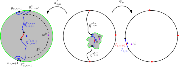
Figure 8.1: An illustration of the proof of Lemma 8.1. The arc $I_{z,n}$ and its images under various conformal maps is shown in blue. The regularity conditions in our events imply that the harmonic measure from $w$ in the middle picture of each of the black curves is uniformly positive. This is the key step in the proof of our regularity conditions for the arc $I_{z,n}$. Also shown (in red) is the arc $I_{z,n+1}$ appearing in assertion 2 and its images under the various maps.

Fix $n$, $k$, and $z$ as in the statement of the lemma. Throughout the proof we assume $E_{k}(z)$ occurs and require all constants (either referred to as such or implicit in $\asymp$, etc.) to be deterministic and independent of $n,k$, and $z\in B_{d}(0)$. See Figure 8.1 for an illustration of the argument.

The map $\pi^{\operatorname{f}}_{z,n}:D^{\operatorname{f}}_{z,n}\rightarrow\mathbf{D}$ defined in Section 7.3.2 takes $z$ to $0$ and $\eta\cap D^{\operatorname{f}}_{z,n}$ to the curve $\eta_{z,n+1}$, whose endpoints are $x_{z,n+1}$ and $y_{z,n+1}$. Note that condition 3 in the definition of $\widetilde{E}_{z,n}$ together with condition 3 in the definition of $F_{z,n}$ implies a lower bound on $|x_{z,n+1}-y_{z,n+1}|$, depending only on the parameter $a$.

Recall that $[x_{z,n+1}^{*},y_{z,n+1}^{*}]_{\partial\mathbf{D}}$ is the largest arc of $\partial\mathbf{D}$ to the right $\eta_{z,n+1}$ which does not contain a point of $\eta_{z,n+1}$ in its interior. By conditions 1 and 3 in the definition of $L_{z,n+1}$ and condition 4 in the definition of $\widetilde{E}_{z,n+1}$, there is a unique arc $A^{0}$ of $\partial\mathcal{B}_{\widetilde{\Delta}/2}$ which lies to the right of $\eta_{z,n+1}$ and which disconnects $\eta_{z,n+1}\cap\mathcal{\mathcal{missing}}B_{\widetilde{\Delta}}$ from $[x_{z,n+1}^{*},y_{z,n+1}^{*}]_{\partial\mathbf{D}}$ in $\mathbf{D}\setminus\eta_{z,n+1}$ (c.f. Remark 7.5). Let $w^{0}$ be the point of $A^{0}$ closest to the midpoint of $[x_{z,n+1}^{*},y_{z,n+1}^{*}]_{\partial\mathbf{D}}$ and let $D^{0}$ be the connected component of $\mathbf{D}\setminus\eta_{z,n+1}$ containing $[x_{z,n+1}^{*},y_{z,n+1}^{*}]_{\partial\mathbf{D}}$ on its boundary.

From the definitions of $L_{z,n+1}$ and $\widetilde{E}_{z,n+1}$, we find that the harmonic measure from $w^{0}$ in $D^{0}$ of any sub-arc of $[x_{z,n+1}^{*},y_{z,n+1}^{*}]_{\partial\mathbf{D}}$ lying at distance at least $e^{-2\Delta}$ from the endpoints is proportional to the length of that sub-arc. Furthermore, $\operatorname{hm}^{w^{0}}(\eta_{z,n+1};D^{0})\asymp 1$. Define $\psi_{z,n}:\mathbf{D}\setminus(\eta^{\tau_{z,n}}\cup\overline{\eta}^{\overline{\tau}_{z,n}})\rightarrow\mathbf{D}$ as in condition 2 in the definition of $F_{z,n}$. By condition 3 in the definition of $\widetilde{E}_{z,n}$, the arc of $\partial\mathbf{D}$ which is the image of the right side of $\eta_{z,n}^{\tau_{z,n}}$ (resp. the left side of $\overline{\eta}_{z,n}^{\overline{\tau}_{z,n}}$) under $\psi_{z,n}$ has length $\asymp 1$. By the conformal invariance of Brownian motion and condition 3 in the definition of $F_{z,n}$, the harmonic measure from $(\psi_{z,n}\circ\pi_{z,n}^{-1})(w^{0})$ in the right connected component of $\mathbf{D}\setminus\psi_{z,n}(\eta_{z,n}\setminus(\eta_{z,n}^{\tau_{z,n}}\cup\overline{\eta}_{z,n}^{\overline{\tau}_{z,n}})$ of each of these two sub-arcs is $\asymp 1$.

Let $w=(\pi_{z,n}^{\operatorname{f}})^{-1}(w^{0})$. It follows from the above considerations and conformal invariance of Brownian motion that (notation as in Section 2.1)

$$\operatorname{hm}^{w}(\eta^{\tau_{z,n}^{{\operatorname{f}},*}};D_{\eta})\asymp\operatorname{hm}^{w}(\overline{\eta}^{\overline{\tau}_{z,n}^{{\operatorname{f}},*}};D_{\eta})\asymp\operatorname{hm}^{w}(\eta\cap D_{z,n}^{\operatorname{f}};D_{\eta})\asymp 1.$$ (8.1)

By Lemma B.3 and condition 1 in the definition of $L_{z,n}$, we thus have

$$|\Psi_{\eta}^{\prime}(w)|\asymp|(\Phi^{\operatorname{f}}_{z,n})^{\prime}(w)|,\quad\operatorname{and}\quad\operatorname{dist}(w,\eta)\asymp\operatorname{dist}\left(w,\eta^{\tau_{z,n}^{{\operatorname{f}},*}}\cup\overline{\eta}^{\overline{\tau}_{z,n}^{{\operatorname{f}},*}}\right)$$ (8.2)

with $\Phi^{\operatorname{f}}_{z,n}$ the map from Lemma 7.13.

By the Koebe growth theorem applied to $(\pi_{z,n}^{\operatorname{f}})^{-1}$, we have $|w-z|\leq\frac{1}{100}\operatorname{dist}(z,\eta^{\tau_{z,n}^{{\operatorname{f}},*}}\cup\overline{\eta}^{\overline{\tau}_{z,n}^{{\operatorname{f}},*}})$ provided $\beta_{n}$ is chosen sufficiently large. By the Koebe distortion theorem, $|(\Phi^{\operatorname{f}}_{z,n})^{\prime}(w)|\asymp|(\Phi^{\operatorname{f}}_{z,n})^{\prime}(z)|$, so by (8.2) and assertion 1 of Lemma 7.13,

$$e^{-\overline{\beta}_{n}q-2\overline{u}_{n}}\preceq|(\Phi^{\operatorname{f}}_{z,n})^{\prime}(w)|\preceq e^{-\overline{\beta}_{n}q+2\overline{u}_{n}}.$$ (8.3)

Moreover, by assertion 2 of Lemma 7.13 and assertion 4 of Lemma 7.10, $\operatorname{dist}(z,\eta^{\tau_{z,n}^{{\operatorname{f}},*}}\cup\overline{\eta}^{\overline{\tau}_{z,n}^{{\operatorname{f}},*}})$ is bounded between constants times $e^{-\overline{\beta}_{n}-\overline{u}_{n}}$ and $e^{-\overline{\beta}_{n}+\overline{u}_{n}}$, so by (8.2) also

$$e^{-\overline{\beta}_{n}-\overline{u}_{n}}\preceq\operatorname{dist}(w,\eta)\preceq e^{-\overline{\beta}_{n}+\overline{u}_{n}}.$$ (8.4)

Let $\widetilde{w}=\Psi_{\eta}(w)$. By (8.3), (8.4), and the Koebe quarter theorem, $e^{-\overline{\beta}_{n}(q+1)-3\overline{u}_{n}}\preceq 1-|\widetilde{w}|\preceq e^{-\overline{\beta}_{n}(q+1)+3\overline{u}_{n}}$. By (8.1) and conformal invariance of harmonic measure,

$$\operatorname{dist}(\widetilde{w},I_{z,n})\asymp\operatorname{length}(I_{z,n})\asymp 1-|\widetilde{w}|.$$ (8.5)

This proves assertion 1.

To prove assertion 2, we observe that the harmonic measure from $w^{0}$, as defined above, of each of $\eta_{z,n+1}^{\sigma_{z,n+1}}$ and $\overline{\eta}_{z,n+1}^{\overline{\sigma}_{z,n+1}}$ is $\asymp 1$, where here $\sigma_{z,n+1}$ and $\overline{\sigma}_{z,n+1}$ are the times in the definition of $L_{z,n}$. It therefore follows from conformal invariance of harmonic measure that the distance from the endpoints of $I_{z,n}$ to the endpoints of $I_{z,n+1}$ is $\succeq 1-|\widetilde{w}|$. We conclude by means of (8.5).

To complete the proof of assertion 3, suppose given $x\in I_{z,n}$. By (8.5) the angle between the tangent line to $\partial\mathbf{D}$ at $x$ and the segment $[x,\widetilde{w}]$ is bounded away from 0 and $\pi$. Hence we can find $\delta_{n}\asymp 1-|\widetilde{w}|=e^{-\overline{\beta}_{n}(q+1+o_{n}(1))}$ and $\rho\in(0,1)$, bounded away from 0 and 1, such that $\widetilde{w}\in B_{\rho\delta_{n}}((1-\delta_{n})x)$. By the Koebe distortion theorem we have $|(\Psi_{\eta}^{-1})^{\prime}((1-\delta_{n})x)|\asymp|(\Psi_{\eta}^{-1})^{\prime}(\widetilde{w})|$. By combining this with (8.3) we conclude that assertion 3 holds. ∎

8.2 Lower bound for the Hausdorff dimension of the subset of the curve

In this subsection we will prove a lower bound on the Hausdorff dimension of the multifractal spectrum sets $\Theta^{s}(D_{\eta})\subset\eta$.

Proposition 8.2.

Let $s_{-},s_{+}$ be as in Theorem 1.1. For each $s\in(s_{-},s_{+})$, a.s.

$$\dim_{\mathcal{H}}\Theta^{s}(D_{\eta})\geq\xi(s),$$

where $\xi(s)$ is as in (1.4).

For the proof, we assume we are in the setting of Section 8.1. We first define a closed subset $\mathcal{P}$ of $\Theta^{s}(D_{\eta})$, the so-called perfect points, whose Hausdorff dimension can be bounded below using the estimates of Section 7. Let $\lambda_{*}$ be the constant from Lemma 7.13. For $n\in\mathbf{N}$, let $n^{\prime}$ be the greatest integer such that $\overline{\beta}_{n}-\lambda_{*}n\geq\overline{\beta}_{n^{\prime}+1}+\lambda_{*}(n^{\prime}+2)$. Let

$$\epsilon_{n}:=e^{-\overline{\beta}_{n^{\prime}+1}-\lambda_{*}(n^{\prime}+2)}.$$ (8.6)

Note that Lemma 7.10 implies $e^{-\overline{\beta}_{n}}=\epsilon_{n}^{1+o_{n}(1)}$. Our reason for choosing this value of $\epsilon_{n}$ is that the pockets $D_{z,n}^{\operatorname{f}}$ and $D^{\operatorname{f}}_{w,n}$ are disjoint on $E_{n}(z)\cap E_{n}(w)$ provided $|z-w|\geq\epsilon_{n}$ (see Lemma 7.13).

Choose a collection $\mathcal{C}_{n}$ of $\asymp\epsilon_{n}^{-2}$ points in $B_{d}(0)$, no two of which lie within distance $\epsilon_{n}$ of each other. Let $\mathcal{C}_{n}^{\prime}$ be the set of $z\in\mathcal{C}_{n}$ for which $E_{n}(z)$ occurs and define the perfect points by

$$\mathcal{P}:=\bigcap_{n\geq 1}\overline{\bigcup_{k\geq n}\bigcup_{z\in\mathcal{C}_{k}^{\prime}}B_{\epsilon_{k}}(z)}.$$ (8.7)

Lemma 8.3.

With $\mathcal{P}$ as in (8.7), we have $\mathcal{P}\subset\Theta^{s}(D_{\eta})$ for $s=q/(q+1)$. In fact, if $w\in\mathcal{P}$ then for $\epsilon>0$,

$$|(\Psi_{\eta}^{-1})^{\prime}((1-\epsilon)\Psi_{\eta}(w))|=\epsilon^{-s+o_{\epsilon}(1)},$$ (8.8)

with the rate of the $o_{\epsilon}(1)$ deterministic and uniform for $w\in\mathcal{P}$.

Proof.

Fix $w\in\mathcal{P}$. Since $\eta$ is closed, it is clear that $w\in\eta$. It remains to prove (8.8). By definition of $\mathcal{P}$, if we are given $n\in\mathbf{N}$, then we can find $k\geq n+1$ and $z\in\mathcal{C}_{k}^{\prime}$ such that $|z-w|\leq e^{-2\overline{\beta}_{n+1}}$. By Lemma 7.13, $w\in D^{\operatorname{f}}_{z,n}$ so $\Psi_{\eta}(w)\in I_{z,n}$, as defined in Lemma 8.1. Let $\delta_{n}$ be as in that lemma with $x=\Psi_{\eta}(w)$.

By the Koebe distortion theorem, for $\epsilon\in[\delta_{n+1},\delta_{n}]$,

$$\frac{1-(\delta_{n}-\delta_{n+1})/\delta_{n}}{(1+(\delta_{n}-\delta_{n+1})/\delta_{n})^{3}}\leq\frac{|(\Psi_{\eta}^{-1})^{\prime}((1-\epsilon)\Psi_{\eta}(w))|}{|(\Psi_{\eta}^{-1})^{\prime}((1-\delta_{n})\Psi_{\eta}(w))|}\leq\frac{1+(\delta_{n}-\delta_{n+1})/\delta_{n}}{(1-(\delta_{n}-\delta_{n+1})/\delta_{n})^{3}}.$$ (8.9)

Since $\delta_{n}=e^{-\overline{\beta}_{n}(q+1+o_{n}(1))}$ (condition 3 of Lemma 8.1),

$$1-(\delta_{n}-\delta_{n+1})/\delta_{n}=e^{-\beta_{n+1}(q+1+o_{n}(1))}=e^{\overline{\beta}_{n}o_{n}(1)},$$

which is proportional to $\epsilon^{o_{\epsilon}(1)}$ by Lemma 7.10. We furthermore have $\delta_{n}=\epsilon^{1+o_{\epsilon}(1)}$. Hence (8.9) and condition 3 of Lemma 8.1 imply $|(\Psi_{\eta}^{-1})^{\prime}((1-\epsilon)\Psi_{\eta}(w))|=\epsilon^{-s+o_{\epsilon}(1)}$, as required. ∎

Proof of Proposition 8.2.

For a Borel measure $\nu$ on a metric space $X$ and $\alpha>0$, write

$$I_{\alpha}(\nu)=\int_{X}\int_{X}\frac{d\nu(z)\,d\nu(w)}{|z-w|^{\alpha}}$$ (8.10)

for the $\alpha$-energy of $\nu$. By standard results for Hausdorff dimension (see [MP10, Theorem 4.27]) a metric space which admits a positive finite measure with finite $\alpha$-energy has Hausdorff dimension at least $\alpha$. In view of Lemma 8.3, we are led to construct such a measure $\nu$ on $\mathcal{P}$ for each $\alpha<\xi(s)$. We do this using the usual argument (see, e.g. [MW17, HMP10, Bef08]) and the estimates of Section 7.5

Define the events $E_{n}(z)$ as in Section 7.3 and the sets of points $\mathcal{C}_{n}$ and $\mathcal{C}_{n}^{\prime}$ as in the definition of $\mathcal{P}$ (right above (8.7)). Let $\epsilon_{n}$ be as in (8.6).

For each $n\in\mathbf{N}$, define a measure $\nu_{n}$ on $\mathbf{D}$ by

$$d\nu_{n}(x)=\sum_{z\in\mathcal{C}_{n}}\frac{\mathbf{1}_{E_{n}(z)}}{\mathbf{P}(E_{n}(z))}\mathbf{1}_{(x\in B_{\epsilon_{n}}(z))}\,dx.$$

Then $\mathbf{E}(\nu_{n}(\mathbf{D}))\asymp 1$. Moreover,

$$\mathbf{E}(\nu_{n}(\mathbf{D})^{2}) \preceq\epsilon_{n}^{4}\sum_{\begin{subarray}{c}z,w\in\mathcal{C}_{n},\\ z\not=w\end{subarray}}\frac{\mathbf{P}(E_{n}(z)\cap E_{n}(w))}{\mathbf{P}(E_{n}(z))\mathbf{P}(E_{n}(w))}+\epsilon_{n}^{4}\sum_{z\in\mathcal{C}_{n}}\frac{1}{\mathbf{P}(E_{n}(z))}.$$

By Lemma 7.12 and Proposition 7.17 (c.f. Remark 7.18), this is bounded by an $n$-independent constant times

$$\epsilon_{n}^{4}\sum_{\begin{subarray}{c}z,w\in\mathcal{C}_{n},\\ z\not=w\end{subarray}}|z-w|^{-\gamma^{*}(q)+o_{|z-w|}(1)}+\epsilon_{n}^{4}\sum_{z\in\mathcal{C}_{n}}\epsilon_{n}^{-\gamma^{*}(q)+o_{n}(1)},$$

with the $o_{|z-w|}(1)$ tending to $0$ as $|z-w|\rightarrow 0$, at a rate which is independent of the particular locations of $z$ and $w$ and of $n$. For $s\in(s_{-},s_{+})$ we have $\gamma^{*}(q)=\gamma(s)/(1-s)<2$. Therefore, for sufficiently large $n$, $\mathbf{E}(\nu_{n}(\mathbf{D})^{2})$ is bounded above by a finite, $n$-independent constant. By the Vitalli convergence theorem, we can a.s. find a subsequence of the measures $\nu_{n}$ which converges weakly to a measure $\nu$ whose total mass is bounded above by some deterministic constant, and whose expected mass is positive.

On the other hand, we have

$$\mathbf{E}(I_{\alpha}(\nu_{n})) =\sum_{z,w\in\mathcal{C}_{n}}\frac{\mathbf{P}(E_{n}(z)\cap E_{n}(w))}{\mathbf{P}(E_{n}(z))\mathbf{P}(E_{n}(w))}\iint_{B_{\epsilon_{n}}(z)\times B_{\epsilon_{n}}(w)}\frac{1}{|x-y|^{\alpha}}\,dx\,dy$$

$$=\sum_{\begin{subarray}{c}z,w\in\mathcal{C}_{n},\\ z\not=w\end{subarray}}\frac{\mathbf{P}(E_{n}(z)\cap E_{n}(w))}{\mathbf{P}(E_{n}(z)E_{n}(z))\mathbf{P}(E_{n}(z))}\iint_{B_{\epsilon_{n}}(z)\times B_{\epsilon_{n}}(w)}\frac{1}{|x-y|^{\alpha}}\,dx\,dy$$

$$+\sum_{z\in\mathcal{C}_{n}}\frac{1}{\mathbf{P}(E_{n}(z))}\iint_{B_{\epsilon_{n}}(z)\times B_{\epsilon_{n}}(z)}\frac{1}{|x-y|^{\alpha}}\,dx\,dy$$

$$\preceq\sum_{\begin{subarray}{c}z,w\in\mathcal{C}_{n},\\ z\not=w\end{subarray}}\frac{\mathbf{P}(E_{n}(z)\cap E_{n}(w))}{\mathbf{P}(E_{n}(z))\mathbf{P}(E_{n}(z))}\frac{\epsilon_{n}^{4}}{|z-w|^{\alpha}}+\sum_{z\in\mathcal{C}_{n}}\frac{\epsilon_{n}^{4-\alpha}}{\mathbf{P}(E_{n}(z))}$$

$$\preceq\sum_{\begin{subarray}{c}z,w\in\mathcal{C}_{n},\\ z\not=w\end{subarray}}|z-w|^{-\gamma^{*}(q)-\alpha+o_{|z-w|}(1)}\epsilon_{n}^{4}+\epsilon_{n}^{2-\alpha-\gamma^{*}(q)+o_{n}(1)}.$$

We have $\gamma^{*}(q)+\alpha<2$ for $s\in(s_{-},s_{+})$ and $\alpha<\xi(s)$, so the above expression is $\preceq 1$. We conclude that with positive probability, there exists a weak subsequential limit $\nu$ of the measures $(\nu_{n})$ supported on $\mathcal{P}$ and satisfying $\nu(\mathcal{P})>0$ and $I_{\alpha}(\nu)<\infty$. Hence [MP10, Theorem 4.27] and Lemma 8.3 imply that with positive probability, we have $\dim_{\mathcal{H}}\Theta^{s}(D_{\eta})\geq\xi(s)$. Proposition 2.15 implies that this in fact a.s. holds. ∎

8.3 Lower bound for the Hausdorff dimension of the subset of the circle

In this subsection we prove the following lower bound for the set Hausdorff dimension of the set $\widetilde{\Theta}^{s}(D_{\eta})=\Psi_{\eta}^{-1}(\Theta^{s}(D_{\eta}))\subset\partial\mathbf{D}$.

Proposition 8.4.

Let $s_{-},s_{+}$ be as in Theorem 1.1. For each $s\in(s_{-},s_{+})$, a.s.

$$\dim_{\mathcal{H}}\widetilde{\Theta}^{s}(D_{\eta})\geq\widetilde{\xi}(s),$$

where $\widetilde{\xi}(s)$ is as in (1.3).

For the proof of Proposition 8.4, we will need a different set of perfect points. Define $\epsilon_{n}$, the sets $\mathcal{C}_{n}$, $\mathcal{C}_{n}^{\prime}$ as in the definition (8.7) of $\mathcal{P}$. For $z\in\mathcal{C}_{n}^{\prime}$, let $I_{z,n-1}$ be as in the statement of Lemma 8.1. Let $v_{z,n}$ be the midpoint of $I_{z,n-1}$ and let $I_{z,n}^{\prime}$ be the arc of length $\epsilon_{n}^{q+1}$ centered at $v_{z,n}$. By Lemma 8.1, $\operatorname{length}(I_{z,n}^{\prime})=\operatorname{length}(I_{z,n-1})^{1+o_{n}(1)}$. Our perfect points in this case are defined by

$$\widetilde{\mathcal{P}}:=\bigcap_{n\geq 1}\overline{\bigcup_{k\geq n}\bigcup_{z\in\mathcal{C}_{k}^{\prime}}I_{z,k-1}^{\prime}}.$$ (8.11)

Our first task is to check that $\widetilde{\mathcal{P}}\subset\widetilde{\Theta}^{s}(D_{\eta})$.

Lemma 8.5.

Define $\widetilde{\mathcal{P}}$ as in (8.11). If the auxiliary parameter $\widetilde{\Delta}$ (Definition 7.1) and the value $\beta_{0}$ are chosen sufficiently large then $\widetilde{\mathcal{P}}\subset\widetilde{\Theta}^{s}(D_{\eta})$ for $s=q/(q+1)$. In fact, if $x\in\widetilde{\mathcal{P}}$, then for $\epsilon>0$,

$$|(\Psi_{\eta}^{-1})^{\prime}((1-\epsilon)x)|=\epsilon^{-s+o_{\epsilon}(1)},$$

with the implicit constants and the $o_{\epsilon}(1)$ deterministic and uniform in $x$.

Proof.

If $x\in\widetilde{\mathcal{P}}$ then for any $n\in\mathbf{N}$ we can find $k\geq n$ and $z\in\mathcal{C}_{k}^{\prime}$ such that $x$ lies within distance $\operatorname{length}(I_{z,n}^{\prime})^{2}$ of $I_{z,k}^{\prime}$. If $k$ is chosen sufficiently large, depending on $n$, then by assertions 1 and 2 of Lemma 8.1 we have $x\in I_{z,n}$. We then conclude as in the proof of Lemma 8.3. ∎

In the proof of Proposition 8.4, we will break up the sum which gives the second moment of our measures into three terms, depending on the distance between the points under consideration. The following lemma is needed to bound the number of pairs of points at mesoscopic distance.

Lemma 8.6.

For each $n\in\mathbf{N}$ there is an integer $m_{n}\leq n$ such that the following is true. We have $\overline{\beta}_{n}-\overline{\beta}_{m_{n}}=\overline{\beta}_{n}o_{n}(1)$ and if $z,w\in\mathcal{C}_{n}^{\prime}$ with $|z-w|\geq e^{-\overline{\beta}_{m_{n}+1}}$ then $\operatorname{dist}(I_{z,n}^{\prime},I_{w,n}^{\prime})\succeq|z-w|^{q+1+o_{|z-w|}(1)}$, with the $o_{|z-w|}(1)$ and implicit constants deterministic, independent of $n$, and independent of the particular choices of $z$ and $w$ in $\mathcal{C}_{n}^{\prime}$.

Proof.

We argue as in the proof of Lemma 7.21. Choose $k\in\mathbf{N}$ such that $e^{-\beta_{k+1}-\lambda_{*}(k+1)}\leq|z-w|\leq e^{-\beta_{k}-\lambda_{*}k}$. Let $k^{\prime}$ be the least integer such that $\overline{\beta}_{k^{\prime}}-\lambda_{*}k^{\prime}\geq\overline{\beta}_{k+1}+\lambda_{*}(k+1)$. By our choice (8.6) of $\epsilon_{n}$ we have $k^{\prime}\leq n-1$. By Lemma 7.13, $D^{\operatorname{f}}_{z,k^{\prime}}\cap D^{\operatorname{f}}_{w,k^{\prime}}=\emptyset$ and hence $I_{z,k^{\prime}}\cap I_{w,k^{\prime}}=\emptyset$. If $\operatorname{length}(I_{z,n}^{\prime})\leq\operatorname{length}(I_{z,k^{\prime}+1})$ then by assertions 1 and 2 of Lemma 8.1, the midpoints of $I_{z,n^{\prime}}$ and $I_{w,n}^{\prime}$ satisfy

$$\operatorname{dist}(v_{z,n},v_{w,n})\succeq e^{-\overline{\beta}_{k^{\prime}+1}(q+1)-3\overline{u}_{k^{\prime}+1}}\succeq|z-w|^{q+1+o_{|z-w|}(1)}.$$

On the other hand, by assertion 1 of Lemma 8.1 we have $\operatorname{length}(I_{z,n}^{\prime})\leq\operatorname{length}(I_{z,k^{\prime}+1})$ provided $\overline{\beta}_{k^{\prime}+1}(q+1)+3\overline{u}_{k^{\prime}+1}\leq(\overline{\beta}_{n}-\lambda_{*}n+\overline{\beta}_{n}o_{n}(1))(q+1)$, or equivalently provided

$$\overline{\beta}_{n}-\overline{\beta}_{k^{\prime}+1}\geq\frac{3\overline{u}_{k^{\prime}+1}+\lambda_{*}n+\overline{\beta}_{n}o_{n}(1)}{q+1}.$$

It follows from Lemma 7.10 that we can choose $m_{n}\leq n$ such that $\overline{\beta}_{n}-\overline{\beta}_{m_{n}}=\overline{\beta}_{n}o_{n}(1)$ and $\operatorname{length}(I_{z,n}^{\prime})\leq\operatorname{length}(I_{z,k^{\prime}+1})$ whenever $k^{\prime}\leq m_{n}$. ∎

Proof of Proposition 8.4.

We argue as in the proof of Proposition 8.2. In particular, for any given $\alpha<\widetilde{\xi}(s)$, we will construct a positive finite measure $\widetilde{\nu}$ on $\widetilde{\mathcal{P}}$ (as defined in (8.11)) with finite $\alpha$-energy (as defined in (8.10)).

Define $\epsilon_{n}$ as in (8.6). We require all implicit constants and $o_{|z-w|}(1)$ terms to be independent of $n$ and uniform for $z,w\in\mathcal{C}_{n}$. For $n\in\mathbf{N}$, define a measure $\widetilde{\nu}_{n}$ on $\partial\mathbf{D}$ by

$$d\widetilde{\nu}_{n}(x)=\epsilon_{n}^{1-q}\sum_{z\in\mathcal{C}_{n}^{\prime}}\frac{\mathbf{1}_{E_{n}(z)}}{\mathbf{P}(E_{n}(z))}\mathbf{1}_{(x\in I_{z,k}^{\prime})}\,dx.$$

Then we have $\mathbf{E}(\widetilde{\nu}_{n}(\partial\mathbf{D}))\asymp 1$.

As in the proof of Proposition 8.2,

$$\mathbf{E}(\widetilde{\nu}_{n}(\partial\mathbf{D})^{2}) \preceq\epsilon_{n}^{4}\sum_{\begin{subarray}{c}z,w\in\mathcal{C}_{n},\\ z\not=w\end{subarray}}\frac{\mathbf{P}(E_{n}(z)\cap E_{n}(w))}{\mathbf{P}(E_{n}(z))\mathbf{P}(E_{n}(w))}+\epsilon_{n}^{4}\sum_{z\in\mathcal{C}_{n}}\epsilon_{n}^{-\gamma^{*}(q)+o_{n}(1)}\preceq 1.$$

Let $m_{n}$ be as in Lemma 8.6 and let $\mathcal{K}_{n}$ be the set of pairs $(z,w)\in\mathcal{C}_{n}\times\mathcal{C}_{n}$ with $|z-w|\leq e^{-\overline{\beta}_{m_{n}}}$ and $z\not=w$. By Lemma 8.6 we have $\#\mathcal{K}_{n}\leq\epsilon_{n}^{-2-o_{n}(1)}$.

By Lemma 7.12, Proposition 7.17, and Lemma 8.6,

$$\mathbf{E}(I_{\alpha}(\widetilde{\nu}_{n})) =\epsilon_{n}^{2-2q}\sum_{(z,w)\in\mathcal{C}_{n}\times\mathcal{C}_{n}}\frac{\mathbf{P}(E_{n}(z)\cap E_{n}(w))}{\mathbf{P}(E_{n}(z))\mathbf{P}(E_{n}(w))}\iint_{I_{z,k}^{\prime}\times I_{w,k}^{\prime}}\frac{1}{|x-y|^{\alpha}}\,dx\,dy$$

$$\preceq\sum_{(z,w)\notin\mathcal{K}_{n},\>z\not=w}|z-w|^{-\gamma^{*}(q)+o_{|z-w|}(1)}|v_{z,n}-v_{w,n}|^{-\alpha}\epsilon_{n}^{2(q+1)+2-2q}$$

$$+\sum_{(z,w)\in\mathcal{K}_{n}}|z-w|^{-\gamma^{*}(q)+o_{|z-w|}(1)}\epsilon_{n}^{(2-\alpha)(q+1)+2-2q+o_{n}(1)}$$

$$+\sum_{z\in\mathcal{C}_{n}}\epsilon_{n}^{(2-\alpha)(q+1)+2-2q-\gamma^{*}(q)+o_{n}(1)}$$

$$\preceq\epsilon_{n}^{4}\sum_{\begin{subarray}{c}z,w\in\mathcal{C}_{n},\\ z\not=w\end{subarray}}|z-w|^{-\gamma^{*}(q)-\alpha(q+1)+o_{|z-w|}(1)}+\epsilon_{n}^{(2-\alpha)(q+1)-2q-\gamma^{*}(q)+o_{n}(1)}+\epsilon_{n}^{(2-\alpha)(q+1)-2q-\gamma^{*}(q)+o_{n}(1)}.$$

Note that for the middle term we used $|z-w|\succeq\epsilon_{n}$ and $\#\mathcal{K}_{n}\leq\epsilon_{n}^{-2-o_{n}(1)}$. If $s\in(s_{-},s_{+})$ and $q=s/(1-s)$ we have $\gamma^{*}(q)+\alpha(q+1)<2$ and $(2-\alpha)(1+q)-2q-\gamma^{*}(q)>0$ for $\alpha<\widetilde{\xi}(s)$. It follows that we can a.s. find a subsequence of the measures $(\widetilde{\nu}_{n})$ which converges weakly to a finite positive limiting measure supported on $\widetilde{\mathcal{P}}$ with finite $\alpha$-energy. We then conclude using [MP10, Theorem 4.27], Lemma 8.5, and Proposition 2.15. ∎

8.4 Proof of Theorem 1.1

This follows by combining Propositions 5.1, 5.6, 8.2, and 8.4. ∎

Remark 8.7.

In the case $\kappa=4$, we have $s_{+}=1$, so the sets $\Theta^{1}(D_{\eta})$ and $\widetilde{\Theta}^{1}(D_{\eta})$ for $\kappa=4$ can be non-empty. We do not explicitly mention these sets in Theorem 1.1 because our results do not apply in full in this case. However, we do prove something about these sets. In particular, we prove in Proposition 5.1 that a.s. $\dim_{\mathcal{H}}\widetilde{\Theta}^{1}(D_{\eta})=0$. Since $\dim_{\mathcal{H}}(\eta)=3/2$ for $\kappa=4$, we get a trivial upper bound of $3/2$ for $\dim_{\mathcal{H}}\Theta^{1}(D_{\eta})$ in the case $\kappa=4$. We do not prove a lower bound for $\dim_{\mathcal{H}}\Theta^{1}(D_{\eta})$ in this paper, and we are not sure if the upper bound of $3/2$ is optimal.

8.5 Lower bound for the integral means spectrum

In this subsection we prove our lower bound for the bulk integral means spectrum of the SLE curve and thereby complete the proof of Corollary 1.9.

Proof of Corollary 1.9.

Throughout, we consider a fixed realization and allow implicit constants to be random (but independent of the parameters of interest).

Fix $s\in[s_{-},s_{+}]$ (as defined in (1.5) and (1.6)) to be chosen later, and let $\widetilde{\mathcal{P}}$ be the set of perfect points defined in (8.11). Also fix $\alpha<\widetilde{\xi}(s)$. By the proof of Proposition 8.4, the probability of the event

$$E:=\{\dim_{\mathcal{H}}\widetilde{\mathcal{P}}>\alpha\}$$

is positive. Moreover, it is clear from the definition that $\widetilde{\mathcal{P}}\subset\Psi_{\eta}^{-1}(\eta\cap B_{d}(0))$. The idea of the proof is that on $E$, we have a lower bound for the size of the set of $x\in\partial\mathbf{D}$ where $|\Psi_{\eta}^{\prime}((1-\epsilon)x)|$ grows like $\epsilon^{-s}$, which gives us a lower bound for the integral of $|\Psi_{\eta}^{\prime}|^{a}$ over $\partial B_{1-\epsilon}(0)$. We then optimize over $s$ to get a lower bound for the integral means spectrum.

For $n\in\mathbf{N}$ let $\widehat{\epsilon}_{n}:=2^{-n}$. Let $\mathcal{I}_{n}$ be the collection of arcs $[e^{2\pi i(k-1)\widehat{\epsilon}_{n}},e^{2\pi ik\widehat{\epsilon}_{n}}]_{\partial\mathbf{D}}$ for $k\in\{1,\dots,2^{n}\}$ and let $\mathcal{I}_{n}^{\prime}$ be the set of those arcs $I\in\mathcal{I}_{n}$ which intersect $\widetilde{\mathcal{P}}$. Then $\mathcal{I}_{n}^{\prime}$ is a cover of $\widetilde{\mathcal{P}}$ consisting of sets of diameter at most $O_{n}(\widehat{\epsilon}_{n})$. Hence on $E$ we have $(\#\mathcal{I}_{n}^{\prime})\widehat{\epsilon}_{n}^{\alpha}\succeq 1$ (with possibly random, but $n$-independent implicit constant) so $\#\mathcal{I}_{n}^{\prime}\succeq\widehat{\epsilon}_{n}^{-\alpha}$.

For $I\in\mathcal{I}_{n}^{\prime}$ choose $x_{I}\in I\cap\widetilde{\mathcal{P}}$ and let $z_{I}=(1-\widehat{\epsilon}_{n})x_{I}$. By Lemma 8.5, $|(\Psi_{\eta}^{-1})^{\prime}(z_{I})|\succeq\widehat{\epsilon}_{n}^{-s+o_{n}(1)}$, with the $o_{n}(1)$ and the implicit constant independent of the choice of $I$ and $x_{I}$.

Let $J_{I}$ be the intersection of $(1-\widehat{\epsilon}_{n})I$ with the arc of $\partial B_{1-\widehat{\epsilon}_{n}}(0)$ centered at $z_{I}$ of length $\widehat{\epsilon}_{n}^{1+r_{n}}$, where $(r_{n})$ is a sequence of positive numbers with $r_{n}\rightarrow 0$ slower than the $o_{n}(1)$ above. Then the arcs $J_{I}$ are disjoint for sufficiently large $n$ and by the Koebe distortion theorem we have $|(\Psi_{\eta}^{-1})^{\prime}(w)|\succeq\widehat{\epsilon}_{n}^{s+o_{n}(1)}$ for each $w\in J_{I}$. Each point of $\widetilde{\mathcal{P}}$ is mapped into $B_{1-d/2}(0)$ by $\Psi_{\eta}^{-1}$. Hence for sufficiently large $n$ and sufficiently small $\zeta$ (random), we have $J_{I}\subset A_{\widehat{\epsilon}_{n}}^{\zeta}(\Psi_{\eta}^{-1})$ for each $I\in\mathcal{I}_{n}^{\prime}$, with $A_{\widehat{\epsilon}_{n}}^{\zeta}(\Psi_{\eta}^{-1})$ defined just below (1.10) with $\phi=\Psi_{\eta}^{-1}$. Hence on $E$, it holds for $a\in\mathbf{R}$ that

$$\int_{A_{\widehat{\epsilon}_{n}}^{\zeta}(\Psi_{\eta}^{-1})}|(\Psi_{\eta}^{-1})^{\prime}(w)|^{a}\,dw\succeq\sum_{I\in\mathcal{I}_{n}^{\prime}}\int_{J_{I}}|(\Psi_{\eta}^{-1})^{\prime}(w)|^{a}\,dw\succeq\widehat{\epsilon}_{n}^{-\alpha-as+1+o_{n}(1)}.$$

Therefore, for any $a\in\mathbf{R}$, on $E$ it holds that

$$\limsup_{n\rightarrow\infty}\frac{\log\int_{A_{\widehat{\epsilon}_{n}}^{\zeta}(\Psi_{\eta}^{-1})}|(\Psi_{\eta}^{-1})^{\prime}(w)|^{a}\,dw}{\log\widehat{\epsilon}_{n}^{-1}}\geq\alpha+as-1.$$

Thus $\operatorname{IMS}_{D_{\eta}}^{\operatorname{bulk}}(a)\geq\alpha+as-1$ with positive probability.

By Proposition 2.16, this lower bound in fact holds a.s. Since $\alpha<\widetilde{\xi}(s)$ is arbitrary, it follows that a.s.

$$\operatorname{IMS}_{D_{\eta}}^{\operatorname{bulk}}(a)\geq\widetilde{\xi}(s)+as-1$$ (8.12)

In the notation of Corollary 1.9, this quantity is maximized over all $s\in[s_{-},s_{+}]$ by taking $s=s_{*}(a)$ if $a\in[a_{-},a_{+}]$; $s=s_{-}$ if $a<a_{-}$; and $s=s_{+}$ if $a>a_{+}$. Choosing this value of $s$ in (8.12) gives us that the lower bound in (1.14) holds a.s. for each fixed $a\in\mathbf{R}$ in the case $\kappa\leq 4$, $\underline{\rho}=0$, and $V=D_{\eta}$.

By Proposition 2.16, this lower bound in fact holds a.s. for each choice of $\kappa>0$, vector of weights $\underline{\rho}$, $t>0$, and complementary connected component $V$ of $\eta([0,t])$. By combining this with Proposition 5.7, we get that (1.14) holds a.s. for each fixed $a\in\mathbf{R}$ for each choice of $\kappa>0$, vector of weights $\underline{\rho}$, $t>0$, and complementary connected component $V$ of $\eta([0,t])$. By Hölder’s inequality, it follows that the bulk integral means spectrum is a convex, hence continuous, function of $a$ (c.f. [Mak98, Theorem 5.2] for a related, but much stronger, statement for the ordinary integral means spectrum). It follows that in fact 1.14 holds a.s. for all $a\in\mathbf{R}$ simultaneously. ∎

Appendix A Proof of Proposition 3.10

In this appendix we will prove Proposition 3.10, which is one of the ingredients in the proof of Theorem 3.1. The proof will be completed in two stages. First, we will show that we can move the force point to the imaginary axis without any pathological behavior (Lemma A.1). Then, we will use a forward/reverse SLE symmetry argument to rule out pathological behavior after the force point has reached the imaginary axis. See Figure A.1 for an illustration.

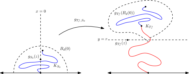
Figure A.1: An illustration of the proof of Proposition 3.10. First, we run the reverse Loewner flow with a force point at $z$ until the first time $S_{0}$ that $z$ is mapped to a point on the imaginary axis. We show in Section A.1 that for each $\zeta>0$, it holds with uniformly positive probability (independent of the particular choice of $z$) that $S_{0}\leq\zeta$, $Y_{S_{0}}=\operatorname{Im}g_{S_{0}}(z)\leq 5\zeta^{1/2}$, and $K_{S_{0}}\subset B_{d}(0)$ for some $d>0$ independent of the particular choice of $z$. Once we condition on the reverse Loewner flow up until time $S_{0}$, the law of the maps $g_{S_{0},v+S_{0}}$ which satisfy $g_{S_{0},v+S_{0}}\circ g_{S_{0}}=g_{v+S_{0}}$ for $v\geq 0$ is that of a reverse $\operatorname{SLE}_{\kappa}(\rho)$ Loewner flow with force point at $Z_{S_{0}}=g_{S_{0}}(z)$. In Section A.2, we show that the first time that the force point for such a Loewner flow reaches the line $\{\operatorname{Im}w=r\}$ (i.e., $T_{r}^{z}-S_{0}$) is bounded independently of $Z_{S_{0}}$ with high probability. Furthermore, the conformal map $g_{S_{0},T_{r}^{z}}$ is likely to “push” $B_{d}(0)\cap\mathbf{H}$ (and hence also $K_{S_{0}}$) away from the real axis; and the hull of this map (shown in red) is unlikely to be too large. These latter conditions together with Lemma 2.4 imply that $G(g_{T_{r}^{z}}^{-1},\mu)$ occurs with uniformly positive probability for appropriate choice of $\mu$.

We adopt the following notation. Fix $z\in\mathbf{H}$ with $|\operatorname{Re}z|\leq R$ and $\operatorname{Im}z=\epsilon$. Let

$$Z_{t}=g_{t}(z)=X_{t}+iY_{t}.$$ (A.1)

By (3.7), we have that under $\mathbf{P}_{*}^{z}$,

$$dX_{t}=(\rho-2)\frac{X_{t}}{|Z_{t}|^{2}}\,dt-\sqrt{\kappa}dB_{t}^{z},\qquad dY_{t}=\frac{2Y_{t}}{|Z_{t}|^{2}}\,dt,\qquad X_{0}=\operatorname{Re}z,\qquad Y_{0}=\epsilon$$ (A.2)

for $B_{t}^{z}$ a $\mathbf{P}_{*}^{z}$-Brownian motion. Also let

$$S_{0}:=\inf\{t\geq 0:X_{t}=0\}.$$ (A.3)

A.1 Pushing the force point to the imaginary axis

In this subsection we will prove the following lemma, which deals with the setup on the left side in Figure A.1.

Lemma A.1.

Suppose we are in the setting of Proposition 3.10. Let $Z_{t}=X_{t}+iY_{t}$ be as in (A.1) and let $S_{0}$ be as in (A.3). For each $\zeta\in(0,1)$, there exists $d>0$ and $p_{0}>0$, independent of $\epsilon$ and of $X_{0}\in[-R,R]$, such that the $\mathbf{P}_{*}^{z}$-probability of the event

$$E_{0}=E_{0}(z,d):=\left\{S_{0}\leq\zeta,\,Y_{S_{0}}\leq 5\zeta^{1/2},\,K_{S_{0}}\subset B_{d}(0)\right\}$$ (A.4)

is at least $p_{0}$.

Proof.

By symmetry we can assume without loss of generality that $\operatorname{Re}z=X_{0}>0$. We will treat the conditions in the definition of $E_{0}$ in order. Let

$$\nu>1\wedge\left(\frac{2(\rho-2)}{\kappa}+1\right)$$ (A.5)

and let $\widetilde{X}$ be $\sqrt{\kappa}$ times a Bessel process driven by $-B_{t}^{z}$, started from $X_{0}$, of dimension $\nu$. From the form of the SDE (A.2), one sees that a.s.

$$\widetilde{X}_{t}\geq X_{t},\quad\forall t\leq S_{0}.$$ (A.6)

Our choice (3.9) for $\rho$ implies that (A.5) holds for some Bessel dimension $\nu\in(0,2)$, in which case $\widetilde{X}$ hits $0$ before time $\zeta$ with uniformly positive probability [Law05, Proposition 1.21]. Hence we can find $p_{0}>0$ independent of $\epsilon$ and uniform for $X_{0}\in[-R,R]$ such that

$$\mathbf{P}_{*}^{z}\left(S_{0}\leq\zeta\right)\geq 2p_{0}.$$ (A.7)

By (A.2), $Y$ is increasing and $\partial_{t}Y_{t}^{2}\leq 4$. Hence $Y_{t}\leq 4t^{1/2}+\epsilon$, so on the event $\{S_{0}\leq\zeta\}$ we have $Y_{S_{0}}\leq 5\zeta^{1/2}$.

It remains to deal with the condition $\{K_{S_{0}}\subset B_{d}(0)\}$. Let $\widetilde{X}$ be the Bessel process of dimension $\nu$ started from $X_{0}$ driven by $-B_{t}^{z}$, as above. Since $\widetilde{X}$ and $B^{z}$ are a.s. bounded up to time $\zeta$ and their laws do not depend on $\epsilon$, it follows from (A.6) and (A.7) that we can find $C_{0}>0$, independent of $\epsilon$ and uniform for $X_{0}\in[-R,R]$ such that the probability of the event

$$E_{0}^{*}:=\left\{S_{0}\leq\zeta,\,Y_{S_{0}}\leq 5\zeta^{1/2},\,\sup_{t\leq\zeta}|\sqrt{\kappa}B_{t}^{z}|\leq C_{0},\,\sup_{t\leq\zeta}|X_{t}|\leq C_{0}\right\}$$

is at least $p_{0}$.

By (A.2), for $t\leq S_{0}$ it holds that

$$|\rho-2|\int_{0}^{t}\frac{X_{v}}{X_{v}^{2}+Y_{v}^{2}}\,dv\leq|X_{0}|+|X_{t}|+|\sqrt{\kappa}B_{t}|.$$ (A.8)

In the case $\rho\not=2$, it follows from (A.8) that on the event $E_{0}^{*}$,

$$\int_{0}^{t}\frac{X_{v}}{X_{v}^{2}+Y_{v}^{2}}\,dv\leq C_{1}:=\frac{R+2C_{0}}{|\rho-2|}.$$ (A.9)

In the case $\rho=2$, it follows from (A.2) that $X$ is a constant times a Brownian motion, so in this case we can (using (A.7)) find a possibly larger constant $C_{1}$, still independent of $\epsilon$, such that (A.9) holds with probability at least $1-p_{0}/2$. In this case we add this latter condition to the event $E_{0}^{*}$ (and replace $p_{0}$ with $p_{0}/2$).

Now consider some $b\in\mathbf{R}$ with $|b|>1$. Let $\delta>0$ and let $\tau_{b}$ be the first time $t$ that $|g_{t}(b)|\leq\delta$. By (3.7) and the reverse Loewner equation,

$$g_{t}(b)=-\int_{0}^{t}\frac{2}{g_{v}(b)}\,dv+\rho\int_{0}^{t}\frac{X_{v}}{X_{v}^{2}+Y_{v}^{2}}\,dv-\sqrt{\kappa}B_{t}^{z}+b.$$

So, it follows from (A.9) that on $E_{0}^{*}$,

$$\inf_{t\leq S_{0}\wedge\tau_{b}}|g_{t}(b)|\geq|b|-C_{2},$$

where

$$C_{2}=2\zeta\delta^{-1}+|\rho|C_{1}+C_{0}.$$

Hence if we take $|b|>2C_{2}$, then we have $\inf_{t\leq S_{0}\wedge\tau_{b}}|g_{t}(b)|\geq C_{2}$, which implies $\tau_{b}>S_{0}$ (provided we choose $\delta<C_{0}$).

In particular, if $b>1$ is chosen sufficiently large (independent of $\epsilon$ and $X_{0}\in[-R,R]$), then $g_{S_{0}}(-b)$ and $g_{S_{0}}(b)$ lie in $\mathbf{R}$. Therefore the map $g_{S_{0}}^{-1}$ takes $\partial K_{\tau}$ into $[-b,b]$. This implies that the harmonic measure from $\infty$ of $K_{\tau}$ in $\mathbf{H}\setminus K_{\tau}$ is at most $2\pi b$, so by [Law05, Equation 3.14], it follows that $\operatorname{diam}K_{S_{0}}$ is bounded by a constant independent of $\epsilon$ and $X_{0}\in[-R,R]$ on $E_{0}^{*}$. Since $\mathbf{P}_{*}^{z}(E_{0}^{*})\geq p_{0}$, the lemma follows. ∎

A.2 Pushing the force point starting from the imaginary axis

In light of the strong Markov property and Lemma A.1, we now need to consider the behavior of the process (A.2) if we start $(X_{0},Y_{0})$ from $(0,y)$ for $y\in[\epsilon,5\zeta^{1/2}]$ and $\zeta$ as in Lemma A.1. For this, we first need to review some calculations from [DMS14, Section 3]. Throughout this subsection, we assume $X_{0}=0$ and $Y_{0}=y\in[\epsilon,5\zeta^{1/2}]$. Let

$$\theta_{t}=\operatorname{arg}Z_{t}\quad\operatorname{and}\quad\mathfrak{t}_{y}=\frac{1}{2}\log y.$$ (A.10)

For $\mathfrak{t}\geq\mathfrak{t}_{y}$ define $\sigma(\mathfrak{t})$ by

$$\mathfrak{t}=\int_{0}^{\sigma(\mathfrak{t})}\frac{1}{|Z_{v}|^{2}}\,dv+\mathfrak{t}_{y},$$ (A.11)

so $d\sigma(\mathfrak{t})=|Z_{\sigma(\mathfrak{t})}|^{2}\,d\mathfrak{t}$ and $\sigma(\mathfrak{t}_{y})=0$. Denote processes under the time change $t=\sigma(\mathfrak{t})$ by a star, so $\theta_{\mathfrak{t}}^{*}=\theta_{\sigma(\mathfrak{t})}$, etc. By some elementary calculations using Itô’s formula (see the proof of [DMS14, Proposition 3.8]), we have $d\log Y_{\mathfrak{t}}^{*}=2\,d\mathfrak{t}$ and

$$d\theta_{\mathfrak{t}}^{*}=\sqrt{\kappa}\sin\theta_{\mathfrak{t}}^{*}d\widehat{B}_{\mathfrak{t}}+\left(2+\frac{\kappa}{2}-\frac{\rho}{2}\right)\sin(2\theta_{\mathfrak{t}}^{*})\,d\mathfrak{t},\quad\theta_{\mathfrak{t}_{y}}^{*}=\frac{\pi}{2}$$ (A.12)

for $\widehat{B}_{\mathfrak{t}}$ a Brownian motion. Since $Y_{\mathfrak{t}_{y}}^{*}=Y_{0}=y$, it follows that $Y_{\mathfrak{t}}^{*}=e^{2\mathfrak{t}}$. Furthermore, as explained in the proof of [DMS14, Proposition 3.8], there is a unique stationary distribution for the SDE (A.12) which takes the form

$$C\sin^{\beta}(\theta)\,d\theta,\qquad\beta=\frac{8-2\rho}{\kappa},$$ (A.13)

where $C$ is a normalizing constant.

Let $\widetilde{\theta}_{\mathfrak{t}}^{*}$ be a stationary solution to (A.12) and set $\widetilde{Z}_{\mathfrak{t}}^{*}=\frac{e^{2\mathfrak{t}}e^{i\widetilde{\theta}_{\mathfrak{t}}^{*}}}{\sin\widetilde{\theta}_{\mathfrak{t}}^{*}}$, so that $\operatorname{Im}\widetilde{Z}_{\mathfrak{t}}^{*}=e^{2\mathfrak{t}}$ and $\operatorname{arg}\widetilde{Z}_{\mathfrak{t}}^{*}=\widetilde{\theta}_{\mathfrak{t}}^{*}$. Let $\widetilde{W}_{\mathfrak{t}}^{*}$ be determined by $\widetilde{Z}_{\mathfrak{t}}^{*}$ in the same manner that $W_{\mathfrak{t}}^{*}$ is determined by $Z_{\mathfrak{t}}^{*}$ and define

$$\widetilde{\sigma}(\mathfrak{t}):=\int_{0}^{\mathfrak{t}}|\widetilde{Z}_{v}^{*}|^{2}\,dv.$$

Denote processes under the time change $\mathfrak{t}=\widetilde{\sigma}^{-1}(t)$ by removing the star. Then we have that $(\widetilde{\theta}_{t},\widetilde{Z}_{t},\widetilde{W}_{t})$ are related in the same manner as $(\theta_{t},Z_{t},W_{t})$. Moreover,

$$\widetilde{\sigma}(\mathfrak{t})=\inf\{t\in\mathbf{R}:\operatorname{Im}\widetilde{Z}_{t}=e^{2\mathfrak{t}}\}.$$

Following [DMS14, Section 3], we define a reverse $\operatorname{SLE}_{\kappa}(\rho)$ process with a force point infinitesimally above 0 to be the Loewner evolution driven by $\widetilde{W}$.

We will eventually compare reverse SLE${}_{\kappa}(\rho)$ with force point starting from $(0,y)$ and reverse SLE${}_{\kappa}(\rho)$ with a force point infinitesimally above 0 by using convergence of a given solution of (A.12) to the stationary distribution. Before we do so, we prove an estimate which is needed to show that the hulls of the reverse SLE${}_{\kappa}(\rho)$ with force point starting from $(0,y)$ do not get too big during the interval of times before a given solution mixes with the stationary solution.

Lemma A.2.

Let $\mathfrak{t}_{y}$ be as in (A.10). For any $p\in(0,1)$ and $v>0$, there is a $b>0$ depending on $v$, $p$, and $\zeta$ but not $\epsilon$ or the particular choice of $y\in[\epsilon,5\zeta^{1/2}]$ such that

$$\mathbf{P}_{*}^{z}\left(K_{\mathfrak{t}_{y}+v}^{*}\subset B_{b}(0)\right)\geq 1-p.$$

Here $K_{\mathfrak{t}}^{*}=K_{\sigma(\mathfrak{t})}$, for $(K_{t})$ the hulls of the reverse Loewner evolution driven by $(W_{t})$.

Proof.

First note that $\theta_{\mathfrak{t}}^{*}$ a.s. never hits $0$ or $\pi$. To see this, one observes that $\theta_{\mathfrak{t}}^{*}$ is a time change of a constant multiple of the process of [Law05, Section 1.11] with $a=(4+\kappa-\rho)/\kappa>1/2$, so the claim follows from [Law05, Lemma 1.27].

Therefore there exists $\delta>0$ depending only on $v$ such that if $\theta_{\mathfrak{t}}^{*}$ is started at time $\mathfrak{t}_{y}$ with initial condition $\theta_{\mathfrak{t}_{y}}^{*}=\pi/2$ then with probability at least $1-p/2$ we have $\theta_{\mathfrak{t}}^{*}\in(\delta,2\pi-\delta)$ for each $\mathfrak{t}\in[\mathfrak{t}_{y},\mathfrak{t}_{y}+v]$. Let $G$ be the event that this occurs.

We can find a constant $c>0$ depending only on $\delta$ such that on the event $G$, we have $X_{\mathfrak{t}}^{*}/Y_{\mathfrak{t}}^{*}\leq c$ for $\mathfrak{t}\in[\mathfrak{t}_{y},\mathfrak{t}_{y}+v]$. It then follows from (A.2) that on this event

$$\partial_{t}Y_{t}\geq\frac{1}{cY_{t}},\qquad\forall t\in[0,\sigma(\mathfrak{t}_{y}+v)],$$

for a possibly larger $c$. This implies

$$Y_{t}^{2}\geq c^{-1}t+y^{2}$$ (A.14)

for a possibly larger constant $c$. In particular, $(e^{4v}-1)y^{2}=Y_{\sigma(\mathfrak{t}_{y}+v)}^{2}-y^{2}\geq c^{-1}\sigma(\mathfrak{t}_{y}+v)$, so for some possibly larger constant $c$ we have

$$\sigma(\mathfrak{t}_{y}+v)\leq cy^{2}.$$ (A.15)

Let $B_{t}^{z}$ be the Brownian motion of (3.7). We can find a $C>0$ depending only on $\zeta$ such that with probability at least $1-p/2$, we have $|\sqrt{\kappa}B_{t}^{z}|\leq Cy$ for each $t\in[0,cy^{2}]$. Let $G^{\prime}$ be the event that this occurs and that $G$ occurs, so that $\mathbf{P}_{*}^{z}(G^{\prime})\geq 1-p$. By (A.15) and since $Y_{t}\geq y$ for each $t\geq 0$, on $G^{\prime}$,

$$\left|\int_{0}^{\sigma(\mathfrak{t}_{y}+v)}\operatorname{Re}\frac{1}{Z_{t}}\,dt\right|\leq\int_{0}^{cy^{2}}\frac{X_{t}}{X_{t}^{2}+Y_{t}^{2}}\,dt\preceq 1.$$

By (3.7) and (A.15) it holds on $G^{\prime}$ that

$$\sup_{t\in[0,\sigma(\mathfrak{t}_{y}+v)]}|W_{t}|\preceq 1,$$

with the implicit constant depending only on $C$. By [Law05, Lemma 4.13] we then have $\operatorname{diam}K_{\sigma(\mathfrak{t}_{y}+v)}\preceq 1$. ∎

Our next lemma controls the behavior of the Loewner transition maps $\widetilde{g}_{\overline{\mathfrak{t}},\mathfrak{t}}^{*}$ corresponding to a stationary solution to (A.12) after it has been run for a certain amount of time. This estimate will eventually imply an estimate for the analogous transition maps for the Loewner evolution driven by $(W_{t})$ by convergence solutions of SDE’s to their stationary distribution.

Lemma A.3.

Let $(\widetilde{g}_{t})$ be the reverse Loewner maps of a reverse $\operatorname{SLE}_{\kappa}(\rho)$ process with a force point infinitesimally above 0, with hulls $(\widetilde{K}_{t})$. We adopt the notation given just above Lemma A.2 so in particular a star denotes processes under the time change $t\mapsto\widetilde{\sigma}(\mathfrak{t})$. For $\overline{\mathfrak{t}}\in\mathbf{R}$ and $\mathfrak{t}\geq\overline{\mathfrak{t}}$, let $\widetilde{g}_{\overline{\mathfrak{t}},\mathfrak{t}}^{*}$ be the map defined on $\mathbf{H}$ which satisfies $\widetilde{g}_{\mathfrak{t}}^{*}=\widetilde{g}_{\overline{\mathfrak{t}},\mathfrak{t}}^{*}\circ\widetilde{g}_{\overline{\mathfrak{t}}}^{*}$ and let $\widetilde{K}_{\overline{\mathfrak{t}},\mathfrak{t}}^{*}:=\widetilde{K}_{\mathfrak{t}}^{*}\setminus\widetilde{g}_{\overline{\mathfrak{t}},\mathfrak{t}}^{*}(\widetilde{K}_{\overline{\mathfrak{t}}}^{*})$ be the corresponding hull. For $a,d>0$ and $\mu\in\mathcal{M}$, let $F_{\overline{\mathfrak{t}},\mathfrak{t}}=F_{\overline{\mathfrak{t}},\mathfrak{t}}(a,d,\mu)$ be the event that $\widetilde{\sigma}(\mathfrak{t})\leq a$ and for each $\delta>0$, the harmonic measure from $\infty$ of each of $[-\delta,0]$ and of $[0,\delta]$ in $\mathbf{H}\setminus\left(\widetilde{K}_{\overline{\mathfrak{t}},\mathfrak{t}}^{*}\cup\widetilde{g}_{\overline{\mathfrak{t}},\mathfrak{t}}^{*}(B_{d}(0)\cap\mathbf{H})\right)$ is at least $\mu(\delta)$. For each $\overline{\mathfrak{t}}_{0}\in\mathbf{R}$, $d>0$, and $p\in(0,1)$, we can find $\mathfrak{t}_{*}=\mathfrak{t}_{*}(\overline{\mathfrak{t}}_{0},d,p)\geq\overline{\mathfrak{t}}_{0}$ such that whenever $\overline{\mathfrak{t}}\leq\overline{\mathfrak{t}}_{0}$ and $\mathfrak{t}\geq\mathfrak{t}_{*}$, there exists $a=a(d,p,\mathfrak{t},\overline{\mathfrak{t}}_{0})>0$ and $\mu=\mu(d,p,\mathfrak{t},\overline{\mathfrak{t}}_{0})\in\mathcal{M}$ such that

$$\mathbf{P}_{*}^{z}\left(F_{\overline{\mathfrak{t}},\mathfrak{t}}\right)\geq 1-p.$$

The reason for looking at harmonic measure in $\mathbf{H}\setminus\left(\widetilde{K}_{\overline{\mathfrak{t}},\mathfrak{t}}^{*}\cup\widetilde{g}_{\overline{\mathfrak{t}},\mathfrak{t}}^{*}(B_{d}(0)\cap\mathbf{H})\right)$ instead of just $\mathbf{H}\setminus\widetilde{K}_{\overline{\mathfrak{t}},\mathfrak{t}}^{*}$ is that for an appropriate choice of $d$, the set $B_{d}(0)\cap\mathbf{H}$ contains the segment of the curve $\eta$ grown before the force point gets to the imaginary axis (see Lemma A.1).

Proof of Lemma A.3.

By [DMS14, Proposition 3.10], for each $\mathfrak{t}>0$, the conditional law of $\widetilde{K}_{\mathfrak{t}}^{*}$ given $\widetilde{Z}_{\mathfrak{t}}^{*}$ is that of a forward chordal $\operatorname{SLE}_{\kappa}(\rho-8)$ hull with an interior force point at $\widetilde{Z}_{\mathfrak{t}}^{*}$ stopped at the first time it hits its force point. By [SW05, Theorem 3] this law is that same as that of the hull of a radial $\operatorname{SLE}_{\kappa}(\kappa+2-\rho)$ from 0 to $\widetilde{Z}_{\mathfrak{t}}^{*}$ with a force point at $\infty$, run until the first time it hits $\widetilde{Z}_{\mathfrak{t}}^{*}$. Since $\kappa+2-\rho>\kappa/2-2$ (by our choice of $\rho$) [MS13, Theorem 1.12] implies that such a process is transient (i.e., almost surely tends to its target point) and [MS13, Lemma 2.4] implies that it a.s. does not intersect itself or hit $\mathbf{R}\cup\{\infty\}$. In particular, $\widetilde{K}_{\mathfrak{t}}^{*}$ is a.s. a simple curve which does not intersect $\mathbf{R}$ except at its starting point and has finite half-plane capacity. By stationarity the same is a.s. true of $\widetilde{K}_{\overline{\mathfrak{t}},\mathfrak{t}}^{*}$ for each $\overline{\mathfrak{t}}\in\mathbf{R}$ and $\mathfrak{t}\geq\overline{\mathfrak{t}}$.

By the uniqueness of the stationary solution to (A.12), for each $v\in\mathbf{R}$ we have $\widetilde{\theta}_{\cdot+v}^{*}\overset{d}{=}\widetilde{\theta}^{*}$. Since $\widetilde{\theta}^{*}$ determines the driving function $\widetilde{W}^{*}$ and hence also the Lowener chain $(\widetilde{g}_{\mathfrak{t}}^{*})$, and since $\widetilde{Y}_{\mathfrak{t}}^{*}=e^{2\mathfrak{t}}$, we have

$$\left\{e^{-2v}\widetilde{g}_{\mathfrak{t}+v}^{*}(e^{2v}\cdot)\,:\,\mathfrak{t}\in\mathbf{R}\right\}\overset{d}{=}\{\widetilde{g}_{\mathfrak{t}}^{*}\,:\,\mathfrak{t}\in\mathbf{R}\},\quad\forall v\in\mathbf{R}.$$ (A.16)

Now fix $\overline{\mathfrak{t}}_{0}\in\mathbf{R}$, $d>0$, and $p\in(0,1)$. By (A.16), the law of the diameter of $\widetilde{K}_{\overline{\mathfrak{t}}}^{*}$ is stochastically non-decreasing as $\overline{\mathfrak{t}}$ increases. By [Law05, Proposition 3.46], it follows that we can find a deterministic $D=D(\overline{\mathfrak{t}}_{0},d,p)>0$ such that

$$\mathbf{P}_{*}^{z}\left((B_{d}(0)\cap\mathbf{H})\setminus\widetilde{K}_{\overline{\mathfrak{t}}}^{*}\subset\widetilde{g}_{\overline{\mathfrak{t}}}^{*}\left(B_{D}(0)\cap\mathbf{H}\right)\right)\geq 1-p/4\quad\forall\overline{\mathfrak{t}}\leq\overline{\mathfrak{t}}_{0}.$$ (A.17)

Almost surely, the curve $\widetilde{K}_{\overline{\mathfrak{t}}}^{*}$ does not intersect $\mathbf{R}$ except at its starting point, so there exists some deterministic $\delta>0$ and $\lambda>0$ (depending only on $\overline{\mathfrak{t}}$ and $p$) such that with probability at least $1-p/4$, we have $\operatorname{Im}\widetilde{g}_{0}^{*}(w)\geq\lambda$ for each $w\in B_{\delta}(0)$. By (A.16), we can find $\mathfrak{t}_{*}=\mathfrak{t}_{*}(\overline{\mathfrak{t}}_{0},D,p,\lambda,\delta)\geq\overline{\mathfrak{t}}_{0}$ such that for $\mathfrak{t}\geq\mathfrak{t}_{*}$, it holds with probability at least $1-p/4$ that $\operatorname{Im}\widetilde{g}_{\mathfrak{t}}^{*}(w)\geq 1$ for each $w\in B_{D}(0)\cap\mathbf{H}$.

Suppose $\overline{\mathfrak{t}}\leq\overline{\mathfrak{t}}_{0}$ and $\mathfrak{t}\geq\mathfrak{t}_{*}$. If $\operatorname{Im}\widetilde{g}_{\overline{\mathfrak{t}},\mathfrak{t}}^{*}(x)<1$ for some $x\in B_{d}(0)\cap\mathbf{H}$, then since $K_{\overline{\mathfrak{t}}}^{*}$ has empty interior, there must be some $x^{\prime}\in(B_{d}(0)\cap\mathbf{H})\setminus\widetilde{K}_{\overline{\mathfrak{t}}}^{*}$ for which $\operatorname{Im}\widetilde{g}_{\overline{\mathfrak{t}},\mathfrak{t}}^{*}(x^{\prime})<1$. If the event in (A.17) holds, then $x^{\prime}=\widetilde{g}_{\overline{\mathfrak{t}}}^{*}(w)$ for some $w\in B_{D}(0)\cap\mathbf{H}$, so by definition of $\widetilde{g}_{\overline{\mathfrak{t}},\mathfrak{t}}^{*}$ we have $\operatorname{Im}\widetilde{g}_{\mathfrak{t}}^{*}(w)<1$. By our choice of $\mathfrak{t}_{*}$, we find that

$$\mathbf{P}_{*}^{z}\left(\operatorname{Im}\widetilde{g}_{\overline{\mathfrak{t}},\mathfrak{t}}^{*}(w)\geq 1,\>\forall w\in B_{d}(0)\cap\mathbf{H}\right)\geq 1-p/2.$$

Since $\widetilde{K}_{\overline{\mathfrak{t}},\mathfrak{t}}^{*}\subset K_{\mathfrak{t}}^{*}$ and $K_{\mathfrak{t}}^{*}$ a.s. does not intersect $\mathbf{R}$ except at 0 and a.s. has finite half plane capacity, for each such $\mathfrak{t}\geq\mathfrak{t}_{*}$ we can find $a$ and $\mu$ as in the statement of the lemma such $\mathbf{P}_{*}^{z}(F_{\overline{\mathfrak{t}},\mathfrak{t}})\geq 1-p$ for each $\overline{\mathfrak{t}}\leq\overline{\mathfrak{t}}_{0}$. ∎

The following lemma together with Lemma A.1 are the main inputs in the proof of Proposition 3.10.

Lemma A.4.

Suppose we are in the setting of this subsection (so that in particular $X_{0}=0$ and $Y_{0}=y$). Let $\widetilde{T}_{r}:=\inf\{t\geq 0:Y_{t}=r\}=\sigma(\frac{1}{2}\log r)$. Also let $d>0$ and $p\in(0,1)$. There is an $r_{*}>0$ (depending on $\zeta,d$, and $p$) such that for $r\geq r_{*}$, there exists $A>0$ and $\mu\in\mathcal{M}$, independent of $\epsilon$ and the particular choice of $y\in[\epsilon,5\zeta^{1/2}]$ such that the following is true. Let $E_{1}=E_{1}(r,d,A,\mu)$ be the event that $\widetilde{T}_{r}\leq A$ and for each $\delta>0$, the harmonic measure from $\infty$ of each of $[-\delta,0]$ and of $[0,\delta]$ in $\mathbf{H}\setminus\left(K_{\widetilde{T}_{r}}\cup g_{\widetilde{T}_{r}}(B_{d}(0)\cap\mathbf{H})\right)$ is at least $\mu(\delta)$. Then $\mathbf{P}_{*}^{z}(E_{1})\geq 1-p$.

Remark A.5.

The purpose of the harmonic measure condition in the definition of $E_{1}$ is as follows. When we compose with $g_{S_{0}}$ on the event $E_{0}$ of Lemma A.1, the part of the hull grown before time $S_{0}$ is “pushed” into $g_{\widetilde{T}_{r}}(B_{d}(0))$. The harmonic measure condition in the definition of $E_{1}$ together with Lemma 2.4 will then imply the occurrence of $G(g_{\widetilde{T}_{r}}^{-1},\mu)$ on the event $E_{0}\cap E_{1}$. See also Figure A.1.

Proof of Lemma A.4.

Define the processes $X_{\mathfrak{t}}^{*},Y_{\mathfrak{t}}^{*},Z_{\mathfrak{t}}^{*},\sigma(\mathfrak{t})$, and $\theta_{\mathfrak{t}}^{*}$ as above. Let $(\widetilde{g}_{t})$ be the reverse Loewner maps of a reverse $\operatorname{SLE}_{\kappa}(\rho)$ process with a force point immediately above 0. We adopt the notation given just above Lemma A.3, so that for $\mathfrak{t}>0$, $\widetilde{Z}_{\mathfrak{t}}$ is the image of the force point under $\widetilde{g}_{\mathfrak{t}}$ and $\widetilde{\theta}_{\mathfrak{t}}^{*}=\operatorname{arg}\widetilde{Z}_{\mathfrak{t}}^{*}$ is the corresponding stationary solution to (A.12).

By the convergence of the law of the solution of (A.12) to its stationary distribution, there exists $v>0$, independent of $\epsilon$ and the particular choice of $y\in[\epsilon,5\zeta^{1/2}]$, such that the following is true. The total variation distance between the law of $\theta_{\mathfrak{t}_{y}+v}^{*}$, started from $\pi/2$ at time $\mathfrak{t}_{y}$ and the stationary distribution (A.13) is at most $p/4$. Let $\overline{\mathfrak{t}}_{y}=\mathfrak{t}_{y}+v$. We can couple $\theta^{*}$ with $\widetilde{\theta}^{*}$ in such a way that with probability at least $1-p/3$, these two processes agree at time $\overline{\mathfrak{t}}_{y}$ and (by the Markov property) at every time thereafter. Let $F_{1}$ be the event that $\theta_{\mathfrak{t}}^{*}=\widetilde{\theta}_{\mathfrak{t}}^{*}$ for each $\mathfrak{t}\geq\overline{\mathfrak{t}}_{y}$.

Define the maps $\widetilde{g}_{\overline{\mathfrak{t}}_{y},\mathfrak{t}}^{*}$ and the hulls $\widetilde{K}_{\overline{\mathfrak{t}}_{y},\mathfrak{t}}^{*}$ for $\mathfrak{t}\geq\overline{\mathfrak{t}}_{y}$ as in Lemma A.3. Define $g_{\overline{\mathfrak{t}}_{y},\mathfrak{t}}^{*}$ and $K_{\overline{\mathfrak{t}}_{y},\mathfrak{t}}^{*}$ for $\mathfrak{t}\geq\overline{\mathfrak{t}}_{y}$ analogously but with $g_{\mathfrak{t}}^{*}$ and $K_{\mathfrak{t}}^{*}$ in place of $\widetilde{g}_{\mathfrak{t}}^{*}$ and $\widetilde{K}_{\mathfrak{t}}^{*}$. We have that $(\theta_{\mathfrak{t}}^{*},e^{2\mathfrak{t}})$ determines $W_{\mathfrak{t}}^{*}$ and hence also $(g_{\mathfrak{t}}^{*})$. Similarly for the corresponding processes under the stationary distribution. Therefore on $F_{1}$, we have

$$g_{\overline{\mathfrak{t}}_{y},\mathfrak{t}}^{*}=\widetilde{g}_{\overline{\mathfrak{t}}_{y},\mathfrak{t}}^{*},\qquad K_{\overline{\mathfrak{t}}_{y},\mathfrak{t}}^{*}=\widetilde{K}_{\overline{\mathfrak{t}}_{y},\mathfrak{t}}^{*},\qquad\forall\mathfrak{t}\geq\overline{\mathfrak{t}}_{y}.$$ (A.18)

By Lemma A.2 we can find a $b>0$ depending only on $v$ such that the probability of the event

$$F_{2}:=\{K_{\overline{\mathfrak{t}}_{y}}^{*}\subset B_{b}(0)\}$$

is at least $1-p/3$. By combining this with [Law05, Proposition 3.46], we find that there exists a deterministic constant $d^{\prime}=d^{\prime}(d,b)>0$ such that on the event $F_{2}$ we have

$$K_{\overline{\mathfrak{t}}_{y}}^{*}\cup g_{\overline{\mathfrak{t}}_{y}}^{*}\left(B_{d}(0)\cap\mathbf{H}\right)\subset B_{d^{\prime}}(0)\cap\mathbf{H}.$$ (A.19)

Let $\overline{\mathfrak{t}}_{0}=5\zeta^{1/2}+v$, so that $\overline{\mathfrak{t}}_{y}\leq\overline{\mathfrak{t}}_{0}$. Let $\mathfrak{t}_{*}$ be chosen so that the conclusion of Lemma A.3 holds with this choice of $\overline{\mathfrak{t}}_{0}$, $d^{\prime}$ in place of $d$, and $p/3$ in place of $p$. Let $\mathfrak{t}\geq\mathfrak{t}_{*}$ and let $a=a(d^{\prime},p,\mathfrak{t},\overline{\mathfrak{t}}_{0})>0$ and $\mu_{0}=\mu_{0}(d^{\prime},p,\mathfrak{t},\overline{\mathfrak{t}}_{0})\in\mathcal{M}$ be chosen so that with $F_{3}=F_{\overline{\mathfrak{t}}_{y},\mathfrak{t}}(a,d^{\prime},\mu_{0})$ the event of Lemma A.3 we have $\mathbf{P}_{*}^{z}(F_{3})\geq 1-p/3$ for each choice of $\overline{\mathfrak{t}}_{y}\leq\overline{\mathfrak{t}}_{0}$. Note that $a$ and $\mu_{0}$ do not depend on $\epsilon$ or the particular choice of $y\in[\epsilon,5\zeta^{1/2}]$. Then we have

$$\mathbf{P}_{*}^{z}\left(F_{1}\cap F_{2}\cap F_{3}\right)\geq 1-p.$$

If we set $r_{*}=e^{2\mathfrak{t}_{*}}$ and $r=e^{2\mathfrak{t}}$, then $r$ ranges over $[r_{*},\infty)$ as $\mathfrak{t}$ ranges over $[0,\infty)$. We will now conclude the proof by showing that $F_{1}\cap F_{2}\cap F_{3}\subset E_{1}$ for an appropriate choice of parameters. On the event $F_{1}\cap F_{2}\cap F_{3}$, we have

$$\widetilde{T}_{r}=\operatorname{hcap}K_{\mathfrak{t}}^{*}=\operatorname{hcap}K_{\mathfrak{t},\overline{\mathfrak{t}}_{y}}^{*}+\operatorname{hcap}K_{\overline{\mathfrak{t}}_{y}}^{*}.$$

The first term is at most $a$ by the definition of $F_{3}$ together with (A.18). The second term is at most a finite constant depending only on $b$. Hence for $r\geq r_{*}$ we can find $A>0$ as in the statement of the lemma such that on $F_{1}\cap F_{2}\cap F_{3}$ we have $\widetilde{T}_{r}\leq A$. Furthermore, on $F_{1}\cap F_{2}\cap F_{3}$,

$$K_{\widetilde{T}_{r}}\cup g_{\widetilde{T}_{r}}\left(B_{d}(0)\cap\mathbf{H}\right) =K_{\mathfrak{t}}^{*}\cup g_{\mathfrak{t}}^{*}\left(B_{d}(0)\cap\mathbf{H}\right)$$

$$=K_{\overline{\mathfrak{t}}_{y},\mathfrak{t}}^{*}\cup g_{\overline{\mathfrak{t}}_{y},\mathfrak{t}}^{*}\left(K_{\overline{\mathfrak{t}}_{y}}^{*}\cup g_{\overline{\mathfrak{t}}_{y}}^{*}\left(B_{d}(0)\cap\mathbf{H}\right)\right)\quad\text{(by definition of $g_{\overline{\mathfrak{t}}_{y},\mathfrak{t}}^{*}$)}$$

$$=\widetilde{K}_{\overline{\mathfrak{t}}_{y},\mathfrak{t}}^{*}\cup\widetilde{g}_{\overline{\mathfrak{t}}_{y},\mathfrak{t}}^{*}\left(K_{\overline{\mathfrak{t}}_{y}}^{*}\cup g_{\overline{\mathfrak{t}}_{y}}^{*}\left(B_{d}(0)\cap\mathbf{H}\right)\right)\quad\text{(by~{}\eqref{F1 agree})}$$

$$\subset\widetilde{K}_{\mathfrak{t}}^{*}\cup\widetilde{g}_{\overline{\mathfrak{t}}_{y},\mathfrak{t}}^{*}\left(B_{d^{\prime}}(0)\cap\mathbf{H}\right)\quad\text{(by~{}\eqref{K_ol t small} and the definition of $K_{\overline{\mathfrak{t}}_{y},\mathfrak{t}}^{*}$)}.$$

It now follows from the definition of $F_{3}$ (see Lemma A.3) that for each $r\geq r_{*}$, we can find $\mu\in\mathcal{M}$ satisfying the conditions of the lemma such that with this choice of $\mu$ and $A$ as above, the event $E_{1}$ holds on $F_{1}\cap F_{2}\cap F_{3}$. ∎

A.3 Conclusion of the proof

Now we can combine the results of the previous two subsections to complete the proof of Proposition 3.10.

Proof of Proposition 3.10.

Let $\zeta>0$, $d>0$, and $p_{0}>0$ be as in Lemma A.1, and let $E_{0}=E_{0}(\zeta,d)$ be the event of that lemma, so that $\mathbf{P}_{*}^{z}(E_{0})\geq p_{0}$. Let $S_{0}$ be as in (A.3) and for $t\geq S_{0}$, let $g_{S_{0},t}$ be the map defined on $\mathbf{H}$ which satisfies $g_{t}=g_{S_{0},t}\circ g_{S_{0}}$.

Conditional on $\{g_{t}:t\leq S_{0}\}$, the law of $\{g_{S_{0},v+S_{0}}:v\geq 0\}$ is the same as that of $\{g_{v}:v\geq 0\}$ started from $Z_{0}=(0,Y_{S_{0}})$ instead of from $Z_{0}=z$. Note that $Y_{S_{0}}\in[\epsilon,5\zeta^{1/2}]$ on $E_{0}$. Define the time $\widetilde{T}_{r}$ and the events $E_{1}=E_{1}(r,A,d,\mu)$ as in Lemma A.4 but with $g_{S_{0},\cdot+S_{0}}$ in place of $g_{\cdot}$. Let $r_{*}$, $\mu$, and $A$ satisfy the conclusion of Lemma A.4 for $d$ as above and $p=1/2$. Then if $r\geq r_{*}$ we have $\mathbf{P}_{*}^{z}(E_{1}|E_{0})\geq 1/2$, whence $\mathbf{P}_{*}^{z}(E_{0}\cap E_{1})\geq p_{0}/2$.

Since $S_{0}\leq\zeta$ on $E_{0}$ by definition and by the definition of $E_{1}$ we have $T_{r}^{z}=S_{0}+\widetilde{T}_{r}\leq\zeta+A$ on $E_{0}\cap E_{1}$. Furthermore, by definition of $E_{1}$, on the event $E_{0}\cap E_{1}$, the harmonic measure from $\infty$ of each of $[-\delta,0]$ and $[0,\delta]$ in $\mathbf{H}\setminus K_{T_{r}^{z}}$ is at least $\mu(\delta)$. By Lemma 2.4 we can find $\mu^{\prime}\in\mathcal{M}$ and $t_{*}>0$ as in the proposition such that

$$E_{0}\cap E_{1}\subset\{T_{r}^{z}<t_{*}\}\cap G(g_{T_{r}^{z}}^{-1},\mu^{\prime}).$$

This proves the statement of the proposition. ∎

Appendix B Comparisons of derivatives using harmonic measure

In this section we will prove some technical lemmas which allow us to compare conformal maps defined on different domains. We recall the notation $\operatorname{hm}^{z}(I;D)$ for the harmonic measure of $I\subset\partial D$ from $z$ in $D$. We start with a simple geometric description of the derivative of a certain conformal map defined on a subdomain of $\mathbf{D}$.

Lemma B.1.

Let $U\subset\mathbf{D}$ be a simply connected subdomain. Let $x,y\in\partial\mathbf{D}$ such that $[x,y]_{\partial\mathbf{D}}\subset\partial U$. Let $m\in(x,y)_{\partial\mathbf{D}}$ and let $\Psi:U\rightarrow\mathbf{D}$ be the conformal map taking $x$ to $-i$, $y$ to $i$, and $m$ to 1. Let $z\in U$, let $I$ be a sub-arc of $[x,y]_{\partial\mathbf{D}}$, and suppose that for some $\delta>0$, the distance from $\Psi(z)$ to $\Psi(I)$ and the length of $\Psi(I)$ are each at least $\delta$. Then

$$\operatorname{hm}^{z}(I;U)\asymp\operatorname{dist}(z,\partial U)|\Psi^{\prime}(z)|$$

with the implicit constants depending only $\delta$.

Proof.

By the conformal invariance of harmonic measure, $\operatorname{hm}^{z}(I;U)=\operatorname{hm}^{\Psi(z)}(\Psi(I);U)$. By our hypotheses on $\Psi(I)$, $\operatorname{hm}^{\Psi(z)}(\Psi(I);U)\asymp\operatorname{dist}(\Psi(z),\partial\mathbf{D})$, with the implicit constant depending only on $\delta$. By the Koebe quarter theorem, $\operatorname{dist}(\Psi(z),\partial\mathbf{D})\asymp\operatorname{dist}(z,\partial U)|\Psi^{\prime}(z)|$ with a universal implicit constant. ∎

Remark B.2.

We note some circumstances under which the hypotheses of Lemma B.1 are satisfied. Let $\widehat{U}$ denote the Schwarz reflection of $U$ across $[x,y]_{\partial\mathbf{D}}$. Suppose $I\subset(x,y)_{\partial\mathbf{D}}$ with $m\in I$ and the distance from $\partial U\setminus\partial\mathbf{D}$ to $I$ is at least a constant $\zeta>0$. If $z$ lies at distance at least a constant $\zeta^{\prime}>0$ from $\partial\mathbf{D}$ and is sufficiently close to $\partial U$, then by considering harmonic measure from $m$ in $\widehat{U}$ (c.f. the proof of Lemma 2.8), we get that the hypotheses of Lemma B.1 are satisfied with $\delta$ depending only on $\zeta,\zeta^{\prime}$ and the length of $I$. In particular, if the event $\mathcal{G}_{[x,y]_{\partial\mathbf{D}}}(\Psi,\mu)$ of Section 2.2.2 occurs, then Lemma 2.8 implies that, under the same hypotheses on $z$, the hypotheses of Lemma B.1 are satisfied with $\delta$ depending only on $\mu,\zeta^{\prime},$ and the length of $I$.

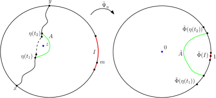
Figure B.1: An illustration of the proof of Lemma B.3. In the left figure, the domain $D_{\eta}$ is the part of $\mathbf{D}$ lying to the right of the curve $\eta$ (including the dashed part $\eta([t_{1},t_{2}])$) and the domain $D_{\eta}^{0}$ is the complement of the two solid black segments of $\eta$. The probability that a Brownian motion started from $z$ exits $D_{\eta}^{0}$ in the red arc $I$ is bounded by the supremum of the harmonic measure of $I$ in $D_{\eta}^{0}$ from any point of the green crosscut $A$. This, in turn, is bounded by a constant times the supremum of the harmonic measure of $I$ in $D_{\eta}$ from any point of $A$, which is bounded by the harmonic measure of $I$ from $z$ in $D_{\eta}$ by our choice of $\widetilde{A}$.

We now deduce a consequence of Lemma B.1 which allows us to compare the derivatives of conformal maps associated with an entire curve and with part of a curve. In particular, we consider a curve $\eta$ connecting two points of $\partial\mathbf{D}$ and compare the derivative behavior of a conformal map from the right side of $\mathbf{D}\setminus\eta$ to $\mathbf{D}$ and the derivative behavior of a conformal map from the complement of a segment of $\eta$ and its time reversal to $\mathbf{D}$.

Lemma B.3.

Fix $\delta>0$. Let $x,y\in\partial\mathbf{D}$ and $m\in(x,y)_{\partial\mathbf{D}}$ with $|x-m|,|y-m|\geq\delta$. Also let $\eta:[0,\infty]\rightarrow\mathbf{D}$ be a simple curve which does not intersect $(x,y)_{\partial\mathbf{D}}$ and let $D_{\eta}$ be the connected component of $\mathbf{D}\setminus\eta$ containing $[x,y]_{\partial\mathbf{D}}$ on its boundary. Let $\Psi_{\eta}:D_{\eta}\rightarrow\mathbf{D}$ be the conformal map taking $x$ to $-i$, $y$ to $i$, and $m$ to 1.

Fix $t_{2}>t_{1}\geq 0$, set $D_{\eta}^{0}=\mathbf{D}\setminus(\eta([0,t_{1}])\cup\eta([t_{2},\infty]))$, and let $\Phi:D_{\eta}^{0}\rightarrow\mathbf{D}$ be the conformal map taking $x^{+}$ to $-i$, $y^{-}$ to $i$, and $m$ to 1. Suppose that the following holds for some arc $I\subset[x,y]_{\partial\mathbf{D}}$ and some point $z\in D_{\eta}$.

1. $\operatorname{hm}^{z}(\eta([0,t_{1}]);D_{\eta})$ and $\operatorname{hm}^{z}(\eta([t_{2},\infty]);D_{\eta})$ are each at least $\delta$.

2. The length of $\Psi_{\eta}(I)$ and the distance from $\Psi_{\eta}(z)$ to $\Psi_{\eta}(I)$ are each at least $\delta$.

3. The length of $\Phi(I)$ and the distance from $\Phi(z)$ to $\Phi(I)$ are each at least $\delta$.

Then $|\Phi^{\prime}(z)|\asymp|\Psi_{\eta}^{\prime}(z)|$ and $\operatorname{dist}(z,\partial D_{\eta})\asymp\operatorname{dist}(z,\partial D_{\eta}^{0})$ with implicit constants depending only on $\delta$ and $z$ but uniform for $z$ in compact subsets of $\mathbf{D}$.

Proof.

See Figure B.1 for an illustration of the proof.

By Lemma B.1,

$$|\Phi^{\prime}(z)|\asymp\frac{\operatorname{hm}^{z}(I;D_{\eta}^{0})}{\operatorname{dist}(z,\partial D_{\eta}^{0})}\quad\operatorname{and}\quad|\Psi_{\eta}^{\prime}(z)|\asymp\frac{\operatorname{hm}^{z}(I;D_{\eta})}{\operatorname{dist}(z,\partial D_{\eta})}$$

with the implicit constants depending only on $\delta$. We clearly have $\operatorname{hm}^{z}(I;D_{\eta}^{0})\geq\operatorname{hm}^{z}(I;D_{\eta})$. By the Beurling estimate, if $r$ is chosen sufficiently large, in a manner depending only on $\delta$, then $\operatorname{hm}^{z}(\eta\cap B_{r\operatorname{dist}(z,\eta)}(z);D_{\eta})\geq 1-\delta/2$. So, our hypothesis 1 implies that $\operatorname{dist}(z,\partial D_{\eta})\asymp\operatorname{dist}(z,\partial D_{\eta}^{0})$. Therefore it is enough to prove

$$\operatorname{hm}^{z}(I;D_{\eta}^{0})\preceq\operatorname{hm}^{z}(I;D_{\eta})$$ (B.1)

with the implicit constant depending only on $\delta$.

Let $\widetilde{\Psi}_{\eta}:D_{\eta}\rightarrow\mathbf{D}$ be the conformal map taking $z$ to 0 and $m$ to 1. By conformal invariance of harmonic measure and our hypothesis 1, the distance from each of $\widetilde{\Psi}_{\eta}(\eta(t_{1}))$ and $\widetilde{\Psi}_{\eta}(\eta(t_{2}))$ to $\widetilde{\Psi}_{\eta}(I)$ is at least $2\pi\delta$. Hence we can choose a crosscut $\widetilde{A}$ in $\mathbf{D}$ which disconnects 0 from $\widetilde{\Psi}_{\eta}(I)$ such that each point of $\widetilde{A}$ lies at distance at least $\delta$ from $\widetilde{\Psi}_{\eta}(I)$ and from $[\widetilde{\Psi}_{\eta}(\eta(t_{2})),\widetilde{\Psi}_{\eta}(\eta(t_{t}))]_{\partial\mathbf{D}}$. The harmonic measure of $\widetilde{\Psi}_{\eta}(I)$ from each point of $\widetilde{A}$ in $\mathbf{D}$ is bounded above by a constant depending only on $\delta$ times the length of $\widetilde{\Psi}_{\eta}(I)$, which in turn is proportional to $\operatorname{hm}^{z}(I;D_{\eta})$. Furthermore, the harmonic measure of the arc $[\widetilde{\Psi}_{\eta}(\eta(t_{2})),\widetilde{\Psi}_{\eta}(\eta(t_{t}))]_{\partial\mathbf{D}}$ from each point of $\widetilde{A}$ in $\mathbf{D}$ is bounded above by a constant $a<1$ depending only on $\delta$.

Let $A=\widetilde{\Psi}_{\eta}^{-1}(\widetilde{A})$. Then

$$\operatorname{hm}^{w}(I;D_{\eta})\preceq\operatorname{hm}^{z}(I;D_{\eta}),\qquad\operatorname{hm}^{w}(\eta([t_{1},t_{2}]);D_{\eta})\leq a\qquad\forall w\in A$$ (B.2)

with the implicit constant depending only on $\delta$.

A Brownian motion started from $z$ must hit $A$ before exiting $D_{\eta}^{0}$ in $I$. Therefore,

$$\operatorname{hm}^{z}(I;D_{\eta}^{0})\leq\sup_{w\in A}\operatorname{hm}^{w}(I;D_{\eta}^{0}).$$ (B.3)

For $w\in A$, we can decompose the event that a Brownian motion $B$ started at $w$ exits $D_{\eta}^{0}$ in $I$ as the union of the event that $B$ hits $I$ before $\eta([t_{1},t_{2}])$ and the event that $B$ hits $\eta([t_{1},t_{2}])$ and then $I$. By (B.2) the former event has probability at most a constant $C$ (depending only on $\delta$) times $\operatorname{hm}^{z}(I;D_{\eta})$. By the Markov property the latter event has probability at most

$$\sup_{w\in A}\operatorname{hm}^{w}(\eta([t_{1},t_{2}]);D_{\eta})\sup_{v\in\eta([t_{1},t_{2}])}\operatorname{hm}^{v}(I;D_{\eta}^{0}).$$

Since $A$ disconnects $\eta([t_{1},t_{2}])$ from $I$ in $D_{\eta}^{0}$ we have $\sup_{v\in\eta([t_{1},t_{2}])}\operatorname{hm}^{v}(I;D_{\eta}^{0})\leq\sup_{w\in A}\operatorname{hm}^{w}(I;D_{\eta}^{0})$. By combining this with (B.2) we get

$$\sup_{w\in A}\operatorname{hm}^{w}(I;D_{\eta}^{0})\leq C\operatorname{hm}^{z}(I;D_{\eta})+a\sup_{w\in A}\operatorname{hm}^{w}(I;D_{\eta}^{0}).$$ (B.4)

Since $a<1$, we can re-arrange the estimate (B.4) to get

$$\sup_{w\in A}\operatorname{hm}^{w}(I;D_{\eta}^{0})\preceq\operatorname{hm}^{z}(I;D_{\eta}),$$

which together with (B.3) yields (B.1). ∎

Appendix C Strict mutual absolute continuity for SLE

Definition C.1.

We say that a measure $\mu$ is strictly mutually absolutely continuous (s.m.a.c.) with respect to a measure $\nu$ if $\mu$ and $\nu$ are mutually absolutely continuous with Radon-Nikodym derivative a.e. bounded above and below by finite and positive constants.

In this appendix we will prove a lemma which gives that the conditional law of the “middle part” of an $\operatorname{SLE}_{\kappa}(\rho^{L};\rho^{R})$ curve given the initial and terminal segments, on a certain regularity event, is s.m.a.c. with respect to the law of the middle part of an ordinary $\operatorname{SLE}_{\kappa}$ curve (see Lemma C.4 below for an exact statement). This result is needed in the proof of our two-point estimate (see in particular Lemma 7.3). We will deduce our desired result from [MW17, Lemma 2.8] (which gives a similar strict mutual absolute continuity statement for $\operatorname{SLE}_{\kappa}(\underline{\rho})$ curves in domains which agree in a neighborhood of the starting point) together with the coupling results of [MS16c], described in Section 2.5.

Before we can prove this result, we need to define the regularity event for the initial and terminal segments of the path which we will work on. Let $x,y\in\partial\mathbf{D}$ be distinct. Let $\eta$ be a random curve from $x$ to $y$ in $\mathbf{D}$, with time reversal $\overline{\eta}$. In what follows, we write $\mathcal{B}_{\beta}=B_{e^{-\beta}}(0)$ and let $\tau_{\beta}$ (resp. $\overline{\tau}_{\beta}$) be the first time $\eta$ (resp. $\overline{\eta}$) hits $\mathcal{B}_{\beta}$, as in Section 6.

Fix $\Delta>\Delta^{\prime}>\widetilde{\Delta}>0$. Suppose we are given times $\sigma,\overline{\sigma}>0$. Let $\eta^{*}$ be the part of $\eta$ between $\eta(\sigma)$ and $\overline{\eta}(\overline{\sigma})$. Let $H^{*}=H^{*}(\eta^{*};\widetilde{\Delta})$ be the event that $\eta^{*}\subset\mathcal{B}_{\widetilde{\Delta}}$. Let $S=S(\eta;\sigma,\overline{\sigma},\Delta,\widetilde{\Delta})$ be the event that the following occur.

1. $\tau_{\Delta}\leq\sigma<\infty$ and $\overline{\tau}_{\Delta}\leq\overline{\sigma}<\infty$ (here, $\tau_{\Delta}=\tau_{\beta}$ and $\overline{\tau}_{\Delta}=\overline{\tau}_{\beta}$ with $\beta=\Delta$).

2. $\eta^{\sigma}$ (resp. $\overline{\eta}^{\overline{\sigma}}$) is contained in the $e^{-2\Delta}$-neighborhood of the segment $[x,0]$ (resp. $[y,0]$).

3. The conditional probability of $H^{*}$ given $\eta^{\sigma}\cup\overline{\eta}^{\overline{\sigma}}$ is positive.

Also let $S^{*}=S^{*}(\eta;\sigma,\overline{\sigma},\Delta,\Delta^{\prime},\widetilde{\Delta})$ be the event that the following occur.

1. $S(\eta;\sigma,\overline{\sigma},\Delta,\widetilde{\Delta})$ occurs.

2. $\eta([\tau_{\Delta^{\prime}},\sigma])$ (resp. $\overline{\eta}([\overline{\tau}_{\Delta^{\prime}},\overline{\sigma}])$) is contained in $\mathcal{B}_{\widetilde{\Delta}}$.

Remark C.2.

If the event $L$ and the times $\sigma$ and $\overline{\sigma}$ are defined as in Section 7.2, then we have

$$L\subset S^{*}(\eta;\sigma,\overline{\sigma},\Delta,\Delta/2,\widetilde{\Delta}).$$

This is the primary reason for our interest in the event $S^{*}(\cdot)$.

Remark C.3.

In the case that $\eta$ is an $\operatorname{SLE}_{\kappa}(\rho^{L};\rho^{R})$ (which is what we consider in the section) one can show that condition 3 in the definition of $S$ is in fact implied by the other conditions in the definition of $S$. The idea to establish this is to realize $\eta$ as a flow line of a GFF, then condition on two counterflow lines (run up to a certain stopping time) with the property that the interface between them is a.s. equal to $\overline{\eta}^{\overline{\sigma}}$. See [MS16d, Section 5.4] for a similar argument. We do not need this fact here though, so for the sake of brevity we include condition 3 as a condition.

The main result of this section is the following.

Lemma C.4.

Let $\rho^{L},\rho^{R}\in(-2,0]$, $\delta>0$, and $x,y\in\partial\mathbf{D}$ with $|x-y|\geq\delta$. Let $\eta$ be a chordal $\operatorname{SLE}_{\kappa}(\rho^{L};\rho^{R})$ process from $x$ to $y$ in $\mathbf{D}$ with force points located at $x^{-}$ and $x^{+}$. Let $\overline{\eta}$ be its time reversal. Let $\sigma$ be a stopping time for $\eta$ and let $\overline{\sigma}$ be a stopping time for the filtration generated by $\eta^{\sigma}$ and $\overline{\eta}$. Let $S^{*}=S^{*}(\eta;\sigma,\overline{\sigma},\Delta,\Delta^{\prime},\widetilde{\Delta})$ as above. Also let $\eta^{*}$ and $H^{*}=H^{*}(\eta^{*};\widetilde{\Delta})$ be as above. Let $D$ be the connected component of $\mathbf{D}\setminus(\eta^{\sigma}\cup\overline{\eta}^{\overline{\sigma}})$ containing 0.

If $\widetilde{\Delta}$ (and hence also $\Delta^{\prime}$ and $\Delta$) is chosen sufficiently large, in a manner depending only on $\delta$, $\rho^{L}$, and $\rho^{R}$, then a.s. on $S^{*}$ the regular conditional law of $\eta^{*}$ given $\eta^{\sigma}\cup\overline{\eta}^{\overline{\sigma}}$ and the event $H^{*}$ is s.m.a.c. with respect to the law of a chordal $\operatorname{SLE}_{\kappa}$ from $\eta(\sigma)$ to $\overline{\eta}(\overline{\sigma})$ in $D$ conditioned on $H^{*}$, with deterministic constants depending only on $\rho^{L},\rho^{R},\kappa,\Delta,\Delta^{\prime},$ $\widetilde{\Delta}$, and $\delta$.

The idea of the proof of Lemma C.4 is to consider a GFF on $\mathbf{D}$ whose flow line $\eta_{0}$ is an ordinary SLE_κ, then grow auxiliary flow lines with the same start and endpoints in such a way that the conditional law of $\eta_{0}$ given these auxiliary flow lines is that of an SLE${}_{\kappa}(\rho^{L};\rho^{R})$ for the given values of $\rho^{L}$ and $\rho^{R}$. By [MW17, Lemma 2.8], the conditional laws of these auxiliary flow lines given $\eta_{0}$ do not depend strongly on a small segment in the middle of $\eta_{0}$. We then apply Bayes’ rule to invert the conditioning. See Figure C.1 for an illustration of the argument.

For the proof of Lemma C.4, we will assume neither $\rho^{L}$ nor $\rho^{R}$ is equal to 0; the case when one of the force points is equal to 0 is treated similarly but with only a single auxiliary flow line.

Choose $\Delta_{0}>\widetilde{\Delta}_{0}>0$ satisfying $\widetilde{\Delta}_{0}<\widetilde{\Delta}<\Delta^{\prime}<\Delta_{0}<\Delta$, with $\Delta,\Delta^{\prime},$ and $\widetilde{\Delta}$ as in the statement of Lemma C.4. Let $\eta_{0}$ be an ordinary chordal $\operatorname{SLE}_{\kappa}$ from $x$ to $y$ in $\mathbf{D}$. Let $\overline{\eta}_{0}$ be the time reversal of $\eta_{0}$. Let $\sigma_{0}$ (resp. $\overline{\sigma}_{0}$) be the first time $\eta_{0}$ (resp. $\overline{\eta}_{0}$) hits $\mathcal{B}_{\widetilde{\Delta}}$. Let $\eta_{0}^{*}$ be the part of $\eta_{0}$ between $\eta(\sigma_{0})$ and $\overline{\eta}(\overline{\sigma}_{0})$. Also let

$$S_{0}:=S(\eta_{0};\sigma_{0},\overline{\sigma}_{0},\Delta_{0},\widetilde{\Delta}_{0}),\qquad H^{*}_{0}=H^{*}(\eta^{*}_{0};\widetilde{\Delta}_{0}).$$ (C.1)

We can couple $\eta_{0}$ with a GFF $h$ on $\mathbf{D}$ with appropriately chosen boundary data in such a way that $\eta_{0}$ is the zero angle flow line (in the sense of Section 2.5) of $h$ started from $x$. Let $\theta^{L}>0$ and $\theta^{R}<0$ be chosen so that

$$\frac{\theta^{L}\chi}{\lambda}-2=\rho^{L},\qquad-\frac{\theta^{R}\chi}{\lambda}-2=\rho^{R}.$$ (C.2)

Let $\eta_{-}$ and $\eta_{+}$ be the flow lines of $h$ started from $x$ with angles $\theta^{L}$ and $\theta^{R}$, respectively. Since $\rho^{L},\rho^{R}\in(-2,0)$, the flow lines $\eta_{-}$ and $\eta_{+}$ are well defined. Let $D_{0}$ be the connected component of $\mathbf{D}\setminus(\eta_{-}\cup\eta_{+})$ containing the origin. Let $b$ and $\overline{b}$, respectively, be the first and last point on $\partial D_{0}$ hit by $\eta_{0}$. By the results of [MS16c, Section 7], the conditional law of the part of $\eta_{0}$ which lies in $D_{0}$ given $\eta_{-}\cup\eta_{+}$ is that of a chordal $\operatorname{SLE}_{\kappa}(\rho^{L};\rho^{R})$ from $b$ to $\overline{b}$ in $D_{0}$ with force points located on either side of $b$.

We also fix a small parameter $\alpha\in(0,1)$ and let $t_{-}$ and $t_{+}$ respectively be the first times $\eta_{-}$ and $\eta_{+}$ exit $B_{1-\alpha}(0)$.

Throughout the remainder of this subsection, we require all implicit constants, including those in s.m.a.c., to depend only on $\Delta,\widetilde{\Delta},\Delta^{\prime},\Delta_{0},\widetilde{\Delta}_{0},\alpha,\rho^{L},\rho^{R},\kappa$, and $\delta$ (in particular, implicit constants are not allowed to depend on the realization of whatever we are conditioning on or on the choice of stopping times $\sigma,\overline{\sigma}$).

Lemma C.5.

Let $\omega_{0}$ be a realization of $\eta_{0}^{\sigma_{0}}\cup\overline{\eta}^{\overline{\sigma}_{0}}$ for which $S_{0}$ occurs. If $\widetilde{\Delta}_{0}$ (and hence also $\Delta_{0}$) is chosen sufficiently large and $\alpha>0$ is chosen sufficiently small, in a manner which is uniform over values of the endpoints $x$ and $y$ such that $|x-y|$ is bounded below, then the following is true for a.e. such $\omega_{0}$. Almost surely, the conditional law of $\eta^{*}_{0}$ given $\{\eta_{0}^{\sigma_{0}}\cup\overline{\eta}^{\overline{\sigma}_{0}}=\omega_{0}\}$, $H_{0}^{*}$, and $(\eta_{-}^{t_{-}},\eta_{+}^{t_{+}})$ is s.m.a.c. with respect to the conditional law of $\eta^{*}_{0}$ given only $\{\eta_{0}^{\sigma_{0}}\cup\overline{\eta}^{\overline{\sigma}_{0}}=\omega_{0}\}$ and $H_{0}^{*}$.

Proof.

Let $\mathbf{P}_{\omega_{0}}$ denote the regular conditional probability given $\{\eta_{0}^{\sigma_{0}}\cup\overline{\eta}^{\overline{\sigma}_{0}}=\omega_{0}\}$ and the event $H_{0}^{*}$. Let $A^{*}_{0}$ be an event with positive $\mathbf{P}_{\omega_{0}}$-probability which is determined by $\eta_{0}^{*}$ and $\eta_{0}^{\sigma_{0}}\cup\overline{\eta}^{\overline{\sigma}_{0}}$ and is contained in $H^{*}_{0}$. Let $A^{F}_{0}$ be the intersection of $H_{0}^{*}$ with an event which is determined by $\eta_{0}^{\sigma_{0}}\cup\overline{\eta}_{0}^{\overline{\sigma}_{0}}$ and $(\eta_{-}^{t_{-}},\eta_{+}^{t_{+}})$ and contained in $S_{0}$ which also satisfies $\mathbf{P}_{\omega_{0}}(A_{0}^{F})>0$. By Bayes’ rule,

$$\mathbf{P}_{\omega_{0}}(A^{*}_{0}\,|\,A^{F}_{0})=\frac{\mathbf{P}_{\omega_{0}}(A^{F}_{0}\,|\,A^{*}_{0})\mathbf{P}_{\omega_{0}}(A^{*}_{0})}{\mathbf{P}_{\omega_{0}}(A^{F}_{0})}.$$ (C.3)

Hence we are lead to study the conditional law of $(\eta_{-}^{t_{-}},\eta_{+}^{t_{+}})$ given $\{\eta_{0}^{\sigma_{0}}\cup\overline{\eta}^{\overline{\sigma}_{0}}=\omega_{0}\}$ and $\eta_{0}^{*}$, for varying realizations of $\eta^{*}_{0}$ for which $H^{*}_{0}$ occurs.

By the results of [MS16c, Section 7.1], the conditional law of $\eta_{+}$ given $\eta_{0}$ is that of a chordal $\operatorname{SLE}_{\kappa}(\rho^{L}_{F};\rho^{R}_{F})$ process from $x$ to $y$ in the right connected component of $\mathbf{D}\setminus\eta_{0}$ for certain $\rho^{L}_{F},\rho^{R}_{F}>-2$ depending on $\rho^{L}$ and $\rho^{R}$. A similar statement holds for $\eta_{-}$. Furthermore, $\eta_{+}$ and $\eta_{-}$ are conditionally independent given $\eta_{0}$. By [MW17, Lemma 2.8] and the analog of condition 2 in the definition of $S_{0}$, if $\widetilde{\Delta}_{0}$ is chosen sufficiently large and $\alpha>0$ is chosen sufficiently small then the conditional laws of the pair $(\eta_{-}^{t_{-}},\eta_{+}^{t_{+}})$ given $\{\eta_{0}^{\sigma_{0}}\cup\overline{\eta}^{\overline{\sigma}_{0}}=\omega_{0}\}$ and $\eta^{*}_{0}$ for varying realizations of $\eta^{*}_{0}$ for which $H_{0}^{*}$ occurs are all s.m.a.c.. By averaging over all such realizations, we get $\mathbf{P}_{\omega_{0}}(A^{F}_{0}\,|\,A^{*}_{0})\asymp\mathbf{P}_{\omega_{0}}(A^{F}_{0})$. By (C.3) we therefore have $\mathbf{P}_{\omega_{0}}(A^{*}_{0}\,|\,A^{F}_{0})\asymp\mathbf{P}_{\omega_{0}}(A^{*}_{0})$. ∎

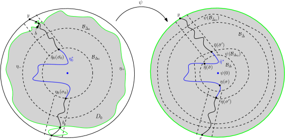
Figure C.1: An illustration of the setup for the proof of Lemma C.4. The curve $\eta_{0}$ in the left picture has the law of an ordinary chordal $\operatorname{SLE}_{\kappa}$ from $x$ to $y$ in $\mathbf{D}$. The curve $\eta$ in the right picture (obtained by mapping the “pocket” $D_{0}$ formed green auxiliary flow lines to $\mathbf{D}$) has the law of a chordal $\operatorname{SLE}_{\kappa}(\rho^{L};\rho^{R})$ from $x$ to $y$. The amount by which $\psi$ distorts distances is exaggerated for clarity— typically, $\psi$ is close to the identity on the event $F$.

Proof of Lemma C.4.

Let $D_{0}$, $b$, and $\overline{b}$ be defined as in the discussion just above Lemma C.5. Let $\psi:D_{0}\rightarrow\mathbf{D}$ be the conformal map which takes $b$ to $x$ and $\overline{b}$ to $y$, chosen so that $|\psi(0)|$ is minimal amongst all such maps, and let

$$\eta:=\psi(\eta_{0}\cap D_{0}),\qquad\widetilde{\eta}^{*}:=\psi(\eta_{0}^{*}).$$

Also let $\overline{\eta}$ be the time reversal of $\eta$. We define the objects in the statement of the lemma with this choice of $\eta$. By the discussion just above Lemma C.5, the conditional law of $\eta$ given $\eta_{-}$ and $\eta_{+}$ is that of a chordal $\operatorname{SLE}_{\kappa}(\rho^{L};\rho^{R})$ process from $x$ to $y$ in $\mathbf{D}$.

Fix $\epsilon>0$, to be chosen later, and let $F=F(\epsilon)$ be the event that the following occur.

1. $\eta_{-}$ and $\eta_{+}$ trace all of $\partial D_{0}$ before times $t_{-}$ and $t_{+}$ (equivalently, since $\eta_{\pm}$ cannot cross themselves or each other, $t_{-}=t_{+}=\infty$).

2. $|\psi(z)-z|\leq\epsilon$ for each $z\in D_{0}$.

By Lemma 2.17, for each $\epsilon>0$ a.s. $\mathbf{P}(F\,|\,\eta_{0})>0$.

By choosing $\epsilon>0$ sufficiently small (depending only on $\Delta,\Delta^{\prime},\widetilde{\Delta},\Delta_{0}$, and $\widetilde{\Delta}_{0}$), we can arrange that the following are true on $F$.

1. $\mathcal{B}_{\Delta}\subset\psi(\mathcal{B}_{\Delta_{0}})\subset\psi(\mathcal{B}_{\Delta^{\prime}})\subset\psi(\mathcal{B}_{\widetilde{\Delta}_{0}})\subset\mathcal{B}_{\widetilde{\Delta}}$.

2. The image under $\psi$ of the $e^{-2\Delta_{0}}$-neighborhood of the segment $[x,0]$ (resp. $[y,0]$) contains the $e^{-2\Delta}$-neighborhood of the segment $[x,0]$ (resp. $[y,0]$).

On the event $F$, let $\sigma^{\prime}$ and $\overline{\sigma}^{\prime}$ be the stopping times for $\eta$ and $\overline{\eta}$ corresponding to $\sigma_{0}$ and $\overline{\sigma}_{0}$, so $\psi(\eta_{0}(\sigma_{0}))=\eta(\sigma^{\prime})$, $\psi(\overline{\eta}_{0}(\overline{\sigma}_{0}))=\overline{\eta}(\overline{\sigma}^{\prime})$, and $\widetilde{\eta}^{*}$ is the part of $\eta$ between $\eta(\sigma^{\prime})$ and $\overline{\eta}(\overline{\sigma}^{\prime})$. Also let $\eta^{*}$ be the part of $\eta$ between $\sigma$ and $\overline{\sigma}$, as in the statement of the lemma.

By conditions 1 and 2 above together with condition 2 in the definition of $S^{*}$,

$$F\cap S^{*}\cap H^{*}\subset F\cap S_{0}\cap H^{*}_{0}.$$ (C.4)

(Note that the first inclusion is the only place where we use condition 2 in the definition of $S^{*}$.) Furthermore, by the first inclusion in condition 1 and condition 1 in the definition of $S$, on $F\cap S$ a.s.

$$\sigma^{\prime}\leq\tau_{\Delta}\leq\sigma\quad\operatorname{and}\quad\overline{\sigma}^{\prime}\leq\overline{\tau}_{\Delta}\leq\overline{\sigma}.$$ (C.5)

Now let $(\omega_{0},\omega_{F})$ be a realization of $\left(\eta_{0}^{\sigma_{0}}\cup\overline{\eta}_{0}^{\overline{\sigma}_{0}},\eta_{+}^{t_{+}}\cup\eta_{-}^{t_{-}}\right)$ for which $F\cap S_{0}$ occurs. We observe the following.

1. By the strong Markov property and reversibility of ordinary SLE_κ, the conditional law of $\eta_{0}^{*}$ given $\{\eta_{0}^{\sigma_{0}}\cup\overline{\eta}_{0}^{\overline{\sigma}_{0}}=\omega_{0}\}$ and $H_{0}^{*}$ is that of a chordal $\operatorname{SLE}_{\kappa}$ from $\eta_{0}(\sigma_{0})$ to $\overline{\eta}_{0}(\overline{\sigma}_{0})$ in $\mathbf{D}\setminus(\eta_{0}^{\sigma_{0}}\cup\overline{\eta}_{0}^{\overline{\sigma}_{0}})$, conditioned on $H_{0}^{*}$.

2. It therefore follows from Lemma C.5 that the conditional law of $\eta^{*}_{0}$ given $\{\left(\eta_{0}^{\sigma_{0}}\cup\overline{\eta}_{0}^{\overline{\sigma}_{0}},\eta_{+}^{t_{+}}\cup\eta_{-}^{t_{-}}\right)=(\omega_{0},\omega_{F})\}$ and $H_{0}^{*}$ is a.s. s.m.a.c. with respect to the law of a chordal $\operatorname{SLE}_{\kappa}$ from $\eta_{0}(\sigma_{0})$ to $\overline{\eta}_{0}(\overline{\sigma}_{0})$ in $\mathbf{D}\setminus(\eta_{0}^{\sigma_{0}}\cup\overline{\eta}_{0}^{\overline{\sigma}_{0}})$, conditioned on $H_{0}^{*}$.

3. By [MW17, Lemma 2.8], this latter law is s.m.a.c. with respect to the law of a chordal $\operatorname{SLE}_{\kappa}$ from $\eta_{0}(\sigma_{0})$ to $\overline{\eta}_{0}(\overline{\sigma}_{0})$ in the connected component of $D_{0}\setminus(\eta_{0}^{\sigma_{0}}\cup\overline{\eta}_{0}^{\overline{\sigma}_{0}})$ containing 0, conditioned on $H^{*}_{0}$.

4. Therefore, the conditional law of $\widetilde{\eta}^{*}$ given $\{\left(\eta_{0}^{\sigma_{0}}\cup\overline{\eta}_{0}^{\overline{\sigma}_{0}},\eta_{+}^{t_{+}}\cup\eta_{-}^{t_{-}}\right)=(\omega_{0},\omega_{F})\}$ and $H^{*}_{0}$ is s.m.a.c. with respect to the law of a chordal $\operatorname{SLE}_{\kappa}$ from $\eta(\sigma^{\prime})$ to $\overline{\eta}(\overline{\sigma}^{\prime})$ in the component of $\mathbf{D}\setminus(\eta^{\sigma^{\prime}}\cup\overline{\eta}^{\overline{\sigma}^{\prime}})$ containing 0, conditioned on $H_{0}^{*}$.

5. By (C.4), (C.5), and the Markov property and reversibility of ordinary $\operatorname{SLE}_{\kappa}$, assertion 4 implies that the conditional law of $\eta^{*}$ given $\{\eta_{+}^{t_{+}}\cup\eta_{-}^{t_{-}}=\omega_{F}\}$; a realization of $\eta^{\sigma}\cup\overline{\eta}^{\overline{\sigma}}$ for which $S^{*}$ occurs; and $H^{*}$ is a.s. s.m.a.c. with respect to the law of a chordal $\operatorname{SLE}_{\kappa}$ from $\eta(\sigma^{\prime})$ to $\overline{\eta}(\overline{\sigma}^{\prime})$ in the component of $\mathbf{D}\setminus(\eta^{\sigma^{\prime}}\cup\overline{\eta}^{\overline{\sigma}^{\prime}})$ containing 0, conditioned on $H^{*}$.

Since the law of $\eta$ given a.e. $\omega_{F}$ is that of a chordal $\operatorname{SLE}_{\kappa}(\rho^{L};\rho^{R})$ from $x$ to $y$ in $\mathbf{D}$ and there is a positive probability event of choices for $\omega_{F}$, assertion 5 implies the statement of the lemma. ∎

References

- [ABJ15] T. Alberts, I. Binder, and F. Johansson Viklund. A Dimension Spectrum for SLE Boundary Collisions. ArXiv e-prints, January 2015, 1501.06212.
- [BD14] I. Binder and B. Duplantier. Private communication, 2014.
- [Bef08] V. Beffara. The dimension of the SLE curves. Ann. Probab., 36(4):1421–1452, 2008, math/0211322. MR2435854 (2009e:60026)
- [BS05] D. Beliaev and S. Smirnov. Harmonic measure on fractal sets. In European Congress of Mathematics, pages 41–59. Eur. Math. Soc., Zürich, 2005. MR2185735 (2007d:31013)
- [BS09] D. Beliaev and S. Smirnov. Harmonic measure and SLE. Comm. Math. Phys., 290(2):577–595, 2009, 0801.1792. MR2525631 (2011c:60265)
- [DB02] B. Duplantier and I. Binder. Harmonic measure and winding of conformally invariant curves. Physical Review Letters, 89(264101), 2002, cond-mat/0208045.
- [DB08] B. Duplantier and I. Binder. Harmonic measure and winding of random conformal paths: A Coulomb gas perspective. Nucl.Phys. B, 802:494–513, 2008, 0802.2280.
- [DHBZ15] B. Duplantier, X. Hieu Ho, T. Binh Le, and M. Zinsmeister. Logarithmic Coefficients and Multifractality of Whole-Plane SLE. ArXiv e-prints, April 2015, 1504.05570.
- [DMS14] B. Duplantier, J. Miller, and S. Sheffield. Liouville quantum gravity as a mating of trees. ArXiv e-prints, September 2014, 1409.7055.
- [DNNZ12] B. Duplantier, C. Nguyen, N. Nguyen, and M. Zinsmeister. The Coefficient Problem and Multifractality of Whole-Plane SLE and LLE. ArXiv e-prints, November 2012, 1211.2451.
- [DS11] B. Duplantier and S. Sheffield. Liouville quantum gravity and KPZ. Invent. Math., 185(2):333–393, 2011, 1206.0212. MR2819163 (2012f:81251)
- [Dub09a] J. Dubédat. Duality of Schramm-Loewner evolutions. Ann. Sci. Éc. Norm. Supér. (4), 42(5):697–724, 2009, 0711.1884. MR2571956 (2011g:60151)
- [Dub09b] J. Dubédat. SLE and the free field: partition functions and couplings. J. Amer. Math. Soc., 22(4):995–1054, 2009, 0712.3018. MR2525778 (2011d:60242)
- [Dup99a] B. Duplantier. Harmonic Measure Exponents for Two-Dimensional Percolation. Physical Review Letters, 82(3940), 1999, cond-mat/9901008.
- [Dup99b] B. Duplantier. Two-Dimensional Copolymers and Exact Conformal Multifractality. Physical Review Letters, 82(880), 1999, cond-mat/9812439.
- [Dup00] B. Duplantier. Conformally invariant fractals and potential theory. Physical Review Letters, 84(7):1363–1367, 2000, cond-mat/9908314.
- [Dup03] B. Duplantier. Higher conformal multifractality. Journal of Statistical Physics, 110(3–6):691–738, 2003, cond-mat/0207743.
- [Dup04] B. Duplantier. Conformal fractal geometry and boundary quantum gravity. In Fractal Geometry and Applications: a Jubilee of Benôit Mandelbrot, Part 2, Proc. Sympos. Pure Math., 72, pages 365––482, Providence, RI, 2004. Amer. Math. Soc., math-ph/0303034.
- [HMP10] X. Hu, J. Miller, and Y. Peres. Thick points of the Gaussian free field. Ann. Probab., 38(2):896–926, 2010, 0902.3842. MR2642894 (2011c:60117)
- [HS08] H. Hedenmalm and A. Sola. Spectral notions for conformal maps: a survey. Comput. Methods Funct. Theory, 8(1-2):447–474, 2008. MR2419488 (2009f:30002)
- [JVL11] F. Johansson Viklund and G. F. Lawler. Optimal Hölder exponent for the SLE path. Duke Math. J., 159(3):351–383, 2011, 0904.1180. MR2831873
- [JVL12] F. Johansson Viklund and G. F. Lawler. Almost sure multifractal spectrum for the tip of an SLE curve. Acta Math., 209(2):265–322, 2012, 0911.3983. MR3001607
- [Kra96] P. Kraetzer. Experimental bounds for the universal integral means spectrum of conformal maps. Complex Variables Theory Appl., 31(4):305–309, 1996. MR1427159 (97m:30018)
- [Law96] G. Lawler. The dimension of the frontier of planar Brownian motion. Electron. Comm. Probab., 1:no. 5, 29–47 (electronic), 1996. MR1386292 (97g:60110)
- [Law05] G. F. Lawler. Conformally invariant processes in the plane, volume 114 of Mathematical Surveys and Monographs. American Mathematical Society, Providence, RI, 2005. MR2129588 (2006i:60003)
- [Law09] G. F. Lawler. Multifractal analysis of the reverse flow for the Schramm-Loewner evolution. In Fractal geometry and stochastics IV, volume 61 of Progr. Probab., pages 73–107. Birkhäuser Verlag, Basel, 2009. MR2762674 (2012e:60209)
- [Lin08] J. R. Lind. Hölder regularity of the SLE trace. Trans. Amer. Math. Soc., 360(7):3557–3578, 2008. MR2386236 (2009f:60048)
- [LSW01a] G. F. Lawler, O. Schramm, and W. Werner. The dimension of the planar Brownian frontier is . Math. Res. Lett., 8(4):401–411, 2001, math/0010165. MR1849257 (2003a:60127b)
- [LSW01b] G. F. Lawler, O. Schramm, and W. Werner. Values of Brownian intersection exponents. I. Half-plane exponents. Acta Math., 187(2):237–273, 2001, math/0003156. MR1879850 (2002m:60159a)
- [LSW01c] G. F. Lawler, O. Schramm, and W. Werner. Values of Brownian intersection exponents. II. Plane exponents. Acta Math., 187(2):275–308, 2001, math/9911084. MR1879851 (2002m:60159b)
- [LSW02] G. F. Lawler, O. Schramm, and W. Werner. Values of Brownian intersection exponents. III. Two-sided exponents. Ann. Inst. H. Poincaré Probab. Statist., 38(1):109–123, 2002. MR1899232 (2003d:60163)
- [LSW03] G. Lawler, O. Schramm, and W. Werner. Conformal restriction: the chordal case. J. Amer. Math. Soc., 16(4):917–955 (electronic), 2003, math/0209343v2. MR1992830 (2004g:60130)
- [LSW04] G. F. Lawler, O. Schramm, and W. Werner. Conformal invariance of planar loop-erased random walks and uniform spanning trees. Ann. Probab., 32(1B):939–995, 2004, math/0112234. MR2044671 (2005f:82043)
- [LY13] I. Loutsenko and O. Yermolayeva. Average harmonic spectrum of the whole-plane SLE. J. Stat. Mech. Theory Exp., (4):P04007, 17, 2013, 1203.2756. MR3077814
- [LY14] I. Loutsenko and O. Yermolayeva. New exact results in spectra of stochastic Loewner evolution. J. Phys. A, 47(16):165202, 15, 2014. MR3191679
- [Mak98] N. G. Makarov. Fine structure of harmonic measure. Algebra i Analiz, 10(2):1–62, 1998. MR1629379 (2000g:30018)
- [Mil10] J. Miller. Universality for SLE(4). ArXiv e-prints, October 2010, 1010.1356.
- [Mil16] J. Miller. Dimension of the SLE light cone, the SLE fan, and SLE for and . ArXiv e-prints, June 2016, 1606.07055.
- [MP10] P. Mörters and Y. Peres. Brownian motion. Cambridge Series in Statistical and Probabilistic Mathematics. Cambridge University Press, Cambridge, 2010. With an appendix by Oded Schramm and Wendelin Werner. MR2604525 (2011i:60152)
- [MS13] J. Miller and S. Sheffield. Imaginary geometry IV: interior rays, whole-plane reversibility, and space-filling trees. Probab. Theory Related Fields, to appear, 2013, 1302.4738.
- [MS16a] J. Miller and S. Sheffield. Gaussian free field light cones and SLE. ArXiv e-prints, June 2016, 1606.02260.
- [MS16b] J. Miller and S. Sheffield. Imaginary geometry III: reversibility of SLEκ for . Annals of Mathematics, 184(2):455–486, 2016, 1201.1498.
- [MS16c] J. Miller and S. Sheffield. Imaginary geometry I: interacting SLEs. Probab. Theory Related Fields, 164(3-4):553–705, 2016, 1201.1496. MR3477777
- [MS16d] J. Miller and S. Sheffield. Imaginary geometry II: Reversibility of for . Ann. Probab., 44(3):1647–1722, 2016, 1201.1497. MR3502592
- [MS16e] J. Miller and S. Sheffield. Quantum Loewner evolution. Duke Math. J., 165(17):3241–3378, 2016, 1312.5745. MR3572845
- [MSW14] J. Miller, N. Sun, and D. B. Wilson. The Hausdorff dimension of the CLE gasket. Ann. Probab., 42(4):1644–1665, 2014, 1403.6076. MR3262488
- [MSW16] J. Miller, S. Sheffield, and W. Werner. CLE Percolations. ArXiv e-prints, February 2016, 1602.03884.
- [MW17] J. Miller and H. Wu. Intersections of SLE Paths: the double and cut point dimension of SLE. Probab. Theory Related Fields, 167(1-2):45–105, 2017, 1303.4725. MR3602842
- [MWW15] J. Miller, S. S. Watson, and D. B. Wilson. The conformal loop ensemble nesting field. Probab. Theory Related Fields, 163(3-4):769–801, 2015, 1401.0217. MR3418755
- [Pom92] C. Pommerenke. Boundary behaviour of conformal maps, volume 299 of Grundlehren der Mathematischen Wissenschaften [Fundamental Principles of Mathematical Sciences]. Springer-Verlag, Berlin, 1992. MR1217706 (95b:30008)
- [Pom97] C. Pommerenke. The integral means spectrum of univalent functions. Zap. Nauchn. Sem. S.-Peterburg. Otdel. Mat. Inst. Steklov. (POMI), 237(Anal. Teor. Chisel i Teor. Funkts. 14):119–128, 229, 1997. MR1691287 (2000e:30031)
- [RS05] S. Rohde and O. Schramm. Basic properties of SLE. Ann. of Math. (2), 161(2):883–924, 2005, math/0106036. MR2153402 (2006f:60093)
- [Sch00] O. Schramm. Scaling limits of loop-erased random walks and uniform spanning trees. Israel J. Math., 118:221–288, 2000, math/9904022. MR1776084 (2001m:60227)
- [She05] S. Sheffield. Local sets of the gaussian free field: slides and audio. www.fields.utoronto.ca/audio/05-06/percolationSLE/sheffield1,www.fields.utoronto.ca/audio/05-81, 06/percolationSLE/sheffield2, www.fields.utoronto.ca/audio/05-06/percolationSLE/sheffield3, 2005.
- [She07] S. Sheffield. Gaussian free fields for mathematicians. Probab. Theory Related Fields, 139(3-4):521–541, 2007, math/0312099. MR2322706 (2008d:60120)
- [She16] S. Sheffield. Conformal weldings of random surfaces: SLE and the quantum gravity zipper. Ann. Probab., 44(5):3474–3545, 2016, 1012.4797. MR3551203
- [Smi10] S. Smirnov. Conformal invariance in random cluster models. I. Holomorphic fermions in the Ising model. Ann. of Math. (2), 172(2):1435–1467, 2010, 0708.0039. MR2680496 (2011m:60302)
- [SS05] O. Schramm and S. Sheffield. Harmonic explorer and its convergence to . Ann. Probab., 33(6):2127–2148, 2005, math/0310210. MR2184093 (2006i:60013)
- [SS09] O. Schramm and S. Sheffield. Contour lines of the two-dimensional discrete Gaussian free field. Acta Math., 202(1):21–137, 2009, math/0605337. MR2486487 (2010f:60238)
- [SS13] O. Schramm and S. Sheffield. A contour line of the continuum Gaussian free field. Probab. Theory Related Fields, 157(1-2):47–80, 2013, math/0605337. MR3101840
- [SW05] O. Schramm and D. B. Wilson. SLE coordinate changes. New York J. Math., 11:659–669 (electronic), 2005, math/0505368. MR2188260 (2007e:82019)
- [Wer04] W. Werner. Random planar curves and Schramm-Loewner evolutions. In Lectures on probability theory and statistics, volume 1840 of Lecture Notes in Math., pages 107–195. Springer, Berlin, 2004, math/030335. MR2079672 (2005m:60020)
- [WW14] M. Wang and H. Wu. Level Lines of Gaussian Free Field I: Zero-Boundary GFF. ArXiv e-prints, December 2014, 1412.3839.
- [Zha08a] D. Zhan. Duality of chordal SLE. Invent. Math., 174(2):309–353, 2008, 0712.0332. MR2439609 (2010f:60239)
- [Zha08b] D. Zhan. Reversibility of chordal SLE. Ann. Probab., 36(4):1472–1494, 2008. MR2435856 (2010a:60284)
- [Zha10] D. Zhan. Duality of chordal SLE, II. Ann. Inst. Henri Poincaré Probab. Stat., 46(3):740–759, 2010, 0803.2223. MR2682265 (2011i:60155)