TRANSPORT IN TWO–DIMENSIONAL QUANTUM WIRES WITH POINT SCATTERERS. THE WIGNER–SMITH TIME DELAY

Abstract

Electronic transport properties of the disordered quantum wires are considered. The disorder is introduced via impurities (point scatterers), distributed uniformly over the two-dimensional strip, which represents a model quantum wire. Incident electrons with a given energy are scattered on impurities and boundaries of the wire. The electron-electron interaction is neglected in the model. In particular, the intermediate regime and the localization regime of transport are studied in more detail in terms of the conductance and statistical properties of $S$-matrix ensemble for a given incident electron energy. The Wigner-Smith time delay distribution obtained for the localization regime is compared with the prediction for the scattering by a one-dimensional random potential.

I INTRODUCTION

Quantum transport through disordered mesoscopic systems and its description by the Random Matrix Theory (RMT) have been subject of an intense research for some time B97 . The phenomenon of quantum scattering is universal — it is also encountered in other physical systems, like for example in scattering of electromagnetic radiation by reflecting obstacles.

In order to study properties of the quantum transport, a two-dimensional model of the disordered wire is considered. The model, in which a number of point scatterers is randomly distributed over a strip, is continuous and yet solvable — expressions for scattering matrix (the $S$-matrix) elements can be given explicitly EGST96 .

Therefore, by means of varying the number of point scatterers together with the length of the sample, it is possible to modify properties of the electron transport through the wire in a well controlled way. Hence one can observe various types of the system behaviour ranging from the ballistic type of transport through “diffusive-like” scattering to the localization for a given energy of incoming electrons JP95 ; GSZZ98 . The model allows to study both macroscopic transport properties, like conductance, and microscopic signatures of the scattering processes such as eigenphase, $S$-matrix elements’ statistics and time delay distributions.

The aim of this contribution is to identify and investigate various regimes of the transport in the model quantum wire. The results will be compared with predictions of the standard Random Matrix Theory of transport. The signatures of various regimes of transport in the presence of the Time Reversal Symmetry will be considered in order to reveal regimes of the universal behaviour of the model and also deviations from that behaviour.

II THE MODEL

A disordered quantum wire is modelled with a two-dimensional rectangular strip of length $L$ and width $W$ ($W=\pi$ is taken) with hard walls EGST96 ; GSZZ98 . There is a finite number, $N$, of point scatterers randomly and uniformly distributed over the scattering region with coordinates $(x_{j},y_{j})$:

$$(x_{j},y_{j})\in(-L/2,L/2)\times(0,\pi),\qquad{\rm for}\qquad j=1,\ldots,N$$ (1)

An electron can enter the strip either from the left or from the right side. The number of channels, $M$, in the model wire is equal to the integer part of length of the wavevector $\bf{k}$ of the incoming electron. The scattering in the strip on impurities and boundaries is assumed to be elastic and the electron–electron interaction interaction is neglected. The hard wall boundary condition means that the wavefunction vanishes on the boundaries for all $x$:

$$\psi(x,0)=\psi(x,W)=0.$$ (2)

Figure (1) illustrates considered theoretical model of the quantum wire.

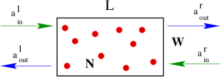
Figure 1: This illustrates a two-dimensional strip model of a quantum wire with $N$ point scatterers. The length of the strip is $L$ and the width is $W$ It has been taken $W=\pi$ in order to have the number of open channels $M=[k]$ (integer part of the incident electrons’ wavenumber $k$; the electrons’ energy $E=k^{2}$ in applied units here).

The scattering matrix $S$ relates incoming waves, denoted by $M$-component vectors $\bf{a}^{l}_{\rm{in}}$, $\bf{a}^{r}_{\rm{in}}$ (incoming waves respectively from the left and right side – see Figure (1)), with the outgoing waves $\bf{a}^{l}_{\rm{out}}$, $\bf{a}^{r}_{\rm{out}}$ in the following way:

$$\{\bf{a}^{l}_{\rm{out}},\bf{a}^{r}_{\rm{out}}\}=S\{\bf{a}^{l}_{\rm{in}},\bf{a}^{r}_{\rm{in}}\}.$$ (3)

The scattering matrix $S$ has therefore the following block structure:

$$S=\left(\begin{array}[]{cc}\bf{r}&\bf{t}\\ \bf{t^{\prime}}&\bf{r^{\prime}}\end{array}\right).$$ (4)

Matrices $\bf{r}$ i $\bf{r^{\prime}}$ (reflection submatrices) and $\bf{t}$ and $\bf{t^{\prime}}$ (transmission submatrices) have size $M\times M$, where $M$ is the number of open channels. Matrix $S$ has a block symmetry, when $\bf{r^{\prime}}=\bf{r}$ and $\bf{t^{\prime}}=\bf{t}$. The expressions for the $S$-matrix elements have the following form EGST96 :

$$r_{nm}(E)=\frac{i}{\pi}\ \sum_{j,k=1}^{N}[\Lambda(E)^{-1}]_{jk}\ \frac{\sin(my_{j})\sin(ny_{k})}{\sqrt{k_{m}(E)k_{n}(E)}}\ \exp[i(k_{m}x_{j}+k_{n}x_{k})]$$ (5)

and

$$t_{nm}(E)=\delta_{n,m}\ +\ \frac{i}{\pi}\ \sum_{j,k=1}^{N}[\Lambda(E)^{-1}]_{jk}\ \frac{\sin(my_{j})\sin(ny_{k})}{\sqrt{k_{m}(E)k_{n}(E)}}\ \exp[-i(k_{m}x_{j}-k_{n}x_{k})],$$ (6)

where $E=k^{2}$ is the energy of incident electrons. Elements of the $N\times N$ matrix $\Lambda(E)$ read:

$$\Lambda_{jj}(E)=\alpha+\frac{1}{\pi}\ \sum_{n=1}^{\infty}\left[\frac{1}{2n}-\frac{i\sin^{2}(ny_{j})}{k_{n}(E)}\right],$$ (7)

and

$$\Lambda_{jm}(E)=-\frac{i}{\pi}\ \sum_{n=1}^{\infty}\frac{\exp(ik_{n}(E)|x_{j}-x_{m}|)}{k_{n}(E)}\sin(ny_{j})\sin(ny_{m}),\qquad j\neq m.$$ (8)

The longitudinal momentum $k_{n}$ satisfies the relation

$$k^{2}=k_{n}^{2}+n^{2},$$ (9)

hence for $n>k$, it becomes imaginary $(k_{n}\sim in)$, what ensures the convergence of the series.

Conductance in the strip can be calculated using the Landauer formula:

$$G=G_{0}{\rm Tr}\{tt^{\dagger}\},$$ (10)

where $G_{0}=e^{2}/h$ (the spin degeneracy factor is omitted).

The total cross-section, $\sigma$, for the scattering on a single point–like impurity can be evaluated and the result is following GSZZ98

$$\sigma=\frac{\pi^{2}}{k}\frac{1}{[\gamma+\ln(k/2)]^{2}+\pi^{2}/4},$$ (11)

where $\gamma\approx 0.5772...\$ is the Euler constant. The mean free path, $l_{e}$, can be calculated in a straightforward way (assuming the width $W=\pi$):

$$l_{e}=1/\rho\sigma,\qquad\rho=N/(L\pi).$$ (12)

This parameter is important for determining various regimes of the scattering occuring in a mesoscopic sample. Thus choosing parameters of the model so as to keep the ratio of $N$ and $L$ constant we are able to fix the mean free path for elastic scattering.

II.1 Statistical properties of the $S$-matrix ensemble

For chaotic scattering models there is a conjecture that the Random Matrix Theory (RMT) correctly describes statistical properties of the $S$-matrix ensembleBS88 ; BM94 . Given that conjecture, the statistical properties of the unitary $S$-matrix can be described by random matrices, which belong to appropriate Dyson circular ensembles B97 : Circular Orthogonal Ensemble (COE) in the presence of the Time Reversal Symmetry (TRS) or Circular Unitary Ensemble (CUE), when the TRS is broken. The RMT yields some predictions for the mean and variance of the conductance, when there is TRS present and no block symmetry (BS) applied B97 :

$$\langle G\rangle_{\rm R}=\frac{M}{2}-\frac{M}{4M+2},$$ (13)

and

$${\rm Var}_{\rm R}(G)=\frac{M(M+1)^{2}}{(2M+1)^{2}(2M+3)}.$$ (14)

The above formulae yields $\langle G\rangle_{\rm R}\approx 2.27$ when the number of channels $M=5$ is taken.

Moreover, in the localization regime the following relation holds between variance of the logarithmic conductance and the mean logarithmic conductance B97 :

$${\rm Var}({\rm ln}G)=2\langle-\ln G\rangle$$ (15)

Another interesting prediction refers to the so called enhanced backscattering. One may consider average over the COE or CUE ensemble of squared matrix $S$ elements, that is probabilities. The prediction based on the RMT yields ($\beta=1$ for COE and $\beta=2$ for CUE) B97 :

$$\langle|S_{mn}|^{2}\rangle_{\beta}=\frac{1-(1-2/\beta)\delta_{mn}}{2\ M-1+2/\beta},$$ (16)

In the presence of the TRS ($\beta=1$) the probability of scattering back to the same channel is twice the value of the probability of the scattering to a different channel. When the TRS is broken ($\beta=2$) there is no longer enhancement in the backscattering – the probability of backscattering is equally distributed over all channels.

II.2 $S$ matrices with block symmetry

For the ensemble of $S$-matrices with the block symmetry (BS) and TRS the RMT prediction yields KZ97 :

$$\langle G\rangle_{\rm R}=\frac{M}{2},$$ (17)

and

$${\rm Var}_{\rm R}(G)=\frac{M}{8+4(M-1)}.$$ (18)

The above formulae yields $\langle G\rangle_{\rm R}=2.5$ when the number of channels $M=5$ is taken and is slightly larger than the average without the block symmetry (the difference is the so called weak localization correction, which also vanishes when the TRS is broken).

II.3 The Wigner–Smith time delay

Some properties of the scattering are well described in terms of the Wigner–Smith time delay W55 ; S60 . The time delay is related to the time spent in the scattering region by a wavepacket whose energy is $E$. In the multichannel case, the Wigner-Smith time delays are defined in terms of the matrix $Q(E)$ LSSS95 , expressed in terms of the scattering matrix and its energy derivative:

$$Q(E)=-iS^{\dagger}\frac{dS}{dE}$$ (19)

Eigenvalues of the matrix $Q(E)$, $\tau_{i}$, $i=1,\ldots 2M$, are called proper times of delay.

III RESULTS

Let us begin with demonstating various regimes of the electronic transport exhibited by the model with the TRS present. Figure (2) shows on a log scale average conductance $\langle G\rangle$ in units of $G_{0}$ versus length of the wire $L$. The width of the strip is $W=\pi$. The wavenumber of the incident electron, $k$, is fixed at a value of $k=5.5708$. For that energy (which can be thought of as the Fermi energy in the contacts at temperature $T=0$ Kelvin degrees) there is $M=5$ open channels, and the corresponding $S$–matrix is 10 by 10. The number of impurities $N=L$, so as to keep the constant mean free path $l_{e}\approx 9$. The average has been computed out of 500 scattering matrices, each of them corresponding to a random configuration of point–like scatterers. For a long enough sample, i.e. $L>100$, (and correspondingly large number of impurities) one can observe that the localization regime in transport sets in. This shows up in a characteristic exponential behaviour of the mean conductance:

$$\langle G\rangle\sim\exp(-L/\xi)$$ (20)

The localization length, fitted to the data (represented by filled triangles) yields a value $\xi=100\pm 3$. The quality of the least–square fit shows the red line in the figure.

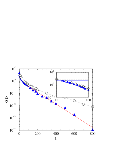
Figure 2: Average conductance $\langle G\rangle$ in units of $G_{0}$ versus length of the wire $L$ shown on a log scale. Tne number of scatterers is equal to the length, $N=L$ This keeps a well defined mean free path. Tne number of channels $M=5$. Triangles show results for the model, with an ensemble of $500$ scattering matrices $S$, each corresponding to a different configuration of randomly distributed over the wire $N$ point scatterrers. Note, that for long samples the mean conductance decreases exponentially with $L$, $\langle G\rangle\sim\exp(-L/\xi)$. The localization length, $\xi$, has been found by the least–square fit, to have a value $\xi=100\pm 3$ for $L>100$. Circles show results, when the scattering matrices have a block symmetry. The inset shows a double-log scale plot of the quasi-diffusive region, for $10<L<100$, for the $S$-matrices ensemble with and without block symmetry compared to the RMT predictions.

In the same figure there are shown also results for the ensemble of $S$-matrices with the block symmetry BS (open circles). The block symmetry is obtained, when the distributed point scatterers have a mirror symmetry with respect to the $y$-axis (that is $N/2$ points have been randomly distributed for $x\in(-L/2,0)$ and $y\in(0,\pi)$ and then the other $N/2$ have been obtained by the transformation $x\rightarrow-x,\quad y\rightarrow y$.

The inset in Figure (2) presents a double–log scale plot of the so called “quasi–diffusive” region, for $10<L<100$, for the $S$-matrices ensemble with and without block symmetry compared to the RMT predictions. Note, that there is an interval, where the mean conductance is roughly inversly proportional to $L$, $<G>\sim L^{-c}$. Fitted value $c=0.90\pm 0.05$ is close to 1.

In order to illustrate further the intermediate, quasi-diffusive regime, let us consider the variance of the conductance for discussed above ensembles of $S$–matrices. Figure (3) shows dependence of the variance of the conductance on the sample size $L$.

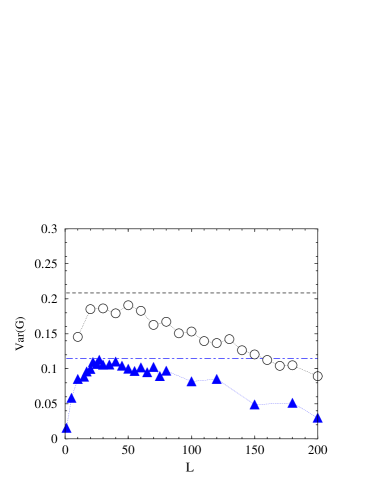
Figure 3: Variance of the conductance Var(G) as a function of the sample size $L$. The TRS is present. Number of channels $M=5$. Triangles show results without $S$-matrix block symmetry, and circles with that symmetry imposed. Horizontal lines depict the RMT predicitions for both BS, and no BS present.

Note that there is a narrow interval in sample lengths $L\in(20,50)$, where the variance weakly depends on the sample length. This defines the intermediate (quasi-diffusive) transport regime, which separates regimes of the ballistic and localized transport.

It is interesting to look into details of the $S$-matrix statistics in the intermediate regime, and see if it bears any deeper resemblance to the diffusive regime than just the fact, that the mean value of the conductance and its variance have close values to the ones predicted by the RMT. Let us inspect Figure (4).

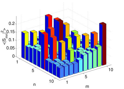
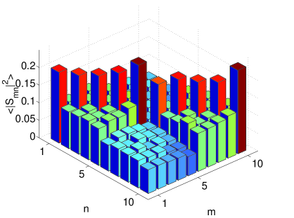
Figure 4: Averege over ensemble of squared absolute values of the $S$-matrix elements. The left panel shows raw data, whereas the right panel presents the data after unfolding procedure. Note, that after unfolding, it becomes clear that there exists enhancement on the diagonal. This indicates, that scattering back to the same channel is twice (roughly) larger than scattering back to a different channel.

Figure (4) presents averege of squared absolute values of $S$-matrix elements evaluated for an ensemble of 1000 $S$–matrices. In general however, an ensemble of $S$–matrices describing the scattering in the model wire for a number of configuration of $N$ impurities does not necessarily comply with the asumption for the RMT ensemble, saying that the average of the matrix elements over the ensemble vanishes. This requirement is usually met in the pure diffusive regime in the quantum chaotic scattering, where there is no direct processes present. The left panel of the figure shows raw data, whereas the right panel presents the data after unfolding procedure described in FM85 . This procedure transforms the “raw” ensemble into an equivalent ensemble, whose average over the ensemble vanishes $\langle S\rangle=0$. It is clear, that after removing “direct components” (i.e. a memory of the incdent channel), there is much better agreement with Equation (16), describing an enhancement on the diagonal. This indicates the fact, that scattering back to the incident channel is indeed roughly twice as large than scattering back to a different channel. Therefore in the present model we recover a well known universal result.

It is interesting to note, that the nearest neighbour NNS statistics, both for raw $S$-matrix eigenphases and unfolded data exhibit the Wigner behaviour — see Figure (5).

$$P(s)=\frac{s\pi}{2}\exp\left[-\frac{s^{2}\pi}{4}\right],$$ (21)

where $s$ denotes the spacing of the $S$-matrix eigenphases. This means that the NNS statistics, $P(s)$, is not so sensitive in revealing the universality regime, which complies fully with the RMT requirements and predicitons.

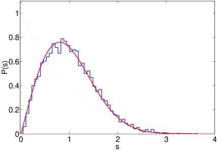
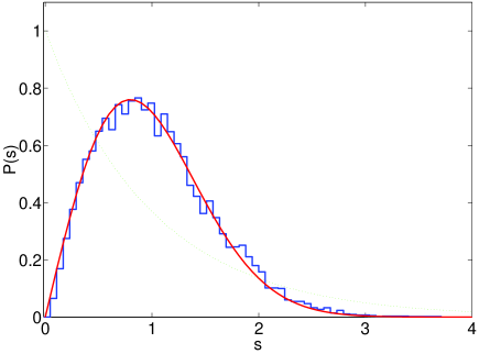
Figure 5: Nearest neigbour statistics, $P(s)$, for raw data (left panel) and unfolded data (right panel). Parameters the same as in Figure (4) . Note that there is virtually no difference between results shown on both panels. Both panels show a good agreement with the Wigner surmise (red curve). For a reference, there is also shown a Poisson distribution $P(s)=\exp(-s)$ (green curve).

In summary, the “quasi–diffusive” regime disscussed above bears some resemblance to the universal diffusive regime at the microscopic level, where the standard RMT theory of transport B97 holds, provided that one looks at statistical properties of the fluctuations around mean values of the $S$-matrix ensemble rather that considers the “raw” ensemble itself. At the macroscopic level, the conductance shows up some indication of the “ohmic behaviour”, that is $\langle G\rangle\sim 1/L$, and the variance of the conductance is weakly dependent on the sample size. The “quasi–diffusive” regime of transport is a transition regime between the ballistic transport and the

In Figure (2) we have seen that for $L>100$ one can see exponential decay of averaged over ensemble conductance. Instead of conductance itself let us look at logarithm of conductance. Figure (6) presents both average (filled dots) and variance (filled squares) of the logarithmic conductance. The inset shows the corelation between variance and the average of ${\rm ln}G$. The fitted slope $1.99\pm 0.05$ is in perfect agreement with the theoretical prediction of 2. This result supports a claim, that this regime is indeed characterized by the localization in electronic transport through the model quantum wire. Again considered model captures well features of the Anderson localization.

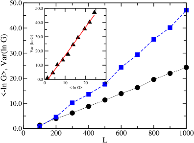
Figure 6: Average logarithmic conductance (filled dots) and variance of the logarithmic conductance (filled squares) as a function of the sample length. The inset ilustrates corelation between average and the variance of the logarithmic conductance ${\rm ln}G$. Each point corresponds to a different sample length $L$. The inset shows correlation between the variance and the average of the ${\rm ln}G$.

In order to see some more details of the transport mechanism, let us consider time delay distributions in the region of the localized transport. Figure (7) shows a distribution of logarithms of of the time delay, $\log\tau$ for $L=200$ and $L=800$. For longer samples ($L=800$), the distribution shows well pronounced maximum for time delays that are one order of magnitude longer than in the case of shorter samples ($L=200$).

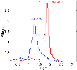
Figure 7: Distribution of logarithms of time delays, ${\rm log}\tau$ for $L=N=200$ and $N=L=800$.

Figure (8) presents the tail of the distribution $P(\tau)$ of time delays obtained for an ensemble of $10^{4}$ scattering matrices. The distribution resulting from adopted here theoretical model is compared with a theoretical prediction of TC99 . The fitted curve on the right panel of Figure (8) has been derived for a one-dimensional random potential in TC99 and reads:

$$P(\tau)=\frac{\xi}{2k\tau^{2}}\exp\left[-\frac{\xi}{2k\tau}\right]$$ (22)

The localization length $\xi$ is taken to have a value of 100 (as computed above) and $k=5.5708$. Thus presented here two-dimensional model essentially behaves like one-dimensional model in the limit of long times. Therefore also with this respect, the model exhibits a generic behaviour.

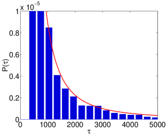
Figure 8: Time delay distribution $P(\tau)$ for $L=N=400$. Note a good agreement with the prediction for a one-dimensional random potential in the tail of the distribution (solid curve). There is $10^{4}$ $S$-matrices in the ensemble to calculate this distribution.

IV SUMMARY

Presented continuous and solvable (though not in a form of closed analytical expressions) model of electronic transport in disordered quantum wires is capable of reproducing a whole range of universal phenomena. Both micro ($S$-matrix statistics) and macro (conductance) signatures show consistant features of the ballistic, intermediate “quasi-diffusive” and Anderson localization regime in the transport. Results of the model agree very well with the predictions of the standard transport theory based on the RMT for a wide range of parameters. This allows to identify regimes of universal behaviour of the system. Moreover, thanks to flexibility and simplicity, presented model offers interesting possibilities of extending the standard transport approach beyond the quasi one–dimensional case in the regime of diffusive scattering.

References

- (1) C. W. J. Beenakker, Rev. Mod. Phys 69 731 (1997).
- (2) P. Exner, P. Gawlista, P. Šeba and M. Tater, Ann. Phys. 252 133 (1996).
- (3) R. A. Jalabert and J.-L. Pichard, J. Phys. I France 5 287 (1995).
- (4) R. Gȩbarowski, P. Šeba, K. Życzkowski and J. Zakrzewski, Eur. Phys. J. B 6 399 (1998).
- (5) C. Texier and A. Comtet, Phys. Rev. Lett. 82 4220 (1999).
- (6) K. Życzkowski, Phys. Rev. E 57, 2257 (1997).
- (7) N. Lehmann, D. V. Savin, V. V. Sokolov, and H.-J. Sommers, Physica D 86, 572 (1995).
- (8) W. A. Friedman and P. A. Mello, Ann. Phys. 161, 276 (1985).
- (9) R. Blümel, U. Smilansky, Phys. Rev. Lett. 60, 477 (1988).
- (10) H. U. Baranger, P. A. Mello, Phys. Rev. Lett. 73, 142 (1994).
- (11) E. Wigner, Phys. Rev. 98, 145 (1955).
- (12) F. T. Smith, Phys. Rev. 118, 349 (1960).