Subaru and Swift observations of V652 Herculis: resolving the photospheric pulsation

Abstract

High resolution spectroscopy with the Subaru High Dispersion Spectrograph, and Swift ultraviolet photometry are presented for the pulsating extreme helium star V652 Her. Swift provides the best relative ultraviolet photometry obtained to date, but shows no direct evidence for a shock at ultraviolet or X-ray wavelengths. Subaru has provided high spectral and high temporal resolution spectroscopy over 6 pulsation cycles (and eight radius minima). These data have enabled a line-by-line analysis of the entire pulsation cycle and provided a description of the pulsating photosphere as a function of optical depth. They show that the photosphere is compressed radially by a factor of at least two at minimum radius, that the phase of radius minimum is a function of optical depth and the pulse speed through the photosphere is between 141 and 239  $\mbox{km}\,\mbox{s}^{-1}$ (depending how measured) and at least ten times the local sound speed. The strong acceleration at minimum radius is demonstrated in individual line profiles; those formed deepest in the photosphere show a jump discontinuity of over 70 $\mbox{km}\,\mbox{s}^{-1}$ on a timescale of 150 s. The pulse speed and line profile jumps imply a shock is present at minimum radius. These empirical results provide input for hydrodynamical modelling of the pulsation and hydrodynamical plus radiative transfer modelling of the dynamical spectra.

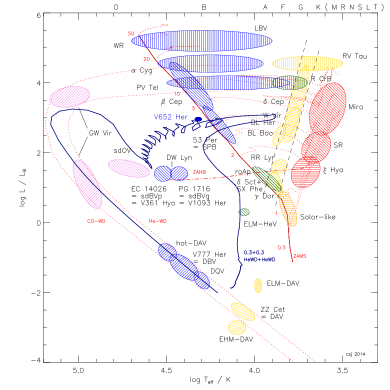
Figure 1: Luminosity-effective temperature (or Hertzsprung-Russell) diagram showing the position of V652 Her (Jeffery et al., 2001) and the post-merger evolution track for a double helium white dwarf binary (0.3+0.3  $\rm M_{\odot}$: thick blue line: Zhang & Jeffery 2012). The latter shows expansion to become a yellow giant following helium-shell ignition. As the helium-burning shell migrates towards the core, the star contracts through a series of loops caused by helium-shell flashes, until it reaches the helium main-sequence. On completion of core helium burning, the star returns to the white dwarf cooling track. Although V652 Her is located below the main-sequence in the HR diagram, it is spectroscopically a giant; historically, the latter is a spectroscopic term and depends on luminosity-to-mass ratio (or surface gravity). In the case of the 0.6  $\rm M_{\odot}$V652 Her, this is higher (lower) than for main-sequence stars of the same effective temperature. Also shown are the approximate locations of other pulsating variables coloured roughly by spectral type, the zero-age main sequence and horizontal branch, the Cepheid instability strip, and evolution tracks for model stars of various masses, indicated by small numbers ( $\rm M_{\odot}$). Shadings represent opacity-driven p-modes ($\backslash\backslash\backslash$), g-modes (///) and strange modes ($|||$) and acoustically-driven modes ($\equiv$). Approximate spectral types are indicated on the top axis. Based on figures by J. Christensen-Dalsgaard and subsequently by Jeffery (2008).

Table 1: Published surface, pulsation and other properties of V652 Her. Users should refer to original publications. Notes. 1:Kilkenny et al. (2005), 2:Jeffery et al. (2001), 3:Przybilla et al. (2005), 4:Jeffery et al. (1999).

$P_{0}$ (1974)	$0.107\,992\,82\pm 0.000\,000\,02$		d	1
$\dot{P}/P$	$-7.426\pm 0.005\times 10^{-8}$		d d-1	1
$\langle T_{\rm eff}\rangle$ (ion equil)	22 930	$\pm 10$	K	2
$\langle\log g\rangle$ (He i lines)	3.46	$\pm 0.05$	$\mbox{cm}\,\mbox{s}^{-2}$	2
$\langle T_{\rm eff}\rangle$ (total flux)	20 950	$\pm 70$	K	2
$\langle R\rangle$	2.31	$\pm 0.02$	$\rm R_{\odot}$	2
$\langle L\rangle$	919	$\pm 014$	$\rm L_{\odot}$	2
$M$	0.59	$\pm 0.18$	$\rm M_{\odot}$	2
$d$	1.70	$\pm 0.02$	kpc	2
$T_{\rm eff}$ (NLTE)	22 000	$\pm 500$	K	3
$\log g$ (NLTE)	3.20	$\pm 0.10$	$\mbox{cm}\,\mbox{s}^{-2}$	3
$n_{\rm H}$ (NLTE )	0.005	$\pm 0.0005$		3
$T_{\rm eff}$ (mean)	24 550	$\pm 500$	K	4
$\log g$ (mean)	3.68	$\pm 0.10$	$\mbox{cm}\,\mbox{s}^{-2}$	4
$\log n_{\rm H}$	–2.16	$\pm 0.07$		4
$\log n_{\rm He}$	0			4
$\log n_{\rm C}$	–4.40	$\pm 0.27$		4
$\log n_{\rm N}$	–2.61	$\pm 0.06$		4
$\log n_{\rm O}$	–4.00	$\pm 0.08$		4
$\log n_{\rm Fe}$	–4.14	$\pm 0.15$		4

1 Introduction

Just over fifty years ago, Berger & Greenstein (1963) used the Palomar 5-m (200-inch) telescope to show that the early B star BD$+13^{\circ}3224$ is hydrogen deficient and a probable subdwarf. Whilst all permitted neutral helium lines were visible, the hydrogen Balmer lines were unexpectedly weak, although still detectable. A decade later, Landolt (1975) discovered light variations with a period 0.108 d and an amplitude of 0.1 mag (in $V$) in a star lying outside any known pulsation instability strip. Spectroscopic confirmation that BD$+13^{\circ}3224$ (V652 Herculis; Kukarkin et al. 1977) is a radially pulsating variable caused as much interest as the shape of its radial velocity curve (Hill et al., 1981; Lynas-Gray et al., 1984; Jeffery & Hill, 1986). The latter shows a very rapid acceleration around minimum radius followed by a constant deceleration covering nine tenths of the pulsation cycle. The maximum surface acceleration reaches some $300{\rm\,m\,s^{-2}}$, or $30g$ in terrestrial terms, and poses several questions that this paper addresses. To set these in context, we first reprise our current knowledge of V652 Her.

Additional multiwavelength photometry and ultraviolet observations from the International Ultraviolet Explorer (IUE) enabled the radius and distance to be obtained (Hill et al., 1981; Lynas-Gray et al., 1984) using the Baade-Wesselink method (Baade, 1926; Wesselink, 1946). The best radius measurement to date is $2.31\pm 0.02~{}{\rm R_{\odot}}$ which, with a surface gravity measured from the spectrum, gives a mass of $0.59\pm 0.18\,{\rm M_{\odot}}$ (Jeffery et al., 2001). Analysis of the spectrum shows a surface that is mostly normal in metal abundances, except for carbon and oxygen, which are weak, and nitrogen, which is sufficiently overabundant to demonstrate that the surface helium is the product of nearly complete CNO burning (Jeffery et al., 1999). The 0.5 per cent contamination by hydrogen represents a potential puzzle (Przybilla et al., 2005).

An apparent error in the predicted time of minimum radius (Hill et al., 1981), prompted Kilkenny & Lynas-Gray (1982) to show that the pulsation period had been decreasing since its first measurement, with subsequent observations of the light curve demonstrating up to third-order behaviour in the ephemeris (Kilkenny & Lynas-Gray, 1984; Kilkenny, 1988; Kilkenny & Marang, 1991; Kilkenny et al., 2005). The linear term is consistent with a secular radial contraction of some 30 km yr^-1, assuming a standard period – mean density relation.

At the time of discovery, no known mechanism could excite the pulsations in V652 Her (Saio, 1986). Not even the strange modes which drive pulsations in more luminous B-type helium stars would work for V652 Her (Saio & Jeffery, 1988). However, the development of improved opacities for the Sun and other stars and the discovery of additional opacity from iron group elements at $\approx 2\times 10^{5}$K (Rogers & Iglesias, 1992; Seaton et al., 1994) provided an explanation; pulsation driving is provided through the classical $\kappa$-mechanism (Saio, 1993). Non-linear calculations subsequently reproduced the period, light and velocity curves with satisfactory precision (Fadeyev & Lynas-Gray, 1996; Montañés Rodríguez & Jeffery, 2002).

In seeking an evolutionary origin for V652 Her, single star models are unable to explain all of the observed properties, although Jeffery (1984) argued that a star contracting towards the helium main-sequence could match the mass, luminosity and contraction rate. Such configurations might arise as a result of a late or very-late helium-core flash in a star that has already left the giant branch (Brown et al., 2001). Such a star could share the observed properties of V652 Her (Table 1). For the surface to be extremely hydrogen-deficient, a binary companion would be necessary to remove most of the red-giant envelope either by common-envelope ejection or by stable mass transfer. In the case of V652 Her, there is no evidence for a stellar-mass companion (Kilkenny et al., 1996). It is possible that high-order terms in the pulsation ephemeris might be caused by light-travel delays across an orbit around a planetary-mass companion having a period $8-12$ y (Kilkenny et al., 1996; Kilkenny et al., 2005).

The most successful model for the origin of V652 Her is that of the merger of two helium white dwarfs (Saio & Jeffery, 2000); following such a merger, the ignition of helium in a shell at the surface of the accretor and at the base of the accreted material creates a yellow giant, which subsequently contracts at a rate and luminosity commensurate with observation (Fig. 1), ultimately to become a helium-rich hot subdwarf (Zhang & Jeffery, 2012).

There might, therefore, seem to be little left to learn from V652 Her (Table 1). However, in obtaining the highest precision measurement of the radial velocity curve to date, Jeffery et al. (2001) noted that the extreme acceleration at minimum radius could be associated with a shock travelling outwards through the photosphere. Jeffery et al. (2001) identified possible line splitting in strong lines around minimum radius as supporting evidence for the idea of a shock. Fadeyev & Lynas-Gray (1996) predicted that a shock at minimum radius should be associated with a spike in the light curve; none has been detected in visible light (Kilkenny et al., 2005) and the ultraviolet light curve is too sparsely sampled to show such a feature (Lynas-Gray et al., 1984; Jeffery et al., 2001). Since the absence of hydrogen renders the stellar photosphere much less opaque than is normally the case, sufficiently high precision observations would offer unique opportunities (a) to establish whether a shock does indeed occur and (b) to explore the effect of pulsation on the photosphere itself. Since previous applications of the Baade-Wesselink method have relied on model atmospheres in hydrostatic equilibrium, higher precision data would also provide the opportunity to implement high accuracy dynamical models of the envelope and photosphere.

Another question prompted by the almost uniform surface acceleration between radius minima is how close the surface motion is to a ballistic trajectory. A simple picture of V652 Her likens the pulsating surface to a rocket that is rapidly accelerated upwards, after which it is in free fall until it returns to its original state near minimum radius, at which point the cycle repeats. The physics of the atmosphere of such a “rocket star” is of considerable interest.

Scrutiny of the published parameters for V652 Her (Table 1) raises further questions. Application of the classical period–mean-density relation $P\sqrt{\bar{\rho}/\bar{\rho_{\odot}}}=Q$ (Shapley, 1914) using the Jeffery et al. (2001) mass and radius and with a pulsation constant $Q\approx 0.033$ d (Fadeyev & Lynas-Gray, 1996) indicates an unacceptably long period of 0.15 d and implies that the measured surface gravity is too low by a factor of 2. Appealing to other measurements of the surface gravity, Przybilla et al. (2005) found a substantially lower value (at maximum radius) even though their model techniques were more sophisticated, while analyses using older methods had found higher values (Jeffery et al., 1999). Reconciling the spectroscopic and pulsation parameters for V652 Her represents a challenge for both theory and observation.

In this paper we present a unique set of spectroscopic observations of V652 Her. We describe the spectrum and present the radial velocity and equivalent width measurements obtained for each line. Using these data we explore the radial velocity behaviour of the photosphere in terms of its vertical structure. We explore the behaviour of line profiles throughout the pulsation cycle, and especially around minimum radius, including both strong and weak lines. We also present observations aimed at detecting evidence for a shock at ultraviolet and X-ray wavelengths. The result is a unique empirical description of the behaviour of the outer layers of a pulsating star, resolved over nearly three decades of optical depth.

Figure 2: Swift UVOT photometry of V652 Her from 2010 May 6, phase folded using the ephemeris given in § 4.2. The systematic uncertainty is marked separately.

Figure 3: IUE photometry of V652 Her re-extracted at $\lambda_{\rm c}=2246$ Å, $\Delta\lambda=498$ Å, and phase folded using the ephemeris given in § 4.2.

Figure 4: NGTS visual photometry of V652 Her from 2010 May 6, phased using the ephemeris given in § 4.2.

2 Observations: Swift and NGTS photometry

Observations were made with all instruments on board the gamma-ray burst detecting satellite Swift (Gehrels et al., 2004) on 2010 May 6 during a target of opportunity programme (obsID 00031714). Six observations, with a total exposure of $\sim$7 ks, were carried out at intervals intended to cover different phases of the light curve. V652 Her was not detected at high energies, as expected, with a 3$\sigma$ upper limit on the 0.3-10 keV X-ray count rate of $1.25\times 10^{-3}$ count s^-1 (using the Bayesian method) for all six observations combined. It was only detected with the UV/Optical telescope (UVOT) observing in the UVM2 filter ($\lambda_{\rm c}=2246$ Å). V652 Her is close to the bright limit for the UVOT and therefore a special calibration was required to extract reliable photometry (Page et al., 2013). This calibration has been applied; the resulting photometry in Vega magnitudes and phased to the most recent ephemeris (§ 4.2) is shown in Fig. 2. A systematic uncertainty of $\pm 0.1$ mag should be added to these measurements, as deemed necessary by Page et al. (2013), who suggest that the method be limited to stars fainter than ninth magnitude, while V652 Her is brighter than this by a few tenths or so. However, the photometry is considered accurate to within the $1\sigma$ errors shown.

There is a discrepancy between the Swift UVOT photometry obtained in 2010 and the IUE photometry obtained between 1979 and 1984 as reported by Lynas-Gray et al. (1984) and Jeffery et al. (2001). The photometry has been re-extracted to form equivalent Vega magnitudes in a bandpass centred around 2246 Å having the same FWHM (full width at half maximum) as the UVM2 filter (498 Å); the results are shown in Fig. 3. It will appear from these data that, modulo the systematic error in the UVOT zero point, V652 Her may have brightened at 2246 Å by $\approx$0.5 mag in the 30 yr since first observed at these wavelengths.

Recall from § 1 that the observed change in pulsation period is consistent with a secular radial contraction of some $30{\rm\,km\,yr^{-1}}$ for a star with a radius of 2.3 $\rm R_{\odot}$ and a mean effective temperature (in 2000) around 23 000 K. Assuming a constant luminosity (for the sake of argument, but consistent with evolution models), such a contraction would correspond to an increase in effective temperature of some $100{\rm\,K\,yr^{-1}}$. Considering the 30 yr elapsed between the IUE and UVOT observations, the effective temperature of V652 Her should have increased by some 3000 K. Under the constant luminosity assumption, this implies a dimming by $\approx$0.15 mag at 2246 Å, and brightening at shorter wavelengths. It is therefore not, at present, clear where the UVOT/IUE discrepancy arises.

Broad-band optical photometry was obtained on the same day as the Swift observations, with the Next Generation Transit Survey (NGTS) prototype on La Palma (McCormac & et al., 2014), a 20 cm Takahashi telescope with a 1k$\times$1k e2v CCD operating in the bandpass $600-900$ nm. The NGTS-P data were bias subtracted and flat-field corrected using PyRAF and the standard routines in IRAF and aperture photometry was performed using DAOPHOT (Stetson, 1987). Only relative fluxes were obtained, since the bandpass is custom made and standard stars were not observed. Due to weather conditions, only the part of the light curve leading to and including visual light maximum was observed. Phased to the same ephemeris, these data are shown in Fig. 4 and, as far as is possible for these data, confirm the ephemeris is correct for the date of the Swift observations.

3 Observations: Subaru spectroscopy

Observations were obtained with the High Dispersion Spectrograph (HDS) (Noguchi et al., 2002) of the Subaru telescope on the nights of 2011 June 6 and 7 (Julian dates 2455719–20). A total of 772 spectra were obtained in pairs to cover the wavelength ranges $398.7-482.2$ nm and $487.3-570.6$ nm (386 spectra in each range), all with an exposure time of 120 s and spectral resolution of $R=90\,000$. The mean time between exposures for read out of the detectors was $\approx$56 s. The median signal-to-noise (S/N) ratio in the continuum region around $452-453$ nm was 73 on the first night and 58 on the second night. At the epoch of these observations, the exposure time corresponds to 0.013 pulsation cycles, whilst the mean sampling interval corresponds to $\approx$0.020 cycles, which had slightly unfortunate consequences for the phase distribution.

Thorium-argon (ThAr) comparison lamp exposures were obtained at the beginning and middle of each night. For wavelength calibration, the ThAr spectrum obtained in the middle of each night was used. The CCD images were processed using IRAF and ESO-MIDAS software to extract and merge the échelle orders to obtain one-dimensional (1D) spectra.

The overscan data were processed using IRAF and a cl script from the Subaru website (http://subarutelescope.org/Observing/Instruments/HDS/index.html). This script also subtracted the average bias from each frame. To extract and merge the échelle orders to 1D, the fits files were converted to ESO-MIDAS internal format. Each 2D frame was rotated so that the échelle orders were approximately horizontal with wavelength increasing along each order from left to right and order number increasing from top to bottom (as viewed on screen). For each observing night an average image was constructed using 50 object frames obtained in the middle of the night. These average images were used to determine the order positions. Order detection was done using a Hough transform (Ballester, 1994). The ESO-MIDAS command for order definition also provides an estimate of the background in the interorder space. Échelle orders were extracted by taking a sum of pixel values over the slit with one pixel width running along the orders. The length of the slit was defined using the average object frame.

Each extracted order was normalized to a smooth continuum. This smooth continuum was obtained using a polynomial approximation to the median-filtered extracted orders, avoiding spectral lines. When an order has strong lines with broad wings, the continuum for that order was calculated by interpolation between neighbouring orders.

For wavelength calibration, ThAr spectra were extracted from 2D images. Spectral lines were detected in the extracted orders and line centres were determined by Gaussian fitting. Several lines were identified on the 2D images and global dispersion coefficients were derived by comparing these lines with the ThAr line list. Dispersion coefficients for each order were calculated from the global coefficients and used to make a polynomial approximation to the wavelength scale for each order.

The extracted orders were resampled at constant wavelength intervals and merged into a 1D spectrum for further analysis.

Figure 5: The median formal error in the CoG radial velocity errors $\langle\sigma_{v}\rangle$ as a function of the median equivalent width $\langle W_{\lambda}\rangle$ for each line.

4 Velocity Measurement

4.1 Line measurements

We first identified a number of lines covering a broad range of atomic species, multiple ions for the same species and a wide range of excitation potentials and oscillator strengths for given ions. For each of these we required a radial velocity, equivalent width and associated errors.

For each line, we identified a segment of spectrum (wavelength interval) that covers the single line in all phases. This segment was extracted from each spectrum and a smoothed version of each segment was formed using a median filter. The smoothed spectrum was used to estimate the maximum depth in the line and hence to make a preliminary estimate of the line centre. The centre of gravity (CoG) of the line profile was obtained from the non-smoothed line segments, using a smaller segment of the profile with a fixed width centred on the preliminary line centre. The adopted widths are different for different lines and were estimated iteratively and interactively to obtain a measurement of the whole profile at all phases. This approach was used to obtain the line wavelengths and also the equivalent widths. The barycentric radial velocity for each line in each spectrum was obtained by comparing the CoG wavelength with the laboratory wavelength for that line and correcting for the Earth’s motion.

The measurements of weak lines are less reliable, especially when lines are broadened by a large expansion speed or effective surface gravity around minimum radius, where some lines become quite asymmetric or simply too weak to measure. Problems may also arise when there are strong nearby lines or blends and the measurement algorithm selects the wrong component. Such problems can be mitigated by using a smaller wavelength window, but this has the disadvantage of not including the whole line profile.

From the original line list covering 13 atomic species and 17 different ions identified in the spectrum of V652 Her, we obtained 50 952 radial velocity measurements covering a total of 132 lines from each of 386 Subaru spectra. Equivalent widths were measured from all 386 Subaru spectra for 125 lines, the smaller number being due to the dilution of some lines around minimum radius, and to blending.

The errors in the radial velocity measurements were obtained from the CoG measurement assuming a mean variance in each datum entering the calculation. For the most part, the mean formal error for each line was inversely correlated with the strength of the line (Fig. 5):

$$\log\langle\sigma_{v}\rangle\approx-2-(\log\langle W_{\lambda}\rangle+0.7).$$

In all cases, the mean errors were $\langle\sigma_{v}\rangle<0.2\,\mbox{$\mbox{km}\,\mbox{s}^{-1}$}$ for each line and overall $\langle\sigma_{v}\rangle=0.06\,\mbox{$\mbox{km}\,\mbox{s}^{-1}$}$.

The radial velocity and equivalent measurements are available in a single table as an on-line supplement described in Appendix A.

4.2 Ephemeris

To make further progress with verification and analysis of the line measurements, it was necessary to convert the times to pulsation phase. The times of mid-exposure were obtained from the image headers and supplied as geocentric modified Julian date. These were converted to barycentric Julian dates (BJD) using the FK5 (J2000) coordinates for V652 Her. We adopted the following ephemeris for times of maximum based on all times of maxima up to and including 2013 March (Kilkenny 2013, private communication):

$$T_{\rm max}=T_{0}+nP_{0}+n^{2}k_{1}+n^{3}k_{2}+n^{4}k_{3}$$

where $n$ is the cycle number and

$$\begin{split}T_{0}&={\rm BJD}2442216.80481,\\ P_{0}&=0.107992526~{}{\rm d},\\ k_{1}&=-44.533\times 10^{-10}\,{\rm d},\\ k_{2}&=+3.203\times 10^{-15}\,{\rm d},\\ k_{3}&=-3.919\times 10^{-21}\,{\rm d}.\end{split}$$

We note that the period in 2011 had decreased to 0.106994 d compared with 0.107995 d originally measured in 1974 by Landolt (1975).

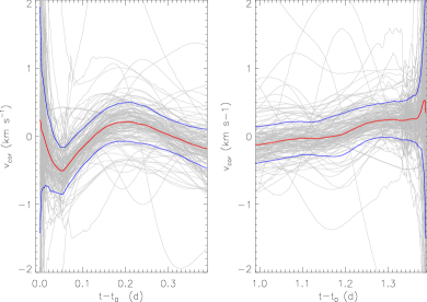
Figure 6: The time dependent component of the systematic velocity correction applied to all radial velocity measurements (solid red line). This correction is evaluated as the smoothed median of the individual line velocity differences (grey curves) measured relative to a “representative” velocity curve. The blue curves show the median curve $\pm$1 standard deviation. The nights of June 6 and 7 are plotted separately in the left- and right-hand panels. The most likely causes for these systematic shifts are temperature changes in the spectrograph and guiding errors on the fibre bundle.

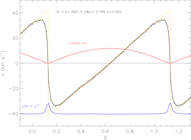
Figure 7: Absorption line velocities and related quantities as a function of pulsation phase for a single absorption line: in this case Nii 4621 Å. The line is identified by ion and wavelength, $\lambda$ (in Å). In addition, the mean equivalent width of the line, $W_{\lambda}$ (in Å), and the optical depth of formation of the line core, $\tau_{\rm c}$, are shown. The thin solid grey curve represents the reference velocity curve obtained from the median of 29 Nii lines. The thin straight orange lines are simply guides and represent infinite acceleration followed by uniform deceleration. Each ’+’ represents an individual radial velocity measurement, each colour refers to a single pulsation cycle, the measurement errors are smaller than the symbols. Radial velocity: the solid black curve represents the phase-averaged velocity curve, $v$, obtained from the line velocities ( $\mbox{km}\,\mbox{s}^{-1}$). Not shown: the de-projected surface expansion velocity $\dot{r}$ is obtained by correcting each line velocity by the appropriate factor (see text). Acceleration: the solid blue curve represents the first derivative of the phase averaged expansion velocity curve, $\ddot{r}$, offset by $-40$ and scaled $\times 20$. Thus, an acceleration reaching $-30$ on the $y$-axis corresponds to an acceleration of 200 m s^-2. Displacement: the solid red line represents the integral of the phase-averaged expansion velocity curve, $\delta r$, with a constant chosen such that the total displacement over one pulsation cycle is zero and, in this case, that minimum radius corresponds to a displacement of zero. A displacement of $+10$ on the $y$-axis corresponds to a radial displacement of 100 000 km.

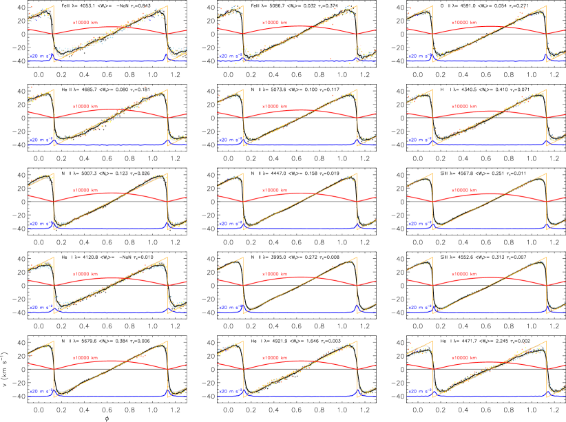
Figure 8: As Fig. 7 for an ensemble of absorption lines representing a range of species and strengths as labelled in each panel. A mean equivalent width $\langle W_{\lambda}\rangle={\rm-NaN}$ implies that a valid measurement was not obtained for that line. The phase shift of maximum acceleration with line depth is best seen by expanding this plot using a machine-readable version of this paper and a suitable reader.

4.3 Systematic errors

Comparing the radial velocity measurements from one line to another, and both radial velocity and equivalent width measurements from one pulsation cycle to the next, it was clear that two kinds of systematic error were present: constant and time dependent.

i) Plotting different lines as a function of phase, it was evident that the rest wavelengths used in each case were not consistent with one another. Since rest wavelengths were not always well specified, and in many cases lines are blended, these inconsistencies were intelligible and easily neutralized by the expedient of requiring the mean velocity averaged over all 386 measurements to be zero.

ii) Plotting velocities and equivalent widths as a function of time showed significant systematic shifts from one pulsation cycle to another leading to, for example, an apparent overall shift in the systemic velocity of up to $2\,\mbox{$\mbox{km}\,\mbox{s}^{-1}$}$ over two nights and a change in the average absorption line strength by a few per cent. Possible causes for the velocity shifts include motions due to an unseen companion and/or shifts in the wavelength calibration due to thermal fluctuations in the spectrograph and/or errors in guiding the star on the slit or fibre bundle. Causes for the equivalent width shift include inconsistency in continuum placement and/or background (sky, scattered light) subtraction. We have reduced, but not completely removed these systematic effects as follows.

To understand the slowly varying velocity shifts we first formed a mean radial velocity curve from a single strong line (Nii 3995 Å) averaged in phase over all cycles. We subtracted this mean curve from the observed velocity curve in the time domain, and examined the residual. During the first part of the first night, the residual velocity dropped evenly by 0.5 $\mbox{km}\,\mbox{s}^{-1}$ over 1 or 2 h, recovered sharply and remained approximately constant for the remainder of the night. On the second night, the residual increased by about 1.5 $\mbox{km}\,\mbox{s}^{-1}$ during the course of the night. We computed the same residual for all other lines. Apart from the weakest and noisiest lines, all lines showed similar behaviour.

Therefore, we established a phase-averaged velocity curve for each absorption line, subtracted this from the time domain velocity curve for each line, and smoothed the result over 1.2 (FWHM) pulsation cycles to give a slowly varying velocity correction for each set of radial velocity measurements (Fig. 6: grey curves). We computed a median and standard deviation from these corrections, smoothed the result over 0.12 (FWHM) cycles in the time domain and used this correction for all lines (Fig. 6: red and blue curves). The maximum amplitude of this correction was $<\pm 0.5\,\mbox{$\mbox{km}\,\mbox{s}^{-1}$}$. We investigated the mean residual between these corrected velocities and a phase-averaged radial velocity curve for each line, and found the mean cycle-to-cycle variation to lie below $\pm 0.4\,\mbox{$\mbox{km}\,\mbox{s}^{-1}$}$. Increasing the FWHM of the second smoothing function above had a relatively small effect on the overall results.

Similarly, for the slowly varying equivalent widths we formed a mean equivalent width curve for each line over a single cycle, and then formed the ratio of this curve with respect to the time varying curve, smoothed the ratio over 0.5 cycles and applied this slowly varying correction to the original equivalent width measurements.

4.4 Radial velocities

After correction for systematic shifts, all of the radial velocities were plotted as function of pulsation phase on figures similar to Fig. 7, a representative plot showing the data for the relatively strong Nii 4621 Å line. The velocities are shown as ‘+’ symbols and colour coded by pulsation cycle.

The first goal was to determine whether there are line-to-line differences in the radial velocity curves. In order to assess this, we formed a reference radial velocity curve from the average radial velocities of 29 strong Nii lines for which the lines were strong and present in all observations. These were ordered by phase and smoothed using a Gaussian filter with FWHM of 0.016 cycles. The radial velocities for each line measured were also ordered by phase, and smoothed using the same filter function. The reason for smoothing the data was to obtain as optimal a phase resolution as possible, using observations from successive pulsation cycles obtained at different phases to fill in the phase space. Limitations are provided by incomplete removal of the systematic cycle-to-cycle zero-point shifts, and a relatively non-uniform phase distribution of the data, despite observing nearly six distinct cycles without a formal constraint on the exposure start times. An experiment with a smaller Gaussian (0.012 cycles) resulted in increased errors resulting from the non-uniform phase distribution

We examined the difference in the sense of observed-minus-reference velocity for each line. In the case that an absorption line enters the rapid acceleration phase earlier than the reference line, the residual will show a trough centred at or before the point of maximum acceleration. If the absorption line accelerates later than the reference line, the residual will show a peak after maximum acceleration. Examples of both types of behaviour were readily identified.

The hypothesis is that deeper layers of the photosphere commence acceleration before higher layers as the “shock” propagates upwards through the photosphere. The assumption was that higher ionization species (e.g. Feiii, Siiv) would be formed deeper than lower ionization species (e.g. Siii, Nii). In fact, there were no systematic differences among Siii, iii and iv. What became clear was a strong systematic correlation between line strength (expressed as equivalent width) and acceleration phase.

This can be understood as follows. The central depth of an absorption line is a direct measurement of the position in the photosphere at which the line optical depth $\tau_{\lambda}$ is unity. In continuum regions, photons arrive from regions where the continuum optical depth $\tau_{\rm c}<1$. In line centres, photons arrive from layers where $\tau_{\lambda}<1$. If the atmosphere structure and composition are known, the relation between geometric depth and line optical depth can be computed. Alternatively, one can write the position at which $\tau_{\lambda}=1$ in terms of some continuum optical depth $\tau_{\rm c}$. For now, one only needs to recall that the deeper an absorption line, the higher in the photosphere that the core is formed, the limit being the layer above which scattering dominates over absorption.

This result is partially illustrated in Fig. 8, which presents the same information as Fig. 7 for 15 representative lines from the very weak Feiii 4053 Å to the very strong Hei 4471 Å.

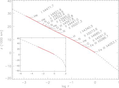
Figure 9: Detail from the run of geometric height above the continuum forming layer $z(\tau)-z(1)$ as a function of optical depth $\tau_{4000}$ in a model for the atmosphere of V652 Her (broken line). The line-forming region is marked as a solid red line. The locations of formation of the cores of the representative lines in Fig. 8 are indicated. The same function for the entire model atmosphere is inset.

5 Pulsation

To study the behaviour of each line individually and the photosphere represented by the entire ensemble, we have analysed the data as follows.

5.1 Model atmosphere

To establish where in the photosphere the core of each line is formed, we computed a representative model for the atmosphere of V652 Her (Behara & Jeffery, 2006) and its emergent spectrum (Jeffery et al., 2001). This model was selected using a median Subaru spectrum obtained between phases 0.60 and 0.70, and without any velocity corrections. This spectrum, and the adopted model are shown in Appendix B.

5.2 Photospheric structure

The model spectrum includes, for every line, the value of $\tau_{4000}$, the optical depth in the continuum at which the line optical depth is unity. The model also permits us to compute a relationship between $\tau_{4000}$ and the geometric depth relative to some reference point. In this case we adopt the layer where the continuum optical depth at 4000 Å is unity (Fig. 9). Thus the geometric position of the line core is established, assuming an equilibrium structure. For the present, we posit that, to first order, the structure of the photosphere at maximum radius matches this structure satisfactorily. For reference, Fig. 9 identifies the positions at which the cores of the representative lines shown in Fig. 8 are formed, showing that they cover nearly three decades in optical depth, and some 25 000 km in geometric depth (at maximum radius). To place some of these numbers in context, we note that the mean radius of $2.31\pm 0.02\mbox{\,$\rm R_{\odot}$}$ (Jeffery et al., 2001) corresponds to $\approx 1\,600\,000$ km. Consequently, the region of the star sampled by the absorption line cores represents $\approx 2\%$ of the radius.

5.3 Projection effect

The radial velocity $v$ measured for a spherically expanding star is diluted by projection effects (sometimes referred to as limb darkening), and so must be increased by a suitably chosen projection factor $p$ in order to represent the true expansion velocity of the star $\dot{r}$ (Parsons, 1972). Montañés Rodriguez & Jeffery (2001) studied this question for the general case of early type stars, for V652 Her in particular, and as a function of line strength. Following Parsons, they adopted a relation for the projection factor of the form

$$\dot{r}=-pv,$$

$$p=a_{0}+a_{1}\gamma$$

where

$$\gamma=-\dot{r}/w_{1/2}$$

and

$$w_{1/2}=\frac{\Delta\lambda_{1/2}c}{\lambda}$$

is the half width (in velocity units) at half depth of the line at wavelength $\lambda$. For the case of V652 Her, we adopt values from Montañés Rodriguez & Jeffery (2001) (Table 4, Case (b)):

$$a_{0}=1.402,a_{1}=-0.028.$$

Values for $\Delta\lambda_{1/2}$ were obtained from the same model spectrum used to establish the geometric structure of the photosphere. For $\gamma$, we adopt the first order approximation $\dot{r}=-1.38v$.

5.4 Displacement and acceleration

Having established $\dot{r}$ for each absorption line, it is straightforward to evaluate the local acceleration $\ddot{r}$ and displacement $\delta r$ by differentiating and integrating, respectively. The latter requires a boundary condition; we here require the displacement to be zero at maximum radius. These quantities are illustrated for selected lines in Figs. 7 and 8.

The choice of boundary condition allows us to add the geometric depth at which the line forms at maximum radius, as deduced above, and hence obtain, as a function of phase, the radial displacement from every line measured relative to a defined position, being where $\tau_{4000}=1$ at maximum radius. We also adjusted the zero-point of the velocity curve (a second time) to ensure that the total displacement over the pulsation cycle was zero.

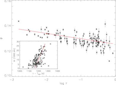
Figure 10: The phases of maximum acceleration obtained from 137 absorption lines as a function of optical depth of formation of the line cores. The linear fit to these data (red line) and $1\sigma$ errors are also shown. The inset panel shows the same information plotted as a function of geometric depth against time since $T_{\rm max}$.

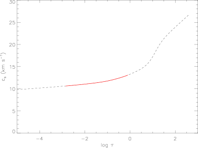
Figure 11: The local sound speed $c_{\rm s}$ in a hydrostatic LTE model atmosphere for V652 Her at maximum radius as a function of continuum optical depth (broken line). The line-forming region (Fig. 9) is shown as a solid red line.

5.5 Phase of minimum radius

The phase of minimum radius for each line was measured from the phase of maximum acceleration $\phi_{\ddot{r}_{\rm max}}$. We located the maximum by fitting a parabola to the acceleration curve, including up to 20 points within $\pm 0.05$ cycles of the largest value of $\ddot{r}$. The results are shown in Fig. 10 as a function of the line core optical depths. Although there is substantial scatter at large optical depths, where the absorption lines are weakest and hardest to measure, a trend is apparent. A linear fit giving the correlation,

$$\phi_{\ddot{r}_{\rm max}}=0.1254(2)-0.0042(1)\log\tau$$

is also shown in Fig. 10 (errors on final digits in parenthesis). This demonstrates that maximum acceleration, and hence minimum radius, occurs earlier in deeper layers, and supports the hypothesis stated in §4.4. The outward moving pressure wave emanating from the stellar interior that characterises the pulsation subsequently propagates upwards through the photosphere. Since we have a good estimate of the geometric depth in terms of optical depth (Fig. 9), the above correlation converts to a mean pulse speed through the photosphere $v_{\rm pulse}=239\pm 6\,\mbox{$\mbox{km}\,\mbox{s}^{-1}$}$ (Fig. 10 inset). For reference, the local sound speed in a stationary atmosphere for the model adopted to represent the star at maximum radius is shown in Fig. 11.

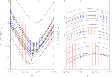
Figure 12: Top: the total radial displacement of different layers of the photosphere of V652 Her as represented by different groups of absorption lines. The lines are grouped by depth of formation at maximum radius into bins with $\delta\log\tau_{\rm c}=0.2$ centred at $\log\tau_{\rm c}=-0.1(0.02)-2.9$, and normalized using the $\tau-z$ relation shown in Fig. 9 such that a line formed at $\tau_{c}=0$ would have zero displacement at maximum radius. Consequently the weakest lines correspond to the lowest layers of the photosphere and vice versa. Bottom: Expansions of the upper panel around minimum and maximum radius. Since each curve represents the average of several lines within a bin, standard deviations (red) and standard errors in the mean (blue) have been added for three representative bins. The green diamonds represent radius minima for each line group obtained by fitting a parabola through the five points around minimum radius; the solid green line represents a regression on these minima (excluding Hei 4471Å) with a slope ${\rm d}\delta r/{\rm d}\phi\times{\rm d}\phi/{\rm d}t=141\pm 17\,\mbox{$\mbox{km}\,\mbox{s}^{-1}$}$.

5.6 Resolving vertical motion

Another way of representing the pulsation of the photosphere is by considering the radial displacement. The individual line displacements obtained by integrating $\dot{r}$ and adding the geometric depth of formation can be plotted as a function of phase. Owing to noise in the weaker lines, a plot showing all individual lines is not informative. By grouping lines in terms of $\tau_{c}$ and plotting the median displacement for each group, the time varying structure of the photosphere becomes apparent. We used uniform bin sizes $\delta\log\tau_{c}=0.2$ centred at $\log\tau_{c}=-0.1,-0.3,\ldots,-2.9$. Fig. 12 demonstrates how the photosphere is compressed by almost a factor of two as the star approaches minimum radius, and then recovers as the star expands. Again placing numbers in context, the mean pulsation amplitude of $\approx 120\,000$ km represents $\approx 8\%$ of the mean stellar radius. The top layer is represented by a single very strong line, Hei 4471 Å, for which radial velocities are difficult to measure. The bottom layers are represented by extremely weak lines which virtually disappear at minimum radius. However, the overall result holds well at all depths, and also reflects the phase dependence of minimum radius obtained using $\ddot{r}$ above. By fitting parabolae to each line group, an alternative estimate of the phase of radius minimum is obtained (Fig. 12: lower left). A regression on these locations gives the vertical velocity of minimum radius as $141\pm 17\,\mbox{$\mbox{km}\,\mbox{s}^{-1}$}$. Whilst this number is nearly a factor of 2 smaller than that obtained from the phases of maximum acceleration, the manner in which the displacements were obtained is significantly different.

It should be emphasized that the motion depicted in Fig. 12 is not Lagrangian. The displacements traced here refer to the locations of formation of the cores of specific groups of absorption lines. These locations move both with the bulk motion of the photosphere and within the photosphere as it is compressed and heated. In order to understand Fig. 12 in terms of the motion of mass, a theoretical model of the spectrum derived from an appropriate hydrodynamical model of the pulsating star will be necessary.

Whether the phase of maximum acceleration or of minimum radius is used, one thing is clear: the passage of either quantity through the photosphere is of the order of 10 times the value of the local sound speed.

5.7 He i 4471 Å

He i 4471 Å is difficult to measure for two major reasons. First, it is very strong, so the CoG method for velocity measurement requires a very broad window if it is to be consistent with other lines. However, this means that other lines become included in the blend. Second, the triplet and forbidden components, which form at different depths, are strongly blended and hence the line is asymmetric; moreover, due to the quadratic Stark effect and electron impacts, both the widths and rest wavelengths of the lines shift with density (Barnard et al., 1969). Consequently, in the context of pulsation, the line does not have a fixed rest wavelength, as was assumed for the velocity measurement. To some extent, other diffuse lines including He i 4921 Å and 4026 Å suffer from the same problem.

5.8 Surface trajectory

In § 1, V652 Her was introduced as ‘the rocket star’ because of its characteristic pulse-coast-pulse shaped radial velocity curve. Since the ‘coasting’ phase appears almost linear, one might ask how closely the surface motion follows a ballistic trajectory. Applying the projection factor described above, the mean acceleration $\langle\ddot{r}\rangle=-12.1\pm 0.4~{}{\rm m\,s^{-2}}$ between $0.3<\phi<1.0$ over all N ii lines. It is not exactly linear (Figs. 7, 8), but increases in amplitude from $-10.9$ to $-12.5{\rm m\,s^{-2}}$ between the first and the second halves of this interval.

For comparison, the gravitational acceleration of a star with $R=2.3\mbox{\,$\rm R_{\odot}$}$, and $M=0.59\mbox{\,$\rm M_{\odot}$}$ is twice this value with $g=-25~{}{\rm m\,s^{-2}}$ (corresponding to $\log g=3.4$ in cgs units). Since the radial displacement (120 000 km) is not small compared with the radius, the true surface gravity varies between $-26~{}{\rm m\,s^{-2}}$ at minimum radius, and $-23~{}{\rm m\,s^{-2}}$ at maximum. A ballistic trajectory would be symmetric around maximum displacement.

Thus the observed surface trajectory is not truly ballistic, and the increasing deceleration is presumably due to a more gradual decay in internal pressure following the major pulse at minimum radius. If the surface trajectory were to be closer to ballistic, the effective gravity acting on the photosphere would be much reduced, with significant consequences for the spectrum.

6 Line Profile Variations

The principal advantages of using one radial velocity measurement per absorption line per spectrum are the limitation in the number of data and the relative simplicity of interpretation. A disadvantage of the CoG approach is that additional information provided by the whole line profile is lost. At large radii, the near ballistic atmosphere should show narrow absorption lines characteristic of low surface gravity whilst, around minimum radius, the accelerating atmosphere should show broader lines characteristic of high surface gravity. In between times, the lines are intrinsically asymmetric due to projection effects from the spherical surface. In addition, around minimum radius and where conditions permit, there is the possibility of observing both inward-falling and outward-rising material in the same absorption line. This would be indicative of highly compressed and possibly shocked material. This section seeks to interpret the line profile variations over the pulsation cycle of V652 Her.

Figure 13: The phase folded spectrum of V652 Her around the Hei 4471 Å and Mgii 4482 Å lines and around minimum radius. The top panel shows the individual normalized spectra ($A_{\lambda}$), offset vertically upwards by an amount proportional to phase $\phi$. The middle panel shows the same data after application of a 4-pixel median filter in the dispersion direction. The bottom panel shows the data after application of a Gaussian filter in the phase direction with FWHM = 0.024 cycles.

6.1 Optimizing signal-to-noise ratio

Although the S/N ratio of most individual spectra is high, the number of spectra obtained close to minimum radius is relatively small, the exposure time relative to the acceleration phase is significant, and the effects of gravity broadening and acceleration smearing dilute information at these phases. However, there are two major ways in which the S/N ratio can be further increased. First, the resolution of the Subaru data (90 000) is sufficiently high that the intrinsic profiles of even the weakest lines are oversampled. Secondly, by effectively observing eight passages through minimum radius over the two nights we can increase the S/N by folding the data in phase. One approach would be to bin the data in both wavelength and phase; we have rejected this to avoid losing information unwittingly. Instead, we have applied a 4-pixel median filter in the dispersion direction and then applied a Gaussian filter with an FWHM of 0.012 cycles in the phase direction. The result is demonstrated for the Hei 4471 Å and Mgii 4482 Å lines around minimum radius in Fig. 13. Since the Gaussian filter has an FWHM comparable with the duration of a single exposure (0.013 cycles), little information is lost.

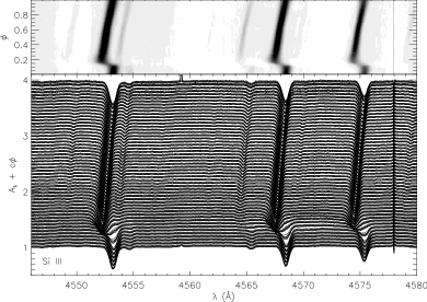
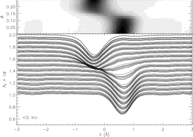
Figure 14: The behaviour of the strong Siiii triplet over a complete pulsation cycle (top) and around minimum radius (bottom). In each pane, the lower panel represents the continuum normalized flux as a function of wavelength, with a constant added which is proportional to the phase. The upper panel represents a grey-scale plot containing the same information. Features which do not change in wavelength as a function of phase are instrumental artefacts. The bottom panel represents the mean of all three Siiii lines. The wavelength scale is relative to the rest wavelength for each line. The data have been phase smoothed (see Fig. 13).

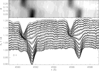
Figure 15: The behaviour of two intermediate strength Oii lines around minimum radius. The data have been phase smoothed (see Fig. 13).

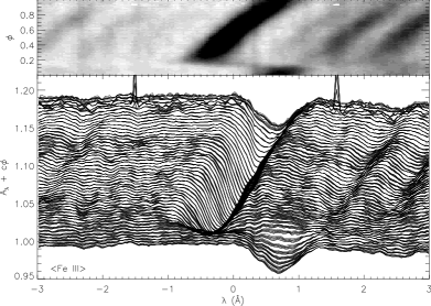
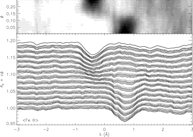
Figure 16: The behaviour of six weak Feiii lines represented as a composite line profile relative to the line rest wavelength. The wavelength scale is relative to the rest wavelength for each line. The data have been phase smoothed (see Fig. 13).

6.2 Line behaviour

Figs 14 - 16 illustrate the behaviour of a number of individual absorption lines over the whole pulsation cycle and expanded over the phase around minimum radius. In the cases of strong lines, this behaviour is relatively easy to identify. The two obvious features are (a) narrowing of the lines from phases 0.3 to 0.65, followed by broadening, and (b) the sharpness of the transition from contraction to expansion. Qualitatively speaking, the transition appears to be almost continuous in the case of the Siiii lines (Fig. 14). In the case of the weaker Oii lines (Fig. 15), there appears to be an almost complete break. Although the CoG of the line appears to shift smoothly (see Fig. 8), its depth becomes much shallower.

Three questions are important. (1) Does the absorption shift smoothly in velocity, or does the red shifted component simply disappear to be replaced by a new blue shifted component? (2) If the latter is true, what is the physics behind it? (3) Are both components ever visible as independent absorption lines in the same spectrum?

In order to investigate lines deeper in the photosphere, the weakest lines must be studied, but even with the quality of data available, noise is still significant. In addition to wavelength and phase smoothing, we have combined data from several similar absorption lines into a single composite profile by coadding in wavelength space at the rest wavelength of each line (Fig. 16).

Fig. 16 combines data for six Feiii lines (5193.9, 5235.7, 5282.3, 5299.9, 5302.6, and 5460.8 Å). In this representation, the red shifted and blue shifted components become almost completely detached at minimum radius.

On the basis of these data, there does appear to be a jump discontinuity in the position of the weak absorption lines. The red-shifted component formed in downward moving material is effectively replaced by a blue shifted component formed in upward moving material. The transition takes place within 0.01% of a pulsation cycle (about 150 s, or roughly the time resolution of the observations).

The physics is harder to explain; as material moves downwards it compresses and heats; it also meets upward moving material which is denser and hotter, but which is expanding and cooling. For the line not to move smoothly from red to blue is counter-intuitive, unless it is associated with the passage of some kind of shock or discontinuity through the line-forming medium.

7 Conclusions

We have presented Swift ultraviolet photometry and Subaru HDS spectroscopy of the pulsating helium star V652 Her. The Swift photometry provides the best definition of the ultraviolet light maximum so far, and the best relative photometry. The data also emphasize a need for higher quality UV observations of this star. No evidence was found for a shock at ultraviolet or X-ray wavelengths.

The Subaru HDS spectroscopy offers high spectral and high temporal resolution data over six pulsation cycles (and eight radius minima). The temporal resolution (176 s) is sufficient to sample the rapid acceleration phase well, although some velocity smearing is evident. Observations obtained through several radius minima allow some improvement to this resolution. The data have enabled a line-by-line analysis of the entire pulsation cycle and provided a description of the pulsating photosphere as a function of optical depth, demonstrating how it is compressed by a factor of at least 2 at minimum radius. This analysis also demonstrates that the phase of radius minimum is a function of optical depth and allows the speed of the pulse running upwards through the photosphere to be measured at between 141 and 239  $\mbox{km}\,\mbox{s}^{-1}$, depending how it is measured. This speed is at least 10 times the local sound speed, implying that it must generate a shock wave as it passes. The strong acceleration at minimum radius is demonstrated in individual line profiles; those formed deepest in the photosphere show a jump discontinuity of over 70 $\mbox{km}\,\mbox{s}^{-1}$ on a times-cale of 150 s, providing further evidence of a shock.

The next step in the analysis of these data will be to generate a good hydrodynamic model of the pulsations. Such a model will be strongly constrained by the pulsation period, by the observed motion (amplitude and acceleration) of the surface, and by the ultraviolet light amplitude presented in this paper. One objective of these calculations must be to explain the origin of the phase lag of +0.15 cycles between maximum light and minimum radius in V652 Her. Phase lags exist in Cepheids but in the opposite sense (–0.25 cycles) and are understood in terms of linear (non-adiabatic) effects associated with the thin hydrogen ionization zone moving through mass layers almost as a discontinuity (Castor, 1968; Szabó et al., 2007). Since the hydrogen and first helium ionization zones play no role in V652 Her (too little hydrogen and too hot), it is suggested that an interaction between the second helium ionization zone and the nickel/iron opacity bump at $2\times 10^{5}$ K will be important.

The final step will be to couple the pulsation model to the observations presented here to determine more precisely the overall properties of V652 Her and, in particular, its mass. Jeffery et al. (2001) assumed a quasi-static approximation to measure effective temperature and effective surface gravity throughout the pulsation cycle using models in hydrostatic equilibrium. This approximation can be removed by coupling the hydrodynamical pulsation model to a radiative transfer code, with which we will be able to simulate the Subaru data realistically.

Appendix A Line radial velocity and equivalent width measurements

Table A.2: Times of observation, line identifications, radial velocities and equivalent widths for the observations described in §4.1. Times and velocities are barycentric. The format is decribed within the data file at the start of each section: ’//’ represents a linefeed separating scalars and vectors. Lines commencing ’# ’ are descriptive comments. In this extract, the first few lines of each section are reproduced; ellipses represent omitted lines.

# V652 Her - Subaru 2011 - Radial velocity and equivalent width measurements

# Raw measurements (no systematic corrections)

# ————————————————————————–

# barycentric julian dates of midexposure - 2450000

# nt // times(0:nt-1)

386

5719.23633 5719.23828 5719.24023 5719.24219 5719.24414 5719.24658

…

# ————————————————————————-

# absorption lines identified by central wavelength, atomic number and ion

# nl // lambda(0:nl-1) // atom(0:nl-1) // ion(0:nl-1) :

# atom = 0 : line measured but not retained

# ion = 0 : neutral, 1 : singly-ionized, …

139

3994.997 4009.258 4026.191 4035.081 4039.160 4041.310 4043.532 4053.112 4056.907 …

7 2 2 7 26 7 7 26 7 …

1 0 0 1 2 1 1 2 1 …

# ————————————————————————–

# barycentric radial velocities and formal errors, identified by wavelength

# n, lambda(n) // v(0:nt-1,n) // sigma_v(0:nt-1,n) : [ km/s ]

# n $<$ 0 : block terminator

0 3994.997

34.770 35.609 36.487 38.518 37.178 37.526 38.090 31.245 7.133 …

0.024 0.016 0.017 0.014 0.012 0.010 0.011 0.005 0.012 …

1 4009.258

…

-1 0

# ————————————————————————–

# equivalent widths and formal errors, identified by wavelength

# n, lambda(n) // W_lambda(0:nt-1,n) : [ AA ]

# n $<$ 0 : block terminator

0 3994.997

0.240 0.243 0.245 0.238 0.247 0.248 0.249 0.247 0.262 0.252 0.255 0.257 …

1 4009.258

1.441 1.439 1.408 1.428 1.368 1.391 1.382 1.370 1.321 1.359 1.323 1.331 …

-1 0

# ————————————————————————–

Times of observation, line identifications, radial velocity and equivalent width measurements obtained from the observations described in §§ 3 and 4 are given in a single ascii file as an on-line supplement. Table A.2 illustrates the structure of the file, which is divided into four blocks, each one representing the four quantities just described. Although 139 lines are formally listed in the second section and were indeed measured, there are a few instances where the results were unsatisfactory; these data are not reported. They are indicated by setting the atomic number for those lines to zero. They are retained as place holders to maintain the integrity of the line identification system, given by $n=0,nl-1$ in the subsequent sections. Zero-based numbering is used for computational convenience.

Appendix B The optical spectrum of V652 Her at maximum radius

Figure B.17 (Parts (b)–(h) online only) shows the median spectrum of V652 Her around maximum radius and between pulsation phases 0.60 and 0.70, together with a model and identifications by ion for all absorption lines with theoretical equivalent widths $W_{\lambda}>10$ mÅ. A few lines are missing from the model. A few lines are stronger in the model than in the observed spectrum. This reflects incompleteness in the atomic data. The optimized spectrum is obtained from a fully line blanketed model atmosphere in hydrostatic and local thermodynamic equilibrium. The adopted model has atmospheric parameters $T_{\rm eff}=22\,500$ K, $\log g=3.3$ ( $\mbox{cm}\,\mbox{s}^{-2}$), $n_{\rm H}=0.005$, $n_{\rm He}=0.98$ (number fractions), and $v_{\rm turb}=9\,\mbox{$\mbox{km}\,\mbox{s}^{-1}$}$. Other abundances in the model are $n_{\rm C}=0.00005$, $n_{\rm N}=0.0014$, $n_{\rm O}=0.0001$, $n_{\rm Ne}=0.00026$, $n_{\rm Si}=0.000076$, and $n_{\rm Fe}=0.00003$. Given that the atmosphere is certainly not in hydrostatic equilibrium and some ions are probably not in LTE (Przybilla et al., 2005), the model is used primarily for line identification and to approximate the atmospheric properties. Greater consistency in the wings of Stark broadened helium lines, for example, would be desirable.

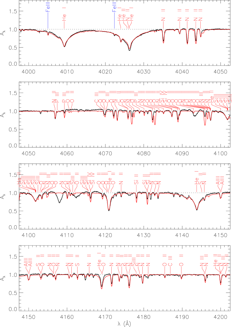
Figure B.17: (a) The median Subaru spectrum of V652 Her between phases 0.60 and 0.70 (black), together with an approximate LTE synthetic spectrum computed using the parameters given in § 5.1 (red). Lines in the model with $W_{\lambda}>10$ mÅ are identified by ion. Ions with $Z>20$ are shown in blue. The hydrogen Balmer lines at 4101 Å and 4340 Å are not labelled but are included in the model. The model continuum is shown as a dotted line. Strong broad features around 4093, 4108, 4112 and 4126 Å  are instrumental artefacts.

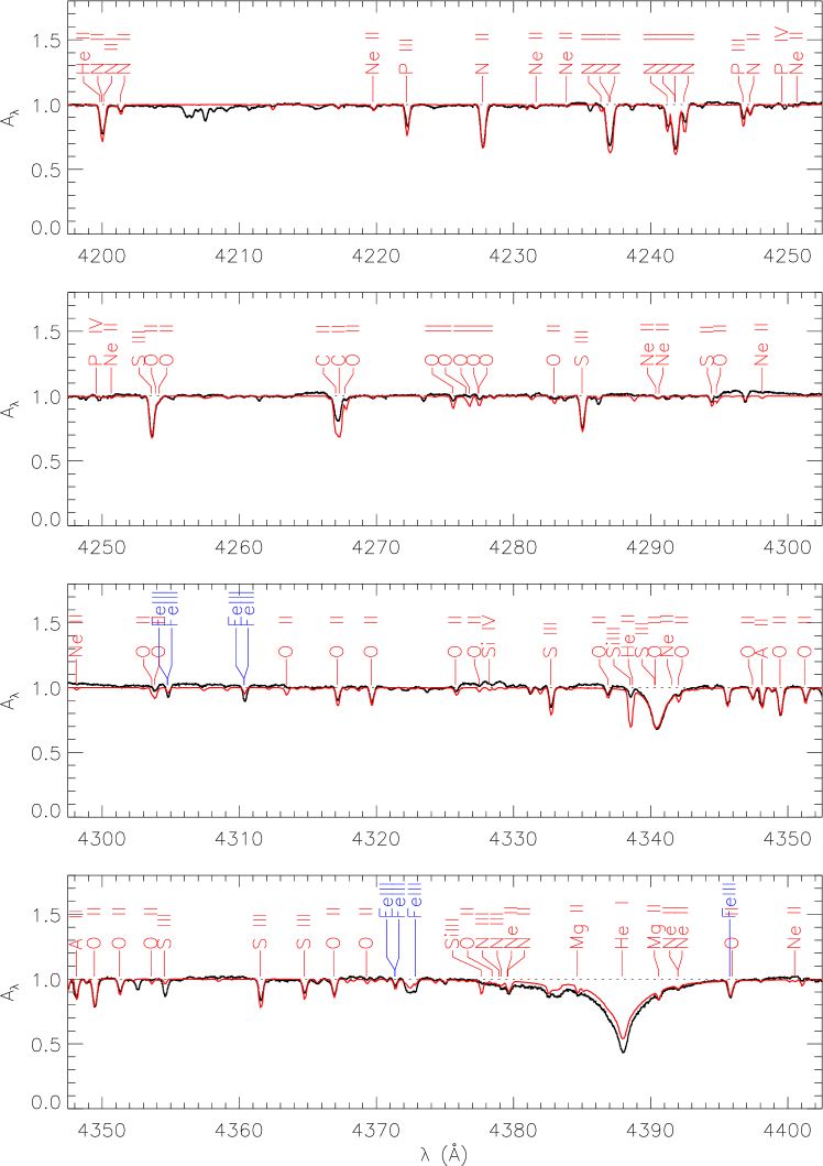
Figure B.17: (b) contd.

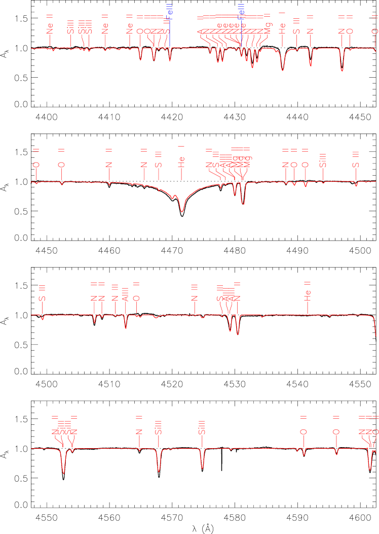
Figure B.17: (c) contd. Sharp features around 4578 and 4580 Å  are instrumental artefacts

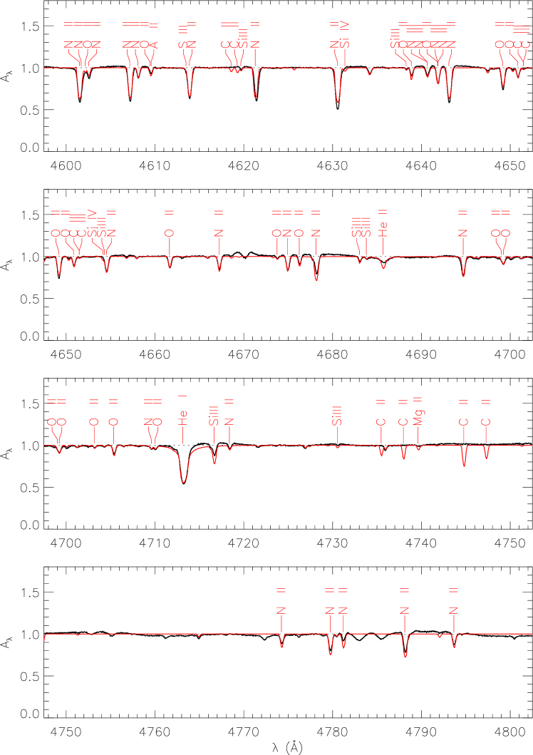
Figure B.17: (d) contd. Strong broad features around 4783 and 4786 Å  are instrumental artefacts.

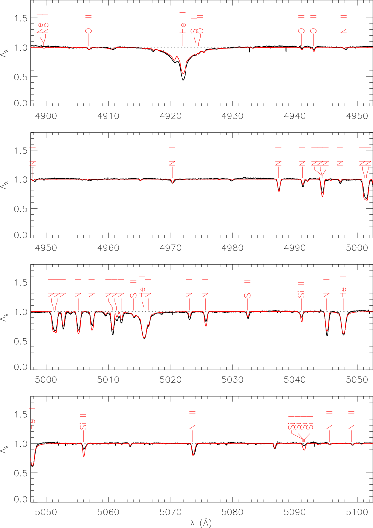
Figure B.17: (e) contd.

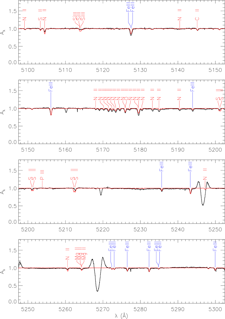
Figure B.17: (f) contd. Strong broad features around 5247 and 5268 Å  are instrumental artefacts.

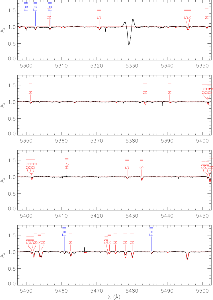
Figure B.17: (g) contd. A strong broad feature at 5329 Å is an instrumental artefacts.

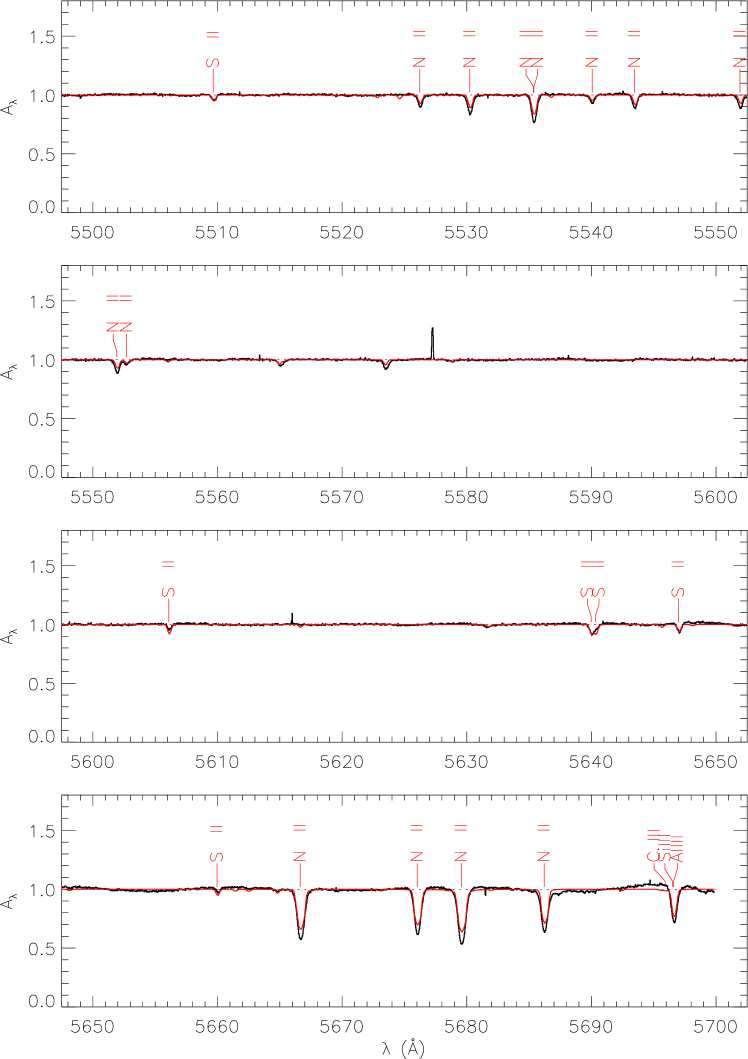
Figure B.17: (h) contd. An emission feature at 5577 Å is a cosmic ray hit.

References

- Baade (1926) Baade W., 1926, Astron. Nachr., 228, 359
- Ballester (1994) Ballester P., 1994, A&A, 286, 1011
- Barnard et al. (1969) Barnard A. J., Cooper J., Shamey L. J., 1969, A&A, 1, 28
- Behara & Jeffery (2006) Behara N. T., Jeffery C. S., 2006, A&A, 451, 643
- Berger & Greenstein (1963) Berger J., Greenstein J. L., 1963, PASP, 75, 336
- Brown et al. (2001) Brown T. M., Sweigart A. V., Lanz T., Landsman W. B., Hubeny I., 2001, ApJ, 562, 368
- Castor (1968) Castor J. I., 1968, ApJ, 154, 793
- Fadeyev & Lynas-Gray (1996) Fadeyev Y. A., Lynas-Gray A. E., 1996, MNRAS, 280, 427
- Gehrels et al. (2004) Gehrels N., Chincarini G., Giommi P., Mason K. O., Nousek J. A., Wells A. A., White N. E., Barthelmy S. D., 2004, ApJ, 611, 1005
- Hill et al. (1981) Hill P. W., Kilkenny D., Schönberner D., Walker H. J., 1981, MNRAS, 197, 81
- Jeffery (1984) Jeffery C. S., 1984, MNRAS, 210, 731
- Jeffery (2008) Jeffery C. S., 2008, Comm. Asteroseismol., 157, 240
- Jeffery & Hill (1986) Jeffery C. S., Hill P. W., 1986, MNRAS, 221, 975
- Jeffery et al. (1999) Jeffery C. S., Hill P. W., Heber U., 1999, A&A, 346, 491
- Jeffery et al. (2001) Jeffery C. S., Woolf V. M., Pollacco D. L., 2001, A&A, 376, 497
- Kilkenny (1988) Kilkenny D., 1988, MNRAS, 232, 377
- Kilkenny et al. (2005) Kilkenny D., Crause L. A., van Wyk F., 2005, MNRAS, 361, 559
- Kilkenny & Lynas-Gray (1982) Kilkenny D., Lynas-Gray A. E., 1982, MNRAS, 198, 873
- Kilkenny & Lynas-Gray (1984) Kilkenny D., Lynas-Gray A. E., 1984, MNRAS, 208, 673
- Kilkenny et al. (1996) Kilkenny D., Lynas-Gray A. E., Roberts G., 1996, MNRAS, 283, 1349
- Kilkenny & Marang (1991) Kilkenny D., Marang F., 1991, Inf. Bull. Var. Stars, 3660, 1
- Kukarkin et al. (1977) Kukarkin B. V., Kholopov P. N., Fedorovich V. P., Kireyeva N. N., Kukarkina N. P., Medvedeva G. I., Perova N. B., 1977, Inf. Bull. Var. Stars, 1248, 1
- Landolt (1975) Landolt A. U., 1975, ApJ, 196, 789
- Lynas-Gray et al. (1984) Lynas-Gray A. E., Schönberner D., Hill P. W., Heber U., 1984, MNRAS, 209, 387
- McCormac & et al. (2014) McCormac J., Pollacco D., NGTS Consortium, 2014, Rev. Mex A&A (Ser. Conf.), 45, 98
- Montañés Rodriguez & Jeffery (2001) Montañés Rodriguez P., Jeffery C. S., 2001, A&A, 375, 411
- Montañés Rodríguez & Jeffery (2002) Montañés Rodríguez P., Jeffery C. S., 2002, MNRAS, 384, 433
- Noguchi et al. (2002) Noguchi K., Aoki W., Kawanomoto S., Ando H., Honda S., Izumiura H., Kambe E., Okita K., Sadakane K., Sato B., Tajitsu A., Takada-Hidai T., Tanaka W., Watanabe E., Yoshida M., 2002, PASJ, 54, 855
- Page et al. (2013) Page M. J., Kuin N. P. M., Breeveld A. A., Hancock B., Holland S. T., Marshall F. E., Oates S., Roming P. W. A., Siegel M. H., Smith P. J., Carter M., De Pasquale M., Symeonidis M., Yershov V., Beardmore A. P., 2013, MNRAS, 436, 1684
- Parsons (1972) Parsons S. B., 1972, ApJ, 174, 57
- Przybilla et al. (2005) Przybilla N., Butler K., Heber U., Jeffery C. S., 2005, A&A, 443, L25
- Rogers & Iglesias (1992) Rogers F. J., Iglesias C. A., 1992, ApJS, 79, 507
- Saio (1986) Saio H., 1986, MNRAS, 221, 1P
- Saio (1993) Saio H., 1993, MNRAS, 260, 465
- Saio & Jeffery (1988) Saio H., Jeffery C. S., 1988, ApJ, 328, 714
- Saio & Jeffery (2000) Saio H., Jeffery C. S., 2000, MNRAS, 313, 671
- Seaton et al. (1994) Seaton M. J., Yan Y., Mihalas D., Pradhan A. K., 1994, MNRAS, 266, 805
- Shapley (1914) Shapley H., 1914, ApJ, 40, 448
- Stetson (1987) Stetson P. B., 1987, PASP, 99, 191
- Szabó et al. (2007) Szabó R., Buchler J. R., Bartee J., 2007, ApJ, 667, 1150
- Wesselink (1946) Wesselink A. J., 1946, Bull. Astron. Inst. Netherlands, 10, 91
- Zhang & Jeffery (2012) Zhang X., Jeffery C. S., 2012, MNRAS, 419, 452