Fast and accurate determination of modularity and its effect size

Abstract

We present a fast spectral algorithm for community detection in complex networks. Our method searches for the partition with the maximum value of the modularity via the interplay of several refinement steps that include both agglomoration and division. We validate the accuracy of the algorithm by applying it to several real-world benchmark networks. On all these, our algorithm performs as well or better than any other known polynomial scheme. This allows us to extensively study the modularity distribution in ensembles of Erdős-Rényi networks, producing theoretical predictions for means and variances inclusive of finite-size corrections. Our work provides a way to accurately estimate the effect size of modularity, providing a $z$-score measure of it and enabling a more informative comparison of networks with different numbers of nodes and links.

1 Introduction

Networked systems, in which the elements of a set of nodes are linked in pairs if they share a common property, often feature complex structures extending across several length scales. At the lowest length scale, the number of links of a node defines its degree $k$. At the immediately higher level, the links amongst the neighbours of a node define the structure of a local neighbourhood. The nodes in some local neighbourhoods can be more densely linked amongst themselves than they are with nodes belonging to other neighbourhoods. In this case, we refer to these densely connected modules as communities. A commonly used indicator of the prominence of community structure in a complex network is its maximum modularity $Q$. Given a partition of the nodes into modules, the modularity measures the difference between its intra-community connection density and that of a random graph null model [1, 2, 3, 4]. Highly modular structures have been found in systems of diverse nature, including the World Wide Web, the Internet, social networks, food webs, biological networks, sexual contacts networks, and social network formation games [5, 6, 7, 8, 9, 10, 11, 12, 13, 14]. In all these real-world systems, the communities correspond to actual functional units. For instance, communities in the WWW consist of web pages with related topics, while communities in metabolic networks relate to pathways and cycles [7, 12, 15, 16]. A modular structure can also influence the dynamical processes supported by a network, affecting synchronization behaviour, percolation properties and the spreading of epidemics [17, 18, 19]. The development of methods to detect the community structure of complex systems is thus a central topic to understand the physics of complex networks [20, 21, 22, 23, 24].

However, the use of modularity maximization to find communities in networks presents some challenges and issues. The principal challenge is that finding the network partition that maximizes the modularity is an NP-hard computational problem [25]. Therefore, for a practical application, it is important to find a fast algorithm that produces an accurate estimate of the maximum modularity of any given network. Among the issues is that, in general, modularity itself does not allow for the quantitative comparison of the modular structure between different networks. For networks with the same number of nodes and links, a higher modularity does indicate a more modular network structure. However, this is not necessarily the case when networks with different number of nodes or links are compared. In this paper, we present a spectral algorithm for community detection based on modularity maximization and introduce a method to estimate the effect size of modularity. The algorithm we present incorporates both variations of the Kernighan-Lin algorithm that remove constraints imposed on the resulting partition and an agglomeration step that can combine communities. We validate the accuracy of our algorithm, which always terminates in polynomial time, by applying it to a set of commonly studied real-world example networks. We find that no other currently known fast modularity maximizing algorithm performs better on any network studied. We also use our algorithm to perform an extensive numerical study of the distribution of modularity in ensembles of Erdős-Rényi networks. Then, using our numerical results, we fit finite-size corrections to theoretical predictions previously derived for the mean of the distribution [26, 27, 28] and to the novel expression we derive for the variance, both of which are valid in the large network limit. Finally, considering Erdős-Rényi networks as a null-model, we obtain an analytic expression for a $z$-score measure of the effect-size of modularity that is accurate for networks of any size that have an average degree of 1 or more. A quantitative comparison of $z$-scores can be used to complement that of the modularities of different networks, including those with different numbers of nodes and/or links.

2 Modularity and effect size

Given a network with $N$ nodes and $m$ links, one can define a partition of the nodes by grouping them into communities. Let $c_{i}$ indicate the community to which node $i$ is assigned, and let $\left\{c\right\}$ be the set of communities into which the network was partitioned. Then, the modularity $q$ of the partition is

$$q_{\left\{c\right\}}=\frac{1}{2m}{\sum}_{ij}\left(A_{ij}-\frac{k_{i}k_{j}}{2m}\right)\delta_{c_{i},c_{j}}\>,$$ (1)

where $k_{i}$ is the degree of node $i$, and $A$ is the adjacency matrix, whose $\left(i,j\right)$ element is 1 if nodes $i$ and $j$ are linked, and 0 otherwise. With this definition, the value of $q$ is larger for partitions where the number of links within communities is larger than what would be expected based on the degrees of the nodes involved [29]. Of course, even in the case of a network with quite a well-defined community structure, it is usually possible to define a partition with a small modularity. For instance, one can artificially split the network into modules consisting of pairs of unconnected nodes taken from different actual communities (see Fig. 1). Thus, in order to properly characterize the community structure it is instead necessary to find the particular partition $\left\{C\right\}$ that maximizes the modularity,

$$\left\{C\right\}=\arg\max_{\left\{c\right\}}\left\{q_{\left\{c\right\}}\right\}\>.$$

Henceforth, we indicate with $Q$ the maximum modularity of a network, which is the modularity of the partition $\left\{C\right\}$:

$$Q=q_{\left\{C\right\}}=\max_{\left\{c\right\}}\left\{q_{\left\{c\right\}}\right\}=\max_{\left\{c\right\}}\left\{\frac{1}{2m}{\sum}_{ij}\left(A_{ij}-\frac{k_{i}k_{j}}{2m}\right)\delta_{c_{i},c_{j}}\right\}\>.$$

The maximum modularity $Q$ corresponds to the particular partition of the network that divides it into the most tightly bound communities. However, simply finding this partition is not sufficient to determine the statistical importance of the community structure found.

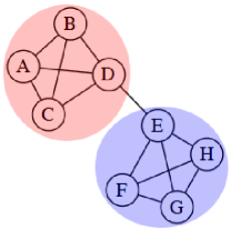
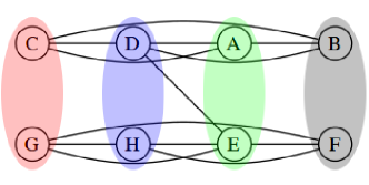
Figure 1: Different partitions of the same network. The partition on the left divides the network into two communities with densely connected nodes. The partition on the right divides the same network into modules consisting of disconnected nodes, resulting in a low value of the modularity.

To see this, consider an ensemble of random graphs with a fixed number of nodes $N$ and a fixed number of links $m$. As these networks are random, one can safely say that they have no real communities. Then, one could assume a vanishing average modularity $\left\langle q\right\rangle_{\left\{c\right\}}$ on the ensemble. However, the amount of community structure is quantified by the extremal measure $Q$, rather than $\left\langle q\right\rangle_{\left\{c\right\}}$. Thus, one cannot exclude a priori the existence of a partition with non-zero modularity even on a completely random graph. This implies that one can attach a fuller meaning to the maximum modularity of a given network by comparing it to the expected maximum modularity of an appropriate set of random graphs. Then, the comparison defines an effect size for the modularity, measuring the statistical significance of a certain observed $Q$. Of course, the random graph ensemble must be appropriately chosen to represent a randomized version of the network analyzed.

A suitable random graph set for this study is given by the Erdős-Rényi (ER) model ${\cal G}\left(N,p\right)$ [30]. In the model, links between any pair of nodes exist independently with fixed probability $p$. As there is no other constraint imposed, ER graphs are completely random, which makes them a natural choice for a null model. Of course, it is conceivable that another null model could be used for specific types of networks. In this case, one could generate random ensembles of networks with a specified set of constraints, using appropriate methods such as degree-based graph construction [31, 32]. To find the correct probability to use, we require that the expected number of links in each individual graph must equal the number of links in the network we are studying. The expected number of links in an Erdős-Rényi network with $N$ nodes is

$$\left\langle m\right\rangle=\frac{pN\left(N-1\right)}{2}\>.$$

Thus, the probability of connection must be

$$p=\frac{2m}{N\left(N-1\right)}\>.$$ (2)

Then, we can compare $Q$ with the expected maximum modularity $\left\langle Q_{ER}\right\rangle$ of the ER ensemble thus defined. One simple way to perform the comparison is calculating the difference between $Q$ and $\left\langle Q_{ER}\right\rangle$. However, while this approach provides a certain estimate of the importance of $Q$, it is not entirely satisfactory. In fact, the same difference acquires more or less significance depending on the width of the distribution of $\left\langle Q_{ER}\right\rangle$. Then, it is a natural choice to normalize the difference between maximum modularities dividing it by the standard deviation $\sigma_{ER}$ of $\left\langle Q_{ER}\right\rangle$

$$z=\frac{Q-\left\langle Q_{ER}\right\rangle}{\sigma_{ER}}\>.$$ (3)

The equation above defines a particular measure of the effect size of $Q$ called $z$-score. Positive $z$-scores indicate more modular structure than expected in a random network, while negative $z$-scores indicate less modular structure than expected in a random network.

3 Algorithm

To find the maximum modularity partition of a network, we introduce a variation of the leading eigenvector method [29, 33]. The full algorithm provides a best guess of the maximum modularity partition by progressively refining the community structure. The general idea is as follows. In the beginning, all the nodes of the network are in the same community. Then, one introduces the simplest possible division, by splitting the network into two different modules. The choice of the nodes to assign to either module is refined by several steps that are described in detail below, and the whole process is then repeated on each single community until no improvement in modularity can be obtained. A summary of the entire algorithm is given in Subsection 3.5.

3.1 Bisection

The first step in the algorithm consists of the bisection of an existing community. To find the best bisection, we exploit the spectral properties of the modularity matrix $B$, whose elements are defined by

$$B_{ij}=A_{ij}-\frac{k_{i}k_{j}}{2m}\>.$$

Substituting this into Eq. 1, we obtain an expression for the modularity of a partition in terms of $B$:

$$q_{\left\{c\right\}}=\frac{1}{2m}{\sum}_{ij}B_{ij}\delta_{c_{i},c_{j}}\>.$$ (4)

As we are considering splitting a community into two, we can represent any particular bisection choice by means of a vector $s$ whose element $s_{i}$ is $-1$ if node $i$ is assigned to the first community, and $1$ if it is assigned to the second. Then, using $\delta_{c_{i},c_{j}}=\frac{1}{2}\left(s_{i}s_{j}+1\right)$, Eq. 4 becomes

$$q_{\left\{c\right\}}=\frac{1}{4m}{\sum}_{ij}B_{ij}s_{i}s_{j}\>.$$ (5)

We can now express $s$ as a linear combination of the normalized eigenvectors $v$ of $B$

$$s=\sum_{i=1}^{N}\alpha_{i}v_{i}\>,$$

so that Eq. 5 becomes

$$q_{\left\{c\right\}}=\frac{1}{4m}\sum_{i=1}^{N}\alpha_{i}^{2}\lambda_{i}\>,$$ (6)

where $\lambda_{i}$ is the eigenvalue of $B$ corresponding to the eigenvector $v_{i}$. From Eq. 6, it is clear that to maximize the modularity one could simply choose $s$ to be parallel to the eigenvector $v_{1}$ corresponding to the largest positive eigenvalue $\lambda_{1}$. However, this approach is in general not possible, since the elements of $s$ are constrained to be either 0 or 1. Then, the best choice becomes to construct a vector $s$ that is as parallel as possible to $v_{1}$. To do so, impose that the element $s_{i}$ be 1 if ${v_{1}}_{i}$ is positive and $-1$ if ${v_{1}}_{i}$ is negative.

This shows that the whole bisection step consists effectively just of the search for the eigenvalue $\lambda_{1}$ and its corresponding eigenvctor $v_{1}$. As the modularity matrix $B$ is real and symmetric, this is easily found. For instance, one can use the well-known power method, or any of other more advanced techniques. If $\lambda_{1}>0$, we build our best partition as described above and compute the change in modularity $\Delta Q$; conversely, if $\lambda_{1}\leqslant 0$, we leave the community as is.

The computational complexity of the bisection step depends on the method used to find $\lambda_{1}$. In the case of the power method, it is ${\cal O}\left(Nm\right)$.

3.2 Fine tuning

Each bisection can often be improved using a variant of the Kernighan-Lin partitioning algorithm [34]. The algorithm considers moving each node $k$ from the community to which it was assigned into the other, and records the changes in modularity $\Delta Q^{\prime}\left(k\right)$ that would result from the move. Then, the move with the largest $\Delta Q^{\prime}\left(k\right)$ is accepted. The procedure is repeated $N$ times, each time excluding from consideration the nodes that have been moved at a previous pass. Effectively, this tuning step traverses a decisional tree in which each branching corresponds to one node switching community. The particular path taken along the tree is determined by choosing at each level the branch that maximizes $\Delta Q^{\prime}\left(k\right)$. Thus, it is clear that at each level $i$ in the tree the total modularity change $\Delta Q^{\prime}_{i}$ is simply the sum of the $\Delta Q^{\prime}\left(k\right)$ considered up to that point. When the process is over, and all the nodes have been eventually moved, one finds the level $i^{\ast}$ with the maximum total modularity change:

$$i^{\ast}=\arg\max_{i}\left\{\Delta Q^{\prime}_{i}\right\}\>.$$

If $\Delta Q^{\prime}_{i^{\ast}}$ is positive, the partition is updated by switching the community assignment for all the nodes corresponding to the branches taken along the path from level 1 to $i^{\ast}$; if, instead, $\Delta Q^{\prime}_{i^{\ast}}$ is negative or zero, the original partition obtained after the previous step is left unchanged. Finally, the entire procedure is repeated until it fails to produce an increase in total modularity.

In A, we detail an efficient implementation for this step, with a computational complexity of ${\cal O}(N^{2})$ per update.

3.3 Final tuning

After the bisection of a module, the nodes are assigned to two disjoint subsets. If the algorithm consisted solely of these steps, the only possible refinements to the community structure would be further division of these subsets. As a result, the separation of two nodes into two different communities would be permanent: once two nodes are separated, they can never again be found together in the same community. This kind of network partition has been proved to introduce biases in the results [35]. To avoid this, we introduce in our algorithm a “final tuning” step, that extends the local scope of the search performed by the fine tuning [35, 23, 24].

To perform this step, we work on the network after all communities have undergone the bisection and fine tuning steps individually. Then, we consider moving each node from its current community to all other existing communities, as well as moving it into a new community on its own. For each potential move we compute the corresponding change in modularity $\Delta Q^{\prime\prime}\left(k,\alpha\right)$, where $k$ is the node being analyzed, and $\alpha$ is the target community. The particular move yielding the largest $\Delta Q^{\prime\prime}$ is then accepted. The procedure is repeated, each time not considering the nodes that have already been moved, until all the nodes have been reassigned to a different community. Similar to the fine tuning step, at the end of the process one looks at the decisional tree traversed to find the intermediate level $i^{\ast}$ with the largest total increase in modularity $\Delta Q^{\prime\prime}_{i^{\ast}}$. If this is positive, the network partition is updated by permanently accepting the node reassignments corresponding to the branches followed up to level $i^{\ast}$. Conversely, if $\Delta Q^{\prime\prime}_{i^{\ast}}$ is negative or zero, the starting network partition is retained. The whole procedure is then repeated until it does not produce any further increase in modularity.

In B, we detail an efficient implementation for this step, with a computational complexity of ${\cal O}(N^{3})$ per update.

3.4 Agglomeration

Both the fine tuning and the final tuning algorithms refine the best guess for the maximum modularity partition by performing local searches in modularity space. In other words, both tuning algorithms only consider moving individual nodes to improve the current partition. Here, we introduce a tuning step that performs a global search by considering moves involving entire communities. In particular, the new step tries to improve a current partition by merging pairs of communities.

A global search of this kind offers the possibility of finding partitions that would be inaccessible to a local approach. For example, assume that merging two communities would result in an increase of modularity. A local search could still be unable to find this new partition because the individual node moves could force it to go through partially merged states with lower modularity. If this modularity penalty is large enough, the corresponding moves will never be considered. Conversely, attempting to move whole communities allows to jump over possible modularity barriers in search for a better partition.

Thus, after each final tuning, we perform an agglomeration step as follows. First, we consider all existing communities and for each pair of communities $\alpha$ and $\beta$ we compute the change in modularity $\Delta Q^{\prime\prime\prime}\left(\alpha,\beta\right)$ that would result from their merger. Then, we merge the two communities yielding the largest $\Delta Q^{\prime\prime\prime}$. This process is repeated until only one community is left containing all the nodes. Then, we look at the decisional tree, as for the previous steps, and find the level $i^{\ast}$ corresponding to the largest total increase in modularity. If $\Delta Q^{\prime\prime\prime}_{i^{\ast}}$ is non-negative, we update the network partition by performing all the community mergers resulting in the intermediate configuration of the level $i^{\ast}$. If, instead, $\Delta Q^{\prime\prime\prime}$ is negative, the original partition is retained. Finally, the whole procedure is repeated until no further improvement can be obtained.

Note that in all the steps described we could encounter situations where more than one move yields the same maximum increase of modularity. In such cases we randomly extract one of the equivalent moves and accept it. The only exception is the determination of $i^{\ast}$ in the agglomeration step: if multiple levels of the decisional tree yield the same largest $\Delta Q^{\prime\prime\prime}$, rather than making a random choice, we pick the one with the lowest number of communities. This is intended to avoid spurious partitions of actual communities as could result from the previous steps.

In C, we detail an efficient implementation for this step, with a computational complexity of ${\cal O}(N^{3})$.

3.5 Summary of the algorithm

The steps described in the previous subsections can be put in an algorithmic form, yielding our complete method. Given a network of $N$ nodes:

1. Initialize the community structure with all the nodes partitioned into a single community.

2. Let $r$ be the current number of communities, and let $\alpha$ be a numerical label indicating which community we are working on. Set $\alpha=1$.

3. Attempt to bisect community $\alpha$ using the leading eigenvalue method, described in Subsection 3.1. Record the increase in modularity $\Delta Q$.

4. Perform a fine-tuning step, as described in Subsection 3.2. Record the increase in modularity $\Delta Q^{\prime}$.

5. If $\alpha<r$, increase $\alpha$ by 1 and go to step (iii).

6. Perform a final tuning step, as described in Subsection 3.3. Record the increase in modularity $\Delta Q^{\prime\prime}$.

7. Peform an agglomeration step as described in Subsection 3.4. Record the increase in modularity $\Delta Q^{\prime\prime\prime}$.

8. If the total increase in modularity $\Delta Q+\Delta Q^{\prime}+\Delta Q^{\prime\prime}+\Delta Q^{\prime\prime\prime}$ is positive, repeat from step (ii); otherwise, stop.

Note that one is free to arbitrially set the tolerances for each of the various numeric comparisons in the different steps of the algorithm. Every network will have a set of optimal tolerances, which can be empirically determined, that will yield the best results. Generally, these tolerances should not be too low, as they would make the algorithm behave like a hill climbing algorithm. At the same time, they should not be too high, as they would produce, effectively, a random search.

3.6 Algorithm validation

Table 1: Algorithm accuracy validation. The comparison between the maximum modularity found by our algorithm ($Q$) and the best published result ($Q_{\mathrm{pub}}$) shows that no other modularity maximizing scheme performs better than our method. The benchmark networks used are, in order, the social network in an American karate gym, the social network of a community of dolphins in New Zealand, the network of co-purchases of political books on Amazon.com in 2004, the word adjacency network in David Copperfield, a collaboration network between jazz musicians, the metabolic network in C. Elegans, the network of emails exchanged between members of the Universitat Rovira i Virgili in Tarragona, a network of trust in cryptographic key signing, and a symmetrized snapshot of the structure of the Internet at the level of autonomous systems, as of July 22, 2006. The “Time” column contains the time needed to complete a single run of the algorithm on a stand-alone affordable workstation at the time of writing. The last column contains references to the methods used to obtain the best result previously published for the corresponding network.

Network	Nodes	Links	$Q$	$z$-score		Time		$Q_{\mathrm{pub}}$	Method
Karate [36]	34	78	$0.4198$	1.	68	0.	45 ms	$0.4198$	[24, 37, 38, 39, 40]
Dolphins [41]	62	159	$0.5285$	5.	76	1.	39 ms	$0.5276$	[39]
Books [42]	105	441	$0.5272$	18.	27	2.	18 ms	$0.5272$	[24, 37, 39]
Words [29]	112	425	$0.3134$	-3.	51	5.	65 ms	$0.3051$	[24]
Jazz [43]	198	2742	$0.4454$	108.	91	16.	67 ms	$0.4454$	[24, 38]
C. Elegans [37]	453	2025	$0.4526$	21.	97	155.	85 ms	$0.4522$	[24, 35]
Emails [44]	1133	5045	$0.5827$	70.	89	1.	30 s	$0.5825$	[24]
PGP [45]	10680	24316	$0.884$	-144.	17	43.	33 min	$0.884$	[38]
Internet[46]	22963	48436	$0.6693$	-217.	95	4.	08 h	$0.6475$	[23]

To validate the accuracy of our algorithm, we applied it to a set of commonly studied real-world unweighted undirected benchmark networks, and compared its performance with the best result amongst known methods. The results are shown in Table 1. For each network we ran our algorithm a number of times, and the best result we obtained is what is reported in the Table. In each case, the best result was obtained within the first one hundred runs. For the time estimates, we ran our algorithm on a single core of an affordable, stand-alone workstation with a single Intel^® Core^™ i5-2400 CPU and 4 GB of RAM. The processor is, at the time of writing, almost 4 years old, having been introduced by the manufacturer in January 2011. In all cases considered, no other fast modularity maximizing algorithm finds a more modular network partition than the one identified by our method. In fact, there are no reported results even from simulated annealing, a slow algorithm, that exceed ours.

4 Estimating the effect size

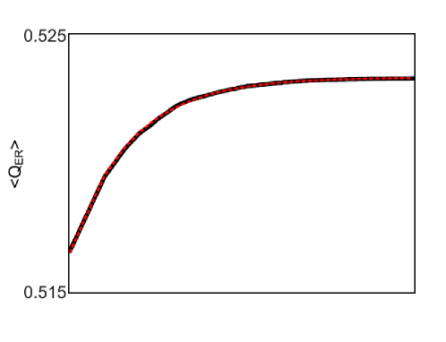
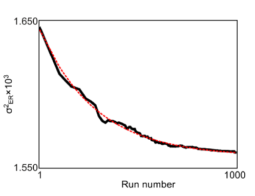
Figure 2: Convergence of modularity distribution for an ensemble of ER graphs with $N=50$ and $p=0.06$. The top panel shows the best modularity measured after a given number of runs; the bottom panel shows the respective variance. The dashed red lines are power-law fits to the measured data.

As discussed in Section 2, to compute the $z$-score for a given partition of a network, we need to know the expected maximum modularity $\left\langle Q_{ER}\right\rangle$ of an appropriately defined ER ensemble, and its standard deviation $\sigma_{ER}$. To find an expression for these quentities, we start from the results in Refs. [26, 27, 28], which provide an estimate of $\left\langle Q_{ER}\right\rangle$ for a generic ER ensemble ${\cal G}\left(N,p\right)$:

$$\left\langle Q_{ER}\right\rangle=0.97\sqrt{\frac{1-p}{Np}}\>.$$ (7)

However, the equation above was derived under the assumptions that $N\gg 1$ and $p\sim 1$. In other words, the estimate is expected to be valid for large dense networks. Nevertheless, in many real-world systems, networks are typically sparse [47], and often their size is only few tens of nodes [36, 41, 43]. Therefore, to ensure the applicability of Eq. 7, it is necessary to find appropriate scaling corrections. Finding such corrections analytically is a very difficult problem. Thus, here we employ a numerical approach.

First of all, to measure $\left\langle Q_{ER}\right\rangle$ and $\sigma_{ER}$, we performed extensive numerical simulations, generating ensembles of Erdős-Rényi random graphs with $N$ between 10 and 1000 and $p$ between $1/N$ and 1. Then, we applied the algorithm described in Section 3 to each network in each ensemble. However, as we discussed before, the algorithm incorporates several elements of randomness. In principle it can give a different result every time it is run. Thus, to estimate the expected maximum modularity for each choice of $N$ and $p$, we ran the algorithm 1000 times on each network, recording after each run $r$ the largest value of modularity obtained thus far, and computed ensemble averages of $\left\langle Q_{ER}\right\rangle\left(r\right)$ and $\sigma^{2}_{ER}\left(r\right)$. The results show a fast convergence of the quantities to their asymptotic value. To model this convergence, we postulate that the difference between the observed value and the asymptotic one decays like a power-law with the number of runs $r$:

$$\left\langle Q_{ER}\right\rangle\left(r\right) =\left\langle Q_{ER}\right\rangle-Ar^{-B}\>,$$

$$\sigma^{2}_{ER}\left(r\right) =\sigma^{2}_{ER}-Cr^{-D}\>.$$

We can then fit the curves using $A$, $B$, $C$, $D$, $\left\langle Q_{ER}\right\rangle$ and $\sigma^{2}_{ER}$ as fit parameters, as shown in Fig. 2, obtaining our estimate for the asymptotic values. In all cases studied, we find that the distribution of modularity values is approximately Gaussian.

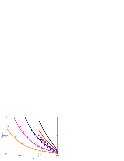
Figure 3: Expected maximum modularity for ER ensembles. The numerical data for $N=10$ (black dots), 20 (red squares), 50 (blue diamonds), 200 (pink triangles) and 1000 (orange stars) show that the predictions of Eq. 7 (like-coloured lines) are accurate mostly for large dense networks.

Figure 3 shows the final numerical results for $\left\langle Q_{ER}\right\rangle$, with the predictions of Eq. 7 for comparison. For small system sizes, the measured modularity is lower than that its theoretical prediction. For larger systems, however, the approximation is effectively in agreement with simulations, expect for lower values of $p$, in the vicinity of the giant component transition. This suggests the correction we need is twofold, consisting of a multiplicative piece to scale down the prediction for small systems, and an additive piece to account for the case of sparse networks. Thus, an Ansatz for the corrected form is

$$\left\langle Q_{ER}\right\rangle=C_{1}\cdot 0.97\sqrt{\frac{1-p}{Np}}+C_{2}\>.$$ (8)

The simulation results seem to quickly approach the prediction of Eq. 7 with increasing system size. Therefore, we assume that $C_{1}$ is of the form

$$C_{1}=1-\lambda\mathrm{e}^{-\frac{N}{N_{0}}}\>.$$

Fitting these two parameters with the high-$p$ tail of the results yields

$$\lambda =\frac{7}{5}\>,$$

$$N_{0} =50\>$$

Therefore, the multiplicative correction is

$$C_{1}=1-\frac{7}{5}\mathrm{e}^{-\frac{N}{50}}\>.$$ (9)

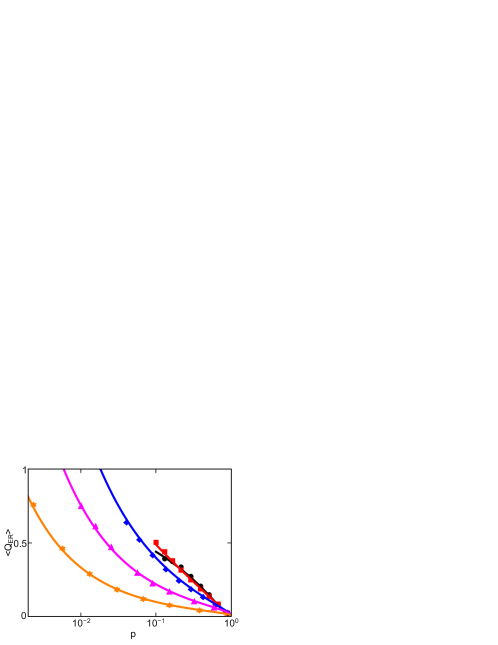
Figure 4: Scaling corrections for expected maximum modularity. The predictions of Eq. 12 are accurate throughout the range of $p$, and for all system sizes. The numerical data shown are for $N=10$ (black dots), 20 (red squares), 50 (blue diamonds), 200 (pink triangles) and 1000 (orange stars).

The additive piece of the correction clearly depends on $p$ and $N$. Thus, we start by assuming the general form

$$C_{2}=C_{0}p^{\alpha}\left(1-p\right)^{\beta}N^{\gamma}\>,$$ (10)

where the exponents $\alpha$, $\beta$, and $\gamma$ may depend on $N$. Fitting these parameters yields

$$C_{0} =1$$

$$\alpha =-\frac{1}{6}\log\left(\frac{2}{5}N\right)$$

$$\beta =\frac{5}{4}$$

$$\gamma =-\frac{6}{5}+\frac{13}{15}\mathrm{e}^{-\frac{N}{100}}\>.$$

To obtain the corrected expression for the expected maximum modularity, substitute the parameter values into Eq. 10, then substitute Eq. 10 and Eq. 9 into Eq. 8:

$$\left\langle Q_{ER}\right\rangle=\left(1-\frac{7}{5}\mathrm{e}^{-\frac{N}{50}}\right)0.97\sqrt{\frac{1-p}{Np}}+p^{-\frac{1}{6}\log{\left(\frac{2}{5}N\right)}}\left(1-p\right)^{\frac{5}{4}}N^{-\frac{6}{5}+\frac{13}{15}\mathrm{e}^{-\frac{N}{100}}}.$$ (12)

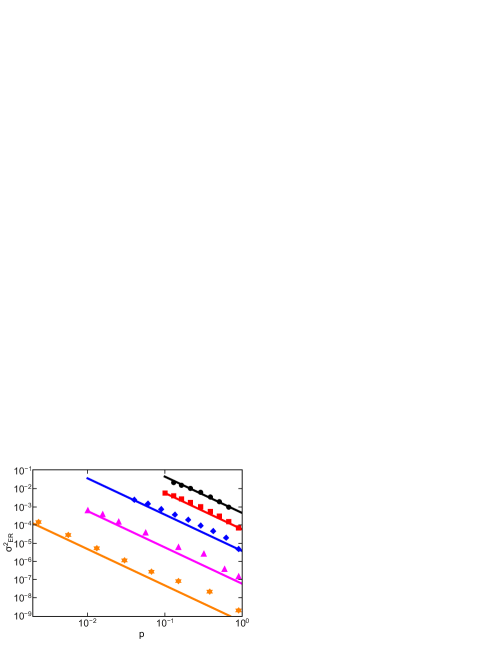
Figure 5: Variance of the expected maximum modularity for ER ensembles. The numerical data for $N=10$ (black dots), 20 (red squares), 50 (blue diamonds), 200 (pink triangles) and 1000 (orange stars) show that the predictions of Eq. 17 (like-coloured lines) are accurate mostly for small sparse networks.

The predictions of Eq. 12, shown in Fig. 4, show a very good agreement for all system sizes and all values of $p$. However, to compute the $z$-score of a given modularity measurement on a particular network, we need to be able to express also the variance of the modularity in the null model of choice. To do so, we first use Eq. 7 to find the expected form of the variance, using propagation of uncertainties. Notice, however, that Eq. 7 was originally derived in the framework of the ${\cal G}\left(N,m\right)$ ensemble, in which the number of nodes $N$ and the number of edges $m$ are held fixed, rather than in the ${\cal G}\left(N,p\right)$ ensemble. Therefore, in finding an equation for the variance of $\left\langle Q_{ER}\right\rangle$, $p$ cannot be considered constant. Then,

$$\sigma^{2}_{\left\langle Q_{ER}\right\rangle}=\left(\partial_{p}\left\langle Q_{ER}\right\rangle\right)^{2}\sigma^{2}_{p}\>.$$ (13)

With $m$ fixed, one can write $p=\frac{2m}{N^{2}}$, hence

$$\sigma_{p}^{2}=\left(\partial_{m}p\right)^{2}\sigma^{2}_{m}=\frac{4}{N^{4}}\sigma^{2}_{m}\>.$$ (14)

As $m$ is binomially distributed, its variance is

$$\sigma^{2}_{m}=\frac{N^{2}}{2}p\left(1-p\right)\>.$$ (15)

Substituting Eq. 15 into Eq. 14 yields

$$\sigma_{p}^{2}=\frac{2}{N}p\left(1-p\right)\>.$$ (16)

Finally, substituting Eq. 16 into Eq. 13 one obtains

$$\sigma^{2}_{\left\langle Q_{ER}\right\rangle}=\frac{0.97^{2}}{2}\frac{1}{N^{3}p^{2}}\>.$$ (17)

Once more, the results of the numerical simulations, shown in Fig. 5, indicate that the actual variance deviates from the theoretical prediction. Thus, also in this case we need to find a correction. The deviation of the measured variances from those predicted by means of Eq. 17 rapidly increases with the size of the network, apparently converging towards a constant. Therefore, we postulate that the correction $C^{\prime}$ to Eq. 17 is multiplicative and has the form

$$C^{\prime}=C^{\prime}_{0}-\mathrm{e}^{-\varepsilon\left(N-N_{0}\right)}\>.$$

A fit of these parameters gives $C^{\prime}_{0}=2$, $\varepsilon=\frac{1}{50}$ and $N_{0}=10$. Thus, the final expression for the variance of the expected maximum modularity in a ${\cal G}\left(N,p\right)$ Erdős-Rényi ensemble is

$$\sigma^{2}_{\left\langle Q_{ER}\right\rangle}=\left(2-\mathrm{e}^{-\left(N-10\right)/50}\right)\frac{0.97^{2}}{2}\frac{1}{N^{3}p^{2}}\>.$$ (18)

Again, the predictions of Eq. 18, shown in Fig. 6, are in very good agreement with the numerical simulations. We note, however, that for values of $p$ greater than approximately $0.15$ the numerically measured variance deviates slightly from the predicted behaviour. In this region, we appear to slightly overestimate the magnitude of the $z$-score. We postulate, however, that this is due to an increased hardness in finding the best partition for networks having this range of connectivity. Assuming this is case and our prediction of the variance is correct in this region, our estimate of the magnitude of the $z$-score is accurate throughout the range.

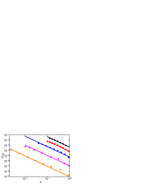
Figure 6: Scaling corrections for variance of expected maximum modularity. The predictions of Eq. 18 represent a substantial improvement for any $p$ and all system sizes. The numerical data shown are for $N=10$ (black dots), 20 (red squares), 50 (blue diamonds), 200 (pink triangles) and 1000 (orange stars).

With the corrections we developed, it is finally possible to compute the $z$-score of a modularity measurement on any particular network. First, one determines $p$ using Eq. 2. Then, one uses Eqs. 12 and 18, to calculate $\left\langle Q_{ER}\right\rangle$ and $\sigma_{ER}$, respectively. Finally, using these values, Eq. 3 yields the $z$-score.

To further motivate the choice of the Erdős-Rényi random graph ensemble as the natural null model for network partitioning, we used the degree-based graph sampling algorithm of Ref. [31] to construct ensembles of networks with the same degree sequences (SDS) as the benchmark systems we used for validation. The comparison between the $z$-scores obtained with the two approaches is shown in Table 2. In all cases, the SDS $z$-scores are more positive than the ER ones. This strongly suggests that the SDS ensemble underestimates the expected maximum modularity. The reason for this behaviour is in the term $-\frac{k_{i}k_{j}}{2m}$ in Eq. 1, which estimates the number of links between a node of degree $k_{i}$ and one of degree $k_{j}$. This factor implicitly accounts for the possibility of multiple edges in the networks, and therefore its magnitude is larger than it should be. While this overestimate is negligible for ER graphs, it becomes significant for networks with degree distributions different from those of random graphs. The effect is particularly marked on scale-free networks, such as most of the ones we analyzed here, since random networks with a power-law degree distribution are known to be disassortative [48, 49]. These considerations suggest that the ER ensemble is the correct null model to use for the calculation of $z$-scores for modularity-based algorithms in most community detection applications.

Table 2: Null model motivation. Adopting as the null model the ensemble of networks with the same degree sequence (SDS) as the one studied always results in a more positive $z$-score, indicating an underestimation of the expected maximum modularity in the SDS ensemble. The networks used here are the same we used for the results shown in Table 1.

• Network	Nodes	Links	ER $z$-score		SDS $z$-score
  Karate [36]	34	78	1.	68	8.	06
  Dolphins [41]	62	159	5.	76	14.	85
  Books [42]	105	441	18.	27	37.	70
  Words [29]	112	425	-3.	51	2.	07
  Jazz [43]	198	2742	108.	91	150.	20
  C. Elegans [37]	453	2025	21.	97	238.	00
  Emails [44]	1133	5045	70.	89	177.	93
  PGP [45]	10680	24316	-144.	17	326.	00
  Internet[46]	22963	48436	-217.	95	358.	52

5 Conclusions

In this paper we have presented practical methods for identifying community structure in complex networks and for quantifying whether that structure is significant compared to what is expected in Erdős-Rényi networks. As such, our methods directly address the principal challenge and a major issue with using modularity maximization to identify a network’s community structure. In particular, we have presented the best of any currently known algorithm for finding the network partition that maximizes modularity. Then, making use of this algorithm and both existing and novel analytical results, we found analytic expressions for the mean and standard deviation of the distribution of modularity of ensembles of Erdős-Rényi networks. Using these expressions, which apply to all network sizes $N$ with average connectivity $p>1/N$, we have obtained an analytic transformation from modularity value to a $z$-score that measures the effect size of modularity.

The conversion from modularity value to the $z$-score of modularity effect size we have established is particularly noteworthy. Because of it, for the first time, one can easily estimate the relative importance of the modular structure in networks with different numbers of nodes or links. This allows a new form of comparative network analysis. For example, Table 1 lists the modularity $z$-scores of the real-world test networks we used to validate our algorithm. Note that most of the networks have a $z$-score much greater than 1, and thus their structure is substantially unlikely to be due to a random fluctuation, with the collaboration network of Jazz musicians being by far the least random of those studied. However, the Key Signing network has a large negative $z$-score. Thus, it is substantially less modular than a comparable ER network. This indicates that, even though the network has a very prominent modular structure, as evidenced by the large modularity, its links are nonetheless much more evenly distributed than expected if it were random. Similarly, we can say that the word adjacency network in “David Copperfield” has a slightly less modular structure than expected if random, and the Karate Club network has a modular structure that could still be attributed to a random fluctuation, although with a probability of only about 5%. This form of analysis is clearly much more informative than one that considers modularity alone. The difference is particularly striking, for instance, with the Key Signing network, which has a very high value of modularity, but a much less modular structure than a comparable random network. The deeper level of insight the modularity $z$-score provides makes it ideal for the investigation of real-world networks, and thus it will find broad application in the study of the Physics of Complex Systems.

Appendix A Computational complexity of the fine-tuning step

To estimate the worst-case computational complexity of the fine-tuning step, we start by rewriting Eq. 5 in vector form:

$$q_{\left\{c\right\}}=\frac{1}{4m}s^{\mathrm{T}}\cdot B\cdot s\>.$$

In the following, to simplify the derivations, sum is implied over repeated Roman (but not Greek) indices. Then, it is

$$q\equiv q_{\left\{c\right\}}=\frac{1}{4m}s_{i}B_{ij}s_{j}\>.$$

Now, consider switching the community assignment of the $\alpha^{\mathrm{th}}$ node. This corresponds to changing the sign of the $\alpha^{\mathrm{th}}$ component of $s$: $s_{\alpha}\rightarrow-s_{\alpha}$. Thus, the new state vector is

$$s^{\prime}=s+\Delta s=s+\left(\begin{array}[]{c}0\\ \vdots\\ 0\\ -2s_{\alpha}\\ 0\\ \vdots\\ 0\end{array}\right)\>.$$

Then, the new value of the modularity is

$$q^{\prime}\equiv q_{\left\{c^{\prime}\right\}} =\frac{1}{4m}s^{\prime\mathrm{T}}\cdot B\cdot s^{\prime}$$

$$=\frac{1}{4m}\left(s^{\mathrm{T}}\cdot B\cdot s+{\Delta s}^{\mathrm{T}}\cdot B\cdot s+s^{\mathrm{T}}\cdot B\cdot\Delta s+{\Delta s}^{\mathrm{T}}\cdot B\cdot\Delta s\right)$$

$$=q+\frac{1}{4m}\left(-2s_{\alpha}B_{\alpha j}s_{j}-2s_{i}B_{i\alpha}s_{\alpha}+4s_{\alpha}B_{\alpha\alpha}s_{\alpha}\right)$$

$$=q-\frac{1}{m}s_{\alpha}B_{\alpha i}s_{i}+\frac{1}{m}B_{\alpha\alpha}\>,$$

where we have used the fact that $B$ is symmetric and $s_{\alpha}^{2}=1$.

Next, define the vector $W$ as $W\equiv B\cdot s$, so that its components are

$$W_{i}=B_{ij}s_{j}\>.$$

Then, we have

$$q^{\prime}=q-\frac{1}{m}s_{\alpha}W_{\alpha}+\frac{1}{m}B_{\alpha\alpha}\>.$$

Now, consider making a second change in a component of $s$, say the $\beta^{\mathrm{th}}$ component, with $\beta\neq\alpha$. The change is $s_{\beta}\rightarrow-s_{\beta}$. Thus, the new state vector is

$$s^{\prime\prime}=s+\Delta s^{\prime}=s+\left(\begin{array}[]{c}0\\ \vdots\\ 0\\ -2s_{\alpha}\\ 0\\ \vdots\\ 0\\ -2s_{\beta}\\ 0\\ \vdots\\ 0\end{array}\right)\>.$$

Then, the new value of modularity is

$$q^{\prime\prime}\equiv q_{\left\{c^{\prime\prime}\right\}} =\frac{1}{4m}s^{\prime\prime\mathrm{T}}\cdot{\mathbf{B}}\cdot s^{\prime\prime}$$

$$=\frac{1}{4m}\left(s^{\mathrm{T}}\cdot B\cdot s+\Delta s^{\prime\mathrm{T}}\cdot B\cdot s+s^{\mathrm{T}}\cdot B\cdot\Delta s^{\prime}+\Delta s^{\prime\mathrm{T}}\cdot B\cdot\Delta s^{\prime}\right)$$

$$=q+\frac{1}{4m}(-2s_{\alpha}B_{\alpha j}s_{j}-2s_{\beta}B_{\beta j}s_{j}-2s_{i}B_{i\alpha}s_{\alpha}-2s_{i}B_{i\beta}s_{\beta}$$

$$\quad+4s_{\alpha}B_{\alpha\alpha}s_{\alpha}+4s_{\beta}B_{\beta\alpha}s_{\alpha}+4s_{\alpha}B_{\alpha\beta}s_{\beta}+4s_{\beta}B_{\beta\beta}s_{\beta})$$

$$=q-\frac{1}{m}s_{\alpha}B_{\alpha i}s_{i}-\frac{1}{m}s_{\beta}B_{\beta i}s_{i}+\frac{1}{m}B_{\alpha\alpha}+\frac{1}{m}B_{\beta\beta}+\frac{2}{m}s_{\beta}B_{\beta\alpha}s_{\alpha}$$

$$=q^{\prime}-\frac{1}{m}s_{\beta}B_{\beta i}s_{i}+\frac{1}{m}B_{\beta\beta}+\frac{2}{m}s_{\beta}B_{\beta\alpha}s_{\alpha}$$

$$=q^{\prime}-\frac{1}{m}s_{\beta}W_{\beta}+\frac{1}{m}B_{\beta\beta}+\frac{2}{m}s_{\beta}B_{\beta\alpha}s_{\alpha}$$

$$=q^{\prime}-\frac{1}{m}s_{\beta}W^{\prime}_{\beta}+\frac{1}{m}B_{\beta\beta}$$

where

$$W^{\prime}_{\beta}=W_{\beta}-2B_{\beta\alpha}s_{\alpha}\>.$$

Generalizing to the $(n+1)^{\mathrm{th}}$ change,

$$q^{(n+1)}=q^{(n)}-\frac{1}{m}s_{\alpha^{(n+1)}}W^{(n)}_{\alpha^{(n+1)}}+\frac{1}{m}B_{\alpha^{(n+1)}\alpha^{(n+1)}}\>,$$

where

$$W^{(n)}_{\alpha^{(n+1)}}=W^{(n-1)}_{\alpha^{(n+1)}}-2\sum_{p=1}^{n}B_{\alpha^{(n+1)}\alpha^{(p)}}s_{\alpha^{(p)}}\>.$$

Note that we need to calculate $W^{(n)}_{\alpha^{(n+1)}}$ for all possible remaining unchanged $\alpha^{(n+1)}$. Rewrite this as

$$W^{(n)}_{\alpha^{(n+1)}}=W^{(n-1)}_{\alpha^{(n+1)}}-\Delta W^{(n)}_{\alpha^{(n+1)}}\>,$$

where

$$\Delta W^{(n)}_{\alpha^{(n+1)}}=2\sum_{p=1}^{n}B_{\alpha^{(n+1)}\alpha^{(p)}}s_{\alpha^{(p)}}\>.$$

But then

$$\Delta W^{(n)}_{\alpha^{(n+1)}}=2B_{\alpha^{(n+1)}\alpha^{(n)}}s_{\alpha^{(n)}}+2\sum_{p=1}^{n-1}B_{\alpha^{(n+1)}\alpha^{(p)}}s_{\alpha^{(p)}}=2B_{\alpha^{(n+1)}\alpha^{(n)}}s_{\alpha^{(n)}}+\Delta W^{(n-1)}_{\alpha^{(n+1)}}$$

So, the fine-tuning algorithm can be implemented as follows: (prior knowledge of $q$ and $s$ is assumed)

1. Calculate $W^{(0)}_{i}=B_{ij}s_{j}$ for all $i$.

2. Calculate $q^{(1)}=q+\frac{1}{m}\left(B_{\beta\beta}-s_{\beta}W^{(0)}_{\beta}\right)$ for all $\beta$, and choose the one that results in the largest value of $q^{(1)}-q$. Define that value of $\beta$ to be $\alpha^{(1)}$.

3. Define $\Delta W^{(0)}_{i}=0$ for all $i$.

4. Set $n=1$.

5. Calculate $\Delta W^{(n)}_{i}=\Delta W^{(n-1)}_{i}+2B_{i\alpha^{(n)}}s_{\alpha^{(n)}}$ for all $i$ except $\left\{\alpha^{(1)},\ldots,\alpha^{(n)}\right\}$.

6. Calculate $W^{(n)}_{i}=W^{(n-1)}_{i}-\Delta W^{(n)}_{i}$ for all $i$ except $\left\{\alpha^{(1)},\ldots,\alpha^{(n)}\right\}$.

7. Calculate $q^{(n+1)}=q^{(n)}+\frac{1}{m}\left(B_{\beta\beta}-s_{\beta}W^{(n)}_{\beta}\right)$ for all $\beta$ except $\left\{\alpha^{(1)},\ldots,\alpha^{(n)}\right\}$, and choose the one that results in the largest value of $q^{(n+1)}-q^{n}$. Define that value of $\beta$ to be $\alpha^{(n+1)}$.

8. If $n+1<N$, set $n=n+1$ and go to step (v).

To estimate the computational complexity of the fine-tuning algorithm, consider the complexity of each step:

• Using sparse matrix methods, Step (i) is ${\cal O}(m)$. Thus, in the worst case, its complexity is ${\cal O}(N^{2})$.

• Steps (ii) and (iii) are both ${\cal O}(N)$.

• Step (iv) is ${\cal O}(1)$.

• Steps (v) through (viii) are ${\cal O}(N)$, but are repeated ${\cal O}(N)$ times.

Thus, the total worst case complexity of one fine-tuning update is ${\cal O}(N^{2})$.

Note that when applying the above treatment to the bisection of a particular module of a network, one should not disregard links involving nodes that do not belong to the module considered. Thus, the degrees of the nodes involved in the calculation should not be changed and should account for all the links incident to them [33].

Appendix B Computational complexity of the final-tuning step

Consider a nonoverlapping partitioning of $N$ nodes into $r$ communities. Then represent the partitioning as an $N\times r$ matrix S where

$$S_{ij}=\left\{\begin{array}[]{cl}1&\mbox{if node $i$ is in community $j$}\\ 0&\mbox{otherwise}\>.\end{array}\right.$$

Then, the modularity is

$$q=\frac{1}{2m}\Tr\left(S^{\mathrm{T}}\cdot B\cdot S\right)=\frac{1}{2m}S_{ki}^{\mathrm{T}}B_{ij}S_{jk}=\frac{1}{2m}S_{ik}B_{ij}S_{jk}\>,$$

again we are implying sum over repeated Roman (but not Greek) indices. Please also note our use of notation in what follows. Indices with $\alpha$ and $a$ designate one of the $N$ nodes. Indices with $\beta$ and $b$ designate one of the $r$ communities. Thus, $S_{\beta\alpha}$ and $S_{\beta i}$ are elements of an $r\times N$ matrix, while $S_{\alpha\beta}$ and $S_{i\beta}$ are elements of an $N\times r$ matrix. Also, by $1_{\alpha\beta}$ we indicate an matrix element $1$ in position $(\alpha,\beta)$. Note that $1_{\beta\alpha}$ and $1_{\beta i}$ are unit valued elements of an $r\times N$ matrix, while $1_{\alpha\beta}$ and $1_{i\beta}$ are unit valued elements of an $N\times r$ matrix.

Now, consider making a change in the community assignment of one node, say $\alpha$, from community $\beta$ to $\beta^{\prime}$, with $\beta^{\prime}\neq\beta$. Then, the new state matrix is

$$S^{\prime}=S+\Delta S=S+\left(\begin{array}[]{ccccccccccc}0&\cdots&0&0&0&\cdots&0&0&0&\cdots&0\\ \vdots&\ddots&\vdots&\vdots&\vdots&\ddots&\vdots&\vdots&\vdots&\ddots&\vdots\\ 0&\cdots&0&-1_{\alpha\beta}&0&\cdots&0&1_{\alpha\beta^{\prime}}&0&\cdots&0\\ 0&\cdots&0&0&0&\cdots&0&0&0&\cdots&0\\ \vdots&\ddots&\vdots&\vdots&\vdots&\ddots&\vdots&\vdots&\vdots&\ddots&\vdots\\ 0&\cdots&0&0&0&\cdots&0&0&0&\cdots&0\\ \end{array}\right)\>.$$

Equivalently, we can write

$$S^{\prime}=S-\Delta S_{-}+\Delta S_{+}=S-\left(\begin{array}[]{ccccccccccc}0&\cdots&0&0&0&\cdots&0&0&0&\cdots&0\\ \vdots&\ddots&\vdots&\vdots&\vdots&\ddots&\vdots&\vdots&\vdots&\ddots&\vdots\\ 0&\cdots&0&1_{\alpha\beta}&0&\cdots&0&0&0&\cdots&0\\ 0&\cdots&0&0&0&\cdots&0&0&0&\cdots&0\\ \vdots&\ddots&\vdots&\vdots&\vdots&\ddots&\vdots&\vdots&\vdots&\ddots&\vdots\\ 0&\cdots&0&0&0&\cdots&0&0&0&\cdots&0\\ \end{array}\right)$$

$$+\left(\begin{array}[]{ccccccccccc}0&\cdots&0&0&0&\cdots&0&0&0&\cdots&0\\ \vdots&\ddots&\vdots&\vdots&\vdots&\ddots&\vdots&\vdots&\vdots&\ddots&\vdots\\ 0&\cdots&0&0&0&\cdots&0&1_{\alpha\beta^{\prime}}&0&\cdots&0\\ 0&\cdots&0&0&0&\cdots&0&0&0&\cdots&0\\ \vdots&\ddots&\vdots&\vdots&\vdots&\ddots&\vdots&\vdots&\vdots&\ddots&\vdots\\ 0&\cdots&0&0&0&\cdots&0&0&0&\cdots&0\\ \end{array}\right)\>.$$

Thus, using the same convention as in the previous appendix, the new value of the modularity is

$$q^{\prime} =\frac{1}{2m}\Tr\left(S^{\prime\mathrm{T}}\cdot B\cdot S^{\prime}\right)$$

$$=\frac{1}{2m}\Tr\left(S^{\mathrm{T}}\cdot B\cdot S-\Delta S^{\mathrm{T}}_{-}\cdot B\cdot S+\Delta S^{\mathrm{T}}_{+}\cdot B\cdot S-S^{\mathrm{T}}\cdot B\cdot\Delta S_{-}\right.$$

$$\quad\qquad\quad+S^{\mathrm{T}}\cdot B\cdot\Delta S_{+}+\Delta S^{\mathrm{T}}_{-}\cdot B\cdot\Delta S_{-}-\Delta S^{\mathrm{T}}_{-}\cdot B\cdot\Delta S_{+}$$

$$\quad\qquad\quad\left.-\Delta S^{\mathrm{T}}_{+}\cdot B\cdot\Delta S_{-}+\Delta S^{\mathrm{T}}_{+}\cdot B\cdot\Delta S_{+}\right)$$

$$=q+\frac{1}{2m}\left(-\sum_{ik}1_{\alpha\beta}^{\mathrm{T}}B_{ij}S_{jk}\delta_{\beta k}+\sum_{ik}1_{\alpha\beta^{\prime}}^{\mathrm{T}}B_{ij}S_{jk}\delta_{\beta^{\prime}k}\right.$$

$$\quad-\sum_{jk}S_{ik}^{\mathrm{T}}B_{ij}1_{\alpha\beta}\delta_{\beta k}+\sum_{jk}S_{ik}^{\mathrm{T}}B_{ij}1_{\alpha\beta^{\prime}}\delta_{\beta^{\prime}k}+\sum_{ij}1_{\alpha\beta}^{\mathrm{T}}B_{ij}1_{\alpha\beta}\delta_{\beta\beta}$$

$$\quad\left.-\sum_{ij}1_{\alpha\beta}^{\mathrm{T}}B_{ij}1_{\alpha\beta^{\prime}}\delta_{\beta\beta^{\prime}}-\sum_{ij}1_{\alpha\beta^{\prime}}^{\mathrm{T}}B_{ij}1_{\alpha\beta}\delta_{\beta\beta^{\prime}}+\sum_{ij}1_{\alpha\beta^{\prime}}^{\mathrm{T}}B_{ij}1_{\alpha\beta^{\prime}}\delta_{\beta^{\prime}\beta^{\prime}}\right)$$

$$=q+\frac{1}{2m}\left(-1_{\beta\alpha}B_{\alpha j}S_{j\beta}+1_{\beta^{\prime}\alpha}B_{\alpha j}S_{j\beta^{\prime}}-S_{\beta i}B_{i\alpha}1_{\alpha\beta}\right.$$

$$\quad\left.+S_{\beta^{\prime}i}B_{i\alpha}1_{\alpha\beta^{\prime}}+2B_{\alpha\alpha}\right)$$

$$=q-\frac{1}{m}B_{\alpha i}S_{i\beta}+\frac{1}{m}B_{\alpha i}S_{i\beta^{\prime}}+\frac{1}{m}B_{\alpha\alpha}\>,$$

where we have exploited the fact that $B$ is symmetric.

Next, define the $N\times r$ matrix $W$ as $W\equiv B\cdot S$, So that its components are

$$W_{ik}=B_{ij}S_{jk}\>.$$

Then, we have

$$q^{\prime}=q-\frac{1}{m}W_{\alpha\beta}+\frac{1}{m}W_{\alpha\beta^{\prime}}+\frac{1}{m}B_{\alpha\alpha}\>.$$

Now, consider making a second change in a component of $S$. Let’s indicate with $\alpha^{(1)}$ the first node moved, which switched from community $\beta^{(1)}$ to $\beta^{\prime(1)}$. Then, the second change moves node $\alpha^{(2)}$ from community $\beta^{(2)}$ to $\beta^{\prime(2)}$. Note that $\alpha^{(2)}\neq\alpha^{(1)}$ and $\beta^{\prime(2)}\neq\beta^{(2)}$. The new value of the modularity is

$$q^{(2)} =q-\frac{1}{m}B_{\alpha^{(1)}i}S_{i\beta^{(1)}}+\frac{1}{m}B_{\alpha^{(1)}i}S_{i\beta^{\prime(1)}}-\frac{1}{m}B_{\alpha^{(2)}i}S_{i\beta^{(2)}}$$

$$\quad+\frac{1}{m}B_{\alpha^{(2)}i}S_{i\beta^{\prime(2)}}+\frac{1}{m}B_{\alpha^{(1)}\alpha^{(1)}}+\frac{1}{m}B_{\alpha^{(2)}\alpha^{(2)}}$$

$$\quad+\frac{1}{2m}\Tr(1_{\beta^{(1)}\alpha^{(1)}}B_{\alpha^{(1)}\alpha^{(2)}}1_{\alpha^{(2)}\beta^{(2)}}+1_{\beta^{(2)}\alpha^{(2)}}B_{\alpha^{(2)}\alpha^{(1)}}1_{\alpha^{(1)}\beta^{(1)}}$$

$$\quad\qquad-1_{\beta^{(1)}\alpha^{(1)}}B_{\alpha^{(1)}\alpha^{(2)}}1_{\alpha^{(2)}\beta^{\prime(2)}}-1_{\beta^{(2)}\alpha^{(2)}}B_{\alpha^{(2)}\alpha^{(1)}}1_{\alpha^{(1)}\beta^{\prime(1)}}$$

$$\quad\qquad-1_{\beta^{\prime(1)}\alpha^{(1)}}B_{\alpha^{(1)}\alpha^{(2)}}1_{\alpha^{(2)}\beta^{(2)}}-1_{\beta^{\prime(2)}\alpha^{(2)}}B_{\alpha^{(2)}\alpha^{(1)}}1_{\alpha^{(1)}\beta^{(1)}}$$

$$\quad\qquad+1_{\beta^{\prime(1)}\alpha^{(1)}}B_{\alpha^{(1)}\alpha^{(2)}}1_{\alpha^{(2)}\beta^{\prime(2)}}+1_{\beta^{\prime(2)}\alpha^{(2)}}B_{\alpha^{(2)}\alpha^{(1)}}1_{\alpha^{(1)}\beta^{\prime(1)}})$$

$$=q-\frac{1}{m}B_{\alpha^{(1)}i}S_{i\beta^{(1)}}+\frac{1}{m}B_{\alpha^{(1)}i}S_{i\beta^{\prime(1)}}-\frac{1}{m}B_{\alpha^{(2)}i}S_{i\beta^{(2)}}$$

$$\quad+\frac{1}{m}B_{\alpha^{(2)}i}S_{i\beta^{\prime(2)}}+\frac{1}{m}B_{\alpha^{(1)}\alpha^{(1)}}+\frac{1}{m}B_{\alpha^{(2)}\alpha^{(2)}}$$

$$\quad+\frac{1}{m}(B_{\alpha^{(2)}\alpha^{(1)}}\delta_{\beta^{(2)}\beta^{(1)}}-B_{\alpha^{(2)}\alpha^{(1)}}\delta_{\beta^{(2)}\beta^{\prime(1)}}$$

$$\quad\qquad-B_{\alpha^{(2)}\alpha^{(1)}}\delta_{\beta^{\prime(2)}\beta^{(1)}}+B_{\alpha^{(2)}\alpha^{(1)}}\delta_{\beta^{\prime(2)}\beta^{\prime(1)}})$$

$$=q-\frac{1}{m}B_{\alpha^{(1)}i}S_{i\beta^{(1)}}+\frac{1}{m}B_{\alpha^{(1)}i}S_{i\beta^{\prime(1)}}-\frac{1}{m}B_{\alpha^{(2)}i}S_{i\beta^{(2)}}$$

$$\quad+\frac{1}{m}B_{\alpha^{(2)}i}S_{i\beta^{\prime(2)}}+\frac{1}{m}B_{\alpha^{(1)}\alpha^{(1)}}+\frac{1}{m}B_{\alpha^{(2)}\alpha^{(2)}}$$

$$\quad+\frac{1}{m}B_{\alpha^{(2)}\alpha^{(1)}}(\delta_{\beta^{(2)}\beta^{(1)}}-\delta_{\beta^{(2)}\beta^{\prime(1)}}-\delta_{\beta^{\prime(2)}\beta^{(1)}}+\delta_{\beta^{\prime(2)}\beta^{\prime(1)}})$$

$$=q^{(1)}-\frac{1}{m}B_{\alpha^{(2)}i}S_{i\beta^{(2)}}+\frac{1}{m}B_{\alpha^{(2)}i}S_{i\beta^{\prime(2)}}+\frac{1}{m}B_{\alpha^{(2)}\alpha^{(2)}}$$

$$\quad+\frac{1}{m}B_{\alpha^{(2)}\alpha^{(1)}}\left(\delta_{\beta^{(2)}\beta^{(1)}}-\delta_{\beta^{(2)}\beta^{\prime(1)}}-\delta_{\beta^{\prime(2)}\beta^{(1)}}+\delta_{\beta^{\prime(2)}\beta^{\prime(1)}}\right)$$

$$=q^{(1)}-\frac{1}{m}W_{\alpha^{(2)}\beta^{(2)}}+\frac{1}{m}W_{\alpha^{(2)}\beta^{\prime(2)}}+\frac{1}{m}B_{\alpha^{(2)}\alpha^{(2)}}$$

$$\quad+\frac{1}{m}B_{\alpha^{(2)}\alpha^{(1)}}\left(\delta_{\beta^{(2)}\beta^{(1)}}-\delta_{\beta^{(2)}\beta^{\prime(1)}}-\delta_{\beta^{\prime(2)}\beta^{(1)}}+\delta_{\beta^{\prime(2)}\beta^{\prime(1)}}\right)$$

$$=q^{(1)}-\frac{1}{m}W^{(1)}_{\alpha^{(2)}\beta^{(2)}}+\frac{1}{m}W^{(1)}_{\alpha^{(2)}\beta^{\prime(2)}}+\frac{1}{m}B_{\alpha^{(2)}\alpha^{(2)}}\>,$$

where

$$W^{(1)}_{\alpha^{(2)}\beta^{(2)}}=W_{\alpha^{(2)}\beta^{(2)}}-B_{\alpha^{(2)}\alpha^{(1)}}\left(\delta_{\beta^{(2)}\beta^{(1)}}-\delta_{\beta^{(2)}\beta^{\prime(1)}}\right)\>.$$

Generalizing to the $(n+1)^{\mathrm{th}}$ change,

$$q^{(n+1)}=q^{(n)}-\frac{1}{m}W^{(n)}_{\alpha^{(n+1)}\beta^{(n+1)}}+\frac{1}{m}W^{(n)}_{\alpha^{(n+1)}\beta^{\prime(n+1)}}+\frac{1}{m}B_{\alpha^{(n+1)}\alpha^{(n+1)}}$$

where

$$W^{(n)}_{\alpha^{(n+1)}\beta^{(n+1)}}=W^{(n-1)}_{\alpha^{(n+1)}\beta^{(n+1)}}-\sum_{p=1}^{n}B_{\alpha^{(n+1)}\alpha^{(p)}}\left(\delta_{\beta^{(n+1)}\beta^{(p)}}-\delta_{\beta^{(n+1)}\beta^{\prime(p)}}\right)\>.$$

Rewrite this as

$$W^{(n)}_{\alpha^{(n+1)}\beta^{(n+1)}}=W^{(n-1)}_{\alpha^{(n+1)}\beta^{(n+1)}}-\Delta W^{(n)}_{\alpha^{(n+1)}\beta^{(n+1)}}\>,$$

where

$$\Delta W^{(n)}_{\alpha^{(n+1)}\beta^{(n+1)}}=\sum_{p=1}^{n}B_{\alpha^{(n+1)}\alpha^{(p)}}\left(\delta_{\beta^{(n+1)}\beta^{(p)}}-\delta_{\beta^{(n+1)}\beta^{\prime(p)}}\right)\>.$$

But then it is

$$\Delta W^{(n)}_{\alpha^{(n+1)}\beta^{(n+1)}} =B_{\alpha^{(n+1)}\alpha^{(n)}}\left(\delta_{\beta^{(n+1)}\beta^{(n)}}-\delta_{\beta^{(n+1)}\beta^{\prime(n)}}\right)$$

$$\quad+\sum_{p=1}^{n-1}B_{\alpha^{(n+1)}\alpha^{(p)}}\left(\delta_{\beta^{(n+1)}\beta^{(p)}}-\delta_{\beta^{(n+1)}\beta^{\prime(p)}}\right)$$

$$=B_{\alpha^{(n+1)}\alpha^{(n)}}\left(\delta_{\beta^{(n+1)}\beta^{(n)}}-\delta_{\beta^{(n+1)}\beta^{\prime(n)}}\right)$$

$$\quad+\Delta W^{(n-1)}_{\alpha^{(n+1)}\beta^{(n+1)}}\>.$$

So, the final-tuning algorithm can be implemented as follows:

1. Calculate $W^{(0)}_{ab}=B_{ai}S_{ib}$ for all $a$ and $b$.

2. Calculate $q^{(1)}=q+\frac{1}{m}\left(B_{aa}-W^{(0)}_{ab}+W^{(0)}_{ab^{\prime}}\right)$, where $b$ is the starting community of node $a$, for all $a$ and $b^{\prime}$, with $b^{\prime}\neq b$, and choose the one that results in the largest value of $q^{(1)}-q$. Define that value of $a$ to be $\alpha^{(1)}$ and that value of $b^{\prime}$ to be $\beta^{\prime(1)}$.

3. Define $\Delta W^{(0)}_{ab}=0$ for all $a$ and $b$.

4. Set $n=1$.

5. Calculate $\Delta W^{(n)}_{ab}=\Delta W^{(n-1)}_{ab}+B_{a\alpha^{(n)}}\left(\delta_{b\beta^{(n)}}-\delta_{b\beta^{\prime(n)}}\right)$ for all $a$ except $\left\{\alpha^{(1)},\ldots,\alpha^{(n)}\right\}$, and all $b$.

6. Calculate $W^{(n)}_{ab}=W^{(n-1)}_{ab}-\Delta W^{(n)}_{ab}$ for all $a$ except $\left\{\alpha^{(1)},\ldots,\alpha^{(n)}\right\}$, and all $b$.

7. Calculate $q^{(n+1)}=q^{(n)}+\frac{1}{m}\left(B_{aa}-W^{(n)}_{ab}+W^{(n)}_{ab^{\prime}}\right)$ for all $a$ except $\{\alpha^{(1)},\ldots,\alpha^{(n)}\}$, and all $b^{\prime}$, and choose the pair that results in the largest value of $q^{(n+1)}-q^{(n)}$. Define that value of $a$ to be $\alpha^{(n+1)}$, and that $b^{\prime}$ to be $\beta^{\prime(n+1)}$

8. If $n+1<N$, set $n=n+1$ and go to step (v).

To estimate the computational complexity of the final-tuning algorithm, consider the complexity of each step:

• Step (i) is ${\cal O}(N^{2})$.

• Steps (ii) to (iv) are ${\cal O}(N^{2})$.

• Steps (v) to (vii) are ${\cal O}(N^{2})$, but are repeated ${\cal O}(N^{2})$ times.

Thus, the worst case computational complexity of a final-tuning update is ${\cal O}(N^{3})$.

Appendix C Computational complexity of the agglomeration step

To find complexity of the agglomeration step, first rewrite the definition of modularity as

$$q=\frac{1}{2m}\left(\sum^{r}_{k=1\atop k\neq x,y}\sum_{i,j\in C_{k}}B_{ij}+\sum_{i,j\in C_{x}}B_{ij}+\sum_{i,j\in C_{y}}B_{ij}\right)\>,$$

where and $C_{x}$ and $C_{y}$ are two communities to be merged, and $r$ is the total number of communities. Now, merge $C_{x}$ and $C_{y}$ into a new community $C_{z}$. Then, the new value of the modularity is simply

$$q^{\prime}=\frac{1}{2m}\left(\sum^{r^{\prime}}_{k=1\atop k\neq z}\sum_{i,j\in C_{k}}B_{ij}+\sum_{i,j\in C_{z}}B_{ij}\right)\>,$$

where $r^{\prime}=r-1$. Now, decompose the contribution to the modularity coming from community $C_{z}$ into the contributions of its consitutent communities $C_{x}$ and $C_{z}$:

$$\sum_{i,j\in C_{z}}B_{ij}=\sum_{i,j\in C_{x}}B_{ij}+\sum_{i,j\in C_{y}}B_{ij}+2\sum_{i\in C_{x}}\sum_{j\in C_{y}}B_{ij}\>.$$

Therefore, the change in modularity $\delta q=q^{\prime}-q$ is

$$\delta q=\frac{1}{m}\sum_{i\in C_{x}}\sum_{j\in C_{y}}B_{ij}\>.$$

Thus, we can define an $r\times r$ matrix $W$ such that its $(i,j)$ element is the change in modularity that would result from the merger of communities $C_{i}$ and $C_{j}$.

Now, consider merging communities $C_{r}$ and $C_{s}$. If neither community is $C_{z}$, then the corresponding change in modularity is the same as it would have been in the previous step. This means that after each merger we only need to update the rows and columns of $W$ corresponding to the merged communities. Without loss of generality, assume it was $x<y$. Then, it is

$$W^{\prime}_{xi} =W_{xi}+W_{yi} \quad\forall i\neq\left\{x,y\right\}$$

$$W^{\prime}_{ix} =W_{ix}+W_{iy} \quad\forall i\neq\left\{x,y\right\}\>.$$

So, the agglomeration algorithm can be implemented as follows:

1. Build the matrix $W$.

2. Find the largest element of $W$, $W_{ij}$, with $i<j$.

3. Move all the nodes in $C_{j}$ to $C_{i}$.

4. Decrease the number of communities $r$ by 1.

5. If $r>1$, update $W$ and go to step (ii).

To estimate the computational complexity of the agglomeration algorithm, consider the complexity of each step:

• Step (i) is ${\cal O}(N^{2})$.

• Steps (ii) to (iv) are ${\cal O}(N^{2})$, but are repeated ${\cal O}(N)$ times.

Thus, the computational complexity of an agglomeration step is ${\cal O}(N^{3})$.

References

References

- [1] Albert R and Barabási A-L 2002 Rev. Mod. Phys. 74, 47–97
- [2] Newman M E J 2003 SIAM Review 45, 167–256
- [3] Boccaletti S et al. 2006 Phys. Rep. 424, 175–308
- [4] Boccaletti S et al. 2014 Phys. Rep. 544, 1–122
- [5] Pimm S L 1979 Theor. Popul. Bio. 16, 144–58
- [6] Garnett G P et al. 1996 Sex. Transm. Dis. 23, 248–57
- [7] Flake G W, Lawrence S, Giles C L and Coetzee F M 2002 Computer 32, 66–70
- [8] Girvan M and Newman M E J 2002 Proc. Natl. Acad. Sci. USA 99, 7821–26
- [9] Eriksen K A, Simonsen I, Maslov S and Sneppen K 2003 Phys. Rev. Lett. 90, 148701
- [10] Krause A E et al. 2003 Nature 426 282–85
- [11] Lusseau D and Newman M E J 2004 P. Roy. Soc. Lond. B. Bio. 271, S477–81
- [12] Guimerà R and Amaral L A N 2005 Nature 433, 895–900
- [13] Del Genio C I and Gross T 2011 New J. Phys. 13, 103038
- [14] Treviño S, Sun Y, Cooper T and Bassler K E 2012 PLoS Comp. Bio. 8, e1002391
- [15] Palla G, Derényi I, Farkas I and Vicsek T 2005 Nature 435, 814–8
- [16] Huss M et al. 2007 IET Syst. Biol. 1, 280
- [17] Restrepo J G, Ott E and Hunt B R 2006 Phys. Rev. Lett. 97, 94102
- [18] Arenas A, Díaz-Guilera A and Pérez-Vicente C J 2006 Phys. Rev. Lett. 96, 114102
- [19] Del Genio C I and House T 2013 Phys. Rev. E 88, 040801(R)
- [20] Díaz-Guilera A, Duch J, Arenas A and Danon L 2007 in Large scale structure and dynamics of complex networks (Singapore: World Scientific), 93–114
- [21] Schaeffer S E 2007 Comp. Sci. Rev. 1, 27–64
- [22] Fortunato S 2010 Phys. Rep. 486, 75–174
- [23] Chen M, Kuzmin K and Szymanski B K 2014 IEEE Trans. Computation Social System 1, 46–65
- [24] Sobolevsky S, Campari R, Belyi A and Ratti C 2013 Phys. Rev. E 90, 012811
- [25] Brandes U et al. 2008 IEEE Trans. Knowl. Data Eng. 20, 172–88
- [26] Reichardt J and Bornholdt S 2006 Phys. Rev. E 74, 016110
- [27] Reichardt J and Bornholdt S 2006 Physica D 224, 20–6
- [28] Reichardt J and Bornholdt S 2007 Phys. Rev. E 76, 015102
- [29] Newman M E J 2006 Phys. Rev. E 74, 036104
- [30] Erdős P and Rényi A 1960 A Matematikai Kutató Intézet Közleményei 5, 17–60
- [31] Del Genio C I, Kim H, Toroczkai Z and Bassler K E 2010 PLoS One 5, e10012
- [32] Kim H, Del Genio C I, Bassler K E and Toroczkai Z 2012 New J. Phys. 14, 023012
- [33] Newman M E J 2006 Proc. Natl. Acad. Sci. USA 103, 8577–82
- [34] Kernighan B and Lin S 1970 Bell Syst. Tech. J 49, 291–307
- [35] Sun Y, Danila B, Josić K and Bassler K E 2009 EPL 86, 28004
- [36] Zachary W W 1977 J. Anthropol. Res. 33, 452–73
- [37] Duch J and Arenas A 2005 Phys. Rev. E 72, 027104
- [38] Noack A and Rotta R 2009 Lect. Notes Comput. Sc. 5526, 257–68
- [39] Good B H, de Montjoye Y-A and Clauset A 2010 Phys. Rev. E 81, 046106
- [40] Le Martelot E and Hankin C 2011 Proceedings of the 2011 International Conference on Knowledge Discovery and Information Retrieval 216–25
- [41] Lusseau D et al. 2003 Behav. Ecol. Sociobiol. 54, 396–405
- [42] http://www.orgnet.com/divided.html
- [43] Gleiser P M and Danon L 2003 Adv. Complex Syst. 6, 565–73
- [44] Guimerà R et al. 2003 Phys. Rev. E 68, 065103(R)
- [45] Boguñá M, Pastor-Satorras R, Diaz-Guilera A and Arenas A 2004 Phys. Rev. E 70, 056122 (2004)
- [46] http://www-personal.umich.edu/~mejn/netdata/as-22july06.zip
- [47] Del Genio C I, Gross T and Bassler K E 2011 Phys. Rev. Lett. 107, 178701
- [48] Johnson S, Torres J J, Marro J and Muñoz M A 2010 Phys. Rev. Lett. 104, 108702
- [49] Williams O and Del Genio C I 2014 PLoS One 9, e110121