Generalized Mercer Kernels and Reproducing Kernel Banach Spaces
Abstract.
This article studies constructions of reproducing kernel Banach spaces (RKBSs) which may be viewed as a generalization of reproducing kernel Hilbert spaces (RKHSs). A key point is to endow Banach spaces with reproducing kernels such that machine learning in RKBSs can be well-posed and of easy implementation. First we verify many advanced properties of the general RKBSs such as density, continuity, separability, implicit representation, imbedding, compactness, representer theorem for learning methods, oracle inequality, and universal approximation. Then, we develop a new concept of generalized Mercer kernels to construct -norm RKBSs for . The -norm RKBSs preserve the same simple format as the Mercer representation of RKHSs. Moreover, the -norm RKBSs are isometrically equivalent to the standard -norm spaces of countable sequences. Hence, the -norm RKBSs possess more geometrical structures than RKHSs including sparsity. To be more precise, the suitable countable expansion terms of the generalized Mercer kernels can be used to represent the pairs of Schauder bases and biorthogonal systems of the -norm RKBSs such that the generalized Mercer kernels become the reproducing kernels of the -norm RKBSs. The generalized Mercer kernels also cover many well-known kernels, for example, min kernels, Gaussian kernels, and power series kernels. Finally, we propose to solve the support vector machines in the -norm RKBSs, which are to minimize the regularized empirical risks over the -norm RKBSs. We show that the infinite dimensional support vector machines in the -norm RKBSs can be equivalently transferred to finite dimensional convex optimization problems such that we obtain the finite dimensional representations of the support vector machine solutions for practical applications. In particular, we verify that some special support vector machines in the -norm RKBSs are equivalent to the classical -norm sparse regressions. This gives fundamental supports of a novel learning tool called sparse learning methods to be investigated in our next research project.
Key words and phrases:
Reproducing Kernel Banach Spaces, Generalized Mercer Kernels, Positive Definite Kernels, Machine Learning, Support Vector Machines, Sparse Learning Methods.2010 Mathematics Subject Classification:
Primary 68Q32, 68T05; Secondary 46E22, 68P01Chapter 1 Introduction
Machine learning in Hilbert spaces has become a useful modeling and prediction tool in many areas of science and engineering. Recently, there was an emerging interest in developing learning algorithms in Banach spaces [Zho03, MP04, ZXZ09]. Machine learning is usually well-posed in reproducing kernel Hilbert spaces (RKHSs). It is desirable to solve learning problems in Banach spaces endowed with certain reproducing kernels. Paper [ZXZ09] introduced a concept of reproducing kernel Banach spaces (RKBSs) in the context of machine learning by employing the notion of semi-inner products. The use of semi-inner products in construction of RKBSs has its limitation. The main purpose of this paper is to systematically study the construction of RKBSs without using the semi-inner products.
1.1. Machine Learning in Banach Spaces
After the success of machine learning in Hilbert spaces, people naturally would like to know whether machine learning can be achieved in Banach spaces [Zho03, MP04] because a Hilbert space is a special case of Banach spaces. There are many advantages of machine learning in Banach spaces. Banach spaces may have richer geometrical structures than Hilbert spaces. Hence, it is feasible to develop more efficient learning methods in Banach spaces than in Hilbert spaces. In particular, a variety of norms of Banach spaces can be employed to construct the function spaces and to measure the margins of the objects even if they do not satisfy the parallelogram law of a Hilbert space. For example, we may develop the sparse learning methods in the -norm space, making use of the geometrical property of a ball of the -norm. This may not be accomplished in the -norm space due its lack of the geometrical property. A special example of such learning methods is the sparse regression
It is well-known that the learning methods in Hilbert spaces have vigorous abilities. The main reason is that the certain Hilbert spaces can be endowed with reproducing kernels such that the solution of a learning problem can be written as the finite dimensional kernel-based representations for practical implementations and computations. Informally, the reproducing properties can reconstruct the functions values using the reproducing kernels. In a Hilbert space, the reproducing properties are defined by its inner product. Clearly, a Banach space may not always possess an inner product. Nevertheless, paper [ZXZ09] shows that the reproducing properties can still be achieved with the semi-inner products. This indicates that the machine learning can be well-posed in the Banach spaces having the semi-inner-products. However, the original definitions of RKBSs require the reflexivity condition. We know that the infinite dimensional space is a Banach space but it is not reflexive. There is a question whether the reproducing properties can be defined in the general Banach spaces. Here, we redefine the reproducing properties in the dual bilinear products and investigate the learning solutions by the associated kernels. Moreover, we complete and improve the theoretical analysis of RKBSs. This can give the support of theoretical analysis to develop another vigorous tools for machine learning such as classifications and data mining. Then the reproducing properties given in Banach spaces could be a feasible way to obtain the kernel-based solutions of learning problems.
1.2. Overview of Kernel-based Function Spaces
Kernel-based methods have been a focus of attention in high dimensional approximation and machine learning. The first deep investigation of reproducing kernels went back to paper [Aro50]. There is another good source [Mes62] for RKHSs.
More recent, books [Buh03, Wen05, Fas07] show how to do scattered data approximation and meshfree approximation in native spaces induced by radial basis functions and (conditionally) positive definite kernels, and books [Wah90, SS02, BTA04, SC08, HTF09] give another theory for statistical learning in RKHSs. Actually, the native spaces and the RKHSs are the equivalent concepts. Paper [SW06] connects machine learning and meshfree approximation in RKHSs and native spaces. Papers [FY11, FY13] further establish a connection of reproducing kernels and RKHSs with Green functions and generalized Sobolev spaces driven by differential operators and possible boundary operators.
Currently people exert a great interest in generalization of kernel-based methods in Hilbert spaces to Banach spaces, because Banach spaces have more geometrical structures produced by their norms of various kinds. For the meshfree approximation methods, paper [EF08] extends native spaces to Banach spaces called generalized native spaces to do the high dimensional interpolations. In another way, paper [Zho03] shows the capacity of the learning theory in Banach spaces by using the imbedding properties of RKHSs, and papers [MP04, AMP09, AMP10] start with the representer theorem for learning methods in Banach spaces. Moreover, paper [ZXZ09] first proposes a new concept of RKBSs for machine learning. Combining the ideas of generalized native spaces and RKBSs, recent paper [FHY15] ensures that we obtain the finite dimensional representations of support vector machine solutions in Banach spaces in terms of the positive definite functions. Paper [Ye14] shows that the machine learning can be well-posed and of easy implementation in the Banach spaces endowed with the reproducing kernels. Base on theory of RKBSs given in [ZXZ09], papers [SFL11, SZ11, GP13, ZZ12, VHK13, SZH13] give other applications of RKBSs such as embedding probability measures, least square regressions, sampling, regularized learning methods, and gradients based learning methods. However, there are still couple important issues that need discussions:
-
•
how to find the reproducing kernel of a given Banach space,
-
•
how to obtain representations of RKBSs by a given kernel.
In this article, we answer these two questions in a new setting of the reproducing properties of Banach spaces.
1.3. Main Results
This article redefines the RKBSs given in Definition 2.1 – differently from [ZXZ09, Definition 1] – such that the reflexivity condition of RKBSs becomes unnecessary. Roughly speaking, the RKBSs given here can be seen as the weaker format of the original reflexive RKBSs and the semi-inner-product RKBSs. The redefined RKBSs further cover the -norm geometrical structures. This ensures that the sparse learning methods can be well-posed in RKBSs. This development of RKBSs is to generalize the inner products of Hilbert spaces to the dual bilinear products of Banach spaces. To be more precise, the reproducing properties of the RKHS given by the inner products such as
are generalized to the dual-bilinear-product format of the RKBS , that is,
where is the reproducing kernel.
In Chapter 2, we verify the advanced properties of RKBSs such as density, continuity, separability, implicit representation, imbedding, and compactness. Moreover, we generalize the representer theorem for learning methods over RKHSs to RKBSs including the regularized empirical risks
where and the regularized infinite-sample risks
where is a locally compact Hausdorff space (see Theorems 2.23 and 2.25). In Proposition 2.26, we give the oracle inequality
to measure the errors of the minimizer of the empirical risks over the closed ball of the RKBS such that we obtain the approximation of the minimization of the infinite-sample risks over the closed set of with respect to the uniform norm. At the end of the chapter, we show that the dual space of the RKBS has the universal approximation in Proposition 2.28, that is, is dense in the space of continuous functions with the uniform norm. This property also indicates that the collection of all for covers the whole space of continuous functions.
In practical implementation of machine learning, the explicit representations of RKBSs and reproducing kernels need to be known specifically. Now we look at the initial ideas of the generalized Mercer kernels and their RKBSs. In tutorial lectures of RKHSs, we usually start with a simple example of the Hilbert space spanned by the finite orthonormal basis of , that is,
equipped with the norm
Obviously, the normed space is isometrically equivalent to the standard -norm space composed of -dimensional vectors; hence we check the reproducing properties of the Hilbert space by the well-defined reproducing kernel
that is,
for all . For this special case, we find that the inner product of is consistent with the integral product, that is,
Based on the constructions of we introduce another normed spaces with the same basis and the same reproducing kernel . A natural idea is to extend the -norm space to a -norm space for , that is,
equipped with a norm
This construction ensures that the normed space is isometrically equivalent to the standard -norm space composed of -dimensional real vectors. Moreover, the dual space of is isometrically equivalent to when is conjugate to because the dual space of and the normed space are isometrically isomorphic. This guarantees that the dual bilinear product of is consistent with the integral product, that is,
for all and all . Therefore, we obtain the reproducing properties of the Banach space , that is,
In particular, the RKHS is consistent with and the existence of the -norm RKBS is verified. However, these RKBSs are just finite dimensional Banach spaces.
In the above example, for any finite number , the reproducing kernel is always well-defined; but the kernel does not converge pointwisely when ; hence the above countable basis can not be used to set up the infinite dimensional RKBSs. Currently, people are most interested in the infinite dimensional Banach spaces for applications of machine learning. In this article, we mainly consider the infinite dimensional RKBSs such that the learning algorithms can be chosen from the enough large amounts of suitable solutions. In the following chapters, we shall extend the initial ideas of the RKBSs to construct the infinite dimensional RKBSs and we shall discuss what kinds of kernels can become reproducing kernels. We know that any positive definite kernel defined on a compact Hausdorff space can always be written as the classical Mercer kernel that is a sum of its countable eigenvalues multiplying eigenfunctions in the form of equation (3.1), that is,
It is also well-known that the classical Mercer kernel is always a reproducing kernel of some separable RKHS and the Mercer representation of this RKHS guarantees the isometrical isomorphism onto the standard -norm space of countable sequences (see the Mercer representation theorem of RKHSs in [Wen05, Theorem 10.29] and [SC08, Theorem 4.51]). This leads us to generalize the Mercer kernel to develop the reproducing kernel of RKBSs. To be more precise, the generalized Mercer kernels are the sums of countable symmetric or nonsymmetric expansion terms such as
given in Definition 3.1. Hence, we extend the Mercer representations of the separable RKHSs to the infinite dimensional RKBSs in Sections 3.2 and 3.3.
Chapter 3 primarily focuses on the construction of the -norm RKBSs induced by the generalized Mercer kernels. These -norm RKBSs are infinite dimensional. With additional conditions, the generalized Mercer kernels can become the reproducing kernels of the -norm RKBSs. The -norm RKBSs for are uniformly convex and smooth; but the -norm RKBSs and the -norm RKBSs are not reflexive. The main idea of the -norm RKBSs is that the expansion terms of the generalized Mercer kernels are viewed as the Schauder bases and the biorthogonal systems of the -norm RKBSs (see Theorems 3.8, 3.20, and 3.21). The techniques of their proofs are to verify that the -norm RKBSs have the same geometrical structures of the standard -norm spaces of countable sequences by the associated isometrical isomorphisms. This means that we transfer the kernel bases into the Schauder bases of the -norm RKBSs. The advantage of these constructions is that we deal with the reproducing properties in a fundamental way. Moreover, the imbedding, compactness, and universal approximation of the -norm RKBSs can be checked by the expansion terms of the generalized Mercer kernels.
The positive definite kernels defined on the compact Hausdorff spaces are the special cases of the generalized Mercer kernels because these positive definite kernels can be expanded by their eigenvalues and eigenfunctions. Chapter 4 shows that the -norm RKBSs of many well-known positive definite kernels, such as min kernels, Gaussian kernels, and power series kernels, are also well-defined.
At last, we discuss the solutions of the support vector machines in the -norm RKBSs in Chapter 5. The theoretical results cover not only the classical support vector machines driven by the hinge loss but also general support vector machines driven by many other loss functions, for example, the least square loss, the logistic loss, and the mean loss. Theorem 5.2 provides that the support vector machine solutions in the -norm RKBSs for have the finite dimensional representations. To be more precise, the infinite dimensional support vector machine solutions in these -norm RKBSs can be equivalently transferred into the finite dimensional convex optimization problems such that the learning solutions can be set up by the suitable finite parameters. This guarantees that the support vector machines in the -norm RKBSs for can be well-computable and easy in implementation. According to Theorem 5.9, the support vector machines in the -norm RKBSs can be approximated by the support vector machines in the -norm RKBSs when . Moreover, we show that the support vector machine solutions in the special -norm RKBSs can be written as a linear combination of the kernel bases even when these -norm RKBSs are just Banach spaces without inner products (see Theorem 5.10). It is well-known that the norm of the support vector machine solutions in RKHSs depends on the positive definite matrices. We also find that the norm of the support vector machine solutions in the -norm RKBSs is related to the positive definite tensors (high-order matrices). Hence, a tensor decomposition will be a good numerical tool to speed up the computations of the support vector machines in the -norm RKBSs. In particular, some special support vector machines in the -norm RKBSs and the classical -sparse regressions are equivalent. This offers a fresh direction to design a vigorous algorithm for sparse sampling. We shall develop fast algorithms and consider practical applications for the sparse learning methods in our future work for data analysis.
Chapter 2 Reproducing Kernel Banach Spaces
In this chapter we provide an alternative definition of RKBSs originally introduced in [ZXZ09]. The definition of RKBSs given here is a natural generalization of RKHSs by viewing the inner products as the dual bilinear products to introduce the reproducing properties. Moreover, we verify many other properties of RKBSs including density, continuity, separability, implicit representation, imbedding, compactness, representer theorem for learning methods, oracle inequality, and universal approximation.
2.1. Reproducing Kernels and Reproducing Kernel Banach Spaces
In this section we show a way to construct the reproducing properties in Banach spaces with reproducing kernels.
We begin with a review of the classical RKHSs. Let be a locally compact Hausdorff space and be a Hilbert space composed of functions . Here 111In this article, all measurable functions are real-valued functions if it is not specified, for example, if . is the collection of all measurable functions defined on . The Hilbert space is called a RKHS with the reproducing kernel if it satisfies the following two conditions
(see, [Wen05, Definition 10.1]). We find that the dual space of is isometrically equivalent to itself and the inner product defined on and can be seen as an equivalent format of the dual bilinear product defined on and . This means that the classical reproducing properties can be represented by the dual space and the dual bilinear product. This gives an idea to extend the reproducing properties of Hilbert spaces to Banach spaces.
We need the notation and concepts of the Banach space. A normed space is called a Banach space if its norm induces a complete metric, or more precisely, every Cauchy sequence of is convergent. The dual space of the Banach space is the collection of all continuous (bounded) linear functionals defined on with the norm
whenever . The dual bilinear product is defined on the Banach space and its dual space as
Since the natural map is the isometrically imbedding map from into , we have that for all and all . Normed spaces and are said to be isometrically isomorphic, if there is an isometric isomorphism from onto , or more precisely, the linear operator is bijective and continuous such that whenever . By we mean that and are isometrically isomorphic. This shows that the isometric isomorphism provides a way of identifying both the vector space structure and the topology of and . In particular, a Banach space is said to be reflexive if .
Next, we give the definition of RKBSs and reproducing kernels to be based on the idea of [FHY15, Definition 3.1].
Definition 2.1.
Let and be locally compact Hausdorff spaces equipped with regular Borel measures and , respectively, let a kernel , and let a normed space be a Banach space composed of functions such that the dual space of is isometrically equivalent to a normed space composed of functions . We call a right-sided reproducing kernel Banach space and its right-sided reproducing kernel if
If the Banach space reproduces from the other side, that is,
then is called a left-sided reproducing kernel Banach space and its left-sided reproducing kernel. If two-sided reproducing properties (i)-(iv) as above are satisfied, then we say that is a two-sided reproducing kernel Banach space with the two-sided reproducing kernel .
Observing the conjugated structures, the adjoint kernel of the reproducing kernel is defined by
The reproducing properties can also be described by the adjoint kernel , that is,
The features of the two-sided reproducing kernel and its adjoint kernel can be represented by the dual bilinear products in the following manner
for all and all . This means that both , and , can be viewed as the feature maps of RKBSs.
Clearly, the classical reproducing kernels of RKHSs can be seen as the two-sided reproducing kernels of the two-sided RKBS. It is well-known that the reproducing kernels of RKHSs are always positive definite while the reproducing kernels of RKBSs may be neither symmetric nor positive definite.
Our definition of RKBSs is different from the original definition of RKBSs originally introduced in [ZXZ09, Definition 1] defined by the point evaluation functions. The two-sided reproducing properties ensure that all point evaluation functionals and defined on and are continuous linear functionals, because
and
This means that and can be seen as equivalent elements of and , respectively. When our two-sided RKBSs are reflexive and , these two-sided RKBSs also fit [ZXZ09, Definition 1]. This shows that our definition of RKBSs contains that of [ZXZ09, Definition 1] as a special example.
There are two reasons for us to extend the definition of RKBSs. The new definition allows the reproducing kernels to be defined on the nonsymmetric domains. Moreover, the reflexivity condition necessary for the original definition is not required for our RKBSs in order to introduce the -norm RKBSs for sparse learning methods. Even though we have a non-reflexive Banach space such that all point evaluation functionals defined on and are continuous linear functionals, this Banach space still may not own a two-sided reproducing kernel. The reason is that is merely isometrically imbedded into , and then may not have the equivalent element in for the reproducing property (i).
Uniqueness
Now, we study the uniqueness of RKBSs and reproducing kernels. It was shown in [Wen05, Theorem 10.3] that the reproducing kernel of a RKHS is unique. But, the situation for the reproducing kernels of RKBSs is different. There may be many choices of the normed space to which is isometrically equivalent. Moreover, the left-sided domain of the kernel is corrective to the space while the right-sided domain of the kernel is corrective to the space . This means that the change of affects the selection of the kernel which implies that the reproducing kernel of the RKBS may not be unique (see Section 3.2). However, we have the following results.
Proposition 2.2.
If is the left-sided reproducing kernel Banach space with the fixed left-sided reproducing kernel , then the isometrically isomorphic function space of the dual space of is unique.
Proof.
Suppose that the dual space has two isometrically isomorphic function spaces and . Take any element . Let and be the isometrically equivalent elements of . Because of the left-sided reproducing properties, we have for all that
This ensures that and thus, . ∎
Proposition 2.3.
If the dual space of the two-sided reproducing kernel Banach space is isometrically equivalent to the fixed function space , then the two-sided reproducing kernel of is unique.
Proof.
Assume that the two-sided RKBS has two two-sided reproducing kernels and such that the corresponding isometrically isomorphic function space of the dual space of are the same, that is, for all . By the right-sided reproducing properties of , we have that
| (2.1) |
Using the left-sided reproducing properties of , we obtain
| (2.2) |
Combining equations (2.1) and (2.2), we conclude that
∎
Remark 2.4.
According to the uniqueness results shown above, we do NOT consider different choices of . Therefore, the isometrically equivalent function space is FIXED such that and can be thought as the SAME in the following sections.
2.2. Density, Continuity, and Separability
In this section, we show that RKBSs have similar density and continuity properties as RKHSs.
Density
First we prove that a RKBS or its dual space can be seen as a completion of the linear vector space spanned linearly by its reproducing kernel (see Propositions 2.5 and 2.7). Let the right-sided and left-sided kernel sets be
respectively. We now verify the density of and in the RKBS and its dual space , respectively, using similar techniques of [ZXZ09, Theorem 2] with which the density of point evaluation functionals defined on RKBSs was verified. In other words, we look at whether the collection of all finite linear combinations of or is dense in or , that is,
To this end, we apply the Hahn-Banach extension theorem ([Meg98, Theorem 1.9.1 and Corollary 1.9.7]) that ensures that if is a closed subspace of a Banach space such that , then there is a continuous linear functional defined on such that and
Proposition 2.5.
If is the left-sided reproducing kernel Banach space with the left-sided reproducing kernel , then is dense in .
Proof.
Let be the completion (closure) of in the -norm. If we verify that , then the proof is complete.
Since is a Banach space, we have that . Assume to the contrary that . By the Hahn-Banach extension theorem, there is a such that and
| (2.3) |
Combining equation (2.3) and the reproducing properties (iii)-(iv), we observe that
because . This contradicts the fact that and . Therefore, we must reject the assumption that . Consequently, . ∎
Proposition 2.5 shows that the left-sided RKBS is separable if the left-sided kernel sets has the countable dense subset.
Remark 2.6.
Clearly, the closure of is a closed subspace of the dual space of the right-sided RKBS . However, may not be dense in . Let us look at a counter example of the -norm RKBS with the right-sided reproducing kernel which is the integral min kernel given in Section 4.3. In Section 3.3, we show that the dual space of the -norm RKBS is isometrically isomorphic onto the space ; hence is isometrically imbedding into . It is obvious that the left-sided domain of the integral min kernel is a separable space. This shows that has a countable dense subset . Moreover, we verify that is dense in the right-sided kernel set . Thus, the closure of all finite linear combinations of is equal to the closure of . This show that the closure of is separable. Since is non-separable, the closure of is a proper closed subspace of . Therefore, is not dense in .
For the right-sided RKBSs, we need an additional condition on the reflexivity of the space to ensure the density of in .
Proposition 2.7.
If is the reflexive right-sided reproducing kernel Banach space, then is dense in the dual space of .
Proof.
The main technique used in this proof is a combination of the reflexivity of and Proposition 2.5. According to the construction of the adjoint kernel of the right-sided reproducing kernel , we find that
Since is reflexive, we have that Combining the right-sided reproducing properties of , we observe that
and
Hence, is the left-sided reproducing kernel of the left-sided RKBS . Proposition 2.5 ensures that is dense in . ∎
By the preliminaries in [Meg98, Section 1.1], a set of a normed space is called linearly independent if, for any and any finite pairwise distinct elements , their linear combination implies . Moreover, a linearly independent set is said to be a basis of a normed space if the collocation of all finite linear combinations of equals to , that is, .
Moreover, if (resp. ) is linearly independent, then (resp. ) is a basis of (resp. ). Propositions 2.5 and 2.7 also show that the RKBS and its dual space can be seen as the completion of the linear vector spaces and respectively. Since no Banach space has a countably infinite basis [Meg98, Theorem 1.5.8], the Banach spaces (resp. ) can not be equal to (resp. ) when the domains (resp. ) is not a finite set.
Continuity
In Propositions 2.8 and 2.9., we discuss the relationships of the weak and weak* convergence and the pointwise convergence of RKBSs, respectively. According to [Meg98, Propositions 2.4.4 and 2.4.13], we obtain the equivalent definitions of the weak and weak* convergence of sequences of the Banach space and its dual space as follows:
and
Proposition 2.8.
The weak convergence in the right-sided reproducing kernel Banach space implies the pointwise convergence in this Banach space.
Proof.
Let be a right-sided RKBS with the right-sided reproducing kernel . We shall prove that
Take any and any sequence for which is weakly convergent to when . By the reproducing property (i), we find that . This ensures that
Moreover, the reproducing property (ii) shows that
Therefore, we have that
∎
The pointwise convergence may not imply the weak convergence in the right-sided RKBS because may not be reflexive so that we only determine that . If the right-sided RKBS is reflexive, then Proposition 2.7 ensures the density of in . Hence, the weak convergence is equivalent to the pointwise convergence by the continuous extension. In other words, the weak* convergence and the pointwise convergence are equivalent in left-sided RKBSs.
Proposition 2.9.
The weak* convergence in the dual space of the left-sided reproducing kernel Banach space is equivalent to the pointwise convergence in this dual space.
Proof.
Let be the dual space of a left-sided RKBS with the right-sided reproducing kernel . We shall prove that as if and only if for all .
Take any and any sequence for which is weakly* convergent to when . The reproducing property (iii) ensures that ; hence
Moreover, the reproducing property (iv) shows that
Thus, we have that
Conversely, suppose that such that for all when . We take any . Then can be written as a linear combination of some finite terms , that is,
According to the reproducing properties (iii)-(iv), we have that
and
hence
In addition, Proposition 2.5 ensures that . Therefore, we verify the general case of by the continuous extension, that is,
This ensures that as . ∎
It is well-known that the continuity of reproducing kernels ensures that all functions in their RKHSs are continuous. The RKBSs also have a similar property of continuity depending on their reproducing kernels. We present it below.
Proposition 2.10.
If is the right-sided reproducing kernel Banach space with the right-sided reproducing kernel such that the map is continuous on , then composes of continuous functions.
Proof.
Take any . We shall prove that . For any , the reproducing properties (i)-(ii) imply that
Hence, we have that
| (2.4) |
Combining inequality (2.4) and the continuity of the map , we conclude that is a continuous function. ∎
Separability
We already know that a RKHS can be non-separable as well as the example of the Hilbert space with the uncountable domain . Thus, a RKBS is not necessarily separable. Now we show the sufficient conditions of separable RKBSs the same as separable RKHSs in [BTA04, Theorem 15]. The following criterion of the separability will be proved by the result that the closure of the linear combination of a countable subset of a normed space is separable (see [Meg98, Proposition 1.12.1]). We review the definition of the annihilator in [Meg98, Definition 1.10.14]. Let and be subsets of a Banach space and its dual space , respectively. The annihilator of in and the annihilator of in are defined by
and
respectively.
Proposition 2.11.
If is the left-sided reproducing kernel Banach space and the right-sided domain of the dual space of contains a countable subset such that for any , if and only if , then is separable.
Proof.
Take any such that for all . So . This ensures that the annihilator of is equal to , that is, . Therefore, by [Meg98, Proposition 1.10.15], the closure of the linear combination of is equal to the annihilator of which is the whole space , that is,
∎
The following corollary exhibits a class of Banach spaces composed of continuous functions which have no reproducing kernels.
Corollary 2.12.
If is a non-separable Banach space such that the dual space of is composed of continuous functions defined on a separable domain , then is not a left-sided reproducing kernel Banach space.
Proof.
Let be a countable dense subset of . As any element of is continuous the conditions of Proposition 2.11 are satisfied. Therefore, if we assume that had a left-sided reproducing kernel, then it would be separable. This would contradict the hypothesis. ∎
2.3. Implicit Representation
In this section, we find the implicit representation of RKBSs using the techniques of [Wen05, Theorem 10.22] for the implicit representation of RKHSs. Specifically, we employ a given kernel to set up a Banach space such that this Banach space becomes a two-sided RKBS with this kernel.
Suppose that the right-sided kernel set of a given kernel is linearly independent and the linear span of is endowed with some norm . Further suppose that the completion of is reflexive, that is,
and the point evaluation functionals are continuous on , that is, for all .
We denote by the linear vector space spanned by the point evaluation functionals defined on , namely,
Clearly, is a basis of the linear vector space . Moreover, can be endowed with a norm by the equivalent norm , that is, taking each , we have that for some finite pairwise distinct points . So, the linear independence of ensures that the norm of is well-defined by
Comparing the norms of and , we find that and are isometrically isomorphic by the linear operator
This ensures that is isometrically imbedded into the function space .
Next, we show how a two-sided RKBS is constructed such that its two-sided reproducing kernel is equal to the given kernel and .
Proposition 2.13.
If the kernel , the reflexive Banach space , and the normed space are defined as above, then the space
equipped with the norm
is a two-sided reproducing kernel Banach space with the two-sided reproducing kernel , and the dual space of is isometrically equivalent to .
Proof.
The primary idea of implicit representation is to use the point evaluation functional to set up the normed space composed of function such that is continuous on .
By the standard definition of the dual space of , the normed space is isometrically equivalent to the dual space of , that is, . Since the dual space of is a Banach space, the space is also a Banach space. Next, we verify the right-sided reproducing properties of . Since
we have that
According to the density of in , we determine that by the Hahn-Banach extension theorem. The reflexivity of ensures that
This implies that is isometrically imbedded into . Since is the equivalent element of for all , the right-sided reproducing properties of are well-defined, that is, and
Finally, we verify the left-sided reproducing properties of . Let and . Hence, can be represented as a linear combination of some , that is,
Moreover, we have that
| (2.5) |
because and
| (2.6) |
Inequality (2.5) guarantees that . Let be the equivalent element of in . Because of , we have that
by equation (2.6). Using the density of in , we verify the general case of by the continuous extension, that is, . ∎
2.4. Imbedding
In this section, we establish the imbedding of RKBSs, an important property of RKBSs. In particular, it is useful in machine learning. Note that the imbedding of RKHSs was given in [Wen05, Lemma 10.27 and Proposition 10.28].
We say that a normed space is imbedded into another normed space if there exists an injective and continuous linear operator from into .
Let and be the standard -norm and -norm Lebesgue spaces defined on and , respectively, where . We already know that any is equal to almost everywhere if and only if satisfies the condition
By the reproducing properties, the functions in the RKBSs are distinguished point wisely. Hence, the RKBSs need another condition such that the zero element of RKBSs is equivalent to the zero element defined by the measure almost everywhere. Then we say that the RKBS satisfies the -measure zero condition if for any , we have that if and only if satisfies the condition (C-). The -measure zero condition of the RKBS guarantees that for any , we have that if and only if is equal to almost everywhere. For example, when and , then satisfies the -measure zero condition (see the Lusin Theorem). Here, the support of the Borel measure is defined as the set of all points in for which every open neighbourhood of has positive measure. (More details of Borel measures and Lebesgue integrals can be found in [Rud87, Chapters 2 and 3].)
We first study the imbedding of right-sided RKBSs.
Proposition 2.14.
Let . If is the right-sided reproducing kernel Banach space with the right-sided reproducing kernel such that , then the identity map from into is continuous.
Proof.
We shall prove the imbedding by verifying that the identify map from into is continuous. Let
Since , we obtain a positive constant . We take any . By the reproducing properties (i)-(ii), we have that
Hence, it follows that
| (2.6) |
Integrating both sides of inequality (2.6) yields the continuity of the identify map
when , or
when . ∎
Corollary 2.15.
Let and let be the right-sided reproducing kernel Banach space with the right-sided reproducing kernel such that . If satisfies the -measure zero condition, then is imbedded into .
Proof.
According to Proposition 2.14, the identity map is continuous. Since satisfies the -measure zero condition, the identity map is injective. Therefore, the RKBS is imbedded into by the identity map. ∎
Remark 2.16.
If does not satisfy the -measure zero condition, then the above identity map is not injective. In this case, we can not say that is imbedded into . But, to avoid the duplicated notations, the RKBS can still be seen as a subspace of in this article. This means that functions of , which are equal almost everywhere, are seen as the same element in .
For the compact domain and the two-sided reproducing kernel , we define the left-sided integral operator by
When for all , the linear operator is well-defined. Here . We verify that the integral operator is also a continuous operator from into the dual space of the two-sided RKBS with the two-sided reproducing kernel .
Same as [Meg98, Definition 3.1.3], we call the linear operator the adjoint operator of the continuous linear operator if
[Meg98, Theorem 3.1.17] ensures that is injective if and only if the range of is weakly* dense in , and is injective if and only if the range of is dense in . Here, a subset is weakly* dense in a Banach space if for any , there exists a sequence such that is weakly* convergent to when . Moreover, we shall show that is the adjoint operator of the identify map mentioned in Proposition 2.14. For convenience, we denote that the general division is equal to .
Proposition 2.17.
Let such that . If the kernel is the two-sided reproducing kernel of the two-sided reproducing kernel Banach space such that for all and the map , then the left-sided integral operator maps into the dual space of continuously and
| (2.7) |
Proof.
Since for all , the integral operator is well-defined on . First we prove that the integral operator is a continuous linear operator from into . Then we take a and show that . To simplify the notation in the proof, we let the subspace . Define a linear functional on of by , that is,
Since is the two-sided RKBS with the two-sided reproducing kernel and , Proposition 2.14 ensures that the identity map from into is continuous; hence there exists a positive constant such that
| (2.8) |
By the Hölder inequality, we have that
| (2.9) |
Combining inequalities (2.8) and (2.9), we find that
| (2.10) |
which implies that is a continuous linear functional on . On the other hand, Proposition 2.5 ensures that is dense in . As a result, can be uniquely extended to a continuous linear functional on by the Hahn-Banach extension theorem, that is, . Since and are isometrically isomorphic, there exists a function which is an equivalent element of , such that
Using the reproducing properties (iii)-(iv), we observe for all that
hence,
This ensures that
Moreover, inequality (2.10) gives
Therefore, the integral operator is also a continuous linear operator.
Next we verify equation (2.7). Let be arbitrary. Then can be represented as a linear combination of finite elements in in the form that
By the reproducing properties (iii)-(iv), we have for all that
Using the density of in and the continuity of the identity map from into , we obtain the general case of by the continuous extension. Therefore, equation (2.7) holds. ∎
Corollary 2.18.
Let such that and let the kernel be the two-sided reproducing kernel of the two-sided reproducing kernel Banach space such that for all and the map . If satisfies the -measure zero condition, then the range is weakly* dense in the dual space and the range is dense in the dual space when is reflexive and .
Proof.
The proof follows from a consequence of the general properties of adjoint mappings in [Meg98, Theorem 3.1.17].
According to Proposition 2.17, the integral operator is continuous. Equation (2.7) shows that the integral operator is the adjoint operator of the identity map . Moreover, since satisfies the -measure zero condition, the identity map is injective. This ensures that the weakly* closure of the range of is equal to .
The last statement is true, because the reflexivity of and for ensures that the closure of the range of is equal to . ∎
To close this section, we discuss two applications of the imbedding theorems of RKBSs.
Imbedding Probability Measures
Since the injectivity of the integral operator may not hold, the operator may not be the imbedding operator from into . Nevertheless, Proposition 2.17 provides a useful tool to compute the imbedding probability measure in Banach spaces. We consider computing the integral
where the probability measure is written as for a function and belongs to the two-sided RKBS given in Proposition 2.17. Usually it is impossible to calculate the exact value . In practice, we approximate by a countable sequence of easy-implementation integrals
hoping that . If we find a countable sequence such that when , then we have that
The reason is that Proposition 2.17 ensures that
The estimator may be constructed by the reproducing kernel for the discrete data information induced by .
Fréchet Derivatives of Loss Risks
In the learning theory, one often considers the expected loss of given by
where is the given loss function, and is the regular conditional probability of the probability . Here, the measure is usually assumed to be finite for practical machine problems. In this case, we define a function
Next, we suppose that the function is differentiable for any fixed . We then write
Furthermore, we suppose that for all . Then the operator
is clearly well-defined. Finally, we suppose that whenever . Then the Fréchet derivative of can be written as
| (2.11) |
Here, the operator from a normed space into another normed space is said to be Fréchet differentiable at if there is a continuous linear operator such that
and the continuous linear operator is called the Fréchet derivative of at (see [SC08, Definition A.5.14]). We next discuss the Fréchet derivatives of loss risks in two-sided RKBSs based on the above conditions.
Corollary 2.19.
Let be the two-sided reproducing kernel of the two-sided reproducing kernel Banach space such that for all and the map . If the function satisfies that the map is differentiable for any fixed and whenever , then the operator
is well-defined and the Fréchet derivative of at can be represented as
2.5. Compactness
In this section, we investigate the compactness of RKBSs. The compactness of RKBSs will play an important role in applications such as support vector machines.
Let the function space
be equipped with the uniform norm
Since is the collection of all bounded functions, the space is a subspace of the infinity-norm Lebesgue space . We next verify that the identity map is a compact operator, where is a RKBS.
We first review some classical results of the compactness of normed spaces for the purpose of establishing the compactness of RKBSs. A set of a normed space is called relatively compact if the closure of is compact in the completion of . A linear operator from a normed space into another normed space is compact if is a relatively compact set of whenever is a bounded set of (see [Meg98, Definition 3.4.1]).
Let be the collection of all continuous functions defined on a compact Hausdorff space equipped with the uniform norm. We say that a set of is equicontinuous if, for any and any , there is a neighborhood of such that whenever and (see [Meg98, Definition 3.4.13]). The Arzelà-Ascoli theorem ([Meg98, Theorem 3.4.14]) will be applied in the following development because the theorem guarantees that a set of is relatively compact if and only if the set is bounded and equicontinuous.
Proposition 2.20.
Let be the right-sided RKBS with the right-sided reproducing kernel . If the right-sided kernel set is compact in the dual space of , then the identity map from into is compact.
Proof.
It suffices to show that the unit ball
of is relatively compact in .
First, we construct a new semi-metric on the domain . Let
Since is compact in , the semi-metric space is compact. Let be the collection of all continuous functions defined on with respect to such that its norm is endowed with the uniform norm. Thus, is a subspace of .
Let . According to the reproducing properties (i)-(ii), we have that
| (2.12) |
By the Cauchy-Schwarz inequality, we observe that
| (2.13) |
Combining equation (2.12) and inequality (2.13), we obtain that
which ensures that is Lipschitz continuous on with a Lipschitz constant not larger than . This ensures that the unit ball is equicontinuous on .
The compactness of of guarantees that is bounded in . Hence, . By the reproducing properties (i)-(ii) and the Cauchy-Schwarz inequality, we confirm the uniform-norm boundedness of the unit ball , namely,
for all . Therefore, the Arzelà-Ascoli theorem guarantees that is relatively compact in and thus in . ∎
The compactness of RKHSs plays a crucial role in estimating the error bounds and the convergence rates of the learning solutions in RKHSs. In Section 2.7, the fact that the bounded sets of RKBSs are equivalent to the relatively compact sets of will be used to prove the oracle inequality for the RKBSs as shown in book [SC08] and papers [CS02, SZ04] for the RKHSs.
2.6. Representer Theorem
In this section, we focus on finding the finite dimensional optimal solutions to minimize the regularized risks over RKBSs. Specifically, we solve the following learning problems in the RKBS
or
These learning problems connect to the support vector machines to be discussed in Chapter 5.
In this article, the representer theorems in RKBSs are expressed by the combinations of Gâteaux/Fréchet derivatives and reproducing kernels. The representer theorems presented next are developed from a point of view different from those in papers [ZXZ09, FHY15] where the representer theorems were derived from the dual elements and the semi-inner products. The classical representer theorems in RKHSs [SC08, Theorem 5.5 and 5.8] can be viewed as a special case of the representer theorems in RKBSs.
Optimal Recovery
We begin by considering the optimal recovery in RKBSs for given pairwise distinct data points and associated data values , that is,
where is the right-sided RKBS with the right-sided reproducing kernel .
Let
If is a null set, then the optimal recovery may have no meaning for the given data and . Hence, we assume that is always non-null for any choice of finite data.
Linear Independence of Kernel Sets: Now we show that the linear independence of implies that is always non-null. The reproducing properties (i)-(ii) show that
which ensures that
In other words, if and only if
If we check that if and only if
then there exists at least one such that for all . Therefore, when are linearly independent, then is non-null. Since the data points are chosen arbitrarily, the linear independence of the right-sided kernel set is needed.
To further discuss optimal recovery, we require the RKBS to satisfy additional conditions such as reflexivity, strict convexity, and smoothness (see [Meg98]).
Reflexivity: The RKBS is reflexive if .
Strict Convexity: The RKBS is strictly convex (rotund) if
By [Meg98, Corollary 5.1.12], the strict convexity of implies that
Moreover, [Meg98, Corollary 5.1.19] (M. M. Day, 1947) provides that any nonempty closed convex subset of a Banach space is a Chebyshev set if the Banach space is reflexive and strictly convex. This guarantees that, for each and any nonempty closed convex subset , there exists an exactly one such that if the RKBS is reflexive and strictly convex.
Smoothness: The RKBS is smooth (Gâteaux differentiable) if the normed operator is Gâteaux differentiable for all , that is,
where the normed operator is given by
The smoothness of implies that the Gâteaux derivative of is well-defined on . In other words, for each , there exists a continuous linear functional defined on such that
This means that is an operator from into . According to [Meg98, Proposition 5.4.2 and Theorem 5.4.17] (S. Banach, 1932), the Gâteaux derivative restricted to the unit sphere
is equal to the spherical image from into , that is,
The equation
implies that
Hence, by taking , we also check that
| (2.14) |
Furthermore, the map is bijective, because the spherical image is a one-to-one map from onto when is reflexive, strictly convex, and smooth (see [Meg98, Corollary 5.4.26]). In the classical sense, the Gâteaux derivative does not exist at . However, to simplify the notation and presentation, we redefine the Gâteaux derivative of the map by
| (2.15) |
According to the above discussion, we determine that when and the restricted map is bijective. On the other hand, the isometrical isomorphism between the dual space and the function space implies that the Gâteaux derivative can be viewed as an equivalent element in so that it can be represented as the reproducing kernel .
To complete the proof of optimal recovery of RKBS, we need to find the relationship of Gâteaux derivatives and orthogonality. According to [Jam47], a function is said to be orthogonal to another function if
This indicates that a function is orthogonal to a subspace of if is orthogonal to each element , that is,
Lemma 2.21.
If the Banach space is smooth, then is orthogonal to if and only if where is the Gâteaux derivative of the norm of at , and a nonzero is orthogonal to a subspace of if and only if
Proof.
First we suppose that . For any and any , we have that
which ensures that
Thus,
Replacing for any , we obtain that
That is, is orthogonal to .
Next, we suppose that is orthogonal to . Then for all ; hence
which ensures that
Therefore
This guarantees that is orthogonal to if and only if for all . ∎
Using the Gâteaux derivative we reprove the optimal recovery of RKBSs in a way similar to that used in [FHY15, Lemma 3.1] for proving the optimal recovery of semi-inner-product RKBSs.
Lemma 2.22.
Let be a right-sided reproducing kernel Banach space with the right-sided reproducing kernel . If the right-sided kernel set is linearly independent and is reflexive, strictly convex, and smooth, then for any pairwise distinct data points and any associated data values , the minimization problem
| (2.16) |
has a unique optimal solution with the Gâteaux derivative , defined by equation (2.15), being a linear combination of .
Proof.
We shall prove this lemma by combining the Gâteaux derivatives and reproducing properties to describe the orthogonality.
We first verify the uniqueness and existence of the optimal solution .
The linear independence of ensures that the set is not empty. Now we show that is convex. Take any and any . Since
we have that . Next, we verify that is closed. We see that any convergent sequence and satisfy as . Then as . According to Proposition 2.8, we obtain that
which ensures that . Thus is a nonempty closed convex subset of the RKBS .
Moreover, the reflexivity and strict convexity of ensure that the closed convex set is a Chebyshev set. This ensures that there exists a unique in such that
When , . Hence, in this case the conclusion holds true. Next, we assume that . Recall that
For any and any , since for all , we have that , which guarantees that is a subspace of . Because is the optimal solution of the minimization problem (2.16) and , we determine that
This means that is orthogonal to the subspace . Since the RKBS is smooth, the orthogonality of the Gâteaux derivatives of the normed operators given in Lemma 2.21 ensures that
which shows that
| (2.17) |
Using the reproducing properties (i)-(ii), we check that
| (2.18) |
Combining equations (2.17) and (2.18), we obtain that
by the characterizations of annihilators given in [Meg98, Proposition 2.6.6]. There exist suitable parameters such that
∎
Generally speaking, the Gâteaux derivative is seen as a continuous linear functional. More precisely, can also be rewritten as a linear combination of , that is,
| (2.19) |
because the function is identical to the point evaluation functional for all .
Comparisons: Now we comment the difference of Lemma 2.22 from the classical optimal recovery in Hilbert and Banach spaces.
-
•
When the RKBS reduces to a Hilbert space framework, becomes a RKHS and ; hence Lemma 2.22 is the generalization of the optimal recovery in RKHSs [Wen05, Theorem 13.2], that is, the minimizer of the reproducing norms under the interpolatory functions in RKHSs is a linear combination of the kernel basis . The equation (2.19) implies that is a linear combination of the continuous linear functionals .
-
•
If the Banach space is reflexive, strictly convex, and smooth, then has a semi-inner product (see [Jam47, Lum61]). In original paper [ZXZ09], the RKBSs are mainly investigated by the semi-inner products. In paper [FHY15], it points out that the RKBSs can be reconstructed without the semi-inner products. But, the optimal recovery in the renew RKBSs is still shown by the orthogonality semi-inner products in [FHY15, Lemma 3.1] the same as in [ZXZ09, Theorem 19]. In this article, we avoid the concept of semi-inner products to investigate all properties of the new RKBSs. Since the semi-inner product is set up by the Gâteaux derivative of the norm, the key technique of the proof of Lemma 2.22, which is to solve the minimizer by the Gâteaux derivative directly, is similar to [ZXZ09, Theorem 19] and [FHY15, Lemma 3.1]. Hence, we discuss the optimal recovery in RKBSs in a totally different way here. This prepares a new investigation of another weak optimal recovery in the new RKBSs in our current research work of sparse learning.
-
•
Since and when , the Gâteaux derivative peaks at the minimizer , that is, . Thus, Lemma 2.22 can even be seen as a special case of the representer theorem in Banach spaces [MP04, Theorem 1], more precisely, for the given continuous linear functional on the Banach space , some linear combination of peaks at the minimizer of the norm subject to the interpolations . Differently from [MP04, Theorem 1], the reproducing properties of RKHSs ensure that the minimizers over RKHSs can be represented by the reproducing kernels. We conjecture that the reproducing kernels would also help us to obtain the explicit representations of the minimizers over RKBSs rather than the abstract formats. In Chapter 5, we shall show how to solve the support vector machines in the -norm RKBSs by the reproducing kernels.
Regularized Empirical Risks
Monographs [KW70, Wah90] first showed the representer theorem in RKHSs and paper [SHS01] generalized the representer theorem in RKHSs. Papers [MP04, AMP09, AMP10] gave the general framework of the function representation for learning methods in Banach spaces. Now we discuss the representer theorem in RKBSs based on the kernel-based approach.
To ensure the uniqueness and existence of empirical learning solutions, the loss functions and the regularization functions are endowed with additional geometrical properties to be described below.
Assumption (A-ELR).
Suppose that the regularization function is convex and strictly increasing, and the loss function is defined such that is a convex map for each fixed and each fixed .
Given any finite data
we define the regularized empirical risks in the right-sided RKBS by
| (2.20) |
Next, we establish the representer theorem in right-sided RKBSs by the same techniques as those used in [FHY15, Theorem 3.2] (the representer theorem in semi-inner-product RKBSs).
Theorem 2.23 (Representer Theorem).
Given any pairwise distinct data points and any associated data values , the regularized empirical risk is defined as in equation (2.20). Let be a right-sided reproducing kernel Banach space with the right-sided reproducing kernel such that the right-sided kernel set is linearly independent and is reflexive, strictly convex, and smooth. If the loss function and the regularization function satisfy assumption (A-ELR), then the empirical learning problem
| (2.21) |
has a unique optimal solution such that the Gâteaux derivative , defined by equation (2.15), has the finite dimensional representation
for some suitable parameters and the norm of can be written as
Proof.
We first prove the uniqueness of the minimizer of optimization problem (2.21). Assume to the contrary that there exist two different minimizers of . Let . Since is strictly convex, we have that
Using the convexity and strict increasing of , we obtain the inequality that
For , define
For any and any , using the convexity of , we check that
which ensures that is a convex function. The convexity of together with then shows that
This means that is not a minimizer of . Consequently, the assumption that there are two various minimizers is false.
Now, we verify the existence of the minimizer of over the reflexive Banach space . To this end, we check the convexity and continuity of . Since is convex and strictly increasing, the map is convex and continuous. As the above discussion, we have already known that is convex. Since is convex, the map is continuous. By Proposition 2.8 about the weak convergence of RKBSs, the weak convergence in implies the pointwise convergence in . Hence, is continuous. We then conclude that is a convex and continuous map. Next, we consider the set
We have that and
In other words, is a non-empty and bounded subset and thus the theorem of existence of minimizers ([ET83, Proposition 6]) ensures the existence of the optimal solution .
Finally, Lemma 2.22 guarantees the finite dimensional representation of the Gâteaux derivative . We take any and let
Since the right-sided RKBS is reflexive, strictly convex and smooth, Lemma 2.22 ensures that there is an element , at which the Gâteaux derivative of the norm of belongs to such that interpolates the values at the data points and . This implies that
Therefore, the Gâteaux derivative of the minimizer of over belongs to . Thus, there exist the suitable parameters such that
Using equation (2.14) and the reproducing properties (i)-(ii), we compute the norm
∎
Remark 2.24.
The Gâteaux derivative of the norm of a Hilbert space at is given by . Thus, when the regularized empirical risk is defined on a RKHS , Theorem 2.23 also provides that
This means that the representer theorem in RKBSs (Theorem 2.23) implies the classical representer theorem in RKHSs [SC08, Theorem 5.5].
Convex Programming
Now we study the convex programming for the regularized empirical risks in RKBSs. Since the RKBS is reflexive, strictly convex, and smooth, the Gâteaux derivative is a one-to-one map from onto , where and are the unit spheres of and , respectively. Combining this with the linear independence of , we define a one-to-one map such that
(Here, if the RKBS has the semi-inner product, then is identical to the dual element of given in [ZXZ09, FHY15].) Thus, Theorem 2.23 ensures that the empirical learning solution can be written as
and
where are the parameters of . Let
Then empirical learning problem (2.21) can be transferred to solving the optimal parameters of
This is equivalent to
| (2.22) |
where
By the reproducing properties, we also have that
As an example, we look at the hinge loss
and the regularization function
In a manner similar to the convex programming of the binary classification in RKHSs [SC08, Example 11.3], the convex programming of the optimal parameters of optimization problem (2.22) is therefore given by
| (2.23) |
where
Its corresponding Lagrangian is represented as
| (2.24) |
where . Computing the partial derivatives of Lagrangian (2.24) with respect to and , we obtain optimality conditions
| (2.25) |
and
| (2.26) |
Comparing the definition of , equation (2.25) yields that
| (2.27) |
and
Substituting equations (2.26) and (2.27) into primal problem (2.23), we obtain the dual problem
When is a RKHS, we have that
Regularized Infinite-sample Risks
In this subsection, we consider an infinite-sample learning problem in the two-sided RKBSs.
For the purpose of solving the infinite-sample optimization problems, the RKBSs need to have certain stronger geometrical properties. Specifically, we suppose that the function space is a two-sided RKBS with the two-sided reproducing kernel such that for all and the map . Moreover, the RKBS is required not only to be reflexive and strictly convex but also to be Fréchet differentiable. We say that the Banach space is Fréchet differentiable if the normed operator is Fréchet differentiable for all . Clearly, the Fréchet differentiability implies the Gâteaux differentiability and their derivatives are the same, that is, .
We consider minimizing the regularized infinite-sample risk
where is a probability measure defined on . Let . If
then the regularized risk can be rewritten as
| (2.28) |
where
| (2.29) |
In this article, we consider only the regularized infinite-sample risks written in a form as equation (2.28). For the representer theorem in RKBSs based on the infinite-sample risks, we need the loss function and the regularization function to satisfy additional conditions which we describe below.
Assumption (A-GLR).
Suppose that the regularization function is convex, strictly increasing, and continuously differentiable, and the loss function satisfies that is a convex map for each fixed and each fixed . Further suppose that the function defined in equation (2.29) satisfies that the map is differentiable for any fixed and whenever .
The convexity of ensures that the map is convex for any fixed . Hence, the loss risk
is a convex operator. Because of the differentiability and the integrality of , Corollary 2.19 ensures that the Fréchet derivative of at can be represented as
| (2.30) |
where . Based on the above assumptions, we introduce the representer theorem of the solution of infinite-sample learning problem in RKBSs.
Theorem 2.25 (Representer Theorem).
The regularized infinite-sample risk is defined as in equation (2.28). Let be a two-sided reproducing kernel Banach space with the two-sided reproducing kernel such that for all , the map , and is reflexive, strictly convex, and Fréchet differentiable. If the loss function and the regularization function satisfy assumption (A-GLR), then the infinite-sample learning problem
| (2.31) |
has a unique solution such that the Gâteaux derivative , defined by equation (2.15), has the representation
for some suitable function and the norm of can be written as
Proof.
We shall prove this theorem by using techniques similar to those used in the proof of Theorem 2.23.
We first verify the uniqueness of the solution of optimization problem (2.31). Assume that there exist two different minimizers of . Let . Since is strictly convex, we have that
According to the convexities and the strict increasing of and , we obtain that
This contradicts the assumption that is a minimizer in of .
Next we prove the existence of the global minimum of . The convexity of ensures that is convex. The continuity of ensures that, for any countable sequence and an element such that when ,
By Proposition 2.8, the weak convergence in implies the pointwise convergence in . Hence,
Since and , we have that
which ensures that
Thus, is continuous. Moreover, the set
is a non-empty and bounded. Therefore, the existence of the optimal solution follows from the existence theorem of minimizers.
Finally, we check the representation of . Since is Fréchet differentiable, the Fréchet and Gâteaux derivatives of the norm of are the same. According to equation (2.30), we obtain the Fréchet derivative of at
where
The fact that is the global minimum solution of implies that , because
and
Therefore, we have that
where
Moreover, equation (2.14) shows that ; hence we obtain that
by the reproducing properties (i)-(ii). ∎
To close this section, we comment on the differences of the differentiability conditions of the norms for the empirical and infinite-sample learning problems. The Fréchet differentiability of the norms implies the Gâteaux differentiability but the Gâteaux differentiability does not ensure the Fréchet differentiability. Since we need to compute the Fréchet derivatives of the infinite-sample regularized risks, the norms with the stronger conditions of differentiability are required such that the Fréchet derivative is well-defined at the global minimizers.
2.7. Oracle Inequality
In this section, we investigate the basic statistical analysis of machine learning called the oracle inequality in RKBSs that relates the minimizations of empirical and infinite-sample risks the same as the argument of RKHSs in [SC08, Chapter 6]. The oracle inequality shows that the learning ability of RKBSs can be split into the statistical and deterministic parts. In this section, we focus on the basic oracle inequality by [SC08, Proposition 6.22] the errors of the minimization of empirical and infinite-sample risks over compact sets of the uniform-norm spaces.
In statistical learning, the empirical data and are observations over a probability distribution. To be more precise, the data are seen as the independent and identically distributed duplications of a probability measure defined on the product of compact Hausdorff spaces and , that is, . This means that and are random data here. Hence, we define the product probability measure
on the product space
In order to avoid notational overload, the product space is equipped with the universal completion of the product -algebra and the product probability measure is the canonical extension.
In this section, we look at the relations of the empirical and infinite-sample risks, that is,
and
for . Differently from Section 2.6, is a random element dependent on the random data.
Let be a right-sided RKBS with the right-sided reproducing kernel . Here, we transfer the minimization of regularized empirical risks over the RKBS to another equivalent minimization problem, more precisely, the minimization of empirical risks over a closed ball of with the radius , that is,
| (2.32) |
where
[SC08, Proposition 6.22] shows the oracle inequality in a compact set of . We suppose that the right-sided kernel set is compact in the dual space of . By Proposition 2.20, the identity map is a compact operator; hence is a relatively compact set of . Let be the closure of with respect to the uniform norm. Since is a Banach space, we have that . Clearly, is a bounded set in . Thus is a compact set of . Therefore, by [SC08, Proposition 6.22], we obtain the inequality
| (2.33) |
for any and , where is any minimizer of the empirical risks over , that is,
| (2.34) |
and is the minimum of infinite-sample risks over , that is,
| (2.35) |
Moreover, the above error is given by the formula
| (2.36) |
Here, the positive integer is the -covering number of with respect to the uniform norm, that is, the smallest number of balls with the radius of covering is (see [SC08, Definition 6.19]). Since is a compact set of , the -covering number exists. Another positive constant is the smallest Lipschitz constant of on for the supremum of the compact set with respect to the uniform norm, that is, is the smallest constant such that
(see [SC08, Definition 2.18]). For the existence of the smallest Lipschitz constant , we suppose that is continuous, where
is the first derivative of the loss function at the variable . This means that is continuously differentiable at . The compactness of and the continuity of ensure that exists. The positive constant is the supremum of on . The existence of is guaranteed by the compactness of and the continuity of . Therefore, we can obtain the oracle inequality in RKBSs.
Proposition 2.26.
Let be a right-sided reproducing kernel Banach space with the right-sided reproducing kernel such that is reflexive and the right-sided kernel set is compact in the dual space of , let be a closed ball of with a radius , and let be the closure of with respect to the uniform norm. If the derivative of the loss function at is continuous and the map is convex for all and all , then for any and any ,
| (2.37) |
where is the minimizer of empirical risks over solved in optimization problem (2.32), is the minimum of infinite-sample risks over defined in equation (2.35), and the error is defined in equation (2.36).
Proof.
The main idea of the proof is to use inequality (2.33) which shows the errors of the minimum of empirical and infinite-sample risks over a compact set of given in [SC08, Proposition 6.22].
First we prove that optimization problem (2.32) exists a solution . Same as the proof of Theorem 2.23, the convexity of insures that is a convex and continuous function on . Moreover, since is a closed ball of a reflexive Banach space , there is an optimal solution to minimize the empirical risks over by the theorem of existence of minimizers.
Next, since is dense in with respect to the uniform norm and is continuous on , the optimal solution also minimizes the empirical risks over , that is,
| (2.38) |
Finally, by Proposition 2.20, the set is a compact set of . Since is continuous, the parameters of is well-defined as above discussions. Thus, the compactness of and the existence of parameters ensure inequality (2.33) is obtained by [SC08, Proposition 6.22]. Combining inequality (2.33) and equation (2.38), the proof of oracle inequality (2.37) is complete. ∎
2.8. Universal Approximation
Paper [MXZ06] provides a nice theorem of machine learning in RKHSs, that is, the universal approximation of RKHSs. In this section, we investigate the universal approximation of RKBSs. Let the left-sided and right-sided domains and be the compact Hausdorff spaces. Suppose that is the two-sided RKBS with the two-sided reproducing kernel . By the generalization of the universal approximation of RKHSs, we shall show that the dual space of the RKBS has the universal approximation property, that is, for any and any , there exists a function such that . In other words is dense in with respect to the uniform norm. Here, by the compactness of , the space endowed with the uniform norm is a Banach space. In particular, the universal approximation of the dual space ensures that the minimization of empirical risks over can be transferred to the minimization of empirical risks over , because is equal to where is the closure of the set
(see the oracle inequality in Section 2.7).
Before presenting the proof of the universal approximation of the dual space , we review a classical result of the integral operator . Clearly, is also a compact operator from into (see [Kre89, Theorem 2.21]). Let be the collection of all regular signed Borel measures on endowed with their variation norms. [Meg98, Example 1.10.6] (Riesz-Markov-Kakutani representation theorem) illustrates that is isometrically equivalent to the dual space of and
By the compactness of the domains and the continuity of the kernel, we define another linear operator from into by
| (2.39) |
for all Borel set in . Thus, we have that
for all . This shows that is the adjoint operator of .
Next, we gives the theorem of universal approximation of the dual space .
Proposition 2.28.
Let be the two-sided reproducing kernel Banach space with the two-sided reproducing kernel defined on the compact Hausdorff spaces and such that the map is continuous on and the map . If the adjoint operator defined in equation (2.39) is injective, then the dual space of has the universal approximation property.
Proof.
Similar to the proof of Proposition 2.10, we show that . Thus, if we find a subspace of which is dense in with respect to the uniform norm, then the proof is complete.
Moreover, Proposition 2.17 provides that , because is continuous on the compact spaces and . Here and . As above discussion, by [Meg98, Theorem 3.1.17], the injectivity of the adjoint operator ensures that is dense in with respect to the uniform norm. Since is compact, we also have . This shows that ; hence is a subspace of . Therefore, the space is also dense in with respect to the uniform norm. ∎
Remark 2.29.
If the RKBS is reflexive, then the universal approximation property of can also be checked in the same manner as Proposition 2.28. Thus, we call the reproducing kernel a left-sided (or right-sided) universal kernel if the RKBS (or its dual space ) has the universal approximation property. Moreover, if the RKBS and its dual space have the universal approximation property, then the reproducing kernel is called a two-sided universal kernel. Clearly, the definition of the universal kernels of RKHSs is a special case of the universal kernels of RKBSs (see [MXZ06]). In Section 3.3, we show that the non-reflexive -norm RKBS also has the universal approximation property. But, the dual space of -norm RKBS does not have the universal approximation property. This indicates that the -norm RKBS only has the left-sided universal kernel.
Chapter 3 Generalized Mercer Kernels
This chapter presents the generalized Mercer kernels, the sum of countable symmetric or nonsymmetric expansion terms, which become the reproducing kernels of the -norm RKBSs driven by their given expansion sets. Comparing with the general RKBSs discussed in Chapter 2, the -norm RKBSs can be viewed as the generalizations of the Mercer representations of RKHSs. Moreover, the expansion terms of the generalized Mercer kernels can be used to establish the imbedding, compactness, and universal approximation of the -norm RKBSs.
3.1. Constructing Generalized Mercer Kernels
In this section, we define the generalized Mercer kernels. First we review what the classical Mercer kernels are. If is a continuous symmetric positive definite kernel defined on a compact Hausdorff space , then the Mercer theorem ([SC08, Theorem 4.49]) ensures that the kernel has the absolutely and uniformly convergent representation
| (3.1) |
by the countable positive eigenvalues and continuous eigenfunctions of , that is,
A kernel is called a Mercer kernel if can be written as a sum of its eigenvalues multiplying eigenfunctions in the form of equation (3.1). If we let
| (3.2) |
then the Mercer kernel can be rewritten as
Based on the classical construction we shall define the generalized Mercer kernel by replacing the symmetric expansion terms with nonsymmetric expansion terms.
Definition 3.1.
Let and be two locally compact Hausdorff spaces equipped with regular Borel measures and , respectively. A kernel is called a generalized Mercer kernel induced by the left-sided and right-sided expansion sets
| (3.3) |
if the kernel can be written as the pointwise convergent representation
| (3.4) |
The adjoint kernel of the generalized Mercer kernel is also a generalized Mercer kernel, and and are the left-sided and right-sided expansion sets of the adjoint kernel , respectively, that is, and .
Remark 3.2.
In the theory of linear integral equations, if the expansion sets are finite, then is a separable (degenerate) kernel (see [CMX15] and [Kre89, Section 11]). Here, we mainly focus on the infinite countable expansion terms of the kernel .
Actually, the expansion sets of the generalized Mercer kernel may not be unique. To avoid confusions, the expansion sets and of the generalized Mercer kernel are FIXED in this article, and we shall give another symbol to represent this kernel if has another expansion sets and . In the following sections, the expansion sets will be used to construct the -norm RKBSs. Differently from RKHSs, the -norm RKBSs induced by a variety of expansion sets of the generalized Mercer kernels may not be unique (see the discussions of equivalent eigenfunctions of positive definite kernels in Section 4.2).
To reduce the complexity of the notation, the index of the expansion sets is FIXED to be the natural numbers in this article. However, it is not difficult for us to extend all the theorems of the generalized Mercer kernel to another countable index the same as [SC08, Section 4.5]. For example, the expansion of the generalized Mercer kernel can be rewritten as
It is obvious that the classical Mercer kernel is a special case of the generalized Mercer kernels. A generalized Mercer kernel can also be non-symmetric. As shown by the corollaries of the Stone-Weierstrass theorem, the continuous kernels defined on the compact domains always have the expansion sums the same as in equation (3.4) (see the examples in [Kre89, Section 11]). Furthermore, we give another example of an integral-type kernel
where are defined on a compact Hausdorff space equipped with a finite Borel measure . Let
where is an orthonormal basis of . Since
we verify that
Thus, this integral-type kernel is a generalized Mercer kernel if the expansion terms and have infinite countable non-zero elements. We shall discuss a special integral-type kernels induced by positive definite kernels in Section 4.2.
In particular, the generalized Mercer kernel is called totally symmetric if . Here, even though the generalized Mercer kernel is symmetric, we still do not know whether its expansion sets are the same or not. The total symmetry indicates that its adjoint kernel is equal to itself, that is, for all . For any and any pairwise distinct data points , we compute the quadratic form
Therefore, the totally symmetric generalized Mercer kernel is a positive definite kernel, and the kernel is strictly positive definite if and only if are linearly independent. If and is uniformly convergent on , then and its expansion is absolutely and uniformly convergent. This indicates that this totally symmetric generalized Mercer kernel is also a classical Mercer kernel.
In the following sections we shall construct the RKBSs by the generalized Mercer kernels based on the idea of the Mercer representations of RKHSs.
3.2. Constructing -norm Reproducing Kernel Banach Spaces for
In this section we mainly focus on how to set up the -norm RKBSs for such that their reproducing kernels are the given generalized Mercer kernels. The main idea is to show that these -norm RKBSs and the standard -norm space of countable sequences have the same geometrical structures. Moreover, we verify the imbedding, compactness, and universal approximation of the -norm RKBSs.
The Mercer representation theorem of RKHSs ([Wen05, Theorem 10.29] and [SC08, Theorem 4.51]) guarantees that the RKHS of the classical Mercer kernel can be represented by its expansion set defined in equation (3.2), that is,
equipped with the norm
where is the collection of all countable sequences of scalars with the standard norm . The key point of the explicit representation of RKHSs is that and are isometrically isomorphic and the standard th-coordinate unit vector of countable sequences is the isometrically equivalent element of for all . This means that the collection of the expansion terms can be viewed as a Schauder basis of and a biorthogonal system of itself.
To clarify the definitions, we review the Banach space theory of the Schauder basis and its biorthogonal system. A set in a Banach space is called a Schauder basis of if for any there is a unique sequence of scalars such that . The Schauder basis is normalized if for all , and we call the Schauder basis is unconditional if the expansion is convergent unconditionally. A set is a biorthogonal system of the Schauder basis if for all , and we call the th coordinate (biorthogonal) functional. More details can be found in [Meg98, Sections 4.1 and 4.2].
This provides a new approach to construct the -norm RKBSs and their dual spaces by the given expansion sets of the generalized Mercer kernels such that the -norm RKBSs and the sequence space are isometrically isomorphic. Here, is the collection of all countable sequences of scalars with the standard norm , that is,
equipped with the norm
In addition, the fact that the expansion sets of the RKHS are linearly independent and satisfy that
This indicates that we need additional conditions for completing the setting and proofs of RKBSs.
Assumption (A-).
Let such that . Suppose that the left-sided and right-sided expansion sets and of the generalized Mercer kernel are linearly independent and satisfy that
Here, a set of a linear vector space is called linearly independent if, for any and any finite pairwise distinct elements , their linear combination if and only if .
To simplify the notation, we define the left-sided and right-sided upper-bound functions of the generalized Mercer kernel as
for all and all , respectively. If the expansion sets and satisfy conditions (C-), then the functions and are well-defined pointwise.
Remark 3.3.
If the expansion terms of degenerate kernels are linearly dependent, then the finite expansion terms can be reduced. Hence, the assumption of the linear independence of the expansion terms of generalized Mercer kernels is meaningful. Clearly, the generalized Mercer kernels have many kinds of expansion sets. But, conditions (C-) may not be true for all of them. Thus, the assumption of conditions (C-) is still necessary for the constructions of -norm RKBSs.
Since the expansion sets and have linearly independent countable elements, the domains and can NOT be finite sets. It is obvious that -norm RKBSs and generalized Mercer kernels can still be set up by finite expansion sets by the following processes. But, people are greatly interested in infinite dimensional Banach spaces. In applications, the domains and are usually chosen to be a variety of manifolds of -dimensional space . Therefore, we mainly discuss the infinite dimensional RKBSs in this article.
Proposition 3.4.
If the measurable functions and for all satisfy conditions (C-), then the generalized Mercer kernel defined in equation (3.4) is well-defined.
Proof.
Combining the Cauchy-Schwarz inequality and conditions (C-), we check that
for all and all . Therefore, the kernel converges pointwise. ∎
In particular, if and such that and are uniformly convergent on and , respectively, then is continuous and its expansion is absolutely and uniformly convergent.
Now we describe the representations of the -norm RKBSs. In this section, if there is not any specific illumination, then the expansion sets and of the generalized Mercer kernel satisfy assumption (A-). Using these expansion sets and , we construct the spaces and composing of functions defined on the domains and , respectively, that is,
| (3.4) |
equipped with the semi-norm
and
| (3.5) |
equipped with the semi-norm
For the reason that for and , the spaces and are also constructed by the expansion sets and of the adjoint kernel , respectively. Roughly speaking can be thought as the adjoint format of . Moreover, the linear independence of and will guarantee that the -norm and -norm will be well-defined on and , respectively.
Remark 3.5.
The generalized Mercer kernel can have many choices of linearly independent expansion sets. Obviously, the choice of various linearly independent expansion sets affects the norms of and . The -norm RKBSs constructed based on various linearly independent expansion sets of would be different but they are all isometrically isomorphic by some linear transformations. In this chapter, we mainly study what kind of kernels can become a two-sided reproducing kernel of some two-sided RKBSs with different normed structures. Same as Remark 3.2, we think that the expansion sets and are always fixed when the generalized Mercer kernel is given. This means that the spaces and are UNIQUE in this article. In Section 4.2, we look at the relationships of various choices of expansion sets of positive definite kernels.
Next, we verify that the function spaces and are well-defined on and pointwise by conditions (C-). For any , by the Cauchy Schwarz inequality, there holds
for all . In the same way, we prove the pointwise situation of as follows. For each , we have that
for all . This indicates that the point evaluation functionals and are continuous linear functionals on and , respectively. Since and , the pointwise limits guarantee that and .
In particular, if such that is uniformly convergent on , then , and if such that is uniformly convergent on , then .
Reproducing Properties
In the following parts we show that and are the two-sided RKBSs with the two-sided reproducing kernels and , respectively.
Before presenting the proof, we introduce a useful lemma. Let
be the standard th-coordinate unite vector for any , or more precisely, its th-coordinate is equal to but the other coordinates are all equal to . According to [Meg98, Example 4.1.3], is the standard unit vector basis of . This means that is an unconditional Schauder basis, and its biorthogonal system is also equal to . Suppose that is a countable sequence of linearly independent functions such that a function space
has a well-defined norm
for and . Let be the completion (closure) of by the norm . Obviously is a Banach space. When the general basis is not required to satisfy any additional condition, then the element of may not be a function but a distribution.
Lemma 3.6.
The Banach space defined above can be represented explicitly by the form
equipped with the norm
and is isometrically equivalent to .
Proof.
The proof will be completed if we verify that is isometrically equivalent to because is the completion of by the norm .
Since is linearly independent, we set up an one-to-one linear map from into in the form
Since
we know that is an isometrical isomorphism. For any there exists an element such that . Thus, the isometrical isomorphism is also surjective, which ensures that is isometrically equivalent to .
According to the isometrical isomorphism, is the equivalent element of . Since is the standard unit vector basis of , is a Schauder basis of stated in [Meg98, Propositions 4.1.7 and 4.1.8]. The proof is complete. ∎
Replacing the basis of by the expansion sets and , we complete the proof of and by Lemma 3.6.
Proposition 3.7.
Let such that . If a kernel is a generalized Mercer kernel such that the expansion sets and of satisfy assumption (A-), then is a reflexive Banach space and the dual space of is isometrically equivalent to the space .
Proof.
According to the definitions of and defined in equations (3.4) and (3.5), we complete the proof by using Lemma 3.6 that provides the isometrically geometrical structures of function spaces and sequence spaces. Hence and are Banach spaces. Moreover and are isometrically equivalent to and , respectively.
Since is reflexive, the isometrical isomorphism guarantees the reflexivity of . Moreover, since and , we have that ; hence is isometrically equivalent to the dual space of . ∎
The explicit forms of the dual bilinear products can be used to prove their two-sided reproducing properties.
Theorem 3.8.
Let such that . If a kernel is a generalized Mercer kernel such that the expansion sets and of satisfy assumption (A-), then is a two-sided reproducing kernel Banach space with the two-sided reproducing kernels .
Proof.
We shall prove the reproducing properties of and by their explicit structures. The representation
is used in the following proof.
Proposition 3.7 already shows that is a Banach space such that the dual space of can be viewed as . Moreover, and . Thus, each and each are the identical elements of and , respectively. Following the isometrical isomorphisms, the dual bilinear product defined on and can be represented in the form
| (3.6) |
We first show the right-sided reproducing properties of . Take any and any . Since conditions (C-) provide that , we have that ; hence
Putting and into equation (3.6), we obtain that
In addition, the left-sided reproducing properties of can be proved by the same techniques. Let and . According to conditions (C-) of , we find that
Hence, by equation (3.6), we have that
Therefore, the Banach space has the two-sided reproducing kernel . ∎
Remark 3.9.
In [FHY15, Ye12], the RKBS induced by the positive definite function is isometrically equivalent to , because we would like to compare and the classical Sobolev space in a straightforward view. In this article we let the RKBS be isometrically equivalent to for a convenient way to solve the support vector machines in the -norm Banach spaces.
Because of the reflexivity of the RKBS , we also obtain the two-sided reproducing properties of its dual space by the adjoint kernel of . Therefore, we have the following result.
Theorem 3.10.
Let such that . If a kernel is a generalized Mercer kernel such that the expansion sets and of satisfy assumption (A-), then is a two-sided reproducing kernel Banach space with the two-sided reproducing kernel , the adjoint kernel of .
Comparisons: Since and are reflexive, they further satisfy the stronger definition of RKBSs given in [ZXZ09]. Comparing the norms of and , we find that the -norm two-sided RKBS is an extension of the Mercer representations of RKHSs. Since is uniformly convex and smooth, the isometrical isomorphism ensures that the RKBS is also uniformly convex and smooth which indicates that -norm RKBSs have the same geometrical properties as the RKHSs. The expansion sets and are both equivalent to the standard unit vector basis of and , respectively. Hence the left-sided expansion set can be viewed as the normalized Schauder basis of , which is also unconditional and shrinking. Moreover, the right-sided expansion set can be seen as the biorthogonal system of because
where is the standard Kronecker delta. [Meg98, Theorem 4.1.24] guarantees that
and
We roughly think that the reproducing properties of RKBSs come from the Schauder biorthogonal system. If conditions (C-) do not claim, then the function spaces and may still be well-defined pointwise and their isometrical isomorphisms onto and may also be true. But, we can not confirm that the point evaluation functionals belong to the dual spaces of or without conditions (C-) because or may not be an element of or . This shows that the Banach space may not be a RKBS even though isometrically equivalent to .
Corollary 3.11.
If a kernel is a totally symmetric generalized Mercer kernel such that the expansion sets of satisfy assumption (A-), then is a reproducing kernel Hilbert space with the reproducing kernel .
Proof.
It is clear that for all . Since and is a Hilbert space, the RKBS is also a Hilbert space. ∎
We employ the dual bilinear product to define the reproducing properties and the inner product is just its special case. When the generalized Mercer kernel is not totally symmetric, is still a Hilbert space; but it may not be a classical RKHS with the reproducing kernel and we need to introduce another kernel for the inner-product reproducing properties.
Imbedding
Now we look at the imbedding of the -norm RKBSs. Define the left-sided and right-sided sequence sets of the generalized Mercer kernel , respectively, by
| (3.7) |
Clearly . Conditions (C-) ensure that and .
Proposition 3.12.
Let such that and let be a generalized Mercer kernel such that the expansion sets and of satisfy assumption (A-). If the measure is finite and the left-sided sequence set of is bounded in , then the identity map from into is continuous. In particular, if is uniformly convergent on and the support of is equal to , then is imbedded into .
Proof.
According to Theorem 3.8, the space is a two-sided RKBS with the two-sided reproducing kernel . According to Proposition 2.14, we shall check the condition of to complete the proof.
Next, we compute that
Hence, it suffices to verify that . Since is bounded in , we obtain the positive constant
Thus, the finite measure ensures that
Therefore, we conclude that the identity map from into is continuous.
Finally, the uniform convergence of ensures that . Moreover, since , the -norm RKBS satisfies the -measure zero condition. Thus, the imbedding of into is verified by Corollary 2.15. ∎
We look at the right-sided integral operator
for and . Clearly . In the following theorem we shall check that is also a continuous operator from into .
Proposition 3.13.
Let such that and let be a generalized Mercer kernel such that the expansion sets and of satisfy assumption (A-). If the measure is finite and the right-sided sequence set of is bounded in , then the right-sided integral operator maps into continuously and
for all and all . In particular, if is uniformly convergent on and the support of is equal to , then the range of is dense in .
Proof.
The main technique of the proof is to view as the dual space of a two-sided RKBS so that Proposition 2.17 about the imbedding of RKBSs can be applied.
Proposition 3.7 and Theorem 3.10 ensure that is the two-sided RKBS with the two-sided reproducing kernel and . Because of the bounded conditions of in , the positive constant
is well-defined. Since , we have that
Hence, . We already know that
for all and all . Thus,
This shows that for all . In addition, since
we determine that . Therefore, by Proposition 2.17, the integral operator mapping into is continuous, and
for all and all .
Finally, the uniform convergence of ensures that . Combining this continuity with the equality of , we have that the -norm RKBS satisfies the -measure zero condition. Moreover, since and are reflexive, Corollary 2.18 yields the density of the range of in . ∎
When , we could find the relationships between the two-sided RKBS and the Lebesgue space for the conjugate exponents of and .
Compactness
Moreover, we check whether the identity map from the RKBS into the sup-norm space is a compact operator. In other words, the unit ball of
is a relatively compact set of . However, the compactness may not be true for a -norm RKBS. We require another sufficient conditions of the generalized Mercer kernel to guarantee the compactness. We search these conditions by the compactness of RKBSs stated in Proposition 2.20.
Proposition 3.14.
Let such that and let be a generalized Mercer kernel such that the expansion sets and of satisfy assumption (A-). If the left-sided sequence set of is compact in the space , then the identity map from into is compact.
Proof.
Using Proposition 2.20, the proof will be completed if we verify that the right-sided kernel set of is compact in the dual space of the RKBS .
By the proof of Proposition 3.7, we have that ; hence in is the identical element of in . Therefore, the compactness of in implies the compactness of in . ∎
We know that any compact set of a normed space is closed and bounded. The bounded condition of can be checked by . In other hands, it is not a big deal to let become closed. If is not closed, then we extend the domain to include the limit elements of the closure of the complement of . For example, suppose that there exists a Cauchy sequence in but its limit is not in . We add a new point to , that is, , such that the left-sided expansion set can be extended onto by the form
Therefore, extended onto includes the limit . Obviously extended onto preserves its linear independence; hence extended onto still satisfies assumption (A-). Since
the bounded condition still preserves for the extended case. This means that we always let become closed and bounded. In particular, if the expansion set and is uniformly convergent on , which ensures that the map is continuous on , then is always closed whenever is compact.
But a closed and bounded set of an infinite dimensional normed space may not be compact, for example, the unit sphere of an infinite dimensional normed space is not compact. Even though may not be compact, we employ many techniques to check the compactness of with additional conditions. If there exist a continuous linear operator and a bounded set in such that where , then Pitt’s theorem provides that is relatively compact. In another way, a special compact linear operator induced by a sequence , which indicates that
can be used to check the relative compactness of . If we find a positive sequence such that
and
then is relatively compact, because is bounded in and
Universal Approximation
By the same method of [MXZ06, Corollary 5], the universal approximation of the -norm RKBSs and -norm RKBSs can be shown by the density of and directly.
Proposition 3.15.
Let such that and let be a generalized Mercer kernel such that the expansion sets and of satisfy assumption (A-). If is uniformly convergent on , the left-sided domain is a compact Hausdorff space, and is dense in , then the reproducing kernel Banach spaces has the universal approximation property.
Proof.
Now we mainly verify that is dense in .
By the continuity of , the uniform convergence of provides that . It is clear that . Therefore, the density of in ensures the density of in . ∎
By Proposition 3.15, the generalized Mercer kernel can be a right-sided, left-sided, or two-side universal kernel.
Uniqueness
Based on the theoretical results of the -norm RKBSs, we discuss the uniqueness of reproducing kernels and RKBSs. In the first step, we take a reproducing kernel to look at its RKBS. It is well-known that the RKHS induced by a given positive definite kernel is unique. But, if the expansion sets set up by the eigenvalues and eigenfunctions of a positive definite kernel satisfy conditions (C-) for all , then this positive definite kernel can be a reproducing kernel of various -norm RKBSs (see the examples of Min Kernel, Gaussian Kernel, and power series kernels given in Chapter 4).
Next, we consider the reproducing kernel of a given Banach space. There could be many different kinds of function spaces which are isometrically equivalent to the dual spaces of the -norm RKBS, because our reproducing properties are defined by the dual bilinear products of the Banach space depending on its dual space. This indicates that the reproducing kernel can be changed when the isometrically isomorphic function space of the dual space of the -norm RKBS is chosen differently.
An example, we look at two generalized Mercer kernels
and
It is obvious that . Moreover, their expansion sets and can be defined as
and
Since
and
for all , we determine that the expansion sets and are linearly independent and both satisfy conditions (C-) for all . By Theorem 3.8, the spaces and induced by and are the two-sided RKBSs with the two-sided reproducing kernels and , respectively. Since , we have that . Furthermore, we find that
even though
where is the conjugate exponent of . This example shows that the -norm RKBS has two different reproducing kernels and associated with different choices of isometrically equivalent function spaces and of the its dual space.
Generalization of -norm Reproducing Kernel Banach Spaces
In the above discussion, we have already shown the constructions of the -norm RKBSs of which the reproducing kernels are the given generalized Mercer kernels. But people may have another issue whether there exists a generalized Mercer kernel which is a reproducing kernel for the given Banach space. Finally, we show what kinds of Banach spaces would possess the reproducing properties and their reproducing kernels are the generalized Mercer kernels.
Here, we consider a general Banach space composed of functions such that the dual space of is isometrically equivalent to a normed space consisting of functions . Then the dual space can be seen as a function space defined on . We hope that this Banach space has similar structures of the -norm RKBS . So we suppose that is reflexive, and has an unconditionally normalized Schauder basis . Then the biorthogonal system of the Schauder basis is well-defined. The reflexivity of also guarantees that its biorthogonal system is also an unconditionally Schauder basis of the dual space (see [Meg98, Theorem 4.4.1 and Corollary 4.4.16]).
Let be the th natural projection depending on the Schauder basis , that is, for all . Then [Meg98, Corollary 4.1.17] ensures that . Using the normalization of , we obtain the upper bounds of the Schauder basis and the biorthogonal system as
| (3.8) |
because
for all . By inequality (3.8), we conclude that
| (3.9) |
for all and all , where the positive constant . Analogous to conditions (C-), we further require that the sets and satisfy that
Conditions (C-GEN) ensure that
for all and all ; hence the generalized Mercer kernel
| (3.9) |
is well-defined pointwise on the domain . This means that the sets and can be viewed as the left-sided and right-sided expansion sets of , respectively. For any and , by conditions (C-GEN) and inequality (3.9), we have that
and
for all and all . Therefore, the point evaluation functionals and are continuous linear functionals on and , respectively. Next, we verify that this Banach space is a two-sided RKBS and the generalized Mercer kernel is the two-sided reproducing kernel of .
Theorem 3.17.
Let be a reflexive Banach space composed of functions such that has an unconditionally normalized Schauder basis , the dual space of is isometrically equivalent to a normed space consisting of functions , and the biorthogonal system of is chosen from . If the sets and satisfy conditions (C-GEN), then is a two-sided reproducing kernel Banach space and the two-sided reproducing kernel of is a generalized Mercer kernel set up by and defined in equation (3.9).
Proof.
We shall prove the two-sided reproducing properties of by the characterization of the Schauder basis and its biorthogonal system .
First we check its right-sided reproducing properties. Take any and any . By inequality (3.8) and conditions (C-GEN), we have that
hence
which ensures that . Since is the Schauder basis of , there exists a unique sequence such that . This ensures that
In the same manner, we verify the left-sided reproducing properties. We pick any and any . Because of conditions (C-GEN), we have that
which ensures that . Moreover, since is reflexive, the biorthogonal system is also the Schauder basis of ; hence has the expansion . Therefore, we compute
∎
3.3. Constructing -norm Reproducing Kernel Banach Spaces
Following the previous discussions, we introduce Banach spaces and their dual spaces by generalized Mercer kernels in the traditional -norm framework. Even though the infinite dimensional -norm Banach space is always non-reflexive, we also obtain the reproducing properties, imbedding, compactness, and universal approximation of these infinite dimensional -norm Banach spaces.
In the same way of Section 3.2, the following additional conditions of the expansion sets are needed for the constructions of the -norm RKBSs.
Assumption (A-).
Suppose that the left-sided and right-sided expansion sets and of the generalized Mercer kernel are linearly independent and satisfy that
Similar to the definitions of and in Section 3.2, we define another left-sided and right-sided upper-bound functions of the generalized Mercer kernel
for all and all , respectively.
Now we compare conditions (C-) and conditions (C-) for . Conditions (C-) implies conditions (C-) because
| (3.9) |
and
| (3.10) |
for all . This indicates that conditions (C-) is stronger than conditions (C-). But, conditions (C-) and (C-) do not have any relationships when .
We study the constructions of the 1-norm and -norm RKBSs. In this section we suppose that the expansion sets and of the generalized Mercer kernel always satisfy assumption (A-). We employ the expansion sets and to define the spaces and consisting of functions on the domains and , respectively. Then we define
| (3.11) |
equipped with the semi-norm
and
| (3.12) |
equipped with the semi-norm
Here, the spaces and are the collection of all countable sequences of scalars with the standard norms and , respectively, and the space is the subspace of with all countable sequence of scalars that converge to , that is,
equipped with the norm
Moreover, the linear independence of and will guarantee that the -norm and -norm will be well-defined on and , respectively.
We continue to check that the function spaces and are both well-defined pointwise. For each and each , we prove, by the Cauchy Schwarz inequality, that
for all , and
for all . Since and , the pointwise limits guarantee that and . In particular, if such that is uniformly convergent on , then , and if such that is uniformly convergent on , then .
Assumption (A-) ensures that the spaces defined in equations (3.4) is well-defined for all . Since is imbedded into by the identity map, we have that is imbedded into by the identity map, that is,
and
for all . By the same way, the space defined in equations (3.5) is also well-defined for all . Since is imbedded into by the identity map, we have that is imbedded into by the identity map, that is,
and
for all . Stronger conditions (C-) guarantee the imbedding properties of and which will be used to solve the -norm support vector machines.
Reproducing Properties
It is easy to check that Lemma 3.6 also covers the case of . In the following proof, we also need another lemma of . By the same techniques of Lemma 3.6, we use the linearly independent functions to set up the function space
equipped with the norm
for and , and let be the completion (closure) of by the norm .
The space is the completion of by the norm ; hence we conclude that and are isometrically isomorphisms using the equivalent norms between and , which indicates that is a Schauder basis of . Therefore, we obtain the following lemma.
Lemma 3.18.
The Banach space defined above can be represented explicitly by the form
equipped with the norm
and is isometrically equivalent to .
Here we notice that is just isometrically imbedded into but they can not be equivalent. Next, we consider their reproducing properties by the same techniques used in the proof of Proposition 3.7 and Theorem 3.8.
Proposition 3.19.
If a kernel is a generalized Mercer kernel such that the expansion sets and of satisfy assumption (A-), then and are Banach spaces and is isometrically equivalent to the dual space of .
Proof.
We employ the same techniques used in Proposition 3.7 to complete the proof. The isometrical isomorphisms of function spaces and sequence spaces given in Lemmas 3.6 and 3.18 imply that and by combining equations (3.11) and (3.12).
Since and are Banach spaces with the dual property such as , the conclusions are proved by the isometrical isomorphisms. ∎
Theorem 3.20.
If a kernel is a generalized Mercer kernel such that the expansion sets and of satisfy assumption (A-), then is a right-sided reproducing kernel Banach space with the right-sided reproducing kernel .
Proof.
Proposition 3.19 has concluded that is a Banach space. Now we verify the right-sided reproducing properties of by the kernel .
By the proof of Proposition 3.19, we have that and . Since is isometrically imbedded into , the normed space is also isometrically imbedded into the dual space of . This ensures that the dual bilinear product defined on and can be represented as
for each and each .
Let and . Conditions (C-) ensure ; hence . Therefore, by the expansion of , we have that
and
∎
Even though is the right-sided RKBS, its dual space can be viewed as the two-sided RKBS.
Theorem 3.21.
If a kernel is a generalized Mercer kernel such that the expansion sets and of satisfy assumption (A-), then is a two-sided reproducing kernel Banach space with the two-sided reproducing kernel , the adjoint kernel of .
Proof.
The reproducing properties will be proved by using the representation
and the dual bilinear product defined on and in the form
| (3.13) |
for each and each .
Comparison: Now we compare the geometrical structures and for . Since and are NOT reflexive, they do not fit the strong definition of RKBSs given in [ZXZ09]. Even though is a two-sided RKBS, its dual space is just a right-sided RKBS. The expansion sets and are the Schauder bases of and , respectively. The reproducing properties come from these Schauder bases and their biorthogonal systems. Actually is isometrically imbedded into when the support of is equal to . This indicates that the dual space of is also isometrically imbedded into . However, is not a Schauder basis of the whole dual space and is just a basis sequence of because and there is no Schauder basis of the whole space . This guarantees that there exists a function which can not be represented as any expansion . Thus this function becomes a counter example of the left-sided reproducing properties of , or more precisely, there is a such that . More details of the relationships between the Schauder bases and the -norm spaces can be found in [Meg98, Chapter 4].
Imbedding
Now we discuss the imbedding of . Conditions (C-) ensure that the sequence sets and defined in equation (3.7) can be well endowed with the -norm. Let
Proposition 3.22.
Let and let be a generalized Mercer kernel such that the expansion sets and of satisfy assumption (A-). If the left-sided domain is compact and the left-sided sequence set of is bounded in , then the identity map from into is continuous. In particular, if is uniformly convergent on and the support of is equal to , then is imbedded into .
Proof.
According to Theorem 3.20, the space is the right-sided RKBS with the right-sided reproducing kernel . Using the bounded condition of , we obtain a positive constant
Since is compact, we have that
when , and
which ensures that . Moreover, since
we conclude that . Therefore, Proposition 2.14 assures that the identity map is a continuous linear operator from into .
Finally, the uniform convergence of ensures that . Moreover, since , the -norm RKBS satisfies the -measure zero condition. Thus, the imbedding of into is verified by Corollary 2.15. ∎
Proposition 3.23.
Let and let be a generalized Mercer kernel such that the expansion sets and of satisfy assumption (A-). If the measure is finite and the right-sided sequence set of is bounded in , then the right-sided integral operator maps into continuously and
for all and all . In particular, if is uniformly convergent on and the support of is equal to , then the range of is weakly* dense in .
Proof.
The key point of the proof is to consider as the dual space of a two-sided RKBS so that we can use Proposition 2.17 to draw the conclusion.
Let be the conjugate exponent of . Theorem 3.21 ensures that is the two-sided RKBS with the two-sided reproducing kernel and .
Now we show that belongs to . Since is bounded in , we obtain that
Moreover, since , we have that
when . Thus . This shows that
hence for all . In another way, we also have that , because
In conclusion, Proposition 2.17 ensures that the integral operator maps into continuously, and
for all and all .
Finally, the uniform convergence of ensures that . Combining this continuity with the equality , we have that satisfies the -measure zero condition; hence the weak* density of the range of in is verified by Corollary 2.18. ∎
In Section 3.2 we only check the imbedding relationships for fixed . However, we obtain all the imbedding in the -norm RKBSs for all .
Compactness
Because , we determine that in is the identical element of in . Then, by the same techniques of Proposition 3.14 we check the compactness of in using Proposition 2.20.
Proposition 3.24.
Let be a generalized Mercer kernel such that the expansion sets and of satisfy assumption (A-). If the left-sided sequence set is compact in , then the identity map from into is compact.
Same as the discussions at the end of Section 3.2, the set can become closed when the domain is complemented by the convergence of , and the set is relatively compact if there is a sequence such that
and
Universal Approximation
By Theorem 3.20, we know that is only a right-sided RKBS. But, we still show that has the universal approximation the same as Proposition 3.15.
Proposition 3.25.
Let be a generalized Mercer kernel such that the expansion sets and of satisfy assumption (A-). If is uniformly convergent on , the left-sided domain is a compact Hausdorff space, and is dense in , then the reproducing kernel Banach spaces has the universal approximation property.
Proof.
First we show the continuity. Since is uniformly convergent, the continuity of provides that .
Next, since , the density of in ensures the density of in . ∎
Remark 3.26.
By the same method of Proposition 3.25, if is uniformly convergent on , the right-sided domain is a compact Hausdorff space, and is dense in , then the -norm RKBS has the universal approximation property. We already know that the two-sided RKBS is not reflexive. This shows that the adjoint kernel can be a two-sided universal kernel. But, the dual space of is not isometrically equivalent to any subspace of . Hence, the dual space of does not have the universal approximation property. This indicates that the -norm RKBS has a left-sided universal kernel only while there exists no right-sided universal kernel.
Chapter 4 Positive Definite Kernels
In this chapter we present special results of positive definite kernels. Specifically, we demonstrate that the generalized Mercer kernels can cover many important examples of positive definite kernels defined on regular domains or manifold surfaces. They include min kernels, Gaussian kernels, and power series kernels.
4.1. Definition of Positive Definite Kernels
We first recall the definition of the positive definite kernels.
Definition 4.1.
A kernel is called positive definite on a domain if, for all and all sets of pairwise distinct points , the quadratic form
Moreover, the kernel is called strictly positive definite if the quadratic form is positive when .
4.2. Constructing Reproducing Kernel Banach Spaces by Eigenvalues and Eigenfunctions
It has been shown in [Ye12, FHY15] that the positive definite functions (translation invariant positive definite kernels) can become reproducing kernels of RKBSs. However, the question whether a positive definite kernel can be viewed as a reproducing kernel of a RKBS without an inner product needs to be answered. In this section we shall answer this question.
We suppose that the domain is always a compact Hausdorff space and the support of the regular Borel measure is in this section. Further suppose that is the symmetric positive definite kernel. Therefore, the Mercer theorem guarantees that has countable eigenvalues and eigenfunctions , that is, for . Furthermore, is an orthonormal set of and possesses the absolutely and uniformly convergent representation
| (4.1) |
For convenience, the elements of are always chosen to be orthonormal in . This means that is a (generalized) Mercer kernel.
Remark 4.2.
By the compactness of the domain , we can confirm that the symmetric positive definite kernels always has the countable eigenvalues and eigenfunctions. In this section, we use the infinitely countable eigenvalues and eigenfunctions to construct infinite dimensional RKBSs. To this end, we suppose that the eigenvalues and eigenfunctions of always compose of infinitely countable elements. If is strictly positive definite, then is an orthonormal basis of . In particular, it is easy to check that all the following results of RKBSs driven by positive definite kernels are also true for finite eigenvalues and eigenfunctions.
By the symmetric condition, the adjoint kernel of is equal to itself and its right-sided and left-sided kernel sets are the same, that is,
If we choose the left-sided and right-sided expansion sets and of as
then are linearly independent, because the eigenfunctions is an orthonormal set of . This means that we only need to check conditions (C-) of for assumption (A-). For this purpose, we transfer the assumption (A-) to an equivalent assumption for positive definite kernels as follows.
Assumption (A-PDK).
Suppose that the positive eigenvalues and the continuous eigenfunctions of the positive definite kernel satisfy that
In this section, we always assume that the eigenvalues and the eigenfunctions of satisfy assumption (A-PDK). As the discussions presented in Sections 3.2 and 3.3, if the eigenvalues and the eigenfunctions satisfy conditions (C-PDK), then they gratify conditions (C-) and (C-) for all . Using these eigenvalues and the eigenfunctions of , we set up the normed spaces
equipped with the norm
and
equipped with the norm
Because of the imbedding of the sequence spaces, we have that
and
when . According to Propositions 3.7 and 3.19, we know that the dual space of is isometrically equivalent to when and , and the dual space of is isometrically equivalent to . However, is isometrically imbedded into the dual space of .
Theorem 4.3.
If a kernel is a symmetric positive definite kernel such that the eigenvalues and eigenfunctions of satisfy assumption (A-PDK), then is a right-sided reproducing kernel Banach space with the right-sided reproducing kernel and for is a two-sided reproducing kernel Banach space with the two-sided reproducing kernel .
Proof.
If is uniformly convergent on , then for because .
Comparing the representations of RKHSs, we find that . It is well-known that there exists a unique RKHS for the given positive definite kernel. Theorem 4.3 shows, however, that a positive definite kernel can be a reproducing kernel of a variety of RKBSs endowed with different norms. Since the RKHSs are unique, the support vector machine solutions in RKHSs are unique. However, the support vector machine solutions in RKBSs will have more colorful formats because of various geometrical structures of RKBSs (see Theorem 5.2).
Next, we consider two types of positive definite kernels which can always be the reproducing kernels of the -norm RKBSs for all . The first type of kernels are identified by their eigenvalues and eigenfunctions.
Proposition 4.4.
If a kernel is a symmetric positive definite kernel such that the eigenvalues and eigenfunctions of satisfy that
then is a right-sided reproducing kernel Banach space with the right-sided reproducing kernel and for is a two-sided reproducing kernel Banach space with the two-sided reproducing kernel . Moreover, for is included in .
Proof.
If conditions (C-PDK) of and are verified, then we obtain the reproducing properties of for all using Theorem 4.3. Actually, we have that
For the continuity of , we only need to check the uniform convergence of series on . Because of the convergence of and the uniform boundedness of on , the Abel uniform convergence test provides that is uniformly convergent on . ∎
The second type of kernels are defined by an integral of a symmetric positive definite kernel.
Proposition 4.5.
Let be a symmetric positive definite kernel. If a kernel can be represented in the integral form of the kernel such as
then is a right-sided reproducing kernel Banach space with the right-sided reproducing kernel and for is a two-sided reproducing kernel Banach space with the two-sided reproducing kernel . Moreover, for is included in .
Proof.
The key technique used in the proof of this result is the computation of the eigenvalues and eigenfunctions of by the positive eigenvalues and the continuous eigenfunctions of .
The collection of eigenfunctions is an orthonormal set of and has the uniformly convergent representation
| (4.1) |
This ensures that the integral-type kernel has the uniformly convergent representation
for . Hence, is a positive definite kernel and its eigenvalues and eigenfunctions can be computed by and , that is,
Next, we verify conditions (C-PDK) of and . Since the symmetric kernel defined on the compact Hausdorff space is continuous and positive definite, we have that
In addition, by the Cauchy Schwarz inequality, we find for each that
| (4.2) |
Moreover, we have that
| (4.3) |
Combining inequalities (4.1), (4.2), and (4.3), we conclude that
Therefore, Theorem 4.3 guarantees the reproducing properties of for all .
Since is uniformly convergent on , inequality (4.2) ensures that is also uniformly convergent on . This yields for all . ∎
Remark 4.6.
In this article, we mainly look at the RKBSs induced by the positive definite kernels defined on compact domains. Roughly speaking, this chapter focuses on the constructions of RKBSs by the Fourier series. In the previous paper [FHY15], it has been shown how to construct the RKBSs by the positive definite functions defined on the whole space . It is clear that the positive definite function is a translation invariant kernel. The key technique of the proof in [FHY15] is the Fourier transform (see [FHY15, Theorems 4.1 and 4.4]). The positivity of the Fourier transforms is guaranteed by the Bochner theorem [Wen05, Theorem 6.6]. Here, the positive eigenvalues of positive definite kernels can be viewed as the equivalent element of the positive measures of positive definite functions. In this article, we already show that the generalized Mercer kernel with the negative eigenvalues can become a reproducing kernel of a RKBS. So, we conjecture that a non-positive definite function could be used to construct a RKBS by the Fourier transform.
According to the proof of Propositions 4.4 and 4.5, the sequence set
of the positive definite kernel given in Propositions 4.4 and 4.5 is both bounded and closed in .
Comparisons: The -norm RKBSs induced by the positive definite kernels can be viewed as the special case of the -norm RKBSs discussed in Chapter 3. By Theorem 4.3, we show that many well-known positive definite kernels can become the reproducing kernels of these -norm RKBSs for all such as the min kernel, the Gaussian kernel, and the power series kernel (see Sections 4.3, 4.4 and 4.5). Because of the symmetry of the positive definite kernels, the dualities of these -norm RKBSs given here are consistent with themselves. Proposition 4.5 shows that the reproducing properties can be checked by the integral-formats of the positive definite kernels. The eigenvalues and eigenfunctions of the positive definite kernels ensure the imbedding, compactness, and universal approximation of these -norm RKBSs. In Section 5.5, we shall find that the support vector machine solutions in the -norm RKBSs can be represented by the eigenvalues and eigenfunctions.
Imbedding
The imbedding of RKBSs stated in Propositions 2.14 and 2.17 ensures the imbedding of . Suppose that the sequence set is bounded in . We define a positive constant
Here, if is uniformly convergent on the compact Hausdorff space , then belongs to ; hence the compactness of implies that is bounded and closed in .
Let such that . For , we have that
when , and
Moreover, we find that
when , and
This ensures that . Since
we have that
This shows that
| (4.4) |
Proposition 4.7.
Let and let be a symmetric positive definite kernel such that the eigenvalues and eigenfunctions of satisfy assumption (A-PDK). If the sequence set of is bounded in , then the identity map from into is continuous. In particular, if is uniformly convergent on , then is imbedded into .
Proof.
According to Theorem 4.3, the space is a right-sided RKBS and the space for is a two-sided RKBS. Thus, inclusion relation (4.4) ensures the continuity of the identity map by Proposition 2.14.
For the final statement, the uniform convergence of guarantees that . Moreover, since , we have that satisfies the -measure zero condition; hence the imbedding of in is verified by Corollary 2.15. ∎
When the kernel is symmetric, then the left-sided integral operator and the right-sided integral operator are the same. Since is defined on a compact space , the integral operator is well-defined on for any . We now show that the integral operator maps continuously into .
Proposition 4.8.
Let and such that , let , and let be a symmetric positive definite kernel such that the eigenvalues and eigenfunctions of satisfy assumption (A-PDK). If the sequence set of is bounded in , then the integral operator maps into continuously such that
| (4.5) |
for all and all . In particular, if is uniformly convergent on , then the range of is (weakly*) dense in when and ( or ).
Proof.
Theorem 4.3 provides that the space is a two-sided RKBS and the dual space of is isometrically equivalent to . Moreover, the uniform convergence of and the equality of ensures that satisfies the -measure zero condition. Let be the conjugate exponent of . Based on equation (4.4), we employ Proposition 2.17 and Corollary 2.18 to complete the proof. ∎
Since is compact, we know that is imbedded into by the identity map when . On the other hand, is imbedded into by the identity map when .
If , then and have various normed structures while equation (4.5) provides that
for all and all . This means that the -norm RKBSs with the same reproducing kernel could be seen as the identical elements in the integral sense.
Compactness
Below, we consider the compactness of the -norm RKBS.
Proposition 4.9.
Let such that and let be a symmetric positive definite kernel such that the eigenvalues and eigenfunctions of satisfy assumption (A-PDK). If the sequence set of is compact in , then the identity map from into is compact.
Proof.
According to Proposition 2.20, the compactness is proved if we verify that the kernel set of is compact in . Because in is the identical element of in when , and in is the identical element of in , the compactness of in implies the compactness of in . ∎
One technique to determine the relative compactness of is to find a positive sequence such that
and
Universal Approximation
Proposition 4.10.
Let and let be a symmetric strictly positive definite kernel such that the eigenvalues and eigenfunctions of satisfy assumption (A-PDK). If is uniformly convergent on , then the reproducing kernel Banach spaces has the universal approximation property.
Proof.
If the sufficient conditions of Propositions 3.15 and 3.25 are checked, then the proof is complete. The expansion terms are composed of the eigenvalues and eigenfunctions of , that is, for all .
First the uniform convergence of ensures that is uniformly convergent for all .
Next, the compactness of provides that . Moreover, the continuous eigenfunctions of the strictly positive definite kernel become an orthonormal basis of ; Since the support of is , we have that is dense in . This ensures that is dense in .
Equivalent Eigenfunctions
In the above statements, the eigenvalues and eigenfunctions of the same positive definite kernel are fixed. It is well-known that the RKHS or the -norm RKBS is unique for an arbitrary positive definite kernel. But the -norm RKBSs induced by a variety of expansion sets could be different from their norms. Now we discuss the affections of the -norm RKBSs by various choices of eigenfunctions of the same positive definite kernel, and show that the -norm RKBSs driven by the equivalent eigenfunctions are equivalent by the identity map.
According to the spectral theorem for compact and self-adjoint operators, the eigenvalues of the positive definite kernel has zero as the only accumulation point and each eigenvalue has finite multiplicity, or more precisely, the space
is finite dimensional for all . Let the dimension of be . Obviously, if the dimension of is equal to one for all , then the choice of eigenfunctions is just different from the sign. We are more interested in the space with the non-single basis. For convenience, we reorder the eigenvalues such that they become a strictly decreasing sequence, that is,
Then the eigenfunctions of the positive definite kernel compose of an orthonormal basis of the space , that is,
where . Then equation (4.1) can be rewritten as
It is obvious that the eigenfunctions is unique if . But, if for some , then we have another choice of eigenfunctions ; hence we obtain another orthonormal basis of such that
To avoid the confusion, we use another symbol to denote the representation
Actually we have that , and the eigenvalues of are equal to .
Since and are bases of , we let
Then
for , where is the Kronecker delta function of and , that is, when and when . This yields that
is a unitary matrix, that is, . Let
Then
hence
Moreover, we say that these two kinds of the eigenfunctions and are equivalent if the positive constant
| (4.6) |
is well-defined. In the following discussions, we suppose that and are equivalent.
The equivalence of the eigenfunctions and indicates that
| (4.7) |
for all . Inequality (4.7) provides that and of satisfy conditions (C-PDK) if and only if and of satisfy conditions (C-PDK). Therefore, if assumption (A-PDK) is well-posed for any choice of or , then the RKBSs and are both well-defined for all by Theorem 4.3.
Finally, we verify that the RKBSs and are equivalent by the identity map, that is, the identity map is an isomorphism from onto .
Here, we need another condition to complete the proof. We further suppose that or is bounded in . By inequality (4.7) is bounded in if and only if is bounded in . According to Proposition 4.7, both RKBSs and can be seen as a subspace of .
Let . Then can be represented as the expansions
and
where
hence or if and only if
and
where and . We further find the relationships of the above coefficients as follows:
and
for all . This indicates that if and only if , and their norms are equivalent, that is,
Therefore, we conclude the following result.
Proposition 4.11.
Let be a symmetric positive definite kernel such that has the equivalent eigenfunctions and satisfying assumption (A-PDK). If the sequence set of or the sequence set of is bounded in , then the reproducing kernel Banach spaces and are equivalent by the identity map.
In particular, if such that , then the dual bilinear products of and are identical, that is,
for all and all .
4.3. Min Kernels
In this section, we investigate the use of the min kernel in constructing the -norm RKBSs. We first recall the min kernel with the homogeneous boundary condition on defined by
The min kernel has the absolutely and uniformly convergent representation
expanded by its positive eigenvalues and continuous eigenfunctions
Associated with the min kernel we define the integral-type kernel
It can be computed that
This ensures that the eigenvalues and eigenfunctions of can be represented, respectively, as
Clearly, is a continuous function and it is positive definite on .
Next, we study the integral-type min kernel defined on the -dimensional cubic . Here, the measure is the Lebesgue measure defined on . Let the product kernel
for . Associated with , we have the -dimensional integral-type kernel
Moreover, its eigenvalues and eigenfunctions can be computed by and , that is,
for . Here, is a finite set of natural numbers and is the tensor product of natural numbers. We find that
| (4.8) |
If the expansion set of is chosen to be the collection of
then we have that
Using the expansion sets we construct the normed spaces
equipped with the norm
and
equipped with the norm
Remark 4.12.
To complete the constructions of the kernels defined on -dimensional spaces, we repeat the sum-product techniques as follows:
if are convergent for all positive sequences and .
Using the techniques given in Remark 4.12, it is easy to check that
and
By Proposition 4.4, we have the following result.
Corollary 4.13.
The integral-min kernel defined in equation (4.8) is the right-sided reproducing kernel of the right-sided reproducing kernel Banach space and the two-sided reproducing kernel of the two-sided reproducing kernel Banach space for . Moreover, for .
According to the facts that
and the continuity of the map on , the sequence set
is bounded and closed in . By Propositions 4.7 and 4.8, we also obtain the imbedding of . Let for all . Then and
This ensures that is relatively compact in . Hence, is relatively compact in for all . Because of the compactness of , Proposition 4.9 implies that the identity map from into is compact. Since the integral-min kernel is strictly positive definite on and the measure of the boundary of is equal to zero, Proposition 4.10 ensures that has the universal approximation property.
4.4. Gaussian Kernels
There is a long history of the Gaussian kernel
where is a positive shape parameter. The kernel was first introduced by K. F. Gaussian in his book [Gau09] in 1809. Recently, the Gaussian kernels became a vigorous numerical tool for high dimensional approximation and machine learning. Now we show that the Gaussian kernel can also be employed to construct the -norm RKBSs.
Let the -norm on -dimensional real space be
for , where is a vector of positive shape parameters. We write the Gaussian kernel with shape parameters as
Moreover, the -dimensional Gaussian kernel can be written as the product of univariate Gaussian kernels for , that is,
It is well-known that the Gaussian kernel is a strictly positive definite kernel on . Since the space is not compact, there is a question whether the theorems in Section 4.2 are applicable to the Gaussian kernels. The reason of the condition of the compactness of in Section 4.2 is that there are two conditions needed for the constructions and the imbedding. One is to guarantee the integral operator is a compact operator from to . Thus, the continuous positive definite kernel has countable positive eigenvalues and continuous eigenfunctions by the Mercer theorem. The other one is to ensure . By the theoretical results given in papers [FHW12b, FHW12a] and [SC08, Section 4.4], we also obtain these two important conditions for the Gaussian kernels even though is not compact.
For the probability density function
we define a probability measure on
such that endowed with becomes a probability space. For convenience we denote by the probability measurable space . Clearly, we have that
It is clear that . We verify that the integral operator is a compact operator from to .
Let us look at the eigenvalues and eigenfunctions of the univariate Gaussian kernel . Papers [FHW12b, FHW12a] showed that the eigenvalues and eigenfunctions of are represented, respectively, as
| (4.9) |
and
for , where
and
Here, is the Hermite polynomial of degree , that is,
so that
Since , we have that
Because of the fact that
for all , the univariate Gaussian kernel also has the absolutely and uniformly convergent representation
Now we compute the integral-type kernel
| (4.10) |
for , where
and
Next, we look at the integral-type kernel induced by the -dimensional Gaussian kernel , that is,
| (4.11) |
Then the integral-type kernel can also be rewritten as
| (4.12) |
for . Let
and
where the -inner product is given by
Combining equations (4.10) and (4.12), we have that
where
By the proof of Proposition 4.5, we obtain the eigenvalues and eigenfunctions of
for . Hence, the expansion elements of have the form
Based on the expansion set , we define the -norm spaces as
equipped with the norm
and
equipped with the norm
Therefore, Proposition 4.5 yields the reproducing properties of .
Corollary 4.14.
The integral-Gaussian kernel defined in equation (4.11) is the right-sided reproducing kernel of the right-sided reproducing kernel Banach space and the two-sided reproducing kernel of the two-sided reproducing kernel Banach space for . Moreover, for .
Let
Then the -dimensional Gaussian kernel can be represented as
Equation (4.9) implies that
Using the same techniques of Theorem 4.5, we determine that
for all . This shows that the sequence set
is bounded in . By Propositions 4.7 and 4.8, we obtain the imbedding of the -norm RKBSs .
In addition, we check the compactness of . Take a sequence
where
Then we have that
because for all . By the techniques given in Remark 4.12, equation (4.9) ensures that
Therefore,
for all . This ensures that is relatively compact in . The continuity of the map ensures that is closed in . So we obtain the compactness of . Proposition 4.9 provides that the identity map is a compact operator from into .
Clearly, the integral-Gaussian kernel is a strictly positive definite kernel on . Since the domain is not compact, the uniform norm is not well-defined on . But, for any compact domain in , the -norm RKBS has the universal approximation property by Proposition 4.10.
Gaussian Kernels defined on -dimensional space
There is another interesting question whether the Gaussian kernel can still become a reproducing kernel of some RKBSs when the measure of its domain is not finite, that is, . To answer this question, we consider another symmetric expansion set of the -dimensional Gaussian kernel defined on . According to [SC08, Theorem 4.38] about the expansions of the Gaussian kernel defined on , the univariate Gaussian kernel has the absolutely and uniformly convergent representation
where
Here, the -dimensional space is a standard Euler space and the measure is the Lebesgue measure defined on . This indicates that
where
| (4.13) |
Using the power series
for any , we have that
for each . Let be an arbitrary connected region of . Then the expansion set satisfies conditions (C-). Combining this with the linear independence of , we ensure that the expansion sets of the Gaussian kernel satisfy assumption (A-). Same as the discussion of Theorem 4.3, the Gaussian kernel is a reproducing kernel and its RKBSs for all are well-defined by , that is,
equipped with the norm
and
equipped with the norm
4.5. Power Series Kernels
This example of power series kernels show that we use non-eigenvalues and non-eigenfunctions of positive definite kernels to construct its -norm RKBSs differently from RKHSs.
Let
for and . According to [Zwi09, Remark 1], we know that the power series kernel
is a positive definite kernel if the positive sequence satisfies
Here, the measure is the Lebesgue measure defined on . We observe that the polynomial expansion elements of the power series kernel
| (4.14) |
are NOT the eigenvalues and eigenfunctions of . However, we still use the expansion set to construct the -norm RKBSs.
Next we consider a special case of power series kernels. A power series kernel is called nonlinear and factorizable if there exists an analytic function
with positive coefficients such that
| (4.15) |
Hence,
This indicates that the positive weights of the nonlinear factorizable power series kernel are given by
Hence, its expansion elements defined in equation (4.14) can be rewritten as
| (4.16) |
Moreover, if
then
| (4.17) |
for because
Since the standard polynomial functions are linearly independent, the expansion set of the power series kernel satisfies assumption (A-). Thus, we employ the expansion set to build the -norm spaces
equipped with the norm
and
equipped with the norm
In the same manner as in Theorem 4.3, we obtain the following result.
Corollary 4.15.
If the positive expansion coefficients of the nonlinear factorizable power series kernel satisfy that
| (4.18) |
then is the right-sided reproducing kernel of the right-sided reproducing kernel Banach space and the two-sided reproducing kernel of the two-sided reproducing kernel Banach space for . Moreover, for .
Proof.
Inequality (4.17) implies that the sequence set
is bounded in . Therefore, we obtain the imbedding properties of the same as in Propositions 4.7 and 4.8. Moreover, by Proposition 4.10, the -norm RKBS defined on any compact domain of (a bounded and closed region in ) has the universal approximation property.
We give below examples of nonlinear factorizable power series kernels with the condition given in equation (4.18), for example,
where is the modified Bessel function of the first kind of order .
Chapter 5 Support Vector Machines
We develop in this chapter support vector machines on the -norm RKBSs for and the -norm RKBSs induced by the generalized Mercer kernels.
5.1. Background of Support Vector Machines
We begin with a review of the traditional support vector machines on a reproducing Hilbert space, which solves a binary classification problem with the labels . For the classical machine learning, the original support vector machines [BGV92, CV95] were generalized by the portrait method for the pattern recognitions invented earlier in [VL63]. The field of learning methods has witnessed intense activities in the study of the support vector machines.
Let the training data be composed of input data points and output data values . We begin to find an affine linear hyperplane described by that separates the training data into the two groups for and . The generalized portrait algorithm finds a perfectly separating hyperplane
that has the maximal margin to maximize the distance of the hyperplane to the points in . This separating hyperplane gives us a decision rule to predict the labels at unknown locations, that is,
The is solved by the hard margin support vector machine
| (5.1) |
It is also called the maximal margin classifier. To relax the constraints of optimization problem (5.1) for some slack variables , we find by the soft margin support vector machine
| (5.2) |
where the constant is a free positive parameter for balancing the margins and the errors. Let be the hinge loss function and . Optimization problem (5.2) is then equivalent to
| (5.3) |
The support vector machines are also considered in a Hilbert space of functions . Such a Hilbert space is also called the feature space. A feature map is driven to generalize the portrait algorithm to the mapped data set . If we replace the vector and the doc inner product , respectively, by the function and the inner product , then we extend optimization problem (5.3) to
| (5.4) |
Since the offset term of the hyperplane has neither a known theoretical nor an empirical advantage for the nonlinear feature map, the offset term is absorbed by the function (more details may be found in [SC08, Chapter 11]). We also hope that the feature map satisfies , or more precisely, can be viewed as the identical element of the point evaluation functional . Combining this with , we have that . Moreover, if we let
then we check that
and the space is a RKHS with the reproducing kernel . The representer theorem ([SC08, Theorem 5.5]) ensures that the optimal solution of the support vector machine (5.4) can be represented as
for some suitable parameters .
In addition, we solve the general support vector machines in a RKHS of functions defined on a probability space equipped with a probability measure . Given the hinge loss function , our learning goal is to find a target function that approximately achieves the smallest possible risks
where is a probability measure generating input and output data. The probability can be usually represented by a conditional probability on , that is, . It is often too difficult to solve the target function directly. We then turn to estimating the target function by a support vector machine solution of a regularized infinite-sample or empirical minimization over the certain RKHS , that is,
or
where the training data are the independent random duplicates of . By the representer theorem ([SC08, Theorem 5.5 and 5.8]), the support vector solution can be written as a representation by the reproducing kernel of the RKHS . The oracle inequalities for support vector machines provide the approximation errors and the learning rates of support vector machine solutions (see [SC08, Chapter 6]).
The recent papers [ZXZ09, FHY15] discussed the support vector machines in some semi-inner-product Banach space composed of functions . The inner product of the Hilbert space is extended into the semi-inner product of the semi-inner-product Banach space in order that optimization problem (5.4) is generalized to
| (5.5) |
where becomes the related feature map from into such that . This indicates that the dual element of is identical element of , because
For the construction of its reproducing kernel, we suppose that the dual space of is isometrically isomorphic onto a normed space composed of functions . Since the semi-inner product is nonsymmetric, we need another adjoint feature map in order that the dual element of is the identical element of , that is,
If the above feature maps and both exist, then we define the reproducing kernel
in order that
which ensures that the space is a semi-inner-product RKBS with the semi-inner-product reproducing kernel . By the representer theorem of empirical data in semi-inner-product RKBSs ([FHY15, Theorem 4.2]), we know that the dual element of the support vector machine solution of optimization problem (5.5) is the linear combination of . When the RKBS is constructed by the positive definite function, we recover the finite dimensional formula of the support vector machine solution by its dual element (see the details given in [FHY15]).
In the previous construction of RKBSs by using the semi-inner products, it was required that the RKBSs are reflexive, uniformly convex and Fréchet differentiable so that the dual elements are all well-defined. In the following sections, we improve the original theoretical results of RKBSs and employ the dual bilinear product to replace the semi-inner product in order to obtain the support vector machines in a general Banach space .
5.2. Support Vector Machines in -norm Reproducing Kernel Banach Spaces for
The Riesz representation theorem [Rie07, Rie09] provides the finite dimensional representations of the support vector machine solutions in RKHSs for their numerical implementations. In this section, we shall show that the infinite dimensional support vector machines in the -norm RKBSs can be equivalently transferred into the finite dimensional convex optimization problems by Theorem 2.23 (representer theorem for learning methods in RKBSs). This ensures that we employ the finite suitable parameters to reconstruct the support vector machine solutions in the -norm RKBSs.
Let such that . By Theorems 3.8 and 3.20, the two-sided RKBSs and are well-defined by the left-sided and right-sided expansion sets and of the generalized Mercer kernel . When the loss function and the regularization function satisfy assumption (A-ELR) given in Section 2.6, the representer theorem (Theorem 2.23) guarantees the global minimizer of the regularized empirical risks over
| (5.6) |
for the given pairwise distinct data points and the related observing values . Now we study whether the support vector machine solutions can also be represented by the expansion sets with the finite suitable parameters.
Remark 5.1.
In this section, the support vector machines can be computed by not only the hinge loss function but also general loss functions such as least square loss, th power absolute distance loss, logistic loss, Huber loss, pinball loss, and -insensitive loss. The regularization function can also be endowed with various forms, for example, with and .
In the solving processes, Theorem 2.23 is employed. Hence, we need additional condition of the linear independence of the right-sided kernel set of . Special kernels always ensure the linear independence everywhere, for example, the continuous symmetric positive definite kernels. In Section 2.6, we require to be linearly independent such that arbitrary data points are well-posed in Theorem 2.23. But, if the data points are already given in practical implementations, then we only need to check the linear independence of that guarantees the theoretical results of Theorem 2.23.
Theorem 5.2.
Given any pairwise distinct data points and any associated data values , the regularized empirical risk is defined as in equation (5.6). Let such that , and let be a generalized Mercer kernel such that the expansion sets and of satisfy assumption (A-) and the right-sided kernel set is linearly independent. If the loss function and the regularization function satisfy assumption (A-ELR), then the support vector machines
has a unique optimal solution , which has the representation
| (5.7) |
for some suitable parameters and whose norm can be written as
Proof.
The main idea of the proof is to recover by using the Gâteaux derivative of the -norm of the two-sided RKBS .
The isometrical isomorphisms given in Proposition 3.7 preserve the geometrical structures of and . This ensures that the two-sided RKBS is reflexive, strictly convex, and smooth, because implies the reflexivity, strict convexity, and smoothness of . Thus, Theorem 2.23 can be applied to ensure that the support vector machine in has a unique optimal solution
such that its Gâteaux derivative is a linear combination of , that is,
| (5.8) |
for the suitable parameters , and its norm can be written as
| (5.9) |
We complete the proof of the finite dimensional representation of given in equation (5.7) if there exist the coefficients such that
| (5.10) |
When , the conclusion is clearly true. Now we suppose that is not a trivial solution. Since is an isometrically equivalent element of , we use the Gâteaux derivative of the map at to compute the Gâteaux derivative of the norm of at . Specifically, because and (see the examples in [Jam47, Gil67]), we have that
Then we obtain the following formula of the Gâteaux derivative
| (5.11) |
where . Using the expansion
equation (5.8) can be rewritten as
| (5.12) |
Comparing equations (5.11) and (5.12), we have that
Hence, we choose the parameters
| (5.13) |
to obtain equation (5.10). In this way, the representation of is achieved.
Remark 5.3.
The parameters of the support vector machine solution may not be equal to the coefficients of its Gâteaux derivative . According to Theorems 2.23 and 5.2 about the representations of the support vector machine solutions in RKBSs, the coefficients of are always linear but the coefficients of could be nonlinear.
Fixed-point Algorithm
To close this section, we develop a fixed-point algorithm for solving the optimization problem studied in this section. Fixed-point iteration for solving convex optimization problems that come from the proximal algorithm was proposed in [MSX11, PB14]. Specifically, we apply the techniques of [FHY15, Corollary 5.5] to compute the finite parameters of the support vector machine solution by a fixed-point iteration method. Choosing any parameter vector , we set up a function depending on equation (5.7), that is,
Clearly, . Define the vector-valued function
where
Thus, the regularized empirical risk of can be computed by
and the parameters of the support vector machine solution is the global minimum solution of
If and for any fixed and any , then the gradient of has the form
where
and
Here, the notations of and represent the differentiations of and at and , respectively, that is, and , and the element
is a Jacobian matrix with the entries
Since the global minimizer is a stationary point of , the parameter vector is a fixed-point of the function
| (5.15) |
Corollary 5.4.
Corollary 5.4 ensures that the finite coefficients of the support vector machine solutions in RKBSs can be computed by the fixed-point iteration algorithm (the proximal algorithm). This indicates that the support vector machine in RKBSs is of easy implementation the same as the classical methods in RKHSs.
5.3. Support Vector Machines in -norm Reproducing Kernel Banach Spaces
Now we show that the support vector machines in the -norm RKBS can be approximated by the support vector machines in the -norm RKBSs as .
In this section, we suppose that the left-sided and right-sided expansion sets and of the generalized Mercer kernel satisfy assumption (A-) and the right-sided kernel set of is linearly independent. As the discussions in inequalities (3.9)-(3.10), we know that assumption (A-) implies assumption (A-) for all . Theorems 3.8 and 3.20 show that the generalized Mercer kernel is the reproducing kernel of the right-sided RKBS and the two-sided RKBS for induced by (see Sections 3.2 and 3.3 for more details).
For the constructions of the support vector machines in the -norm RKBSs, we moreover suppose that the loss function and the regularization function satisfy assumption (A-ELR) given in Section 2.6. For the given pairwise distinct data points and the associated data values , we set up the regularized empirical risks in
| (5.16) |
We wish to know whether there is a global minimum of over
| (5.17) |
Since is not reflexive, strictly convex or smooth, we can not solve the support vector machines in directly by Theorem 2.23. According to Theorem 5.2, however, we solve the uniquely global minimizer of the support vector machines in for , or more precisely,
| (5.18) |
The parameters of the infinite basis of
can be represented in the form
by the finite suitable parameters , where . Note that since .
Now we verify that can be used to approximate when . Before we show this in Theorem 5.9, we establish four preliminary lemmas. We first prove that for all .
Lemma 5.5.
Proof.
It suffices to prove that series
| (5.19) |
is convergent. By the Cauchy-Schwarz inequality, we have for that
| (5.20) |
We introduce the vector . Since
and
from inequality (5.20), we obtain that
| (5.21) |
Moreover, conditions (C-) ensure that
| (5.22) |
where the positive constant is given by
Combining inequalities (5.21) and (5.22), we obtain that
| (5.23) |
proving convergence of series (5.19). ∎
Since is the global minimum solution of the regularized empirical risks over , we have that
Next, we show that the minimum of -norm regularized empirical risks is the upper bound of .
Lemma 5.6.
Proof.
Suppose that . The proof of Propositions 3.7 and 3.19 show that and . Hence, by the imbedding of various norms , we have that
and
This ensures that
| (5.24) |
Moreover, since is strictly increasing, we observe that
and then
Thus, we conclude that
| (5.25) |
Combining inequalities (5.24) and (5.25) we have that
| (5.26) |
This gives that
Moreover, the function is decreasing on . Therefore, the limit of exists and is its upper bound. ∎
Lemma 5.5 has already shown that . Now, we show that can be used to catch a global minimizer of over . By Proposition 3.19, is isometrically equivalent to the dual space of . Thus, we obtain the weak* topology of to describe the relationships between and .
Lemma 5.7.
Proof.
Theorem 3.21 shows that is a two-sided RKBS and its two-sided reproducing kernel is the adjoint kernel of . The main technique used in the proof is to employ the two-sided reproducing properties of .
According to Proposition 2.9 the weak* convergence implies the pointwise convergence in . Hence,
Since for any fixed and , is convex, it is continuous. It follows that
| (5.27) |
Since is a strictly increasing function and
by the weakly* lower semi-continuity ([Meg98, Theorem 2.6.14]), we have that
| (5.28) |
Combining equation (5.27) and inequality (5.28), we obtain that
| (5.29) |
Since , Lemma 5.6 leads to the inequality
| (5.30) |
Comparing inequalities (5.29) and (5.30), we conclude that
which implies that
∎
It is desirable to know the upper bound of as . To this end, we let
Since
we have that
| (5.31) |
where is the inverse function of the strictly increasing function . Thus, the set is bounded. Lemma 5.5 shows that is a set of .
Lemma 5.8.
Proof.
We verify this result by using the definition of the norms of bounded linear functionals.
According to Proposition 3.19 and Theorem 3.21, the space is a two-sided RKBS with the two-sided reproducing kernel and is isometrically equivalent to the dual space of . Let and such that . Moreover, Proposition 3.7 and Theorem 3.10 provide that the space is a two-sided RKBS with the two-sided reproducing kernel and is isometrically equivalent to the dual space of .
For , we express it in terms of the kernel as
Using the left-sided reproducing properties of and , we have that
and
It follows that
| (5.32) |
Substituting inequality (5.31) into inequality (5.32) yields that
| (5.33) |
for and such that . Using the convergence of -norm to -norm, we have that
where are the coefficients of for the Schauder bases . Hence, we conclude that
Moreover, Proposition 2.5 ensures that is dense in . By continuous extensions, we also have that
for all . Therefore, we obtain that
proving the desired result. ∎
Finally, we show that the support vector machine in is solvable and its solution can be approximated by the solutions of the support vector machines in as .
Theorem 5.9.
Given any pairwise distinct data points and any associated data values , the regularized empirical risk is defined as in equation (5.16). Let be a generalized Mercer kernel such that the expansion sets and of satisfy assumption (A-) and the right-sided kernel set is linearly independent. If the loss function and the regularization function satisfy assumption (A-ELR), then the support vector machine
has a global minimum solution and there exists a countable sequence , with , of the support vector machine solutions defined in equation (5.18) such that
and
Proof.
Proposition 3.19 ensures that is isometrically equivalent to the dual space of . Then we employ the Banach-Alaoglu theorem ([Meg98, Theorem 2.6.18]) to find a countable sequence , with , of such that it is a weakly* convergent sequence.
According to Lemma 5.8, there exists a countable sequence , with , of such that the set
is bounded and is an increasing sequence. Thus, the Banach-Alaoglu theorem guarantees that the countable sequence is relatively weakly* compact. This ensures that there exists weakly* convergent sequence of . Since is a Banach space, we find an element such that
By Lemma 5.7, we conclude that
and
Moreover, since is a two-sided RKBS, Proposition 2.9 ensures that is also convergent to pointwise as . ∎
The minimizer of the regularized empirical risk over may not be unique because is not strictly convex. If the support vector machine solution is unique, then we apply any convergent sequence to approximate when .
5.4. Sparse Sampling in -norm Reproducing Kernel Banach Spaces
Fast numerical algorithms for sparse sampling have obtained a central achievement in the signal and image processing. This engages people to investigate whether the support vector machines possess the sparsity (see [Ste03]). Following the discussions in Section 5.3, we show that the support vector machines in the -norm RKBSs can be equivalently transferred into the classical -sparse approximation.
Let be a compact Hausdorff space and be a symmetric positive definite kernel. Suppose that the positive eigenvalues and continuous eigenfunctions of satisfy assumptions (A-PDK). Then Theorem 4.3 ensures that is a reproducing kernel of the -norm RKBS induced by and . Further suppose that the eigenfunctions is an orthonormal basis of . Here we choose the least square loss
and the linear regularization function
where is a positive parameter.
Let be a set of pairwise distinct data points of and compose of the data values . Then we construct the support vector machines in as follows
First we look at the function that can be represented as with the coefficients . Thus, we have that
where
Next, we study the function . Since
we conclude that and . This ensures that if and only if , where
Therefore, for any , we have that
| (5.34) |
and
| (5.35) |
Combining equations (5.34) and (5.35), the support vector machine in is equivalently to the classical -sparse regularization, that is,
| (5.36) |
Recently, the sparse sampling inspires the numerical practical developments (see [DE03, CRT06, BDE09]). Now we review some fast algorithms which solve the sparse regularization (5.36) in compressed sensing and large-scale computation.
-
•
A simple strategy to attack the minimization problem (5.36) is the iteratively reweighted least squares algorithms (IRLS) in [Kar70, RKD99, REC+03]. The key technique of IRLS is that the -norm is viewed as an adaptively weighted version of the squared -norm. The main iterative steps of the IRLS include regularized least squares – weight update.
-
•
But the IRLS may lose much of its appeal when facing the large-scale problems. An alternative method is the iterative shrinkage-thresholding algorithms (ISTA) in [CDVLL98, FN03, DDDM04]. The primary idea of ISTA is that the updated entries are evaluated by the shrinkage operator at the preliminary entries. In the optimization literature, the ISTA can be traced back to the proximal forward-backward iterative schemes similar to the splitting methods (see [BR77, Pas79]). The general iterative steps of the ISTA include back projection – shrinkage – line search – solution and residual update. The ISTA is simple to implement and the ISTA is particularly useful in the large-scale problems, for example, the big size of . Moreover, there are many other methods to accelerate the ISTA, for example, the two-step iterative shrinkage-thresholding algorithm (TwIST) in [BDF07] and the fast iterative shrinkage-thresholding algorithm (FISTA) in [BT09].
-
•
Recent papers [MSX11, LMSX12, MSXZ13, LSXZ15] provide a novel framework of the proximity algorithm to study the total variation model. The main point is that a proximity operator can be constructed by the fixed-point methodology. This leads to develop efficient numerical algorithms via various fixed-point iterations. The key steps of the proximity algorithm include proximity subgradient – fixed-point update. Paper [PB14] introduces a library of implementations of proximity operators to present the efficient evaluations of the smooth and nonsmooth optimization problems including parallel and distributed algorithms. Therefore, the fixed-point iterations can accelerate computational processes of support vector machines in -norm RKBSs by the proximity methods.
The connection of support vector machines and sparse sampling shows that the fast algorithms for sparse approximation can be applied in machine learning. Almost all sparse models only focus on the least-square loss. But we know that there are many other kinds of loss functions in machine learning. Based on the constructions of the -norm RKBSs, we propose a new research field of machine learning that call sparse learning methods. In our current research proposal, we shall develop efficient numerical algorithms to learn the nonlinear structures of the big data by the sparse learning method.
5.5. Support Vector Machines in Special Reproducing Kernel Banach Spaces
In this section, we study the support vector machines in the special -norm RKBSs. We suppose that the expansion sets and of the generalized Mercer kernel satisfy assumption (A-) which also implies assumption (A-) for all (see inequalities (3.9)-(3.10)). Let
| (5.37) |
Thus, Theorem 3.7 guarantees that the -norm RKBSs induced by are well-defined for all . Now we show that the support vector machine solutions in can be simplified for convenient coding and computation. To be more precise, the support vector machine solutions in can be represented as an linear combination of the special kernel basis.
Further suppose that the loss function and the regularization function satisfy assumption (A-ELR). Given the pairwise distinct data points and the associated data values , the regularized empirical risk
| (5.38) |
is well-defined for any . By Theorem 5.2, we solve the unique minimizer of over . Now we simplify the support vector machine solution in the following way.
Theorem 5.10.
Given any pairwise distinct data points and any associated data values , the regularized empirical risk is defined as in equation (5.38). Let be defined in equation (5.37) and let be a generalized Mercer kernel such that the expansion sets and of satisfy assumption (A-) and the right-sided kernel set is linearly independent. If the loss function and the regularization function satisfy assumption (A-ELR), then the unique global solution of the support vector machine
has the finite dimensional representation
and the norm of can be written as
where the kernel is computed by
| (5.39) |
for and the coefficients
for are computed by some suitable parameters .
Proof.
Here, we think that Theorem 5.10 is the special case of Theorem 5.2. In particular, if the support vector machine has a unique optimal solution , then Theorem 5.9 confirms that converges to pointwisely when .
Remark 5.11.
If is totally symmetric, then
and is also a RKHS with the reproducing kernel . This indicates that is consistent with the classical support vector machine solutions in RKHSs. Therefore, Theorem 5.10 also covers the classical results of the support vector machines in RKHSs. Moreover, if the expansion set are composed of the eigenvalues and the eigenfunctions of the positive definite kernel , then the kernel can be rewritten as
Comparisons: Let us look at two special examples of such that and . Here, we suppose that is a totally symmetric generalized Mercer kernel. Then we compare the support vector machine solutions in the RKBSs and . Obviously is also a Hilbert space while is a Banach space but not a Hilbert space. According to Theorem 5.10, the support vector machine solution composes of the kernel basis . Moreover, we obtain a novel formula of support vector machine solutions in the RKBS , that is, the representation of is a liner combination of . We further find that the norm of in is obtained by the matrix
| (5.42) |
while the norm of in is computed by the tensor
| (5.43) |
It is well-known that is a positive definite matrix. Hence, the tensor would also be called positive definite here. This shows that has more kernel-based information than even though both RKBSs and have the same reproducing kernel . However, the coefficients of and are both solved by the -dimensional convex optimizations. This offers the novel learning tools to solve the practical implementations, for example, binary classifications.
Paper [Ye14] shows that the kernel can be rewritten as the classical kernel-based form to let all mass at one point when the positive definite kernel is the linear transition of Gaussian functions or Matérn functions. For convenience, we suppose that is a domain of here. Based on the construction of defined in equation (5.39), the mass point is defined as
where
Roughly speaking, the map can be viewed as the -dimensional version of the map . Thus, we study a question whether there is a kernel such that
| (5.44) |
In the following examples, we answer this question.
Example 5.12.
First we look at the nonlinear factorizable power series kernel defined on (see Section 4.5). According to equation (4.15), the kernel is set up by the analytic function , that is,
for . Naturally, we guess that the kernel could also be represented by an analytic function , that is,
| (5.45) |
Now we search the possible analytic function . When the analytic function is rewritten as the expansion , then equation (4.16) yields that the expansion element of can be represented as
for . Therefore, we have that
This leads us to
such that
| (5.46) |
Combining equations (5.45) and (5.46), we confirm equation (5.44). Clearly and is an analytic function. This ensures that is also a nonlinear factorizable power series kernel.
Example 5.13.
In this example, we look at the Gaussian kernel with shape parameters , that is,
where
and
(see Section 4.4). By equation (4.13), the expansion element can be written as
for . Thus, we have that
| (5.47) |
Moreover, we check that
| (5.48) |
and
| (5.49) |
where
Next, we check that
hence the construction of the nonlinear factorizable power series kernel
can be well-defined by the analytic function
(see equation (4.15)). By the discussions in Example 5.12, we obtain another nonlinear factorizable power series kernel the same as equation (5.45) such that and can be equivalently transferred by equation (5.44).
Example 5.12 illustrates that the kernel basis can be represented by the positive definite kernel centered at the mass point of . Sometimes, the kernel can not be obtained directly while we may still introduce the equivalent transformations of equation (5.44) similar to Example 5.13. However, the kernel will be a case by case.
Finally, we investigate the connections of Green functions and reproducing kernels.
Duchon [Duc77] established the connections of Green functions and thin-plate splines for minimizing rotation-invariant semi-norms in -based Sobolev spaces. Papers [FY11, FY13] guarantee a reproducing kernel and its RKHS can be computed via a Green function and a (generalized) Sobolev space induced by a vector differential operators and a possible vector boundary operator consisting of finitely or countably many elements. A special case of differential operators is a variety of linear combinations of distributional derivatives. The theory of [FY11, FY13] covers many well-known kernels such as min kernels, Gaussian kernels, polyharmonic splines, and Sobolev splines.
This indicates that the generalized Mercer kernel can be a Green function. Moreover, we conjecture that the kernel could also be computed by the Green function.
Example 5.14.
Let us look at a simple example of Green functions that can be transferred into the kernel . Let defined on a circle be a Green function of the differential operator , that is,
where is a Laplace differential operator, , and is a Dirac delta function at the origin.
For convenience, the eigenfunctions of could be complex-valued in this example. In this article, we mainly focus on the real-valued functions and we only consider the complex-valued functions in this example. But, it is not hard to extend all theoretical results discussed here to the complex-valued kernels.
Now we solve the eigenvalues and the eigenfunctions of by the differential equations
This ensures that
where is denoted to be the imaginary unit. (More detail of the eigenvalues and the eigenfunctions of the Green functions can be found in [Duf01].) Obviously, the eigenvalues are positive and the eigenfunctions is an orthonormal basis of . Thus, the Green kernel is a positive definite kernel. Moreover, the Green kernel has the absolutely and uniformly convergent representation
This indicates that the expansion element of is given by
By expanding the modulus of equation (5.39), we have that
| (5.50) |
for .
Let
Combining the tensor products of equation (5.50), we have that
Therefore, the kernel can be computed by the Green function .
This example promises that the Green functions can be used to construct the support vector machine solutions in RKBSs.
Reduction of Computational Complexity. Recently the investigation of the fast computational algorithms of machine learning in RKHSs became a popular research subject. One of the techniques of the simplification of support vector machines in the RKHS is the eigen-decomposition of the positive definite matrix defined in equation (5.42), that is, where and are the unitary and diagonal matrices composed of nonnegative eigenvalues and orthonormal eigenvectors of , respectively. If we write and , then we have that
Thus, we obtain the decompositions of the key elements of the support vector machines in the RKHS to compute the coefficients of the optimal solution , that is,
and
Moreover, one of our current researches also focuses on the fast computational algorithms to solve the learning problems in RKBSs. For example, if we can decompose the positive definite tensor by its eigenvalues and eigenvectors, that is,
where is the related tensor product (see [KB09, DLDMV00]), then the eigen-decomposition of shows that
and
Therefore, the fast computational algorithms of the support vector machines in the -norm RKBSs can be obtained by the decomposition of the positive definite tensor. If the tensor decomposition is done, then the computational costs of the support vector machines in the RKHSs and the -norm RKBSs are different in the polynomial time. This indicates that the computational complexity of these fast algorithms is mainly evaluated by the computational costs of the tensor decomposition. Now the decomposition of positive definite matrices induced by positive definite kernels is still an open problem. In particular, paper [FM12] provides a fast and stable algorithm to decompose the positive definite matrices induced by the Gaussian kernels approximating by the eigenvalues and eigenfunctions of the Gaussian kernels, that is, where the approximate unitary and diagonal matrices are estimated by the eigenvalues and eigenfunctions of the Gaussian kernels. Moreover, we have another fast algorithms for the computation of the key elements of machine learning in RKHSs such as a stable Gaussian decomposition in [FLF11] and a multilevel circulant matrix in [SX10]. At our current research project, the approximate tensor decomposition will be investigated by the expansion sets of the generalized Mercer kernels to reduce the computational complexity of the support vector machines in the -norm RKBSs even though the computational process of the -norm support vector machine solutions cover more information of the kernel basis.
Chapter 6 Concluding Remarks
Recently, developing machine learning method in Banach spaces became a popular research subject. The technique point of this research is that general Banach spaces may not possess any inner product to express the orthogonality in the learning algorithms. Papers [Zho03, MP04, ZXZ09, FHY15] began to develop the learning analysis in the special Banach spaces. The notion of the reproducing kernel Banach space was first introduced in [ZXZ09]. However, the theory of the machine learning in the Banach spaces are still partially understood. Many problems remain to answer, such as what kernels are the reproducing kernels of RKBSs, or what RKBSs have the -norm structures. In this article, we develop the general and specialized theory of the primary learning methods – the reproducing properties in Banach spaces.
Contributions
First we complete the theoretical analysis of general RKBSs in Chapter 2. In this article, we redefine the reproducing properties by the dual bilinear products of Banach spaces such that the RKBSs can be extended into non-reflexive Banach spaces. This indicates that the RKBSs can be endowed with the -norm structures. The advanced properties of RKBSs can also be verified such as density, continuity, separability, implicit representation, imbedding, compactness, representer theorem for learning methods, oracle inequality, and universal approximation.
Moreover, we develop a new concept of generalized Mercer kernels to introduce the -norm RKBSs for that preserve the same beautiful format as the Mercer representation of RKHSs and further possess more geometrical structures than RKHSs including sparsity (see Chapter 3). The primary technique is that the reproducing properties of the -norm RKBS can be set up by the Schauder basis and the biorthogonal system driven from some generalized Mercer kernel which becomes the reproducing kernel of this -norm RKBS. This reproducing construction ensures that the support vector machines are still well-computable in the -norm RKBS. In Chapter 4, we show that a large class of positive definite kernels can be used to construct the -norm RKBSs such as min kernels, Gaussian kernels, and power series kernels.
The theory of the -norm RKBSs given here pushes the abstract learning analysis in Banach spaces to the simple implementations for the learning methods in Banach spaces. In particular, we show that the support vector machine solutions in the -norm RKBSs, which do not have any inner product, can still be represented as a linear combinations of a kernel basis, and their coefficients can be solved by a finite dimensional convex optimization problem. This shows that the learning methods in the -norm RKBSs are still well-posed in practical applications, for the numerical examples of the binary classification in Figure 6.1. In particular, the numerical example shows an imaginative ability of the learning method in RKBSs at the areas of no training data. Surprisingly, we find that the support vector machines in the -norm RKBSs are strongly connected to the sparse sampling. This leads us to developing the novel learning tools called sparse learning methods. More details are mentioned in Chapter 5.
Error of testing data
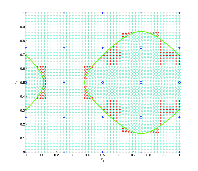 Error of testing data
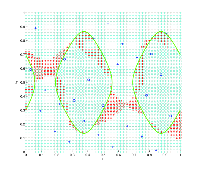 RKHS
RKHS
Error of testing data
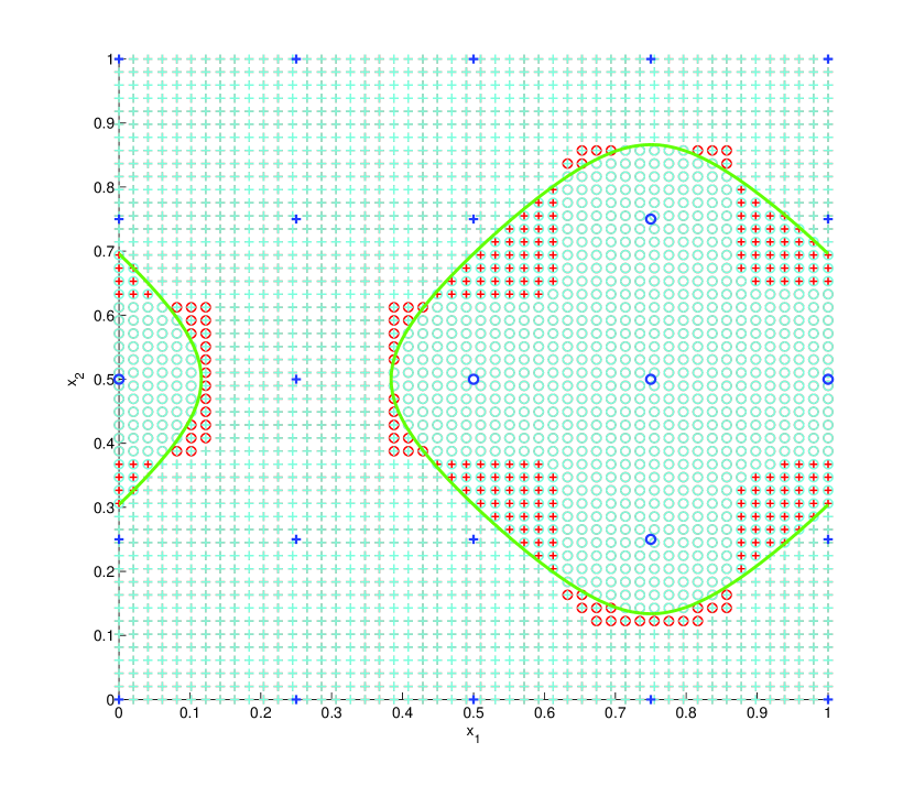 Error of testing data
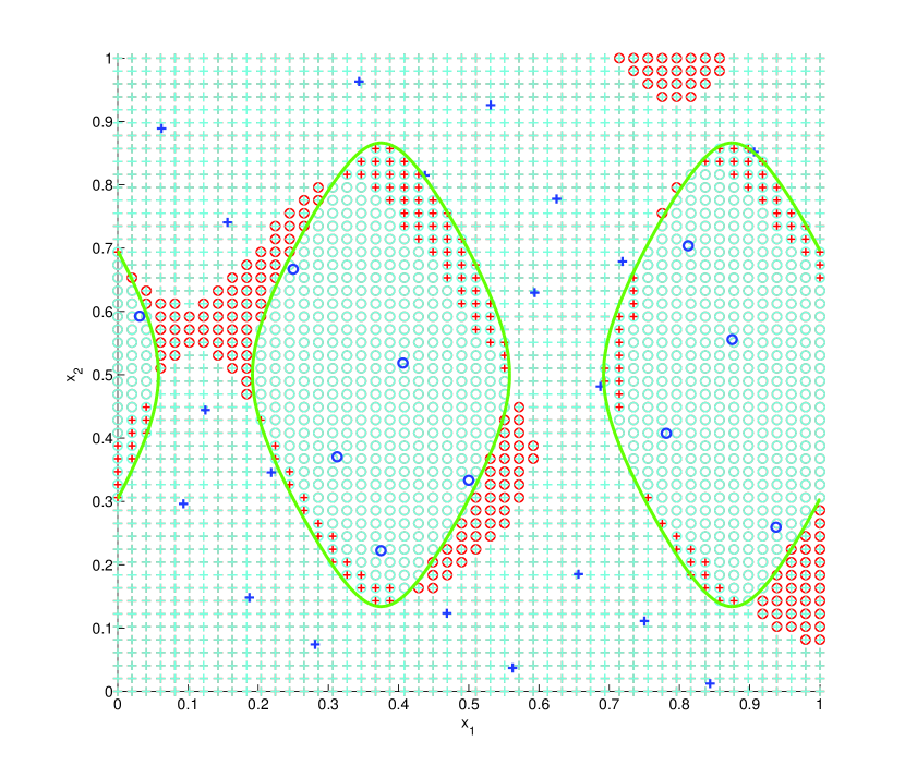 RKBS
RKBS
Remark 6.1.
In this article, we start from the generalized Mercer kernels to construct the -norm RKBSs such that the structures and the notations are consistent with the classical versions of RKHSs in books [Wah90, Wen05, Fas07, SC08]. For simplifying the complexities, the expansion sets of the generalized Mercer kernels are always fixed (see Remark 3.2). Actually, we also use the expansion sets to construct the -norm RKBSs and the reproducing kernels. Suppose that the linearly independent sets and satisfy conditions (C-) and (C-). Here and are thought as the left-sided and right-sided expansion sets, respectively. By Proposition 3.4, the generalized Mercer kernel is well-defined by the expansion sets and . Obviously, when we start from the expansion sets, then the generalized Mercer kernels and the -norm RKBSs are uniquely determined.
Acknowledgments
This research is supported in part by the United States National Science Foundation under grant DMS-1522332, by Guangdong Provincial Government of China through the “Computational Science Innovative Research Team” program and by the Natural Science Foundation of China under grants 11471013 and 91530117.
Yuesheng Xu
I would like to express my gratitude to the Philip T. Church postdoctoral fellowship of Syracuse University and the HKBU FRG grant of Hong Kong Baptist University for their supports of the research of machine learning in reproducing kernel Banach spaces. The current research of kernel-based methods for machine learning is supported by the grant of the “Thousand Talents Program” for junior scholars of China (C83024), by the grant of the Natural Science Foundation of China (11601162), and by the grant of South China Normal University (671082, S80835, and S81031).
Qi Ye (corresponding author)
Index
- is the collection of all positive integers,
- ,
- for ,
- ,
- is the collection of all integers,
- ,
- is the collections of all real numbers,
- is the -dimensional real space,
- is the collections of all complex numbers,
- is a circle,
- is a locally compact Hausdorff space equipped with a regular Borel measure ,
- is the support of the Borel measure ,
- is the normed space formed by the -dimensional space with the standard norm for ,
- is the collection of all countable sequences of scalars with the standard norm for ,
- is the subspace of with all countable sequence of scalars that converge to ,
- is the collection of all measurable functions defined on the domain ,
- is the standard -norm Lebesgue space defined on for ,
- ,
- is the collection of all continuous functions defined on the domain , when is compact then is endowed with uniform norm.
- is the collection of all regular signed Borel measures on endowed with their variation norms,
- is an inner-product space,
- is the inner product of ,
- is a normed space,
- is the dual space of ,
- is the norm of ,
- is the dual bilinear product defined on and ,
- denotes that two normed spaces and are isometrically isomorphic, that is, ,
- is the collection of all finite linear combinations of elements of a set of a linear vector space,
- is a kernel, for example, reproducing kernel, generalized Mercer kernel and positive definite kernel,
- is the adjoint kernel of , that is, ,
- is defined in equation (5.39),
- is the left-sided kernel set of the reproducing kernel ,
- is the right-sided kernel set of the reproducing kernel ,
- is the left-sided expansion set of the generalized Mercer kernel ,
- is the right-sided expansion set of the generalized Mercer kernel ,
- is the left-sided sequence set of the generalized Mercer kernel ,
- is the right-sided sequence set of the generalized Mercer kernel ,
- is the eigenvalues of the positive definite kernel ,
- is the eigenfunctions of the positive definite kernel ,
- is the -norm space induced by for ,
- is the -norm space induced by for ,
- is a loss function,
- is a regularization function,
- is ,
- is ,
- is a -risk,
- is a regularized empirical risk over RKBSs,
- is a regularized infinite-sample risk over RKBSs,
- is a regularized empirical risk over ,
- is the norm operator of , that is, for ,
- is the Gâteaux derivative,
- is the Fréchet derivative,
- is the standard Gâteaux derivative of the normed operator ,
- is the redefined Gâteaux derivative of the norm of , that is, when , and when ,
- is a point evaluation functional at , that is, ,
- is an left-sided integral operator of the kernel , that is, ,
- is an right-sided integral operator of the kernel , that is, ,
- is an adjoint operator of the integral operator for the space of continous functions, that is, ,
- is the identity map,
- is the map , that is, ,
- is the map , that is, ,
- is a left-sided upper-bound function of the generalized Mercer kernel , that is, or when ,
- is a right-sided upper-bound function of the generalized Mercer kernel , that is, or when ,
- is the map massing by the tensor product, that is, .
- is the map massing by the sum, that is,
- is the map massing by the tensor product, that is, .
- The linear independence of : if and only if , for any and any finite pairwise distinct elements ,
- Conditions (C-) of and : for all and all (Here and ),
- Conditions (C-) of and : for all and all ,
- Conditions (C-GEN) of and : for all and all ,
- Conditions (C-PDK) of and : for all ,
- Assumptions (A-) of : and are linearly independent and satisfy conditions (C-).
- Assumptions (A-) of : and are linear independent and satisfy conditions (C-).
- Assumptions (A-PDK) of : and satisfy conditions (C-PDK).
- Assumptions (A-ELR) of and : is convex and strictly increasing, and satisfies that is convex for any fixed and any fixed .
- Assumptions (A-GLR) of and : is convex, strictly increasing, and continuously differentiable, and satisfies that is convex for any fixed and any fixed , and the function driven by (see equation (2.29)) satisfies that is differentiable for any fixed and whenever .
References
- [AMP09] A. Argyriou, C.A. Micchelli, and M. Pontil, When is there a representer theorem? Vector versus matrix regularizers, J. Mach. Learn. Res. 10 (2009), 2507–2529.
- [AMP10] by same author, On spectral learning, J. Mach. Learn. Res. 11 (2010), 935–953.
- [Aro50] N. Aronszajn, Theory of reproducing kernels, Trans. Amer. Math. Soc. 68 (1950), 337–404.
- [BDE09] A.M. Bruckstein, D.L. Donoho, and M. Elad, From sparse solutions of systems of equations to sparse modeling of signals and images, SIAM Rev. 51 (2009), no. 1, 34–81.
- [BDF07] J.M. Bioucas-Dias and M.A.T. Figueiredo, A new twist: two-step iterative shrinkage/thresholding algorithms for image restoration, IEEE Trans. I 16 (2007), 2992–3004.
- [BGV92] B.E. Boser, I. Guyon, and V. Vapnik, A training algorithm for optimal margin classifiers, The Fifth Annual ACM Workshop on Computational Learning Theory (Pittsburgh, PA) (D. Haussler, ed.), ACM Press, 1992, pp. 144–152.
- [BR77] J. Bruck and E. Ronald, On the weak convergence of an ergodic iteration for the solution of variational inequalities for monotone operators in Hilbert space, J. Math. Anal. Appl. 61 (1977), no. 1, 159–164.
- [BT09] A. Beck and M. Teboulle, A fast iterative shrinkage-thresholding algorithm for linear inverse problems, SIAM J. Imaging Sci. 2 (2009), no. 1, 183–202.
- [BTA04] A. Berlinet and C. Thomas-Agnan, Reproducing Kernel Hilbert Spaces in Probability and Statistics, Kluwer Academic Publishers, Boston, MA, 2004.
- [Buh03] M.D. Buhmann, Radial Basis Functions: Theory and Implementations, Cambridge University Press, Cambridge, 2003.
- [CDVLL98] A. Chambolle, R.A. De-Vore, N.Y. Lee, and B.J. Lucier, Nonlinear wavelet image processing: variational problems, compression, and noise removal through wavelet shrinkage, IEEE Trans. Image Process. 7 (1998), 319–335.
- [CMX15] Z. Chen, C.A. Micchelli, and Y. Xu, Multiscale methods for Fredholm integral equations, Cambridge University Press, Cambridge, 2015.
- [CRT06] E.J. Candès, J.K. Romberg, and T. Tao, Stable signal recovery from incomplete and inaccurate measurements, Comm. Pure Appl. Math. 59 (2006), no. 8, 1207–1223.
- [CS02] F. Cucker and S. Smale, On the mathematical foundations of learning, Bull. Amer. Math. Soc. (N.S.) 39 (2002), no. 1, 1–49 (electronic).
- [CV95] C. Cortes and V. Vapnik, Support vector networks, Mach. Learn. 20 (1995), 273–297.
- [DDDM04] I. Daubechies, M. Defrise, and C. De-Mol, An iterative thresholding algorithm for linear inverse problems with a sparsity constraint, Comm. Pure Appl. Math. 57 (2004), no. 11, 1413–1457.
- [DE03] D.L. Donoho and M. Elad, Optimally sparse representation in general (nonorthogonal) dictionaries via minimization, Proc. Natl. Acad. Sci. USA 100 (2003), no. 5, 2197–2202 (electronic).
- [DLDMV00] L. De-Lathauwer, B. De-Moor, and J. Vandewalle, A multilinear singular value decomposition, SIAM J. Matrix Anal. Appl. 21 (2000), no. 4, 1253–1278 (electronic).
- [Duc77] J. Duchon, Splines minimizing rotation-invariant semi-norms in Sobolev spaces, Constructive Theory of Functions of Several Variables (Berlin) (W. Schempp and K. Zeller, eds.), Springer, 1977, pp. 85–100.
- [Duf01] D.G. Duffy, Green’s Functions with Applications, Chapman & Hall/CRC, Boca Raton, FL, 2001.
- [EF08] J.F. Erickson and G.E. Fasshauer, Generalized native spaces, Approximation theory XII: San Antonio 2007 (M. Neamtu and L.L. Schumaker, eds.), Mod. Methods Math., Nashboro Press, Brentwood, TN, 2008, pp. 133–142.
- [ET83] I. Ekeland and T. Turnbull, Infinite-dimensional optimization and convexity, University of Chicago Press, Chicago, IL, 1983.
- [Fas07] G.E. Fasshauer, Meshfree Approximation Methods with matlab, World Scientific Publishing Co. Pte. Ltd., Hackensack, NJ, 2007.
- [FHW12a] G.E. Fasshauer, F.J. Hickernell, and H. Woźniakowski, Average case approximation: convergence and tractability of Gaussian kernels, Monte Carlo and Quasi-Monte Carlo Methods 2010 (Warszawa) (L. Plaskota and H. Woźniakowski, eds.), Springer-Verlag, 2012, pp. 329–344.
- [FHW12b] by same author, On dimension-independent rates of convergence for function approximation with Gaussian kernels, SIAM J. Numer. Anal. 50 (2012), no. 1, 247–271.
- [FHY15] G.E. Fasshauer, F.J. Hickernell, and Q. Ye, Solving support vector machines in reproducing kernel Banach spaces with positive definite functions, Appl. Comput. Harmon. Anal. 38 (2015), 115–139.
- [FLF11] B. Fornberg, E. Larsson, and N. Flyer, Stable computations with Gaussian radial basis functions, SIAM J. Sci. Comput. 33 (2011), no. 2, 869–892.
- [FM12] G.E. Fasshauer and M.J. McCourt, Stable evaluation of Gaussian radial basis function interpolants, SIAM J. Sci. Comput. 34 (2012), no. 2, A737–A762.
- [FN03] M.A.T. Figueiredo and R.D. Nowak, An EM algorithm for wavelet-based image restoration, IEEE Trans. Image Process. 12 (2003), 906–916.
- [FY11] G.E. Fasshauer and Q. Ye, Reproducing kernels of generalized Sobolev spaces via a Green function approach with distributional operators, Numer. Math. 119 (2011), no. 3, 585–611.
- [FY13] by same author, Reproducing kernels of Sobolev spaces via a green kernel approach with differential operators and boundary operators, Adv. Comput. Math. 38 (2013), no. 4, 891–921.
- [Gau09] K.F. Gauss, Theory of Motion of the Heavenly Bodies Moving About the Sun in Conic Sections: A Translation of Theoria Motus, Hamburg: Friedrich Perthes and I.H. Besser, 1809.
- [Gil67] J.R. Giles, Classes of semi-inner-product spaces, Trans. Amer. Math. Soc. 129 (1967), 436–446.
- [GP13] A.G. García and A. Portal, Sampling in reproducing kernel Banach spaces, Mediterr. J. Math. 10 (2013), 1401–1417.
- [HTF09] T. Hastie, R. Tibshirani, and J. Friedman, The Elements of Statistical Learning, second ed., Springer-Verlag, New York, 2009.
- [Jam47] R.C. James, Orthogonality and linear functionals in normed linear spaces, Trans. Amer. Math. Soc. 61 (1947), 265–292.
- [Kar70] L.A. Karlovitz, Construction of nearest points in the , even, and norms, J. Approx. Theory 3 (1970), no. 2, 123–127.
- [KB09] T.G. Kolda and B.W. Bader, Tensor decompositions and applications, SIAM Rev. 51 (2009), no. 3, 455–500.
- [Kre89] R. Kress, Linear Integral Equations, Springer-Verlag, Berlin, 1989.
- [KW70] G.S. Kimeldorf and G. Wahba, A correspondence between Bayesian estimation on stochastic processes and smoothing by splines, Ann. Math. Statist. 41 (1970), 495–502.
- [LMSX12] Q. Li, C.A. Micchelli, L. Shen, and Y. Xu, A proximity algorithm accelerated by Gauss-Seidel iterations for L1/TV denoising models, Inverse Problems 28 (2012), no. 9, 095003, 20.
- [LSXZ15] Q. Li, L. Shen, Y. Xu, and N. Zhang, Multi-step fixed-point proximity algorithms for solving a class of optimization problems arising from image processing, Adv. Comput. Math. 41 (2015), no. 2, 387–422.
- [Lum61] G. Lumer, Semi-inner-product spaces, Trans. Amer. Math. Soc. 100 (1961), 29–43.
- [Meg98] R.E. Megginson, An Introduction to Banach Space Theory, Springer-Verlag, New York, 1998.
- [Mes62] H. Meschkowski, Hilbertsche Räume mit Kernfunktionen, Springer-Verlag, Berlin, 1962.
- [MP04] C.A. Micchelli and M. Pontil, A function representation for learning in Banach spaces, Learning theory (J. Shawe-Taylor and Y. Singer, eds.), Springer-Verlag, Berlin, 2004, pp. 255–269.
- [MSX11] C.A. Micchelli, L. Shen, and Y. Xu, Proximity algorithms for image models: denoising, Inverse Problems 27 (2011), no. 4, 045009, 30.
- [MSXZ13] C.A. Micchelli, L. Shen, Y. Xu, and X. Zeng, Proximity algorithms for the L1/TV image denoising model, Adv. Comput. Math. 38 (2013), no. 2, 401–426.
- [MXZ06] C.A. Micchelli, Y. Xu, and H. Zhang, Universal kernels, J. Mach. Learn. Res. 7 (2006), 2651–2667.
- [Pas79] G.B. Passty, Ergodic convergence to a zero of the sum of monotone operators in Hilbert space, J. Math. Anal. Appl. 72 (1979), no. 2, 383–390.
- [PB14] N. Parikh and S. Boyd, Proximal algorithms, Found. Trends Optim. 1 (2014), no. 3, 127–239.
- [REC+03] B.D. Rao, K. Engan, S.F. Cotter, J. Palmer, and K. Kreutz-Delgado, Subset selection in noise based on diversity measure minimization, IEEE Trans. Signal Process. 51 (2003), 760–770.
- [Rie07] F. Riesz, Sur une espèce de géométrie analytique des systèmes de fonctions sommables, C. R. Acad. Sci. Paris 144 (1907), 1409–1411.
- [Rie09] by same author, Sur les opérations fonctionnelles linéaires, C. R. Acad. Sci. Paris 149 (1909), 974–977.
- [RKD99] B.D. Rao and K. Kreutz-Delgado, An affine scaling methodology for best basis selection, IEEE Trans. Signal Process. 47 (1999), 187–200.
- [Rud87] W. Rudin, Real and Complex Analysis, third ed., McGraw-Hill Book Co., New York, 1987.
- [SC08] I. Steinwart and A. Christmann, Support Vector Machines, Springer-Verlag, New York, 2008.
- [SFL11] B.K. Sriperumbudur, K. Fukumizu, and G.R.G. Lanckriet, Learning in Hilbert vs.Banach spaces: a measure embedding viewpoint., Advances in Neural Information Processing Systems (Cambridge) (J. Shawe-Taylor, R.S. Zemel, P.L. Bartlett, F. Pereira, and K.Q. Weinberger, eds.), MIT Press, 2011, pp. 1773–1781.
- [SHS01] B. Schölkopf, R. Herbrich, and A.J. Smola, A generalized representer theorem, Computational learning theory (Amsterdam) (D. Helmbold and B. Williamson, eds.), Springer-Verlag, Berlin, 2001, pp. 416–426.
- [SS02] B. Schölkopf and A.J. Smola, Learning with Kernels, MIT Press, Cambridge, Massachusetts, 2002.
- [Ste03] I. Steinwart, Sparseness of support vector machines, J. Mach. Learn. Res. 4 (2003), 1071–1105.
- [SW06] R. Schaback and H. Wendland, Kernel techniques: from machine learning to meshless methods, Acta Numer. 15 (2006), 543–639.
- [SX10] G. Song and Y. Xu, Approximation of high-dimensional kernel matrices by multilevel circulant matrices, J. Complexity 26 (2010), no. 4, 375–405.
- [SZ04] S. Smale and D.-X. Zhou, Shannon sampling and function reconstruction from point values, Bull. Amer. Math. Soc. (N.S.) 41 (2004), no. 3, 279–305 (electronic).
- [SZ11] G. Song and H. Zhang, Reproducing kernel Banach spaces with the norm II: Error analysis for regularized least square regression, Neural Comput. 23 (2011), no. 10, 2713–2729.
- [SZH13] G. Song, H. Zhang, and F.J. Hickernell, Reproducing kernel Banach spaces with the norm, Appl. Comput. Harmon. Anal. 34 (2013), no. 1, 96–116.
- [VHK13] T. Villmann, S. Haase, and M. Kästner, Gradient based learning in vector quantization using differentiable kernels, Advances in Self-Organizing Maps (Santiago, Chile) (P.A. Estévez, J.C. Príncipe, and P. Zegers, eds.), Springer-Verlag, 2013, pp. 193–204.
- [VL63] V.N. Vapnik and A. Lerner, Pattern recognition using generalized portrait method, Auto. Rmote Control 24 (1963), 774–780.
- [Wah90] G. Wahba, Spline Models for Observational Data, Society for Industrial and Applied Mathematics (SIAM), Philadelphia, PA, 1990.
- [Wen05] H. Wendland, Scattered Data Approximation, Cambridge University Press, Cambridge, 2005.
- [Ye12] Q. Ye, Analyzing reproducing kernel approximation method via a Green function approach, Ph.D. thesis, Illinois Institute of Technology, Chicago, 2012.
- [Ye14] Q. Ye, Support vector machines in reproducing kernel Hilbert spaces versus Banach spaces, Approximation Theory XIV: San Antonio 2013 (New York) (G.E. Fasshauer and L.L. Schumaker, eds.), Springer-Verlag, 2014, pp. 377–395.
- [Zho03] D.-X. Zhou, Capacity of reproducing kernel spaces in learning theory, IEEE Trans. Inform. Theory 49 (2003), no. 7, 1743–1752.
- [Zwi09] B. Zwicknagl, Power series kernels, Constr. Approx. 29 (2009), no. 1, 61–84.
- [ZXZ09] H. Zhang, Y. Xu, and J. Zhang, Reproducing kernel Banach spaces for machine learning, J. Mach. Learn. Res. 10 (2009), 2741–2775.
- [ZZ12] H. Zhang and J. Zhang, Regularized learning in Banach spaces as an optimization problem: representer theorems, J. Global Optim. 54 (2012), no. 2, 235–250.