Intermittent dislocation density fluctuations in crystal plasticity from a phase-field crystal model

Abstract

Plastic deformation mediated by collective dislocation dynamics is investigated in the two-dimensional phase-field crystal model of sheared single crystals. We find that intermittent fluctuations in the dislocation population number accompany bursts in the plastic strain-rate fluctuations. Dislocation number fluctuations exhibit a power-law spectral density $1/f^{2}$ at high frequencies $f$. The probability distribution of number fluctuations becomes bimodal at low driving rates corresponding to a scenario where low density of defects alternate at irregular times with high population of defects. We propose a simple stochastic model of dislocation reaction kinetics that is able to capture these statistical properties of the dislocation density fluctuations as a function of shear rate.

Small-scale plasticity is characterized by intermittent strain-rate fluctuations and strain avalanches that follow robust power-law statistics, with detailed reports for both crystalline materials  Richeton et al. (2005, 2006); Greer et al. (2009) and amorphous materials Argon (2013). Discrete dislocation dynamics simulations have been successful in reproducing the power-law statistics of strain avalanches in crystal plasticity assuming that the microscopic origin of intermittency is attributed to dissipative processes associated with crystal defects, such as dislocations and disclinations Miguel et al. (2001); Ispánovity et al. (2010); Tsekenis et al. (2013). The scaling behavior observed near plastic yielding was initially explained by analogy to the depinning phase transition Friedman et al. (2012); Tsekenis et al. (2013); LeBlanc et al. (2012). However, recent numerical simulations and experiments show that a scale free behavior of plastic bursts occurs also at applied stresses away from the yielding point, which makes the relation to nonequilibrium depinning transition a controversional topic Ispánovity et al. (2014, 2013).

As the global plastic strain rate, $\dot{\gamma}$, is directly proportional to the mobile dislocation density $\rho_{d}$ and mean velocity $\langle v\rangle$ by Orowan’s relation: $\dot{\gamma}\approx b\rho_{d}\langle v\rangle$, the intermittency of $\dot{\gamma}$ is influenced both by the collective dislocation velocity (typically following stick-slip dynamics) and dislocation number fluctuations. Previous work on plastic avalanches has only taken into account the stick-slip motion of crystal defects, due to the challenging nature of modeling dislocation density fluctuations naturally, without introducing artifacts due to ad hoc rules for dislocation reactions. The question that concerns us here is: what is the effect of dislocation number fluctuations, particularly near the yielding transition?

The purpose of this Letter is to investigate numerically the density fluctuations of mobile dislocations as a crystal is sheared near and away from yielding point. Conventional techniques that solve the equations of motion for discrete dislocations are not appropriate, because they would require ad hoc rules for dislocation annihilation and creation. Instead, we use the phase-field crystal approach Elder and Grant (2004) which has been shown to be an efficient technique to model plastic deformations in single and poly-crystals, one which can capture implicitly dislocation dynamics and interactions Emmerich et al. (2012); Berry et al. (2014). Working in two dimensions, we find that the total number of defects $N_{d}$ is a highly fluctuating quantity whose power spectrum at large frequency $f$ is characterized by a $1/f^{2}$ scaling, similar to that of the global plastic strain rate. Also, $N_{d}$ follows a non-trivial probability distribution which becomes bimodal at small driving rates, reflecting that both dislocation extinction events and a dense population of interacting dislocations occur with a non-zero probability. Finally, we develop a stochastic coarse-grained model for the effective continuum mechanics of our phase-field crystal model, based upon previous work that has successfully described the regime of cyclic loading and plastic regime where dislocations self-organize into cell-like patterns Hähner (1996a, b); Ananthakrishna (2007). In this way, we are able to calculate the power spectrum of dislocation number fluctuations, obtaining results in agreement with our simulations. While we have not performed extensive tests in three dimensional systems, our stochastic model seems to remain valid despite the more complex defect structures admissible in three dimensions.

Sheared phase-field crystal:- We use the phase-field crystal (PFC) model to study intermittent plastic deformation in single crystals. The PFC model describes the evolution of an order parameter field $\psi(\bm{r},t)$ that is related to the particle number density averaged over atomic vibration timescales, i.e. $\psi\sim\langle\sum_{i}\delta(\bm{r}-\bm{r}_{i})\rangle_{t}$. An effective Swift-Hohenberg free-energy functional is formulated in the lowest order gradient expansion of $\psi$-field and given as Elder and Grant (2004) $\mathcal{F}\{\psi\}=\int d\bm{r}\left[\frac{1}{2}\psi\left(q_{0}^{2}+\nabla^{2}\right)^{2}\psi+\frac{r}{2}\psi^{2}+\frac{1}{4}\psi^{4}\right]$, where $r\sim(T-T_{c})/T_{c}<0$ is the quenching depth parameter related to the deviation from the critical melting temperature, and $q_{0}=2\pi/a$ with $a$ being the equilibrium lattice spacing. The equilibrium phase diagram obtained from the free energy $\mathcal{F}\{\psi\}$ contains a region in the $(r,\psi_{0})$-space where the system relaxes to a spatially periodic $\psi$-field around a mean crystal density $\psi_{0}$, that corresponds to a crystalline phase with triangular symmetry in two-dimensions Elder and Grant (2004).

The dynamics of the $\psi$-field that includes both the diffusive timescale of phase transformation and elastic strain relaxation is given by a damped wave equation Stefanovic et al. (2006)

$$\frac{\partial^{2}\psi}{\partial t^{2}}+\beta\frac{\partial\psi}{\partial t}=-\nabla\cdot\bm{J},$$ (1)

where the density current has a diffusive part determined by the free energy $\mathcal{F}$ and an advective part that simulates the strain rate boundary conditions, namely $\bm{J}=-\alpha^{2}\nabla\frac{\delta\mathcal{F}}{\delta\psi}+\beta\bm{v}\psi$, where $\alpha^{2}$ is the diffusivity coefficient and $\beta$ is the overdamped coefficient. Physically, these two parameters are related to the effective sound speed and vacancy diffusion coefficient that set a finite elastic interaction length $L^{*}$ and time $t^{*}$ Stefanovic et al. (2009). Their values are constrained by the thermodynamic stability of the crystalline phase and the damping rate of the elastic excitations. From a linear stability analysis around the one-mode approximation solution of $\psi$, the dispersion relation corresponding to Eq. (1) with $\bm{v}=0$ describes a pair of density waves that propagate undamped for a time $t^{*}\approx 2\beta^{-1}$ over a lengthscale $L^{*}\approx v_{eff}t^{*}$, with an effective wave speed $v_{eff}\approx 2\alpha\sqrt{3\psi_{0}^{2}+r+q_{0}^{4}+9A_{0}^{2}/8}$, where $A_{0}=4/5(\psi_{0}+1/3\sqrt{-15r-36\psi_{0}^{2}})$ is the amplitude of $\psi$ in the one-mode approximation Stefanovic et al. (2009). For timescales $t>t^{*}$, the density disturbance propagates diffusively with a vacancy diffusion coefficient $D_{0}=\alpha^{2}(3\rho^{2}+r+q_{0}^{4}+9A_{0}^{2}/8)/\beta$. The model parameters are chosen such that the timescale $t^{*}$ of strain wave relaxation is much smaller than the diffusion one. We impose a constant strain rate boundary condition similar to that used in Ref. Chan et al. (2010). The velocity field $\bm{v}=(v_{x}(y),0)$ acts effectively only on a small strip on the top and bottom boundaries,

$$v_{x}(y)=v_{0}e^{-\frac{L-y}{\lambda}}H\left(y-\frac{L}{2}\right)-v_{0}e^{-\frac{y}{\lambda}}H\left(\frac{L}{2}-y\right),$$ (2)

where $H(x)$ is the Heaviside step function and the penetration length $\lambda$ of the imposed shear velocity is chosen to be much smaller than the system size $L$.

We solve Eq. (1) numerically on a two-dimensional rectangular $L\times L$ domain of size $512dx\times 512dx$, using both a finite difference method with an isotropic discretization of the gradients and the Laplace operator Angheluta et al. (2012) as well as a spectral method utilizing discrete cosine transforms similar to that in Ref. Tegze et al. (2009). In the spectral method implementation, we added a conservative, Gaussian noise term to Eq. (1) to enable dislocation nucleation in the regime of low dislocation density. Regardless of the noise term or numerical implementation, we observe robust statistical properties. The discretization parameters are set to $dt=0.015$, $dx=1$, and $a=2\pi$. The boundary conditions are periodic in the $x$- direction and with zero-flux in the $y$-direction at $0$ and $L$. As initial condition, we use the relaxed equilibrium solution of a single crystal at a fixed undercooling depth $r=-0.5$ and $\psi_{0}=0.3$. The damping coefficient is set to $\beta=0.5$ and the diffusivity parameter $\alpha=15$. These parameter values give a typical wave speed of $v_{eff}\approx 36$, an elastic interaction length $L^{*}\approx 146$, and a characteristic damping time $t^{*}\approx 4$. We set $\lambda=0.05L<L^{*}$, thus the strain waves propagate deeper into the bulk of the crystal before they are dissipated. However, in a constant strain-rate experiment, the imposed shear rate should be sufficiently slow such that the elastic waves decay almost ‘instantaneously’. Under these conditions, we vary the imposed shear velocity between $v_{0}\approx 4.3-8.4$, that corresponds to an applied strain rate varying between $\dot{\epsilon}_{0}=\lambda v_{0}/(2L^{2})\approx 2.10-4.10\times 10^{-4}$ in arbitrary time units.

(a)               (b)

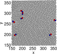
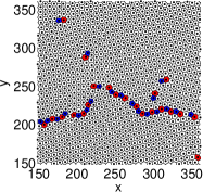
(c)               (d)

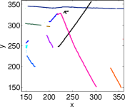
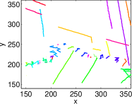
Figure 1: (Color online) Different dislocation configurations in the Voronoi diagram (panels (a) and (b)) corresponding to a crystal that is sheared at constant rate $\dot{\epsilon}_{0}=3\times 10^{-4}s^{-1}$. Dislocations are represented as pairs of 5-fold and 7-fold defect atoms shown in red and blue. The trajectories of these dislocations are depicted (random coloring) in the bottom panels, (c) for a dilute configuration of dislocations and (d) for a more dense distribution of dislocations organized into a wall sweeping across the system.

Dislocation density fluctuations:- Plastic deformations induce vacancies and point topological defects that are represented by phase and amplitude modulations in the $\psi$-field. These defects are harder to locate and track accurately from the crystal density field. Instead, we use a more atomistic approach of tracking the atoms neighboring different point defects. For a perfect fcc lattice in two dimensions, each PFC atom (located as a minimum in the $\psi$-field) is surrounded by $6$ nearest neighbors, but near a point defect the coordination number is different. Defect atoms with coordination number $5$ or $7$ are associated with disclinations, and typically pair up to form a dislocation as illustrated in Figure (1).

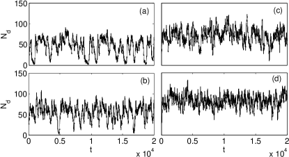
Figure 2: (Color online) Temporal fluctuations in the dislocation number for different strain rates. From (a) to (d) the strain rate increases as $2.78\times 10^{-4}$, $3.02\times 10^{-4}$, $3.41\times 10^{4}$, and $3.90\times 10^{-4}$.

We focus on the interaction and dynamics of dislocations which are defined as pairs of $5$ and $7$-fold defect atoms. The number of dislocations varies with the system size and the applied strain rate, and, for our parameter values, it is up to $\mathcal{O}(10^{2})$. For a given strain rate, the dislocation density is both highly heterogeneous in space and intermittent in time. The spatial density of dislocations varies from dilute configuration of single, fast-moving dislocations to denser configurations of dislocation pile-ups that slowly sweep across the sheared crystal (see Figure (1) (a)-(b)). The trajectories of isolated dislocations follow the slip planes at fast speeds, in contrast to the slow motion of correlated dislocations (see Figure (1) (c)-(d)). The alternations between configurations of fast and slow moving dislocations result in sporadic fluctuations of the plastic strain rate that is related to the global dislocation velocity. Ref. Chan et al. (2010) studied the avalanche statistics of the global strain rate signal showing that the power-law exponent of the energy dissipated during avalanches is in agreement with that predicted near a depinning transition in the mean field approximation. Here we study instead the nontrivial statistical properties of the dislocation density fluctuations. A detail analysis of the relation between the statistics of number fluctuations and a depinning phase transition is the subject of a separate study.

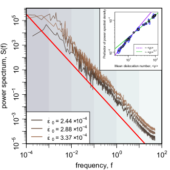
Figure 3: (Color online) Power spectrum of the dislocation number fluctuations $N_{d}$ vs. frequency $f$ for different strain rates. The red line shows the prediction of the stochastic model Eq. (4), varying as $C/f^{2}$ for large $f$. The inset shows the dependence of $C$ on the mean dislocation number. The error bars in the inset are given along the principal axes of the variation over multiple simulations of the mean of $N_{d}$ and $C$.

We observe that sudden dislocation reactions (annihilations or creations) occur at irregular times between isolated dislocations or between an isolated dislocation and a domain wall. The latter event may lead to the breaking-up of the domain wall and the release of fast-moving dislocations along different gliding planes. The total dislocation number $N_{d}$ is a highly fluctuating quantity depending on the imposed shear rate, such that, at low strain rates, it is characterized by temporal variations around a mean set by the external driving interspersed with short episodes of almost dislocation extinction, as seen in Figure (2). For $\dot{\epsilon}_{0}<2.00\times 10^{-4}$, keeping the same values for the other parameters, we observe that the vanishing dislocation density becomes an absorbing state after an initial transient time of fluctuations. In this dynamical regime, the crystal has been rotated such that the stored energy is mainly dissipated by visco-elastic deformation without the nucleation of defects.

In Figure (3), we show the power spectrum $S(f)=\langle|\hat{N}_{d}|^{2}\rangle$, where $\hat{N}_{d}$ is the Fourier transform of $N_{d}$, computed from the time signals illustrated in Figure (2). The power spectrum has a power-law decay at high frequencies $f$ given by $C/f^{2}$. To test that this scaling behavior arises of the density fluctuations from correlated events, we have measured the dependence of the scaling coefficient $C$ on $\langle N_{d}\rangle$ shown in the inset of Figure (3). For low shear rates corresponding a dilute dislocation density, the coefficient exhibits a linear scaling, that is consistent with uncorrelated, random dislocation reactions. At higher shear rates, the dependence changes to a power-law implying that the signal arises from correlated dislocation dynamics.

For each constant shear rate $\dot{\epsilon}_{0}$, we also measure the probability distribution function (PDF) of the distribution number as shown in Figure (4). At low $\dot{\epsilon}_{0}$’s, the PDF $P(N_{d})$ is bimodal with one peak near zero corresponding to the frequency of dislocation extinctions and the other peak centered around a mean value imposed by the external shear rate. At higher values of $\dot{\epsilon}_{0}$, the probability that the dislocation number drops to zero becomes vanishingly small, and approaches a uni-modal form with the peak shifting to the right as the driving force is increased.

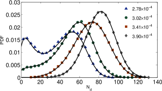
Figure 4: (Color online) Probability distribution function of dislocation density fluctuations corresponding to PFC single crystals sheared at different shear rates. The continuous lines represent the stationary probability distributions predicted by the stochastic model of dislocation number fluctuations from Eq. (14). Numerical values of the model fitting parameters are tabulated below.

$\dot{\epsilon}_{0}$	$2.78\times 10^{-4}$	$3.02\times 10^{-4}$	$3.41\times 10^{4}$	$3.90\times 10^{-4}$
$k$	$0.31$	$0.62$	$2.67$	$3.20$
$D$	$0.09$	$0.09$	$0.18$	$0.12$
$m$	$26.01$	$28.08$	$29.08$	$31.15$

Stochastic model:- The $1/f^{2}$ signal signature leads us to adopt a stochastic approach for the description of the dynamics of mobile dislocations initially proposed by Hähner Hähner (1996a, b) to describe dislocation cell formation and fractal patterning during various plastic deformation regimes. The basic idea is that the intrinsic stress and strain-rate fluctuations, arising from long-range interactions between dislocations, may lead to noise-induced non-equilibrium phase transitions corresponding to different plastic deformation regimes and dislocation patterning. The microscopic details of dislocation interactions are neglected and effectively replaced by a stochastic contribution to the mean field. Thus, one can write a general evolution equation of the dislocation density $\rho_{d}=N_{d}/\mathcal{V}$, where $\mathcal{V}$ is the crystal volume in which dislocations are embedded, as

$$\dot{\rho}_{d}=R(\rho_{d},\dot{\epsilon}),$$ (3)

where dislocation reactions depend on the strain-rate $\dot{\epsilon}$ and the defect density $\rho_{d}$. We decompose the strain-rate into a deterministic part related to the external driving and a stochastic part related to dislocation interactions, $\dot{\epsilon}=\langle\dot{\epsilon}\rangle+\delta\dot{\epsilon}$. The simplest assumption is that all reactions rate depend linearly on the stochastic strain rate, so that Eq. (3) reduces to a Langevin equation of the form

$$\dot{\rho}_{d}=F(\rho_{d},\langle\dot{\epsilon}\rangle)+G(\rho_{d})\delta\dot{\epsilon},$$ (4)

where $F(\rho_{d},\langle\dot{\epsilon}\rangle)$ describes the deterministic reaction rates depending on the current dislocation density and the mean strain rate, while $G(\rho_{d})$ models the stochastic reaction rate due to mutual dislocation interactions depending on the density $\rho_{d}$. The strain-rate fluctuations $\delta\dot{\epsilon}(t)$ are approximated by a Gaussian white noise with zero mean and covariance $\langle\delta\dot{\epsilon}(t)\delta\dot{\epsilon}(t^{\prime})\rangle=2D\delta(t-t^{\prime})$, while the noise amplitude $\sqrt{D}$ measures the effective contribution of dislocation interactions. The white noise-limit is taken under the approximation that the strain-rate fluctuations are typically short-ranged compared to the timescale of dislocation evolution and patterning Hähner (1996a). The probability distribution function of dislocation density $P(\rho_{d})$ follows from Eq. (4) as the steady state solution of the Fokker-Planck equation in the Stratonovich formulation with natural boundary conditions and given as

$$P(\rho_{d})=\frac{\mathcal{N}}{G(\rho_{d})}\exp\left(\int_{0}^{\rho_{d}}dx\frac{F(\rho)}{DG^{2}(\rho)}\right),$$ (5)

where $\mathcal{N}^{-1}=\int_{0}^{\infty}d\rho_{d}G^{-1}(\rho_{d})\exp\left(\int_{0}^{\rho_{d}}d\rho f(\rho)D^{-1}G^{-2}(\rho)\right)$ is the normalization constant. We assume that the deterministic part of the dislocation reactions is driven by a potential field, i.e. $F(\rho_{d})=-U^{\prime}(\rho_{d})$, that is approximated to the lowest order by a double-well potential $U(\rho_{d})=\frac{1}{4}\left(\frac{\rho_{d}}{m}-1\right)^{4}-\frac{1}{2}\left(\frac{\rho_{d}}{m}-1\right)^{2}-\kappa\left(\frac{\rho_{d}}{m}-1\right)$, with the two minima corresponding to zero density and a mean density related to the mean strain rate. Thus, the scaling parameter $m$ locates the mean density that increases monotonically with the shear rate $\dot{\epsilon}_{0}$ (also seen from the table in Figure (4)). $\kappa$ is a parameter that also increases with $\dot{\epsilon}_{0}$ and favors a finite mean density. As $\kappa\rightarrow 0$, dislocation extinction events and a finite population of interacting dislocations both occur with non-zero probabilities. The noise intensity in Eq. (4) depends on the dislocation density, such that it is able to simulate the internal interactions between dislocations. To this end, we assume a linear relationship given by $G(\rho_{d})=1+\rho_{d}/m$. With these specific expressions of the reaction rates, we find that the PDF of $\rho_{d}$ given generically by Eq. (13) becomes equal to

$$P(\rho_{d})=\mathcal{N}\left(1+\frac{\rho_{d}}{m}\right)^{-1-11/D}\exp\left(-\frac{\mathcal{L}(\rho_{d})}{2D}\right),$$ (6)

where $\mathcal{L}=\frac{\rho_{d}}{m^{2}(m+\rho_{d})}(\rho_{d}^{2}-9m\rho_{d}-2m^{2}\kappa-22m^{2})$. The stationary distribution of this simple stochastic model of dislocation reactions captures very well the empirical PDF obtained from the phase-field crystal simulations as seen in Figure (4). We have also verified numerically that our stochastic model is able to reproduce the $1/f^{2}$ spectral density of number fluctuations. An analytical calculation of the high-frequency limit of the power-spectrum using the results of Refs. Caroli et al. (1982); Brey et al. (1984); Sigeti and Horsthemke (1987) is given in the Supplemental Material. There we show that the correlation function $C(t)=\langle\rho_{d}(0)\rho_{d}(t)\rangle$ can be calculated in general as a power series of the form $C(t)=\sum_{n=0}^{\infty}\frac{(-t)^{n}}{n!}\langle x(\mathcal{O}^{\dagger})^{n}x\rangle$, where $\mathcal{O}^{\dagger}=-\left[F+DG^{\prime}G)\right]\frac{\partial}{\partial\rho_{d}}-DG^{2}\frac{\partial^{2}}{\partial\rho_{d}^{2}}$ is the adjoint Kolmogorov operator corresponding to Eq. (4). Hence, the large $f$ limit of the power spectrum $S(f)=2\Re\{\int_{0}^{\infty}dte^{-2\pi ift}C(t)\}$ is dominated by the first non-zero term in the expansion and given as $S(f)\approx\langle\rho_{d}\mathcal{O}^{\dagger}\rho_{d}\rangle f^{-2}$, where $\langle\rho_{d}\mathcal{O}^{\dagger}\rho_{d}\rangle=-\langle\rho_{d}[F+DG^{\prime}G]\rangle$ is determined by the first four moments of the steady state $P(\rho_{d})$. Thus, the high frequency power spectrum is proportional to $1/f^{2}$, with the proportionality constant depending on the mean density and higher moments, a result that is expected to be robust in higher dimensions and testable in experiment.

In conclusion, by using the phase field crystal model, we showed that number fluctuations of dislocations follow non-Gaussian statistics with a $1/f^{2}$ power spectrum similar to that of strain rate fluctuations. This behavior arises from correlated dislocation reactions, and can be accurately captured by a stochastic model which makes experimentally testable predictions for the probability distribution of defect numbers as a function of shear rate.

Supplementary Information

The dislocation density fluctuations are modelled by a non-linear Langevin equation with multiplicative noise given generically as

$$\dot{x}=f(x)+g(x)\xi(t),$$ (7)

where the noise term is related to the strain-rate fluctuations due to dislocation interactions, and $\xi(t)$ is approximated by a Gaussian white noise with zero mean

$$\langle\xi(t)\xi(t^{\prime})\rangle=2D\delta(t-t^{\prime}),$$ (8)

with the $D$ a parameter of noise amplitude that measures the effective contribution of dislocation interactions. The deterministic part $f(x)$ describes the dislocation reaction rate and it is driven by a potential field, i.e. $f(x)=-dU(x)/dx$, that is approximated to the lowest order by a double-well potential

$$U(x)=\frac{1}{4}\left(\frac{x}{m}-1\right)^{4}-\frac{1}{2}\left(\frac{x}{m}-1\right)^{2}-\kappa\left(\frac{x}{m}-1\right),$$ (9)

with the two minima corresponding to zero density and a mean density related to the mean strain rate. Thus, the scaling parameter $m$ locates the mean density that increases monotonically with the shear rate $\dot{\epsilon}_{0}$. $\kappa$ is a parameter that also increases with $\dot{\epsilon}_{0}$ and favours a finite mean density. As $\kappa\rightarrow 0$, dislocation extinction events and a finite population of interacting dislocations both occur with non-zero probabilities. The noise intensity in Eq. (7) depends on the dislocation density, such that it is able to simulate the internal interactions between dislocations. To this end, we assume a linear relationship given by $g(x)=1+x/m$.

For a generic Langevin equation with additive noise, there is a general argument to determine the high-frequency limit of the noise power-spectrum Caroli et al. (1982); Brey et al. (1984); Sigeti and Horsthemke (1987). One can show that the power spectrum density $S(\omega)$ of one-dimensional stochastic fluctuations decays asymptotically as $1/\omega^{2}$ for additive Gaussian noise regardless of expression of the deterministic drive Caroli et al. (1982); Brey et al. (1984), whereas for a second-order, additive Langevin equation, $S(\omega)$ is dominated by $1/\omega^{4}$ as $\omega\rightarrow\infty$. Here, we present a general derivation of $S(\omega)$ in the high-$\omega$ limit for a fist-order, multiplicative Langevin equation given by Eq. (7).

The multiplicative noise in Eq. (7) is studied using the Stratonovich calculus when the strain-rate fluctuations are considered in the $\delta$-correlated limit. Henceforth, the corresponding Fokker-Planck equation is given by

$$\frac{\partial P(x,t)}{\partial t}=-\mathcal{O}P(x,t),$$ (10)

where $P(x,t)$ is the probability distribution function and the propagation operator $\mathcal{O}$ in the Stratonovich definition takes the form

$$\mathcal{O}=\frac{\partial}{\partial x}\left[f(x)+Dg^{\prime}(x)g(x)\right]-D\frac{\partial^{2}}{\partial x^{2}}g^{2}(x).$$ (11)

Similar results are also obtained in the Ito calculus for which the $g$-dependent term in the drift term is removed.

The formal solution of Eq. (10) with the initial condition $P(x_{0},0)=\delta(x-x_{0})$ can be expressed as

$$P(x,t|x_{0},0)=e^{-\mathcal{O}t}\delta(x-x_{0}).$$ (12)

Also the stationary probability distribution $P_{st}(x)$ of Eq. (10) is

$$P_{st}(x)=\frac{\mathcal{N}}{g(x)}\exp\left(\int_{0}^{x}dy\frac{f(y)}{Dg^{2}(y)}\right),$$ (13)

where $\mathcal{N}^{-1}=\int_{0}^{\infty}dxg^{-1}(x)\exp\left(\int_{0}^{x}dyf(y)D^{-1}g^{-2}(y)\right)$ is the normalization constant. With the specific expressions of the reaction rates that we considered for our model, we find that the PDF of $x$ given generically by Eq. (13) becomes equal to

$$P_{st}(x)=\mathcal{N}\left(1+\frac{x}{m}\right)^{-1-11/D}\exp\left(-\frac{\mathcal{L}(x)}{2D}\right),$$ (14)

where $\mathcal{L}=\frac{x}{m^{2}(m+x)}(x^{2}-9mx-2m^{2}\kappa-22m^{2})$.

The power spectrum density $S(\omega)$ is defined as the Fourier transform of the time correlation function and given as

$$S(\omega)=\frac{1}{\pi}Re\int_{0}^{\infty}d\omega e^{-i\omega t}C(t),$$ (15)

where the time correlation function is

$$C(t) = \langle x(t)x(0)\rangle$$ (16)

$$= \int dx\int dx_{0}xP(x,t|x_{0},0)x_{0}P_{st}(x_{0}).$$

Using the formal solution of the transition probability from Eq. (12), we can integrate over $x_{0}$ and arrive at

$$C(t) = \int dxxe^{-\mathcal{O}t}xP_{st}(x)$$ (17)

$$= \int dxP_{st}(x)\left(xe^{-\mathcal{O}^{\dagger}t}x\right)=\langle xe^{-\mathcal{O}^{\dagger}t}x\rangle,$$

where $\langle\cdot\rangle$ represents an average with respect to the stationary distribution $P_{st}$. The adjoint operator $\mathcal{O}^{\dagger}$ is defined from the relation $\int dx\psi(x)\mathcal{O}\phi(x)=\int dx\phi(x)\mathcal{O}^{\dagger}\psi(x)$ and after integration by parts is given as

$$\mathcal{O}^{\dagger}=-\left[f(x)+Dg^{\prime}(x)g(x)\right]\frac{\partial}{\partial x}-Dg^{2}(x)\frac{\partial^{2}}{\partial x^{2}}.$$ (18)

Expanding the exponential in Eq. (17), we have that

$$C(t) = \sum_{n=0}^{\infty}\frac{(-t)^{n}}{n!}\langle x(\mathcal{O}^{\dagger})^{n}x\rangle,$$ (19)

and the power spectrum from Eq. (15) becomes equal to

$$S(\omega) = \frac{1}{\pi}Re\sum_{n=0}^{\infty}\frac{(-1)^{n}}{n!}\langle x(\mathcal{O}^{\dagger})^{n}x\rangle\int_{0}^{\infty}d\omega e^{-i\omega t}t^{n}$$ (20)

$$= -\frac{1}{\pi}Re\sum_{n=0}^{\infty}\frac{\langle x(\mathcal{O}^{\dagger})^{n}x\rangle}{(-i\omega)^{n+1}}.$$

In the high-$\omega$ limit, the power spectrum density is dominated by the first non-zero term in the series given that the expansion coefficients are well-defined and decrease in amplitude with increasing order. For our definitions of $f(x)$ and $g(x)$, we have that $|\langle x(\mathcal{O}^{\dagger})^{n}x\rangle|>|\langle x(\mathcal{O}^{\dagger})^{n+1}x\rangle|$ for all $n\geq 1$. The zero order term vanishes since it is purely imaginary, hence the first non-zero term corresponds to $n=1$,

$$S(\omega)\approx\frac{1}{\pi}\frac{\langle x\mathcal{O}^{\dagger}x\rangle}{\omega^{2}},$$ (21)

where $x\mathcal{O}^{\dagger}x=-x[f(x)+Dg^{\prime}(x)g(x)]$ or $x\mathcal{O}^{\dagger}x=-(Dm^{3}+Dm^{2}x+km^{3}-2m^{2}x+3mx^{2}-x^{3})/m^{4}$. Thus, the power-spectrum density of the fluctuations described by Eq. (7) decays asymptotically as $1/\omega^{2}$ when $\langle x\mathcal{O}^{\dagger}x\rangle$ is not identically zero. We have also checked this numerically for the specific expressions of $f(x)$ and $g(x)$.

References

- Richeton et al. (2005) T. Richeton, J. Weiss, and F. Louchet, Acta materialia 53, 4463 (2005).
- Richeton et al. (2006) T. Richeton, P. Dobron, F. Chmelik, J. Weiss, and F. Louchet, Materials Science and Engineering: A 424, 190 (2006).
- Greer et al. (2009) J. R. Greer, J.-Y. Kim, and M. J. Burek, JOM 61, 19 (2009).
- Argon (2013) A. Argon, Philosophical Magazine 93, 3795 (2013).
- Miguel et al. (2001) M.-C. Miguel, A. Vespignani, S. Zapperi, J. Weiss, and J.-R. Grasso, Nature 410, 667 (2001).
- Ispánovity et al. (2010) P. D. Ispánovity, I. Groma, G. Györgyi, F. F. Csikor, and D. Weygand, Physical Review lLtters 105, 085503 (2010).
- Tsekenis et al. (2013) G. Tsekenis, J. Uhl, N. Goldenfeld, and K. Dahmen, EPL (Europhysics Letters) 101, 36003 (2013).
- Friedman et al. (2012) N. Friedman, A. T. Jennings, G. Tsekenis, J.-Y. Kim, M. Tao, J. T. Uhl, J. R. Greer, and K. A. Dahmen, Physical Review Letters 109, 095507 (2012).
- LeBlanc et al. (2012) M. LeBlanc, L. Angheluta, K. Dahmen, and N. Goldenfeld, Physical Review Letters 109, 105702 (2012).
- Ispánovity et al. (2014) P. D. Ispánovity, L. Laurson, M. Zaiser, I. Groma, S. Zapperi, and M. J. Alava, Physical Review Letters 112, 235501 (2014).
- Ispánovity et al. (2013) P. D. Ispánovity, Á. Hegyi, I. Groma, G. Györgyi, K. Ratter, and D. Weygand, Acta Materialia 61, 6234 (2013).
- Elder and Grant (2004) K. Elder and M. Grant, Physical Review E 70, 051605 (2004).
- Emmerich et al. (2012) H. Emmerich, H. Löwen, R. Wittkowski, T. Gruhn, G. I. Tóth, G. Tegze, and L. Gránásy, Advances in Physics 61, 665 (2012).
- Berry et al. (2014) J. Berry, N. Provatas, J. Rottler, and C. W. Sinclair, Physical Review B 89, 214117 (2014).
- Hähner (1996a) P. Hähner, Applied Physics A 62, 473 (1996a).
- Hähner (1996b) P. Hähner, Applied Physics A 63, 45 (1996b).
- Ananthakrishna (2007) G. Ananthakrishna, Physics Reports 440, 113 (2007).
- Stefanovic et al. (2006) P. Stefanovic, M. Haataja, and N. Provatas, Physical Review Letters 96, 225504 (2006).
- Stefanovic et al. (2009) P. Stefanovic, M. Haataja, and N. Provatas, Physical Review E 80, 046107 (2009).
- Chan et al. (2010) P. Y. Chan, G. Tsekenis, J. Dantzig, K. A. Dahmen, and N. Goldenfeld, Physical Review Letters 105, 015502 (2010).
- Angheluta et al. (2012) L. Angheluta, P. Jeraldo, and N. Goldenfeld, Physical Review E 85, 011153 (2012).
- Tegze et al. (2009) G. Tegze, G. Bansel, G. I. Tóth, T. Pusztai, Z. Fan, and L. Gránásy, Journal of Computational Physics 228, 1612 (2009).
- Caroli et al. (1982) B. Caroli, C. Caroli, and B. Roulet, Physica A: Statistical Mechanics and its Applications 112, 517 (1982).
- Brey et al. (1984) J. Brey, J. Casado, and M. Morillo, Physical Review A 30, 1535 (1984).
- Sigeti and Horsthemke (1987) D. Sigeti and W. Horsthemke, Physical Review A 35, 2276 (1987).

References

- Richeton et al. (2005) T. Richeton, J. Weiss, and F. Louchet, Acta materialia 53, 4463 (2005).
- Richeton et al. (2006) T. Richeton, P. Dobron, F. Chmelik, J. Weiss, and F. Louchet, Materials Science and Engineering: A 424, 190 (2006).
- Greer et al. (2009) J. R. Greer, J.-Y. Kim, and M. J. Burek, JOM 61, 19 (2009).
- Argon (2013) A. Argon, Philosophical Magazine 93, 3795 (2013).
- Miguel et al. (2001) M.-C. Miguel, A. Vespignani, S. Zapperi, J. Weiss, and J.-R. Grasso, Nature 410, 667 (2001).
- Ispánovity et al. (2010) P. D. Ispánovity, I. Groma, G. Györgyi, F. F. Csikor, and D. Weygand, Physical Review lLtters 105, 085503 (2010).
- Tsekenis et al. (2013) G. Tsekenis, J. Uhl, N. Goldenfeld, and K. Dahmen, EPL (Europhysics Letters) 101, 36003 (2013).
- Friedman et al. (2012) N. Friedman, A. T. Jennings, G. Tsekenis, J.-Y. Kim, M. Tao, J. T. Uhl, J. R. Greer, and K. A. Dahmen, Physical Review Letters 109, 095507 (2012).
- LeBlanc et al. (2012) M. LeBlanc, L. Angheluta, K. Dahmen, and N. Goldenfeld, Physical Review Letters 109, 105702 (2012).
- Ispánovity et al. (2014) P. D. Ispánovity, L. Laurson, M. Zaiser, I. Groma, S. Zapperi, and M. J. Alava, Physical Review Letters 112, 235501 (2014).
- Ispánovity et al. (2013) P. D. Ispánovity, Á. Hegyi, I. Groma, G. Györgyi, K. Ratter, and D. Weygand, Acta Materialia 61, 6234 (2013).
- Elder and Grant (2004) K. Elder and M. Grant, Physical Review E 70, 051605 (2004).
- Emmerich et al. (2012) H. Emmerich, H. Löwen, R. Wittkowski, T. Gruhn, G. I. Tóth, G. Tegze, and L. Gránásy, Advances in Physics 61, 665 (2012).
- Berry et al. (2014) J. Berry, N. Provatas, J. Rottler, and C. W. Sinclair, Physical Review B 89, 214117 (2014).
- Hähner (1996a) P. Hähner, Applied Physics A 62, 473 (1996a).
- Hähner (1996b) P. Hähner, Applied Physics A 63, 45 (1996b).
- Ananthakrishna (2007) G. Ananthakrishna, Physics Reports 440, 113 (2007).
- Stefanovic et al. (2006) P. Stefanovic, M. Haataja, and N. Provatas, Physical Review Letters 96, 225504 (2006).
- Stefanovic et al. (2009) P. Stefanovic, M. Haataja, and N. Provatas, Physical Review E 80, 046107 (2009).
- Chan et al. (2010) P. Y. Chan, G. Tsekenis, J. Dantzig, K. A. Dahmen, and N. Goldenfeld, Physical Review Letters 105, 015502 (2010).
- Angheluta et al. (2012) L. Angheluta, P. Jeraldo, and N. Goldenfeld, Physical Review E 85, 011153 (2012).
- Tegze et al. (2009) G. Tegze, G. Bansel, G. I. Tóth, T. Pusztai, Z. Fan, and L. Gránásy, Journal of Computational Physics 228, 1612 (2009).
- Caroli et al. (1982) B. Caroli, C. Caroli, and B. Roulet, Physica A: Statistical Mechanics and its Applications 112, 517 (1982).
- Brey et al. (1984) J. Brey, J. Casado, and M. Morillo, Physical Review A 30, 1535 (1984).
- Sigeti and Horsthemke (1987) D. Sigeti and W. Horsthemke, Physical Review A 35, 2276 (1987).