Exact $SU(5)$ Yukawa matrix unification in the
General Flavour Violating MSSM
Mateusz Iskrzyński^a and Kamila Kowalska^b
aInstitute of Theoretical Physics, University of Warsaw, Pasteura 5, 02-093 Warsaw, Poland
^bNational Centre for Nuclear Research, Ho$\dot{z}$a 69, 00-681 Warsaw, Poland
Abstract

We investigate the possibility of satisfying the $SU(5)$ boundary condition $\mathbf{Y}^{d}=\mathbf{Y}^{e\,T}$ at the GUT scale within the renormalizable $R$-parity conserving Minimal Supersymmetric Standard Model (MSSM). Working in the super-CKM basis, we consider non-zero flavour off-diagonal entries in the soft SUSY-breaking mass matrices and the $A$-terms. At the same time, the diagonal $A$-terms are assumed to be suppressed by the respective Yukawa couplings. We show that a non-trivial flavour structure of the soft SUSY-breaking sector can contribute to achieving precise Yukawa coupling unification for all the three families. However, large non-zero values of the flavour-violating parameter $(m^{2}_{dl})_{12}$ lead to a strong tension with the Lepton Flavour Violating (LFV) observables. Nevertheless, the LFV problem does not arise when the Yukawa coupling unification requirement is restricted to the second and third families only. We demonstrate that such a scenario is consistent with a wide set of experimental constraints, including flavour and electroweak observables, Higgs physics and the LHC bounds. We also point out that in order to provide a proper value for the relic density of dark matter, the lightest neutralino needs to be almost purely bino-like and with mass in the range of $200\div 600\,\mathrm{GeV}$. Such a clear experimental prediction makes the flavour-violating $SU(5)$ Yukawa unification scenario fully testable at the LHC $\sqrt{s}=14\,\mathrm{TeV}$.

1 Introduction

One of the virtues of supersymmetry (SUSY) is that it allows unification of the gauge couplings. Such a feature suggests that above the unification scale the Minimal Supersymmetric Standard Model (MSSM) should be replaced with a more general theory. The simplest realization of a Grand Unified Theory (GUT) is based on the $SU(5)$ gauge symmetry [1], and its straightforward consequence is equality of the Yukawa couplings of down-type quarks and charged leptons at the ${\rm GUT}$ scale. While such a condition is easy to satisfy for the third family of fermions, obtaining $Y_{s}(M_{\textrm{GUT}})=Y_{\mu}(M_{\textrm{GUT}})$ and $Y_{d}(M_{\textrm{GUT}})=Y_{e}(M_{\textrm{GUT}})$ turns out to be quite a non-trivial task in the minimal $SU(5)$, given the experimentally measured values of the fermion masses. Several solutions to this problem have been proposed in the literature, which either considered an extended Higgs sector above the ${\rm GUT}$ scale [2], or employed higher-dimensional operators [3, 4, 5].

Another approach to the Yukawa coupling unification is based on an observation that SUSY threshold corrections at the superpartner decoupling scale can considerably alter or even generate masses of the light fermions [6]. Such a possibility was first investigated in the context of SUSY grand unification in Ref. [7] where the presence of general flavour-violating interactions in the soft SUSY-breaking Lagrangian was assumed. More recently, several studies have been devoted to a possibility of using the threshold corrections to facilitate unification of the first and second family Yukawa couplings in the framework of supersymmetric $SU(5)$. In Ref. [8] trilinear soft terms proportional to the corresponding Yukawa matrices were considered. In such a case, it turned out impossible to obtain simultaneous unification for more than two families when the scalar masses were universal. On the other hand, when large off-diagonal trilinear terms were allowed, a strong tension between the unification requirement and the experimental limits on Flavour Changing Neutral Current (FCNC) processes appeared. To avoid these problems, the proportionality assumption was abandoned in Ref. [9] where general diagonal $A$-terms were considered. Consequently, the threshold corrections were driven by large values of the corresponding trilinear couplings, leading to a successful Yukawa unification for all the three families. A similar scenario was considered in Ref. [10] which updated the previous analysis in view of the Higgs boson discovery and strengthened experimental limits on the superpartner masses. With the SUSY particles getting heavier, tensions with flavour physics become weaker. It was confirmed that the $SU(5)$ Yukawa coupling unification of all three families is phenomenologically viable and attainable for a wide range of $\tan\beta$. However, is comes at a price of having a long-lived but metastable MSSM vacuum.

In the present paper, we explore an alternative scenario. We assume that the diagonal entries of the trilinear terms have the same hierarchy as the Yukawa couplings. However, we allow for non-zero off-diagonal entries both in the trilinear terms and in the sfermion mass matrices. We employ the chirally enhanced MSSM threshold corrections to fermion masses as collected in Ref. [11] and previously calculated in Refs. [12, 13, 14]. The most important feature of this type of corrections is that they allow to “transmit” a large $Y_{b}$-driven threshold correction to the bottom quark mass to the strange quark mass as well, provided off-diagonal flavour-violating entries in the soft mass matrices are present. We show that achieving a satisfactory and phenomenologically viable Yukawa coupling unification for the second and third generations is facilitated by a non-zero off-diagonal element $(2,3)$ in the down-squark mass matrix. On the other hand, we find Yukawa unification for all the three families only when all the off-diagonal elements in the down-squark mass matrix are non-zero, as well as the $(1,2)$ and $(2,1)$ entries in the down-sector trilinear term. However, such flavour-violating soft terms that involve the first family lead to strong tensions with Lepton Flavour Violating (LFV) observables like ${\mathcal{B}}(\mu\to e\gamma)$, at least when the superpartners are not much heavier than a few TeV. Nevertheless, just the second and third generation cases alone provide evidence that a more general treatment of the flavour structure of the renormalizable $R$-parity conserving MSSM can contribute to fulfilling the $SU(5)$ GUT-scale boundary conditions.

The phenomenology of models with $SU(5)$ symmetry at the ${\rm GUT}$ scale and General Flavour Violation (GFV) in the squark mass matrices has been studied in various contexts. Ref. [15, 16, 17] analysed possible signatures of their spectra at the LHC. Ref. [18] investigated properties of the dark matter (DM) candidate, while the consequences for the Higgs mass, $B$-physics and electroweak (EW) observables were discussed in Refs. [19, 20, 21, 22, 23].

In the present study, we perform a full phenomenological analysis of the GFV $SU(5)$ model in which the Yukawa matrix unification constraint is imposed. We take into account the mass and the rates of the lightest Higgs boson, EW precision tests, flavour observables in the quark and lepton sectors, relic density of the neutralino dark matter, spin-independent proton-neutralino scattering cross-section, as well as the 8$\,\mathrm{TeV}$ LHC exclusion bounds from the direct SUSY searches. If the unification condition is imposed on the second and third generations only, the model is consistent at $3\sigma$ with all the considered experimental constraints.

The phenomenological features of the scenario discussed in our study make it an attractive alternative to models assuming Minimal Flavour Violation. First of all, the FCNC processes triggered by the chirality-preserving mixing between the second and the third generation of down-type squarks, which plays a crucial role in the successful Yukawa coupling unification, are less constrained than those driven by other off-diagonal entries. Additionally, in the considered scenario, SUSY contributions to flavour observables in the quark sector remain relatively small thanks to moderate values of $\tan\beta$ and heaviness of the squarks. We also show that the lightest neutralino needs to be almost purely bino-like, and to have mass in the range of $200\div 600$$\,\mathrm{GeV}$. Interestingly, SUSY spectra of this kind have started to be probed by the LHC at $\sqrt{s}=8\,\mathrm{TeV}$, and will be completely tested at $\sqrt{s}=14\,\mathrm{TeV}$.

The article is organised as follows. In Sec. 2, we discuss SUSY threshold corrections to the Yukawa couplings in the presence of flavour-violating soft squark mass matrices. In Sec. 3, the impact of off-diagonal soft entries on the Yukawa unification is analysed numerically, and the parameter space favoured by successful unification is determined. In Sec. 4, we study thoroughly the phenomenology of our Yukawa unification scenario in the light of available experimental data. We summarize our findings in Sec. 5.

2 Anatomy of the minimal $SU(5)$ Yukawa unification

Our analysis is performed in a setting that can shortly be summarized in terms of renormalization scales. The low-energy Yukawa couplings are fixed in the Standard Model, below a scale where it is matched with the MSSM (henceforth named $\mu_{\rm sp}$), and at which the supersymmetric threshold corrections are calculated. Validity of the MSSM extends up to $M_{\textrm{GUT}}$, where the minimal $SU(5)$ boundary conditions are imposed on its parameters.

The simplest realization of the grand unification idea is based on $SU(5)$, as this is the smallest symmetry to encompass the SM gauge group. In its supersymmetric version, the MSSM superfields $Q$, $U$, $D$, $L$, $E$ are embedded into the 5- and 10-dimensional representations of $SU(5)$ as

$$\underbrace{(\mathbf{\bar{3}},\mathbf{1},\tfrac{1}{3})}_{D}\oplus\underbrace{(\mathbf{1},\mathbf{2},-\tfrac{1}{2})}_{L} =\underbrace{\mathbf{\bar{5}}}_{\Psi_{\bar{5}}}$$ (1)

$$\underbrace{(\mathbf{3},\mathbf{2},\tfrac{1}{6})}_{Q}\oplus\underbrace{(\mathbf{\bar{3}},\mathbf{1},-\tfrac{2}{3})}_{U}\oplus\underbrace{(\mathbf{1},\mathbf{1},1)}_{E} =\underbrace{\mathbf{10}}_{\Psi_{10}},$$ (2)

where we use the conventional SM normalization for the hypercharges. The Yukawa terms for $SU(5)$ GUT read [1]

$${\cal W}\ni\Psi_{10}\mathbf{Y}^{de}\Psi_{\bar{5}}H_{\bar{5}}+\Psi_{10}\mathbf{Y}^{u}\Psi_{10}H_{5},$$ (3)

where $H_{\bar{5}}$ and $H_{5}$ denote two Higgs multiplets that are coupled to matter. From Eq. (3) it follows that all parameters that allow to determine the masses of the SM fermions are encoded in two independent $3\times 3$ matrices $\mathbf{Y}^{de}$ and $\mathbf{Y}^{u}$. Below the GUT scale $M_{\rm GUT}\simeq 2\times 10^{16}\,$GeV, the $SU(5)$ model is replaced with the MSSM, and the effective superpotential is given by

$${\cal W}_{MSSM}=Q\mathbf{Y}^{u}UH_{u}+Q\mathbf{Y}^{d}DH_{d}+L\mathbf{Y}^{e}EH_{d}+\mu H_{d}H_{u}.$$ (4)

A straightforward consequence of the GUT symmetry is the equality of the matrices $\mathbf{Y}^{d}$ and $\mathbf{Y}^{e\,T}$ at $M_{\rm GUT}$. This condition is true up to a basis redefinition and possible one-loop threshold corrections at this scale. In the present study, we are mainly interested in low-energy properties of successful unification scenarios rather than in the exact realization of their high-energy UV completion. For this reason, in the subsequent analysis, we are going to allow for moderate threshold corrections at the GUT scale (see Eq. (11)) without investigating their origin.

Unification conditions for the Yukawa couplings of down-type quarks and charged leptons take the simplest form in a basis where the superpotential flavour mixing is entirely included in $\mathbf{Y}^{u}$, while $\mathbf{Y}^{d}$ and $\mathbf{Y}^{e}$ are real and diagonal. In such a case, it is enough to require equality of the diagonal entries at the GUT scale,

$$Y^{d}_{ii}=Y^{e}_{ii},\hskip 20.0pti=1,2,3.$$ (5)

2.1 Flavour-violating threshold corrections to the Yukawa matrices at the decoupling scale

Diagonal entries of the Yukawa couplings are constrained by measurements of the quark and lepton masses that are performed at or below the electroweak scale. Consequently, these entries are most easily fixed within the SM. One needs, however, to determine their renormalized values within the MSSM, which is assumed to be an underlying effective theory that connects the electroweak scale with $M_{\textrm{GUT}}$. This is done by calculating threshold corrections $\Sigma_{ii}^{f}$ at the matching scale $\mu_{\rm sp}$. Such corrections depend on values of the soft SUSY-breaking terms,

$$v_{f}Y_{ii}^{f\,MSSM}=v_{f}Y_{ii}^{f\,SM}-\Sigma_{ii}^{f}((m^{2}_{\tilde{f}})_{ij},A^{f}_{ij},m_{H_{i}},M_{i}).$$ (6)

The Yukawa coupling values at $M_{\textrm{GUT}}$ are then determined by solving their MSSM renormalization group equations (RGEs) which do not depend on the soft parameters. Once this is done, the Yukawa unification quality for a given set of parameters can be tested.

The experimentally measured values of fermion masses can give a qualitative feeling about the problems encountered in achieving the full Yukawa matrix unification. As is well known, the constraint $Y_{b}(M_{\rm GUT})=Y_{\tau}(M_{\rm GUT})$ can be satisfied without large threshold corrections at $\mu_{\rm sp}$, at least for moderate $\tan\beta$. On the other hand, achieving strict unification of the Yukawa couplings for the remaining families ($Y_{s}(M_{\rm GUT})=Y_{\mu}(M_{\rm GUT})$ and $Y_{d}(M_{\rm GUT})=Y_{e}(M_{\rm GUT})$) requires the threshold corrections to be of the same order as the leading terms. To satisfy the minimal $SU(5)$ boundary conditions on Yukawas, the MSSM strange quark mass has to be raised w.r.t. the SM one, whereas the down-quark has to be made lighter by the threshold corrections. That does not contradict perturbativity of the model, as the corresponding leading terms are small enough, $Y^{(0)}_{s,d}\ll 1$.

The dominant supersymmetric threshold corrections to the Yukawa couplings beyond the small $\tan\beta$ limit have been calculated in Ref. [11]. It was shown that in the SUSY-decoupling limit, the chirality-flipping parts of the renormalized quark (lepton) self energies $\Sigma$ are linear functions of the Yukawa couplings, with a proportionality factor $\epsilon$ and an additive term $\Sigma_{\not{Y}}$,

$$m^{d(\ell)\,SM}_{i}-v_{d}Y^{d(\ell)MSSM}_{ii}\;=\;\Sigma_{ii}^{d(\ell)\,LR}\;=\;\Sigma_{ii\,{\cancel{Y}}}^{d(\ell)\,LR}\,+\,\epsilon_{i}^{d(\ell)}\,v_{u}\,\,Y^{d(\ell)(0)}_{ii}~{}+~{}O(\tfrac{v^{2}}{M_{SUSY}}),$$ (7)

where $M_{\rm SUSY}$ is defined as $M_{\rm SUSY}=\sqrt{m_{\tilde{t}_{1}}m_{\tilde{t}_{2}}}$. In this approximation, the relation can easily be inverted, and the corrected MSSM Yukawa couplings in the super-CKM basis read

$$Y^{d(\ell)MSSM}_{ii}=\frac{m^{d(\ell)\,SM}_{i}-\Sigma^{d(\ell)\,LR}_{ii\,{\cancel{Y}}}}{v_{d}(1+\tan\beta\cdot\epsilon_{i}^{d(\ell)})}.$$ (8)

Various contributions to $\Sigma_{ii}^{d(\ell)\,LR}$ from sfermion-gluino, sfermion-neutralino and sfermion-chargino diagrams, as well as the threshold corrections to the CKM matrix can be found in Ref. [11]. Their non-trivial dependence on the GFV parameters is encoded in the term $\Sigma_{\not{Y}}$. The off-diagonal soft mass elements enter Eq. (7) through rotation matrices that diagonalise the sfermion mass matrices. On the other hand, the off-diagonal trilinears appear explicitly but give no contribution when the rotation matrices are diagonal.

To get some intuition about functional dependence of Eq. (7) on various entries in the sfermion mass matrices, let us consider an example of threshold corrections to the self-energy of down-type quarks. The most significant contribution comes from a gluino loop, as it is enhanced by a large value of the strong gauge coupling. If all the flavour-violating mass matrix entries were zero (the relevant diagram in the strange quark case is depicted in the left panel of Fig. 1), threshold corrections to the Yukawa couplings from a gluino loop would be given by the corresponding diagonal entries of the trilinear terms (see Ref. [11]),

$$(\Sigma^{d}_{ii})^{\tilde{g}}=\frac{2\alpha_{s}}{3\pi}{m_{\tilde{g}}}v_{d}(A_{ii}^{d}-Y^{d}_{ii}\mu\tan\beta)C_{0}({m_{\tilde{g}}}^{\!\!\!2},m^{2}_{\tilde{q}^{L}_{i}},m^{2}_{\tilde{d}^{R}_{i}}),$$ (9)

where the loop function $C_{0}({m_{\tilde{g}}}^{\!\!\!2},m^{2}_{\tilde{q}^{L}_{i}},m^{2}_{\tilde{d}^{R}_{i}})$ of dimension mass^-2 can be found, e.g., in the appendix of Ref. [11]. Interestingly, for the third family, the expression given by Eq. (9) tends to cancel with a contribution mediated by the higgsino exchange, which makes the ratio $Y_{b}/Y_{\tau}$ quite stable with respect to the SUSY threshold corrections. On the contrary, for the first and second generation, the gluino contribution is dominant and can be used to fix the ratios of the corresponding Yukawa couplings at $\mu_{\rm sp}$. Such a possibility was considered in Refs. [8, 9, 10].

Since $C_{0}$ is always negative, it results immediately from Eq. (9) that $A_{22}^{d}$ should be positive and $\mu$ negative to maximize the necessary positive correction to $m_{s}^{SM}$ in the numerator on the r.h.s. of Eq. (8). In the first family case, a negative $A_{11}^{d}$ is sufficient to generate a correction to $Y_{d}$ of the right sign.

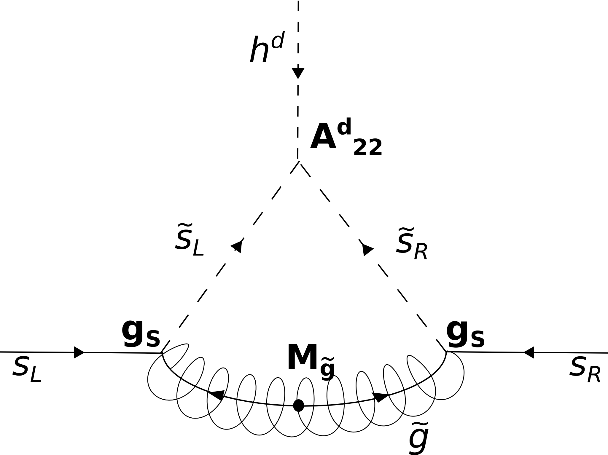
(a)

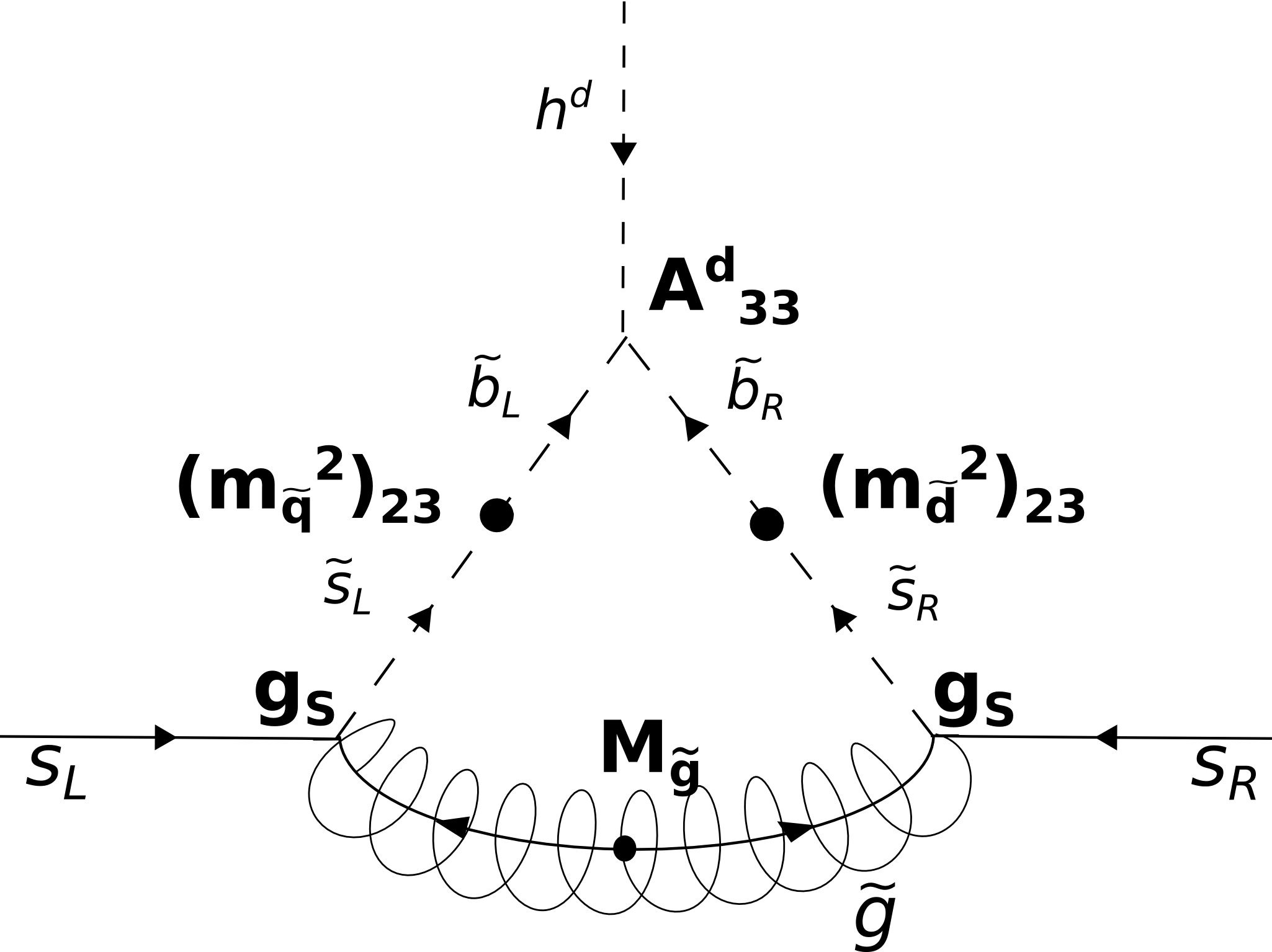
(b)

Figure 1: Examples of diagrams that describe threshold corrections to the strange Yukawa coupling at $\mu_{\rm sp}$. (a) the flavour-diagonal leading gluino diagram; (b) possibly an even bigger contribution arising in the case of flavour mixing in the soft-mass matrix.

The situation changes when non-zero off-diagonal soft mass entries are allowed (see the right panel of Fig. 1). In such a case, the dominant GFV contribution to the strange quark self-energy associated with a gluino loop [11] can be written as

$$(\Sigma^{d}_{22})^{\tilde{g}}=\frac{\alpha_{s}}{6\pi}m_{\tilde{g}}v_{d}(A^{d}_{33}-Y_{b}\mu\tan\beta)\,S\,\sin 2\theta_{\tilde{q}}\,\sin 2\theta_{\tilde{d}}\!\sum_{m,n=2,3}(-1)^{n+m}C_{0}({m_{\tilde{g}}}^{\!\!\!2},m^{2}_{\tilde{q}^{L}_{m}},m^{2}_{\tilde{d}^{R}_{n}}),$$ (10)

where $S={\rm sgn}\left[\left(m^{2}_{\tilde{q}^{L}_{2}}-m^{2}_{\tilde{q}^{L}_{3}}\right)\left(m^{2}_{\tilde{d}^{R}_{2}}-m^{2}_{\tilde{d}^{R}_{3}}\right)\right]$, and

$$\sin 2\theta_{\tilde{q}}\,=\,\frac{2(m^{2}_{\tilde{q}})_{23}}{\sqrt{\left[(m_{\tilde{q}}^{2})_{22}-(m^{2}_{\tilde{q}})_{33}\right]^{2}+4((m^{2}_{\tilde{q}})_{23})^{2}}},\hskip 14.22636pt\sin 2\theta_{\tilde{d}}\,=\,\frac{2(m^{2}_{\tilde{d}})_{23}}{\sqrt{\left[(m^{2}_{\tilde{d}})_{22}-(m^{2}_{\tilde{d}})_{33}\right]^{2}+4((m^{2}_{\tilde{d}})_{23})^{2}}}.$$

Here, we have assumed that $(m^{2}_{\tilde{q}})_{23}$ and $(m^{2}_{\tilde{d}})_{23}$ are the only non-zero off-diagonal elements of the down-squark mass matrix, and that they are real. It follows from Eq. (10) that chirality-conserving GFV interactions  $[(m^{2}_{\tilde{q}})_{23}\,\tilde{s}_{L}^{*}\tilde{b}_{L}+{\rm h.c.}]$  and  $[(m^{2}_{\tilde{d}})_{23}\,\tilde{s}_{R}^{*}\tilde{b}_{R}+{\rm h.c.}]$  generate a threshold correction to $Y_{s}$ of the order of $\Delta Y_{s}\sim\alpha_{s}A_{33}^{d}/M_{\rm SUSY}$, which in general can be large enough to facilitate Yukawa coupling unification for the second family, even when the coupling $A_{22}^{d}$ is small.

The above description, however, should be treated only as a simplified qualitative illustration. In a general case, also other off-diagonal elements of the squark mass matrix can significantly differ from zero, which renders mixing among all the three generations important. To make sure that all such effects are properly taken into account, in the following we turn to a full numerical analysis.

3 Impact of the GFV threshold corrections on Yukawa unification

Let us start this section with briefly describing the numerical tools and procedures employed to identify the GFV $SU(5)$ GUT parameter space regions where the Yukawa coupling unification becomes possible. Next, we shall perform a numerical scan and use its results to determine those SUSY parameters whose non-zero values are indispensable from the point of view of the considered unification.

3.1 Numerical tools and scanning methodology

Points satisfying the Yukawa coupling unification conditions at the ${\rm GUT}$ scale are found by scanning the parameter space of the model defined in Sec. 3.2. To this end, we use the numerical package BayesFITSv3.2 that was first developed in Ref. [25] and modified to incorporate the full GFV structure of the soft SUSY-breaking sector in Ref. [23]. The package uses for sampling MultiNest v2.7 [26] which allows a fast and efficient scanning according to a predefined likelihood function. The likelihood corresponding to the $SU(5)$ boundary condition (5) is modeled with a Gaussian distribution as follows,

$$\mathcal{L}_{\rm Yuk}=\sum_{i=1,2,3}\exp\left[-(1-Y^{e}_{ii}(M_{\textrm{GUT}})/Y^{d}_{ii}(M_{\textrm{GUT}}))^{2}/2\sigma_{\rm Yuk}^{2}\right],$$ (11)

and the allowed deviation from the exact unification condition, $\sigma_{\rm Yuk}$, is set to 5%.

$m_{t}^{\rm pole}$		$m_{b}^{\overline{MS}}(m_{b})$		$\alpha_{s}^{\overline{MS}}(M_{Z})$		$\alpha_{\mathrm{em}}^{-1}(M_{Z})$
$173.34\pm 0.76$ GeV		$4.18\pm 0.03$ GeV		$0.1184\pm 0.0007$		$127.944\pm 0.015$
$m_{u}^{\overline{MS}}$	$m_{d}^{\overline{MS}}$	$m_{s}^{\overline{MS}}$	$m_{c}^{\overline{MS}}(m_{c})$	$m_{e}^{\rm pole}$	$m_{\mu}^{\rm pole}$	$m_{\tau}^{\rm pole}$	$M_{Z}^{\rm pole}$
2.3 MeV	4.8 MeV	95 MeV	1.275 GeV	511 keV	106 MeV	1.777 GeV	91.19 GeV
$\bar{\rho}$		$\bar{\eta}$		$A$		$\lambda$
$0.159\pm 0.045$		$0.363\pm 0.049$		$0.802\pm 0.020$		$0.22535\pm 0.00065$

Table 1: Standard Model parameters [28, 29] used in our numerical calculations. The light ($u$, $d$, $s$) quark masses are $\overline{\rm MS}$-renormalized at 2 GeV.

Mass spectra are calculated with SPheno v3.3.3 [27]. The choice is dictated by the fact that at the moment SPheno is the only SUSY spectrum generator where the full flavour structure of threshold corrections to the Yukawa couplings, as given in Ref. [11], is implemented. As is the case of other tools of this kind, the renormalization group equations of the MSSM are solved by an iterative algorithm that interpolates between different scales at which the parameters are defined. The boundary with the SM (i.e. the scale $\mu_{\rm sp}$) is set at $M_{Z}$.

Four SM parameters ($m_{t}^{\rm pole}$, $m_{b}^{\overline{MS}}(m_{b})$, $\alpha_{\mathrm{em}}^{-1}(M_{Z})$ and $\alpha_{s}^{\overline{MS}}(M_{Z})$) are treated as nuisance parameters and randomly drawn from a Gaussian distribution centred around their experimentally measured central values [28]. The elements of the CKM matrix in the Wolfenstein parametrisation ($\bar{\rho}$, $\bar{\eta}$, $A$, $\lambda$) are scanned as well, with central values and errors given by the UTfit Collaboration for the scenario allowing new physics effects in loop observables [29]. The other SM parameters which are passed as an input to SPheno ($m_{s}^{\overline{MS}}$, $m_{c}^{\overline{MS}}(m_{c})$, $m_{d}^{\overline{MS}}$, $m_{u}^{\overline{MS}}$, $m_{\tau}^{\rm pole}$, $m_{\mu}^{\rm pole}$, $m_{e}^{\rm pole}$, $M_{Z}^{\rm pole}$) are fixed at their experimentally measured values. Our SM input is collected in Table 1.

3.2 Input SUSY parameters

We start our analysis by defining a general set of SUSY parameters at the GUT scale. Since a priori we do not know which GFV parameters in the down-squark sector are indispensable to achieve the Yukawa coupling unification and which can be skipped, initially we allow all of them to assume non-zero values. The aim of the numerical scan is to identify those parameters that are essential.

We assume for simplicity that all the soft SUSY-breaking parameters are real, therefore neglecting the possibility of new SUSY sources of CP violation. The GUT-scale $SU(5)$ boundary conditions for the soft-masses read

$$(m^{2}_{\tilde{l}})_{ij}=(m^{2}_{\tilde{d}})_{ij}\equiv(m^{2}_{dl})_{ij},\qquad(m^{2}_{\tilde{q}})_{ij}=(m^{2}_{\tilde{u}})_{ij}=(m^{2}_{\tilde{e}})_{ij}\equiv(m^{2}_{ue})_{ij}.$$ (12)

We do not impose any additional conditions on the relative magnitudes of the diagonal entries. In particular, both normal and inverted hierarchies for the elements $(m^{2}_{dl})_{ii}$ and $(m^{2}_{ue})_{ii}$ are allowed. The off-diagonal elements of the down-squark matrix are normalized to the entry $(m^{2}_{dl})_{33}$, and are required to satisfy the upper limit $(m^{2}_{dl})_{ij}/(m^{2}_{dl})_{33}\leq 1$.

We further assume that

$$(m^{2}_{ue})_{ij}=0,\;\;i\neq j.$$ (13)

Such an assumption is not expected to cause any significant loss of generality because relatively large off-diagonal elements of $(m^{2}_{\tilde{q}})_{ij}$ are generated radiatively at $M_{\rm SUSY}$ due to the RGE running in the super-CKM basis. We restrict our study to the case $(m^{2}_{dl})_{ij}>0$, as it is a desired property for the Yukawa unification. At this point we are allowed to introduce a short-hand notation

$$m^{dl}_{ij}\equiv\sqrt{(m^{2}_{dl})_{ij}},\qquad m^{ue}_{ij}\equiv\sqrt{(m^{2}_{ue})_{ij}}.$$ (14)

The GUT-scale $SU(5)$ boundary conditions for the trilinear terms are given by

$$A_{ij}^{d}=A_{ji}^{e}\equiv A_{ij}^{de}.$$ (15)

We constrain the relative magnitude of the diagonal entries by the corresponding Yukawa couplings

$$\frac{|A^{f}_{ii}|}{|A^{f}_{33}|}<\frac{Y^{f}_{ii}}{Y^{f}_{33}}.$$ (16)

We do so because we aim at relaxing the strong tension between the EW vacuum stability condition and Yukawa unification that has been observed [10] in the case of large diagonal $A$-terms. We also impose that

$$A^{u}_{ij}=0,\;\;i\neq j.$$ (17)

On the other hand, the off-diagonal entries in the down-sector trilinear matrix are not constrained in our initial scan to scale proportionally to the corresponding Yukawa matrix entries. The are only required to satisfy $|(A^{de}_{ij})/(A^{de}_{33})|\leq 0.5$.

Finally, we assume that the gaugino mass parameters are universal at $M_{\rm GUT}$,

$$M_{1}=M_{2}=M_{3}\equiv M_{1/2},$$ (18)

which is the simplest among relations that naturally arise in the framework of SUSY $SU(5)$ GUTs. The sign of the parameter $\mu$ is chosen to be negative to facilitate the second family unification, as explained in Sec. 2.

Parameter	Scanning Ranges: $GFV_{23}$	Scanning Ranges: $GFV_{123}$
$M_{1/2}$	[$100$, $4000$] $\,\mathrm{GeV}$	[$100$, $4000$] $\,\mathrm{GeV}$
$m_{H_{u}}$	[$100$, $8000$] $\,\mathrm{GeV}$	[$100$, $8000$] $\,\mathrm{GeV}$
$m_{H_{d}}$	[$100$, $8000$] $\,\mathrm{GeV}$	[$100$, $8000$] $\,\mathrm{GeV}$
$\tan\beta$	[$3$, $45$]	[$3$, $45$]
$\rm{sgn}\,\mu$	$-1$	$-1$
$A_{33}^{de}$	[$0$, $5000$] $\,\mathrm{GeV}$	[$0$, $5000$] $\,\mathrm{GeV}$
$A_{33}^{u}$	[$-9000$, $9000$] $\,\mathrm{GeV}$	[$-9000$, $9000$] $\,\mathrm{GeV}$
$A^{de}_{11}/A^{de}_{33}$	[$-0.00028$, $0.00028$]	[$-0.00028$, $0.00028$]
$A^{de}_{22}/A^{de}_{33}$	[$-0.065$, $0.065$]	[$-0.065$, $0.065$]
$A^{u}_{22}/A^{u}_{33}$	[$-0.005$, $0.005$]	[$-0.005$, $0.005$]
$A^{de}_{ij}/A^{de}_{33},\;i\neq j$	$0$	[$-0.5$, $0.5$]
$m_{ii}^{dl},\;i=1,2,3$	[$100$, $10000$] $\,\mathrm{GeV}$	[$100$, $7000$] $\,\mathrm{GeV}$
$m^{dl}_{23}/m^{dl}_{33}$	[$0$, $1$]	[$0$, $1$]
$m^{dl}_{13}/m^{dl}_{33}$	$0$	[$0$, $1$]
$m^{dl}_{12}/m^{dl}_{33}$	$0$	[$0$, $1$]
$m_{ii}^{ue},\;i=1,2,3$	[$100$, $7000$] $\,\mathrm{GeV}$	[$100$, $7000$] $\,\mathrm{GeV}$

Table 2: Ranges of the input SUSY parameters used in our initial scan. Several omitted soft SUSY-breaking parameters at the GUT scale (namely $A^{u}_{11}$ as well as $A^{u}_{ij}$ and $m^{ue}_{ij}$ for $i\neq j$) have been set to zero.

In our study, we consider two different scenarios for the Yukawa matrix unification:
$GFV_{23}$: Only the third and the second generation Yukawa couplings are unified at the ${\rm GUT}$ scale. The only relevant GFV parameter in this case is $m^{dl}_{23}$.
$GFV_{123}$: Yukawa couplings of all the three families are unified at the ${\rm GUT}$ scale. All the GFV parameters in the down-squark sector can assume non-zero values.
In Table 2, we collect the scanning ranges for our initial set of the input SUSY parameters. In the next subsection, we shall identify those being particularly relevant from the point of view of the Yukawa coupling unification.

3.3 Yukawa unification through flavour-violating terms

3.3.1 $\boldsymbol{GFV_{23}}$: unification of the third and second family

The performed scan has returned the MSSM spectrum for 121986 parameter-space points, among which 34758 yield the Yukawa couplings of leptons and down-type quarks at $M_{\textrm{GUT}}$ equal within 10% for the second and third generations.

In Fig. 2, we present distributions of the collected points in the planes of ($m^{dl}_{23}/m^{dl}_{33}$, $Y_{b}\mu\tan\beta$) (a), ($M_{1/2}$, $Y_{b}\mu\tan\beta$) (b), and ($\tan\beta$, $A^{de}_{33}$) (c). All the points that satisfy the Yukawa unification condition for the third generation at $2\sigma$ ($0.9<Y_{b}/Y_{\tau}<1.1$) are represented as gray stars. Those for which both third and second generations are unified at $2\sigma$ are shown as green dots.

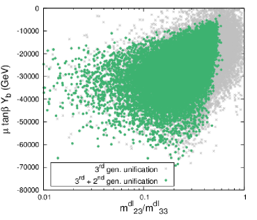
(a)

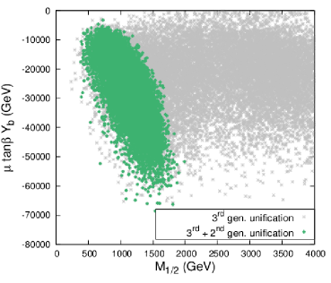
(b)

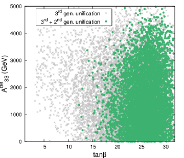
(c)

Figure 2: Scatter plot of the $GFV_{23}$ points in the planes ($m^{dl}_{23}/m^{dl}_{33}$, $Y_{b}\mu\tan\beta$) (a), ($M_{1/2}$, $Y_{b}\mu\tan\beta$) (b), and ($\tan\beta$, $A^{de}_{33}$) (c). Gray stars: all points satisfying the Yukawa unification condition for the third generation at $2\sigma$; green dots: points for which both heavier generations are unified at $2\sigma$.

The most characteristic feature of the $GFV_{23}$ scenario is the lack of points consistent with the Yukawa unification and with a large universal gaugino mass parameter, $M_{1/2}>2000\,\mathrm{GeV}$. This is a straightforward consequence of Eq. (10) in which the gluino mass appears both as a multiplicative factor and through the loop function $C_{0}$. The impact of the latter is of particular importance since for $M_{1/2}>2000\,\mathrm{GeV}$, and for the fixed sfermion masses, it leads to strong suppression of the threshold correction $(\Sigma^{d}_{22})^{\tilde{g}}$. At the same time, the correction is somewhat enhanced when the mass of sfermions is decreased with a fixed $M_{1/2}$, although this effect is less prominent.

Secondly, the strange-muon unification occurs for both large and small values of $A^{de}_{33}$, which is of relevance for the minimisation of the scalar potential, as further discussed in Sec. 4.2.4. This is confirmed by panels (a) and (b) of Fig. 2 where the values of another relevant factor $Y_{b}\mu\tan\beta$, which appears in Eq. (10), are depicted for all the model points satisfying the Yukawa unification condition. One can observe, by comparing with panel (c) of Fig. 2, that $|Y_{b}\mu\tan\beta|\gg A^{de}_{33}$ and the impact of $A^{de}_{33}$ in Eq. (10) is indeed negligible.

This means that the threshold correction $(\Sigma^{d}_{22})^{\tilde{g}}$ essentially depends on three parameters: the gluino mass, the off-diagonal element $m^{dl}_{23}$, and the higgsino mass term $\mu$. As a consequence, the strange-muon Yukawa coupling unification can be achieved through an interplay of several mechanisms. For small gluino masses (that correspond to the upper-left corner of Fig. 2(b)), the threshold correction $(\Sigma^{d}_{22})^{\tilde{g}}$ can be enhanced either by large values of the GFV parameter $m^{dl}_{23}$ (upper-right corner of Fig. 2(a)) or by large values of the factor $Y_{b}\mu\tan\beta$ with $m^{dl}_{23}$ as small as $0.01$. The latter effect is additionally enhanced for moderate values of $\tan\beta$ which are preferred in the $GFV_{23}$ scenario, as shown in panel (c) of Fig. 2.

For large gluino masses, that correspond to $M_{1/2}\geq 1500$ $\,\mathrm{GeV}$, the threshold correction of Eq. (10) becomes suppressed by the loop function $C_{0}$. Therefore, both large $m^{dl}_{23}$ and an even larger $\mu$-term are needed to achieve Yukawa unification for the second family.

Finally, in the squark and slepton sector, the $GFV_{23}$ scenario favours a spectrum with the third generation much heavier than the first two ones. It has important phenomenological consequences for the dark matter and flavour observables, as discussed in Sec. 4.2.

3.3.2 $\boldsymbol{GFV_{123}}$: unification of all three families

We collected about $1.5\times 10^{5}$ points through our scanning procedure of the parameter space defined in Table 2.

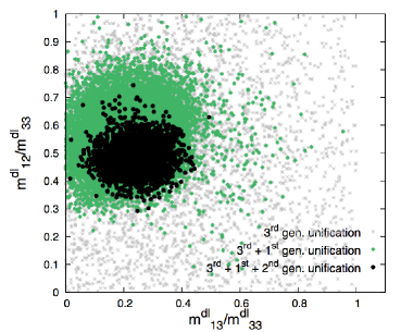
(a)

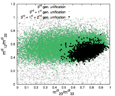
(b)

Figure 3: Scatter plot of the $GFV_{123}$ points in the planes ($m^{dl}_{13}/m^{dl}_{33}$, $m^{dl}_{12}/m^{dl}_{33}$) (a), and ($m^{dl}_{23}/m^{dl}_{33}$, $m^{dl}_{12}/m^{dl}_{33}$) (b). Gray stars: all the points satisfying the Yukawa unification condition for the third generation at $2\sigma$; green diamonds: points additionally requiring $2\sigma$ unification of the first family; black dots: points for which all the three generations are unified at $2\sigma$.

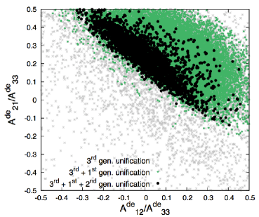
(a)

(b)

(c)

Figure 4: Scatter plot of the $GFV_{123}$ points in the planes ($A^{de}_{12}/A^{de}_{33}$, $A^{de}_{21}/A^{de}_{33}$) (a), ($A^{de}_{13}/A^{de}_{33}$, $A^{de}_{31}/A^{de}_{33}$) (b), and ($A^{de}_{23}/A^{de}_{33}$, $A^{de}_{32}/A^{de}_{33}$) (c). The colour code is the same as in Fig. 3.

In Fig. 3, we present distributions of points in the planes ($m^{dl}_{13}/m^{dl}_{33}$, $m^{dl}_{12}/m^{dl}_{33}$) (a) and ($m^{dl}_{23}/m^{dl}_{33}$, $m^{dl}_{13}/m^{dl}_{33}$) (b). All the points that satisfy the Yukawa unification condition for the third generation at $2\sigma$ are depicted as gray stars (they account for $49\%$ of all the points), while those that additionally fulfil $2\sigma$ unification of the first family as green diamonds ($29\%$ of all the points). Finally, black dots correspond to those points for which all three generations are unified at $2\sigma$ ($1.7\%$ of all the points collected by the scan). In Fig. 4, similar distributions are shown for the flavour-violating entries of the trilinear down-sector matrix, in the planes corresponding to ($A^{de}_{12}/A^{de}_{33}$, $A^{de}_{21}/A^{de}_{33}$) (a), ($A^{de}_{13}/A^{de}_{33}$, $A^{de}_{31}/A^{de}_{33}$) (b), and ($A^{de}_{23}/A^{de}_{33}$, $A^{de}_{32}/A^{de}_{33}$) (c).

Several observations can now be made. First of all, it is known that satisfactory unification of the third family Yukawa couplings is quite easy to achieve in the Minimal Flavour Violating $SU(5)$ for moderate values of $\tan\beta$. This is confirmed by both Fig. 3 and Fig. 4 where gray points can easily be found for vanishing flavour-violation in the GUT-scale soft parameters.

Secondly, the functional form of the threshold correction in Eq. (10) might suggest that non-zero soft-mass elements $m^{dl}_{23}$ and $m^{dl}_{13}$ are sufficient to allow the Yukawa unification in both the second and first family cases. Such a simplistic picture, however, is not true, as can be seen from the panel (a) of Fig. 3 where large $m^{dl}_{12}$ is clearly favoured. To understand what happens, let us note that the GFV corrections $(\Sigma^{d}_{22})^{\tilde{g}}$ and $(\Sigma^{d}_{11})^{\tilde{g}}$ (obtained from Eq. (10) by replacing indices “2” with “1”) are determined by overlapping sets of parameters, in particular $M_{1/2}$ and $A_{33}^{de}$. On the other hand, sizes of those corrections as required by the Yukawa coupling unification differ by two orders of magnitude. Let us now assume that $(\Sigma^{d}_{11})^{\tilde{g}}$ is fixed by the unification condition for the first family. Thus $M_{1/2}$ and $A_{33}^{de}$, already constrained by unification of the third family, are even more limited. With such a choice of parameters, however, the correction $(\Sigma^{d}_{22})^{\tilde{g}}$ is still too small to allow unification of the second family, and needs to be further enhanced by another contribution. Such a contribution comes from a diagram like the one shown in Fig. 1(b), but with the trilinear term $A_{21}^{de}$ in the vertex and $m^{dl}_{12}$ mixing in the right-handed sector. However, a similar diagram also exists for the first family, and the corresponding contribution should be added to the one driven by $m^{dl}_{13}$. That explains why all the five parameters $m^{dl}_{12}$, $m^{dl}_{13}$, $m^{dl}_{23}$, $A_{12}^{de}$ and $A_{21}^{de}$ must be adjusted simultaneously. Note also that $A_{12/21}^{de}$ can be kept relatively low, as this contribution is always enhanced by a large value of $m^{dl}_{12}$.

(a)

(b)

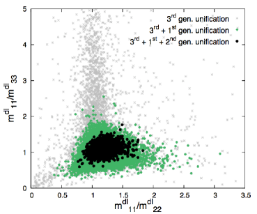
(c)

Figure 5: Scatter plot of the $GFV_{123}$ points in the planes ($M_{1/2}$, $A^{d}_{33}$) (a), ($m_{H_{d}}/m_{H_{u}}$, $\tan\beta$) (b), and ($m^{dl}_{11}/m^{dl}_{22}$, $m^{dl}_{11}/m^{dl}_{33}$) (c). The colour code is the same as in Fig. 3.

Flavour-violating parameters are not the only ones constrained by the Yukawa unification condition. In Fig. 5, we present distributions of points in the planes ($M_{1/2}$, $A^{de}_{33}$) (a), ($m_{H_{d}}/m_{H_{u}}$, $\tan\beta$) (b), and ($m^{dl}_{11}/m^{dl}_{22}$, $m^{dl}_{11}/m^{dl}_{33}$) (c). The colour code is the same as in Fig. 3. One can observe that values of both $M_{1/2}$ and $A^{d}_{33}$ need to be very limited in order to facilitate unification in the first and second family cases, as they directly enter Eq. (10). The ratio $m_{H_{d}}/m_{H_{u}}$ in the range $[0-2]$ allows the unification of the second family for larger values of $\tan\beta$, $\tan\beta\in[15-25]$. Finally, large mass splittings between the diagonal entries of the down-squark mass matrix are disfavoured because they would lead to a strong suppression of SUSY threshold corrections, as can be deduced from Eq. (10).

We conclude this section with summarising the allowed ranges of the non-zero GFV parameters that characterise the $SU(5)$ GUT scenario with the full Yukawa coupling unification:

$$0.5<m^{dl}_{23}/m^{dl}_{33}<1, \quad 0<m^{dl}_{13}/m^{dl}_{33}<0.5, \quad 0.3<m^{dl}_{12}/m^{dl}_{33}<0.7,$$

$$0<A^{d}_{12}/A^{d}_{33}<0.2, \quad 0<A^{d}_{21}/A^{d}_{33}<0.2.$$ (19)

4 Phenomenology of the unification scenarios

So far we have discussed the possibility of satisfying the $SU(5)$ boundary conditions for the Yukawa couplings by allowing a non-trivial flavour structure of the soft terms at the ${\rm GUT}$ scale. In this section, we will discuss compatibility of the results obtained in Sec. 3 with various phenomenological constraints. First, we are going to consider a set of experimental measurements from the dark matter searches, Higgs physics, flavour physics and EW precision measurements. Next, theoretical limits provided by the EW vacuum stability requirement will be taken into account. In this exposition, we do not aim at finding the best possible fit of the MSSM to the experimental data. Rather, we show that the Yukawa unification requirement does not contradict consistency of the MSSM with observations.

4.1 Experimental constraints

In order to find points satisfying both the Yukawa coupling unification conditions at the GUT scale and the experimental constraints, we use the tools described in Sec. 3.1, and scan the parameter space of the unification scenarios given in Table 3. The experimental constraints applied in the analysis are listed in Table 4.

Parameter	Scanning Ranges: $GFV_{23}$	Scanning Ranges: $GFV_{123}$
$M_{1/2}$	[$100$, $2000$] $\,\mathrm{GeV}$	[$200$, $1100$] $\,\mathrm{GeV}$
$m_{H_{u}}$, $m_{H_{d}}$	[$100$, $8000$] $\,\mathrm{GeV}$	[$100$, $8000$] $\,\mathrm{GeV}$
$\tan\beta$	[$3$, $35$]	[$3$, $25$]
$\rm{sgn}\,\mu$	$-1$	$-1$
$A_{33}^{de}$	[$0$, $5000$] $\,\mathrm{GeV}$	[$400$, $1100$] $\,\mathrm{GeV}$
$A_{33}^{u}$	[$-9000$, $9000$] $\,\mathrm{GeV}$	[$-9000$, $9000$] $\,\mathrm{GeV}$
$A^{de}_{11}/A^{de}_{33}$	[$-0.00028$, $0.00028$]	[$-0.00028$, $0.00028$]
$A^{de}_{22}/A^{de}_{33}$	[$-0.065$, $0.065$]	[$-0.065$, $0.065$]
$A^{u}_{22}/A^{u}_{33}$	[$-0.005$, $0.005$]	[$-0.005$, $0.005$]
$A^{de}_{12}/A^{de}_{33}$,  $A^{de}_{21}/A^{de}_{33}$	$0$	[$-0.2$, $0.2$]
$m_{ii}^{dl},\;i=1,2,3$	[$100$, $10000$] $\,\mathrm{GeV}$	[$100$, $7000$] $\,\mathrm{GeV}$
$m^{dl}_{23}/m^{dl}_{33}$	[$0.0$, $0.4$]	[$0.5$, $1.0$]
$m^{dl}_{13}/m^{dl}_{33}$	$0$	[$0.0$, $0.5$]
$m^{dl}_{12}/m^{dl}_{33}$	$0$	[$0.3$, $0.7$]
$m_{ii}^{ue},\;i=1,2,3$	[$100$, $7000$] $\,\mathrm{GeV}$	[$100$, $7000$] $\,\mathrm{GeV}$

Table 3: Ranges of the input SUSY parameters in the GFV $SU(5)$ scenario with Yukawa coupling unification. Several parameters that are not explicitly listed in the table (namely $A^{u}_{11}$, $A^{u}_{ij}$ and $m^{ue}_{ij}$ for $i\neq j$, $A^{de}_{23/32}$, $A^{de}_{13/31}$) have been set to zero.

All the flavour observables have been evaluated with the code SUSY_FLAVOR v2.10 [30]. It calculates the renormalized Yukawa matrices in the MSSM and derives the correct CKM matrix as described in Ref. [11]. Apart from the $B$-meson mass differences $\Delta M_{B_{d}}$ and $\Delta M_{B_{s}}$, we also consider their ratio $\Delta M_{B_{d}}/\Delta M_{B_{s}}$ for which more precise lattice inputs are available [31, 32]. Theory uncertainties in the cases of $\rm BR\left(\overline{B}\rightarrow X_{s}\gamma\right)$, ${\rm BR}(B_{s(d)}\to\mu^{+}\mu^{-})$ and $|\epsilon_{K}|$ have been estimated following Refs. [33],  [34], and [35], respectively. In the latter case, they arise mainly from poor convergence of the QCD perturbation series for double charm contributions. Errors stemming from the Wolfenstein parameters $\rho$ and $\eta$ are not taken into account in the third column of Table 4. Each point of our scan corresponds to a particular value of $(\rho,\eta)$, and it is tested against SUSY-sensitive loop observables that matter for determining allowed regions in the $(\rho,\eta)$ plane. At the same time, the considered values of all the CKM parameters are within the ranges allowed by tree-level observables. We use the same code to determine the values of the Lepton Flavour Violating observables.

The relic density and the spin-independent neutralino-proton cross section $\sigma^{\rm SI}_{p}$ have been calculated with the help of DarkSUSY v5.0.6 [36]. For the EW precision constraints FeynHiggs v2.10.0 [37, 38, 39, 40] has been used. To include the exclusion limits from Higgs boson searches at LEP, Tevatron, and LHC, as well as the $\chi^{2}$ contributions from the Higgs boson signal rates from Tevatron and LHC, we applied HIGGSBOUNDS v4.0.0 [41, 42, 43] interfaced with HIGGSSIGNALS v1.0.0 [44].

Measurement	Mean or range	Error [ exp., th.]	Reference
$\Omega_{\chi}h^{2}$	$0.1199$	[$0.0027$, $10\%$]	[48]
LUX (2013)	See Sec. 3 of [47]	See Sec. 3 of [47]	[45]
$m_{h}$ (by CMS)	$125.7\,\mathrm{GeV}$	[$0.4$, $3.0$] $\,\mathrm{GeV}$	[49]
LHC $\sqrt{s}=8\,\mathrm{TeV}$	Sec. 4.2.3	Sec. 4.2.3	[52, 53, 54]
$\sin^{2}\theta_{\mathrm{eff}}$	$0.23155$	[$0.00012$, $0.00015$]	[28]
$M_{W}$	$80.385\,\mathrm{GeV}$	[$0.015$, $0.015$] $\,\mathrm{GeV}$	[28]
$\rm BR\left(\overline{B}\rightarrow X_{s}\gamma\right)$$\times 10^{4}$	$3.43$	[$0.22$, $0.23$]	[32]
$\rm BR\left(B_{s}\to\mu^{+}\mu^{-}\right)\times 10^{9}$	$2.8$	[$0.7$, $0.23$]	[50]
$\rm BR\left(B_{d}\to\mu^{+}\mu^{-}\right)\times 10^{10}$	$3.9$	[$1.6$, $0.09$]	[50]
$\Delta M_{B_{s}}\times 10^{11}$	$1.1691\,\mathrm{GeV}$	[$0.0014$, $0.1580$] $\,\mathrm{GeV}$	[28]
$\Delta M_{B_{d}}\times 10^{13}$	$3.357\,\mathrm{GeV}$	[$0.033$, $0.340$] $\,\mathrm{GeV}$	[28]
$\Delta M_{B_{d}}/\Delta M_{B_{s}}\times 10^{2}$	$2.87$	[$0.02$, $0.14$]	[32]
$\sin(2\beta)_{\rm exp}$	$0.682$	[$0.019$, $0.003$]	[28]
$\rm BR\left(B_{u}\rightarrow\tau\nu\right)$$\times 10^{4}$	$1.14$	[$0.27$, $0.07$]	[28]
$\textrm{BR}(K^{+}\to\pi^{+}\nu\bar{\nu})\times 10^{10}$	$1.73$	[$1.15,0.04$]	[28]
$\epsilon_{K}\times 10^{3}$	$2.228$	[$0.011$, $0.17$]	[28]
$|d_{n}|\times 10^{26}$	< $2.9$ $e$ cm	[$0$, $30\%$]	[51]
$\rm BR\left(\mu^{+}\to e^{+}\gamma\right)$$\times 10^{13}$	< $5.7$	[0,0]	[55]
$\rm BR\left(\tau^{\pm}\to e^{\pm}\gamma\right)$$\times 10^{8}$	< $3.3$	[0,0]	[56]
$\rm BR\left(\tau^{\pm}\to\mu^{\pm}\gamma\right)$$\times 10^{8}$	< $4.4$	[0,0]	[56]
$\rm BR\left(\mu^{+}\to e^{+}e^{+}e^{-}\right)$$\times 10^{12}$	< $1.0$	[0,0]	[57]
$\rm BR\left(\tau^{\pm}\to e^{\pm}e^{+}e^{-}\right)$$\times 10^{8}$	< $2.7$	[0,0]	[58]
$\rm BR\left(\tau^{\pm}\to\mu^{\pm}\mu^{+}\mu^{-}\right)$$\times 10^{8}$	< $2.1$	[0,0]	[58]

Table 4: The experimental constraints applied in the analysis.

In all the cases, the likelihood for positive experimental measurements was modeled with Gaussian distribution, while for upper bounds – with half-Gaussian one. The likelihood relative to the LUX results [45] was calculated by closely following the procedure first developed in Ref. [46] and described in Sec. 3 of Ref. [47]. The likelihood for the LHC direct SUSY searches was not included in the global likelihood used by MultiNest. Our treatment of this constraint will be described in Sec. 4.2.3. We collected in total about $2.1\times 10^{5}$ points.

4.2 $\boldsymbol{GFV_{23}}$: unification of the third and second family

4.2.1 Dark matter

Relic abundance of the dark matter in GUT-constrained SUSY scenarios is usually the most stringent constraint. It is well known that properties of the DM candidate strongly depend on its composition. In the almost purely bino case, the relic density is generally too large, and the annihilation cross-section needs to be enhanced by some mechanism, usually by co-annihilation with the lightest sfermion, or resonance annihilation through one of the Higgs bosons. On the other hand, a significant higgsino component of the lightest neutralino opens a possibility of efficient annihilation into gauge bosons through a $t$-channel exchange of higgsino-like $\tilde{{\chi}}^{\pm}_{1}$ and $\tilde{{\chi}}^{0}_{2}$. In fact, the annihilation cross-section in such a case is usually too large, which leads to DM underabundance.

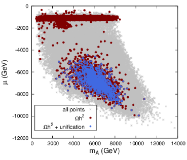
(a)

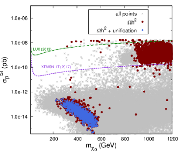
(b)

Figure 6: Scatter plot of the $GFV_{23}$ points in the planes ($m_{A}$, $\mu$) (a) and ($m_{\tilde{\chi}^{0}_{1}}$, $\sigma^{\rm SI}_{p}$) (b). Gray stars: all points collected by the scan; brown dots: points satisfying the DM relic density constraint at $3\sigma$; blue diamonds: points for which additionally the Yukawa unification of the second an third family holds. The meaning of dashed lines is described in the text.

In Fig. 6, we present distributions of points found by our scanning procedure in the planes ($m_{A}$, $\mu$) (a) and ($m_{\tilde{\chi}^{0}_{1}}$, $\sigma^{\rm SI}_{p}$) (b). All the points collected by the scan are depicted as gray stars, while those that satisfy at $3\sigma$ the experimental constraint on the DM relic density appear as brown dots. Blue diamonds correspond to those scenarios for which additionally the Yukawa coupling unification holds. The green dashed line indicates the $90\%$ C.L. exclusion bound on the $\sigma^{\rm SI}_{p}$ based on the 85-day measurement by the LUX collaboration [45], while the purple dashed line is a projection of XENON1T sensitivity [59]. By comparing panels (a) and (b) of Fig. 6 one can see that in the region where Yukawa unification is achieved, the neutralino LSP is bino-like, which corresponds to a relatively low spin-independent proton-neutralino cross-section. In other words, the condition of Yukawa coupling unification strongly disfavours purely or partly higgsino-like neutralino. This is due to the fact that only the points with $|\mu|\mathrel{\hbox to0.0pt{\lower 4.0pt\hbox{\hskip 1.0pt$\sim$}\hss}\raise 1.0pt\hbox{$<$}}1\,\mathrm{TeV}$ in Fig. 6(a) correspond to a significant higgsino component of the LSP. In such a case, the $\mu$-dependent contribution in Eq. (10) is too small to allow for unification of the second family Yukawa couplings. Thus, it is an important phenomenological signature of the GFV $SU(5)$ Yukawa unification scenario with the universal gaugino masses that only bino-like neutralino is allowed.

A unique mechanism that makes the effective increase of the DM annihilation cross-section possible in this case is the neutralino co-annihilation with the lightest sneutrino. The pseudoscalar is too heavy to allow for resonant $\tilde{\chi}^{0}_{1}$ annihilation (as can be read from the panel (a) of Fig. 6), while the masses of the coloured sfermions in the GUT-constrained unification scenarios are always larger than those of the sleptons. It is due to a renormalization effect, as their RGE running is strongly driven by the gluino. Such a property of the spectrum, however, has important consequences for experimental testability. In Fig. 6(b) the dashed lines indicate the present reach and the expected sensitivity for LUX and XENON1T. The region favoured by the relic density constraint in the Yukawa unification scenario remains far beyond the reach for any of them. On the other hand, spectra characterized by the presence of a light bino-like $\tilde{\chi}^{0}_{1}$ and a sneutrino close in mass are already being tested by the LHC $\sqrt{s}=8\,\mathrm{TeV}$, as will be discussed in Sec. 4.2.3. It is an interesting aspect of the $GFV_{23}$ Yukawa unification scenario that the requirement of satisfying the DM relic density constraint makes it testable by the LHC $\sqrt{s}=14\,\mathrm{TeV}$ run.

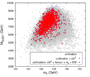
(a)

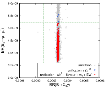
(b)

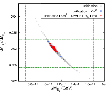
(c)

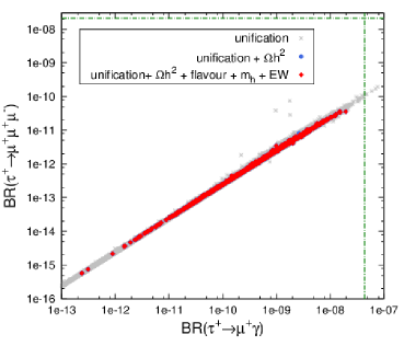
(d)

Figure 7: Scatter plot of the $GFV_{23}$ points in the planes ($m_{h}$, $M_{\rm SUSY}$) (a), ($\rm BR\left(\overline{B}\rightarrow X_{s}\gamma\right)$, $\rm BR\left(B_{s}\to\mu^{+}\mu^{-}\right)$) (b), ($\Delta M_{B_{s}}$, $\Delta M_{B_{d}}/\Delta M_{B_{s}}$) (c), and ($\rm BR\left(\tau^{\pm}\to\mu^{\pm}\gamma\right)$, $\rm BR\left(\tau^{\pm}\to\mu^{\pm}\mu^{+}\mu^{-}\right)$) (d). Gray stars: all the points that allow for the Yukawa coupling unification; blue dots: points satisfying additionally the DM relic density constraint at $3\sigma$; red diamonds: points with good Yukawa coupling unification and all the constraints listed in Table 4 satisfied at $3\sigma$ (except the LHC). Dashed lines correspond to $3\sigma$ experimental limits on the corresponding observables.

4.2.2 Higgs, flavour and electroweak observables

In Fig. 7, we present distributions of points for several relevant observables: ($m_{h}$, $M_{\rm SUSY}$) (a), ($\rm BR\left(\overline{B}\rightarrow X_{s}\gamma\right)$, $\rm BR\left(B_{s}\to\mu^{+}\mu^{-}\right)$) (b),($\Delta M_{B_{s}}$, $\Delta M_{B_{d}}/\Delta M_{B_{s}}$) (c), and ($\rm BR\left(\tau^{\pm}\to\mu^{\pm}\gamma\right)$, $\rm BR\left(\tau^{\pm}\to\mu^{\pm}\mu^{+}\mu^{-}\right)$) (d). Gray stars indicate all the points for which it is possible to achieve the Yukawa coupling unification for the third and second generations. Points that satisfy the relic density constraint at $3\sigma$ are shown as blue dots, while red diamonds correspond to those cases where additionally all the other constraints listed in Table 4 are met at $3\sigma$ (except the LHC bounds from direct SUSY searches that will be discussed in Sec. 4.2.3).

The Higgs boson mass dependence on the GFV parameters has been discussed in Ref. [20, 21, 22, 23]. It was shown that while $m_{h}$ can be enhanced by non-zero $(2,3)$ entries of the trilinear down-squark matrix, its dependence on the off-diagonal soft-mass elements is negligible. Therefore, in the scenario considered in this study, the only parameters relevant for the Higgs physics remain $A^{u}_{33}$ and $M_{\rm SUSY}$. That is confirmed by the panel (a) of Fig. 7 where no tension between the correct value of the Higgs boson mass and the Yukawa unification constraint is observed. The EW observables are not affected either because the dominant GFV contribution to $M_{W}$ and $\sin^{2}\theta_{\mathrm{eff}}$ would be driven by the element $m^{ue}_{23}$ [19].

On the other hand, the presence of sizeable off-diagonal entries in the squark mass matrices might lead to disastrously high SUSY contributions to FCNC processes. It turns out, however, that in the considered scenario most of the flavour constraints in the quark sector are quite easily satisfied for the points that have survived imposing the DM experimental limit. This is mainly due to the fact that the coloured sfermions, in particular those of the third generation, are relatively heavy in our setup, while $\tan\beta$ needs to be low or moderate in order to facilitate the Yukawa coupling unification of the third and second family.

In consequence, SUSY contributions to the FCNC processes in the quark sector are suppressed in our $GFV_{23}$ Yukawa unification scenario. Only $\Delta M_{B_{d}}$, $\Delta M_{B_{s}}$, $\rm BR\left(B_{s}\to\mu^{+}\mu^{-}\right)$ and $\rm BR\left(\overline{B}\rightarrow X_{s}\gamma\right)$ vary non-negligibly compared to the present bounds. Note also that even if the theoretical uncertainties in determination of $\Delta M_{B_{s}}$ and $\Delta M_{B_{d}}/\Delta M_{B_{s}}$, as well as the experimental error in $\rm BR\left(B_{s}\to\mu^{+}\mu^{-}\right)$ were further reduced, no tension would arise, as the accepted points in Fig. 7(c) are distributed quite uniformly over the $3\sigma$ region.

A potential threat to the $GFV_{23}$ scenario is posed by the LFV observables that severely constrain any non-zero mixing among sleptons [24]. However, in the case of $m^{dl}_{23}$, the current constraints on the relevant processes are still easily satisfied, as can be seen in panel (d) of Fig. 7.

4.2.3 LHC direct SUSY searches

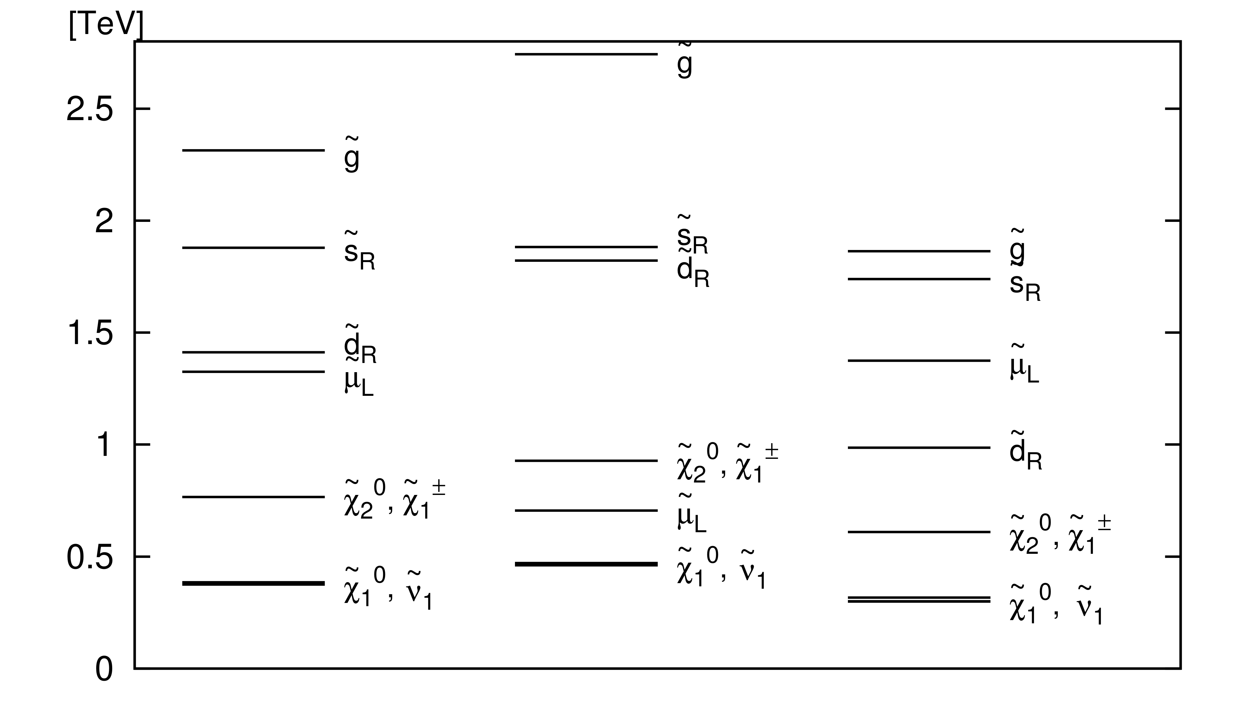
Figure 8: Examples of spectra characteristic of the $GFV_{23}$ Yukawa unification scenario.

All the points from our scan that demonstrate the Yukawa unification and satisfy the experimental constraints listed in Table 4 share the same characteristic pattern of the light part of the spectrum. Three examples are shown in Fig. 8. The Next-to-Lightest SUSY particle (NLSP) is the lightest sneutrino, while one charged slepton, neutralino $\tilde{{\chi}}^{0}_{2}$ and chargino $\tilde{{\chi}}^{\pm}_{1}$ are slightly heavier. The presence of light sleptons in the spectrum is very important as it leads to a characteristic 3-lepton signature at the LHC. The next particle on the mass ladder is the lightest down-type squark which is followed by the gluino. All the other coloured particles, the remaining sleptons and heavy Higgses are much heavier and effectively decoupled. Comparison of the production cross-sections reveals that the dominant production channels at the LHC would be direct $\tilde{d}_{1}\tilde{d}_{1}$, $\tilde{{\chi}}^{\pm}_{1}$$\tilde{{\chi}}^{0}_{2}$ and $\tilde{{\chi}}^{\pm}_{1}$$\tilde{{\chi}}^{\pm}_{1}$ production. The cross-section for gluino pair production is one order of magnitude lower, and practically all of the produced gluinos decay via $\tilde{g}\to\tilde{d}_{1}q$. Therefore, the Yukawa unification scenario is characterized by two distinct LHC signatures: 3 leptons plus missing energy (MET) signature for the electroweakino production, and 0 leptons, jets plus MET signature for the coloured particles production.

The strongest limit on the gluino mass comes from the ATLAS 0 lepton, 2-6 jets plus MET inclusive search [53] that provides a stringent 95% C.L. exclusion bound $m_{\tilde{g}}\gtrsim 1400\,\mathrm{GeV}$ for neutralino LSP lighter than $300\,\mathrm{GeV}$. The strongest bound on the lightest sbottom mass comes from the CMS 0 leptons, 2 jets and MET search [52], while in the electroweakino sector the most stringent experimental exclusion limits are obtained using the 3-lepton plus MET CMS search [54].

However, one needs to keep in mind that the bounds provided by the experimental collaborations are interpreted in the Simplified Model Scenarios (SMS) that make strong assumptions about the hierarchy of the spectrum and the decay branching ratios. Usually it is assumed that there is only one light SUSY particle apart from the neutralino LSP, and only one decay channel of the NLSP with the branching ratio set to 100% is considered. In a more general case, however, the presence of other light particles in the spectrum may alter the decay chain, and the assumption concerning the branching ratio may not hold either. In such a case, the exclusion limits for the SMS should be treated with care, and the actual limits are expected to be weaker.

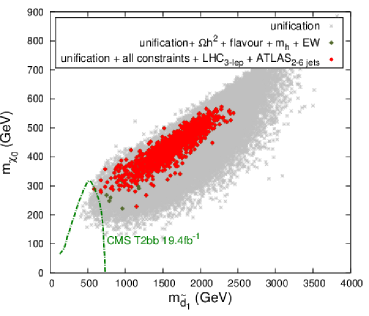
(a)

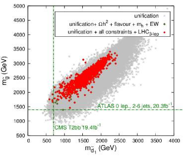
(b)

Figure 9: Scatter plot of the $GFV_{23}$ points in the planes ($m_{\tilde{d}_{1}}$, $m_{\tilde{\chi}^{0}_{1}}$) (a), and ($m_{\tilde{d}_{1}}$, $m_{\tilde{g}}$) (b). Gray stars: all the points that allow for the Yukawa coupling unification; dark green dots: points with good Yukawa coupling unification and all the constraints listed in Table 4 (except the LHC) satisfied at $3\sigma$; red diamonds: points additionally surviving the CMS 3-lepton search at $3\sigma$. Dashed lines correspond to 95% C.L. limits provided by other LHC SUSY searches discussed in the text.

In our analysis, we have used the experimental exclusion bound for the gluino mass [53] at face value because this search is inclusive and therefore tests any gluino-driven multijet signature, irrespectively of a particular decay chain. We have also decided to use a direct 95% C.L. limit from the CMS sbottom production search [52]. For the SMS T2bb, it reads $m_{\tilde{b}_{1}}\gtrsim 700\,\mathrm{GeV}$ for $m_{\tilde{\chi}^{0}_{1}}\simeq 150\,\mathrm{GeV}$, and $m_{\tilde{b}_{1}}\gtrsim 640\,\mathrm{GeV}$ for $m_{\tilde{\chi}^{0}_{1}}\simeq 250\,\mathrm{GeV}$. In our scenario, the sbottom decay corresponds exactly to the SMS T2bb, i.e. $\textrm{BR}(\tilde{b}\to b\tilde{\chi}^{0}_{1})=100\%$. We neglect here a possibility that the actual limit can be weakened due to significant mixing between the sbottoms and other down-type squarks, and we leave a detailed analysis of GFV effects in such a case for future studies. We will see, however, that this simplifying assumption is justified by the fact that the limits derived from Ref. [52] are not the dominant ones.

On the other hand, interpretation of the CMS 3-lepton search strongly depends on hierarchy in the considered spectrum, as well as on actual branching ratios for neutralino and chargino decays. Therefore, in order to correctly quantify the effect of this search in the $GFV_{23}$ scenario, we perform a full reinterpretation of the experimental analysis using the tools developed first in Ref. [25], and modified to recast the limits from SMS in Ref. [60]. For the purpose of the present study, we have updated the previously implemented [61] CMS 3-lepton search to include the full set of data with integrated luminosity of $19.5/\text{fb}$ [54].

In Fig. 9, we present a distribution of the model points in the ($m_{\tilde{d}_{1}}$, $m_{\tilde{\chi}^{0}_{1}}$) plane (a), and in the ($m_{\tilde{d}_{1}}$, $m_{\tilde{g}}$) plane (b). All the points for which the Yukawa coupling unification is possible are shown as gray stars, and those that additionally satisfy at $3\sigma$ the experimental constraints listed in Table 4 (except the LHC) as dark green dots. Finally, red diamonds depict the points that survive (at $3\sigma$) the CMS 3-lepton plus MET search. Dashed lines correspond to the 95% C.L. exclusion bounds from the CMS and ATLAS multijet searches described above, and should be interpreted as lower bounds on sbottom and gluino masses.

One can see that already at the LHC $\sqrt{s}=8\,\mathrm{TeV}$, the 3-lepton search provides a stronger constraint on the Yukawa unification scenario than the limits from Refs. [52] and [53], although even in this case only a small part of the parameter space is tested. The efficiency of the search is weakened with respect to the corresponding SMS, for which the interpretations are provided in the experimental analysis [54], since only one generation of light sleptons is present.

On the other hand, $GFV_{23}$ unification scenario has a chance to be fully tested during the second run of the LHC. Gluino masses up to $2.5\,\mathrm{TeV}$ will be probed at the LHC$\sqrt{s}=14\,\mathrm{TeV}$ with the luminosity of $300/\text{fb}$ [62] as long as neutralino LSP is lighter than $700\,\mathrm{GeV}$. The limits on the sbottom mass will be improved up to $1400\,\mathrm{GeV}$ for neutralinos lighter than $600\,\mathrm{GeV}$. Those limits can be further extended up to $3000\,\mathrm{GeV}$ and $1600\,\mathrm{GeV}$, respectively, for the final LHC luminosity of $3000/\text{fb}$.

4.2.4 Electroweak symmetry breaking

(a)

(b)

Figure 10: Histograms of points gathered by the $GFV_{23}$ scan as a function of $A^{d}_{33}/(Y^{d}_{33}\widetilde{m})$ at the scale $M_{SUSY}$: (a) all the points gathered by the scan; (b) enlarged vicinity of zero.

As mentioned in Sec. 3.3.1, the $GFV_{23}$ unification scenario allows large values of $A^{de}_{33}/M_{1/2}$ at $M_{\textrm{GUT}}$. This may lead to a global charge/colour breaking (CCB) minimum of the MSSM scalar potential. Indeed, large values of $A^{d}_{33}(M_{SUSY})$ make it easier to tune the Yukawa threshold corrections to the size required by bottom-tau and strange-muon Yukawa coupling unification, and most of our points that satisfy this unification condition correspond to $\frac{A^{d}_{33}}{Y^{d}_{33}\widetilde{m}}(M_{SUSY})\sim O(1)$, where $\widetilde{m}=\sqrt{(m_{\tilde{d}_{3}}^{2}+m_{\tilde{e}_{3}}^{2}+m_{H_{d}}^{2})/3}$. For some points however, this ratio is close to zero, as can be seen in the panel (a) of Fig. 10. Therefore, the $GFV_{23}$ scenario does not necessarily lead to a metastable vacuum, as the relevant factor $\frac{A^{d}_{33}}{Y^{d}_{33}\widetilde{m}}(M_{SUSY})$ can always be fitted to satisfy the coarse bound $\frac{A_{ii}}{Y_{ii}\widetilde{m}_{i}}<1$.

4.3 $\boldsymbol{GFV_{123}}$: unification of all three families

4.3.1 Lepton Flavour Violating observables

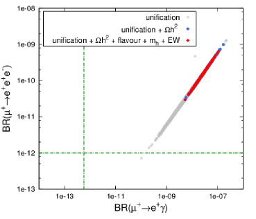
(a)

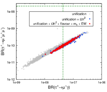
(b)

Figure 11: Scatter plot of the $GFV_{123}$ points in the planes ($\rm BR\left(\mu^{+}\to e^{+}\gamma\right)$, $\rm BR\left(\mu^{+}\to e^{+}e^{+}e^{-}\right)$) (a), and ($\rm BR\left(\tau^{\pm}\to e^{\pm}\gamma\right)$, $\rm BR\left(\tau^{\pm}\to e^{\pm}e^{+}e^{-}\right)$) (b). The colour code is the same as in Fig. 7.

In the $GFV_{123}$ scenario, the muon-electron conversion observables might be strongly enhanced, as they are influenced by large non-zero values of the parameters $m^{dl}_{12}$, $A^{de}_{12}$ and $A^{de}_{21}$, required by the Yukawa unification of the first family. In Fig. 11, we present distributions of model points in the planes ($\rm BR\left(\mu^{+}\to e^{+}\gamma\right)$, $\rm BR\left(\mu^{+}\to e^{+}e^{+}e^{-}\right)$) (a), and ($\rm BR\left(\tau^{\pm}\to e^{\pm}\gamma\right)$, $\rm BR\left(\tau^{\pm}\to e^{\pm}e^{+}e^{-}\right)$) (b). The colour code is the same as in Fig. 7. It is clear that the 90% C.L. upper bound on $\rm BR\left(\mu^{+}\to e^{+}\gamma\right)$ reported in Ref. [55] is violated in the $GFV_{123}$ scenario by about five orders of magnitude.

On the other hand, it is theoretically possible to evade this constraint while unifying the electron and down quark Yukawa couplings by raising the overall scale of the superpartner masses. However, such a scenario is difficult to test with our present numerical tools which assume $\mu_{\rm sp}=M_{Z}$ and henceforth are not reliable when $M_{\rm SUSY}$ is very large.

4.3.2 EW vacuum stability

There are also important non-decoupling effects of phenomenological importance that characterise the $GFV_{123}$ scenario, namely the vacuum (meta)stability problem. As discussed in Sec. 3, non-zero elements $A^{de}_{12/21}$ are required to achieve the Yukawa coupling unification for both the first and second families. However, off-diagonal entries of the trilinear couplings (as well as the diagonal ones) are strongly constrained by the requirement of EW vacuum stability. When the flavour-violating entries are too large, a CCB minimum may appear in the MSSM scalar potential, and it may become deeper than the standard EW one. The potential may also become unbounded from below (UFB) [63, 64, 65, 66, 67, 68]. An important feature of all such constraints is that, unlike the FCNC ones, they do not become weaker when the scale $M_{\rm SUSY}$ is increased.

In the down-squark sector, tree-level formulae for the CCB bounds are given by [68]

$$(v_{d}/\sqrt{2})A^{d}_{ij} \leq m^{d}_{k}[(m^{2}_{\tilde{q}})_{ii}+(m^{2}_{\tilde{d}})_{jj}+m_{H_{d}}^{2}+\mu^{2}]^{1/2},\quad k=\textrm{Max}(i,j).$$ (20)

The limits on $A^{e}_{ij}$ have an analogous form, up to replacing the matrix $m^{2}_{\tilde{d}}$ by $m^{2}_{\tilde{e}}$. Similarly, the UFB bounds read [68]

$$(v_{d}/\sqrt{2})A^{d}_{ij} \leq m^{d}_{k}[(m^{2}_{\tilde{q}})_{ii}+(m^{2}_{\tilde{d}})_{jj}+(m_{\tilde{l}}^{2})_{ii}+(m^{2}_{\tilde{e}})_{jj}]^{1/2},$$

$$(v_{d}/\sqrt{2})A^{e}_{ij} \leq \sqrt{3}m^{l}_{k},\quad k=\textrm{Max}(i,j).$$ (21)

In Fig. 12, we show to what extent the CCB and UFB limits are satisfied for the points that allow the Yukawa coupling unification and satisfy at $3\sigma$ all the experimental constraints listed in Table 4. Dashed line indicates the upper limit on the allowed size of the off-diagonal trilinear terms. One can see that the CCB stability bounds are violated by around an order of magnitude. The situation is even worse in the case of the UFB bounds where the size of the elements $A^{e}_{ij}$ are around four orders of magnitude larger than it is allowed by the stability constraint. It results from the fact that the UFB limit on $A^{e}_{ij}$ is of the order of the muon mass. Therefore, we conclude that the EW MSSM vacuum is not stable in the Yukawa unification scenario considered in our study.

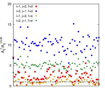
(a)

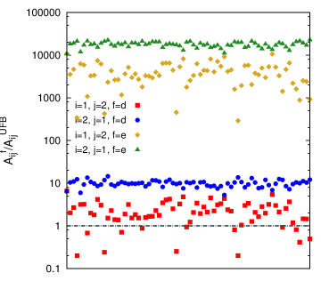
(b)

Figure 12: EW vacuum CCB (a) and UFB (b) stability bounds on the elements $A^{d}_{12/21}$ and $A^{e}_{12/21}$. Dashed line indicates the upper limit on the allowed size of the off-diagonal trilinear terms.

On the other hand, even if a CCB minimum appears, it does not imply that a considered model is not valid, as long as the standard EW vacuum lives longer than the age of the universe. Moreover, in such a case, the UFB bound becomes irrelevant because the probability of a tunnelling process along the CCB direction is much higher [69]. To derive metastability bounds, the bounce action for a given scalar potential should be calculated numerically, which is beyond the scope of our paper. To evaluate the impact of metastability on the validity of the unification scenario, we will use instead the results of the analysis performed in Ref. [69]. The derived metastability bounds do not depend on the Yukawa couplings, and therefore are in general much less stringent than the CCB ones. The effect is the strongest for the $A_{12/21}$ elements, in which case the CCB limit can be weakened by three to four orders of magnitude, depending on a particular choice of the model parameters. We can therefore conclude that the scenario considered in our study leads to an unstable, but a long-lived vacuum.

It should be stressed, though, that the tension between the Yukawa unification condition and the EW vacuum stability is less severe in our present scenario than in the case of Yukawa unification through large diagonal $A$-terms where the CCB bounds were violated by two orders of magnitude [10]. On the other hand, theoretical calculations of the stability conditions are still marred with many uncertainties. This leaves a possibility that future improvements might further reduce (or even eliminate) the tension between the vacuum stability and the Yukawa unification.

5 Conclusions

In this study, we provided evidence that $SU(5)$ boundary conditions for the Yukawa matrices at the GUT-scale can be satisfied within the renormalizable $R$-parity-conserving MSSM if a more general flavour structure of the soft SUSY-breaking sector is allowed. In particular, we found that a non-zero $(2,3)$ element of the down-type squark mass matrix helps to achieve an approximate Yukawa unification for the second family, as the SUSY threshold correction driven by this entry is proportional to the combination $(A^{d}_{33}-Y_{b}\mu\tan\beta$) that involves large third-generation couplings. Moreover, simultaneous unification of the Yukawa couplings for the second and first family additionally requires the elements $A_{12/21}^{de}$, $m^{dl}_{13}$ and $m^{dl}_{12}$ to assume non-zero values. The latter, however, leads to unacceptably large SUSY corrections to some Lepton Flavour Violating processes, in particular to $\mu\to e\gamma$ decay.

On the other hand, the scenario with Yukawa unification for the second and third family only, is consistent with a wide set of experimental measurements, including those from the FCNC processes, which are often raised as an argument against the GFV MSSM. The consistency holds even when theoretical uncertainties in determination of the flavour observables are reduced. We showed that a non-trivial flavour structure of the down-squark soft terms does not pose a threat for the quark-sector flavour observables for two reasons. First, the value of $\tan\beta$ required by both the Yukawa unification condition and the DM relic density measurement must stay in the range of $\tan\beta\in(10-30)$, so no large $\tan\beta$-enhancement occurs in supersymmetric loop corrections to rare $B$-meson decays. Secondly, squarks remain relatively heavy. This may suggest that the principle of Minimal Flavour Violation as a unique way to remain in agreement with the flavour observables is not always well motivated.

Another interesting feature of the $GFV_{23}$ unification scenario are the properties of dark matter. It turns out that the points with the Yukawa matrix unification are characterised by a neutralino LSP which is almost purely bino-like, and with the mass in the range of $200-600\,\mathrm{GeV}$. This, in turn, enforces a particular hierarchy of masses in the corresponding SUSY spectrum, with sneutrino NLSP and one light charged slepton. Spectra of this kind, that lead to a characteristic 3-lepton collider signature, have started to be tested in the direct SUSY searches at the LHC $\sqrt{s}=8\,\mathrm{TeV}$. In the upcoming LHC Run II, they are going to be tested in a complete manner.

Let us conclude with one more remark. The aim of our study was to check whether large GUT-scale threshold corrections to the Yukawa couplings or modifications of the Yukawa boundary conditions can be avoided in the $R$-parity conserving MSSM. We did not try, however, to construct a full and self-consistent model valid above the GUT-scale. For this reason some issues related to the minimal $SU(5)$ GUT, like the proton lifetime, remained unaddressed. On the other hand, ways of avoiding too fast proton decay in the framework of minimal $SU(5)$ have been proposed in the literature, for example by employing higher-dimensional operators [3]. It seems, therefore, feasible to combine two complementary approaches to the Yukawa coupling unification, the one using flavour-violating low-scale threshold corrections, and the one introducing higher-dimensional operators, to construct a correct $SU(5)$ UV-completion of the MSSM.

ACKNOWLEDGMENTS

We would like to thank Werner Porod for great help with issues related to SPheno. We also would like to thank Andreas Crivellin, Christophe Grojean, Gian Giudice, Mikołaj Misiak, Ulrich Nierste and Enrico Maria Sessolo for many useful comments and discussions. M.I. was supported in part by the Foundation for Polish Science International PhD Projects Programme co-financed by the EU European Regional Development Fund, by the Karlsruhe Institute of Technology, and by the National Science Centre (Poland) research project, decision DEC-2014/13/B/ST2/03969. K.K. was supported by the EU and MSHE Grant No. POIG.02.03.00-00-013/09. The use of the CIS computer cluster at the National Centre for Nuclear Research is gratefully acknowledged.

References

- [1] S. Dimopoulos and H. Georgi, Nucl. Phys. B 193 (1981) 150.
- [2] H. Georgi and C. Jarlskog, Phys. Lett. B 86 (1979) 297.
- [3] D. Emmanuel-Costa and S. Wiesenfeldt, Nucl. Phys. B 661 (2003) 62 [hep-ph/0302272].
- [4] S. Antusch and M. Spinrath, Phys. Rev. D 79 (2009) 095004 [arXiv:0902.4644 [hep-ph]].
- [5] S. Antusch, S. F. King and M. Spinrath, Phys. Rev. D 89 (2014) 055027 [arXiv:1311.0877 [hep-ph]].
- [6] W. Buchmuller and D. Wyler, Phys. Lett. B 121 (1983) 321.
- [7] L. J. Hall, V. A. Kostelecky and S. Raby, Nucl. Phys. B 267 (1986) 415.
- [8] J. L. Diaz-Cruz, H. Murayama and A. Pierce, Phys. Rev. D 65 (2002) 075011 [hep-ph/0012275].
- [9] T.Enkhbat, arXiv:0909.5597 [hep-ph].
- [10] M. Iskrzyński, Eur. Phys. J. C 75 (2015) 2, 51 [arXiv:1408.2165 [hep-ph]].
- [11] A. Crivellin, L. Hofer and J. Rosiek, JHEP 1107 (2011) 017 [arXiv:1103.4272 [hep-ph]].
- [12] A. Crivellin and U. Nierste, Phys. Rev. D 79 (2009) 035018 [arXiv:0810.1613 [hep-ph]].
- [13] A. Crivellin, Phys. Rev. D 83 (2011) 056001 [arXiv:1012.4840 [hep-ph]].
- [14] A. Crivellin and J. Girrbach, Phys. Rev. D 81 (2010) 076001 [arXiv:1002.0227 [hep-ph]].
- [15] J. Guasch and J. Sola, Nucl. Phys. B 562 (1999) 3 [hep-ph/9906268].
- [16] J. J. Cao, G. Eilam, M. Frank, K. Hikasa, G. L. Liu, I. Turan and J. M. Yang, Phys. Rev. D 75 (2007) 075021 [hep-ph/0702264].
- [17] S. Fichet, B. Herrmann and Y. Stoll, Phys. Lett. B 742 (2015) 69 [arXiv:1403.3397 [hep-ph]].
- [18] B. Herrmann, M. Klasen and Q. Le Boulc’h, Phys. Rev. D 84 (2011) 095007 [arXiv:1106.6229 [hep-ph]].
- [19] S. Heinemeyer, W. Hollik, F. Merz and S. Penaranda, Eur. Phys. J. C 37 (2004) 481 [hep-ph/0403228].
- [20] J. Cao, G. Eilam, K. i. Hikasa and J. M. Yang, Phys. Rev. D 74 (2006) 031701 [hep-ph/0604163].
- [21] M. Arana-Catania, S. Heinemeyer, M. J. Herrero and S. Penaranda, JHEP 1205 (2012) 015 [arXiv:1109.6232 [hep-ph]].
- [22] M. Arana-Catania, S. Heinemeyer and M. J. Herrero, Phys. Rev. D 90 (2014) 075003 [arXiv:1405.6960 [hep-ph]].
- [23] K. Kowalska, JHEP 1409 (2014) 139 [arXiv:1406.0710 [hep-ph]].
- [24] M. Arana-Catania, S. Heinemeyer and M. J. Herrero, Phys. Rev. D 88 (2013) 1, 015026 [arXiv:1304.2783 [hep-ph]].
- [25] A. Fowlie, M. Kazana, K. Kowalska, S. Munir, L. Roszkowski, E. M. Sessolo, S. Trojanowski and Y. L. S. Tsai, Phys. Rev. D 86 (2012) 075010 [arXiv:1206.0264 [hep-ph
- [26] F. Feroz, M. P. Hobson and M. Bridges, Mon. Not. Roy. Astron. Soc. 398 (2009) 1601 [arXiv:0809.3437 [astro-ph]].
- [27] W. Porod and F. Staub, Comput. Phys. Commun. 183 (2012) 2458 [arXiv:1104.1573 [hep-ph]].
- [28] K. A. Olive et al. [Particle Data Group Collaboration], Chin. Phys. C 38 (2014) 090001.
- [29] http://www.utfit.org/UTfit/ResultsSummer2014PostMoriondNP
- [30] A. Crivellin, J. Rosiek, P. H. Chankowski, A. Dedes, S. Jaeger and P. Tanedo, Comput. Phys. Commun. 184 (2013) 1004 [arXiv:1203.5023 [hep-ph]].
- [31] S. Aoki, Y. Aoki, C. Bernard, T. Blum, G. Colangelo, M. Della Morte, S. Dürr and A. X. El Khadra et al., Eur. Phys. J. C 74 (2014) 9, 2890 [arXiv:1310.8555 [hep-lat]].
- [32] Y. Amhis et al. [Heavy Flavor Averaging Group Collaboration], arXiv:1412.7515 [hep-ex].
- [33] M. Misiak, H. M. Asatrian, K. Bieri, M. Czakon, A. Czarnecki, T. Ewerth, A. Ferroglia, P. Gambino et al., Phys. Rev. Lett. 98 (2007) 022002 [hep-ph/0609232].
- [34] C. Bobeth, M. Gorbahn, T. Hermann, M. Misiak, E. Stamou and M. Steinhauser, Phys. Rev. Lett. 112 (2014) 101801 [arXiv:1311.0903 [hep-ph]].
- [35] J. Brod and M. Gorbahn, Phys. Rev. Lett. 108 (2012) 121801 [arXiv:1108.2036 [hep-ph]].
- [36] P. Gondolo, J. Edsjo, P. Ullio, L. Bergstrom, M. Schelke and E. A. Baltz, JCAP 0407 (2004) 008 [astro-ph/0406204].
- [37] T. Hahn, S. Heinemeyer, W. Hollik, H. Rzehak and G. Weiglein, Phys. Rev. Lett. 112 (2014) 141801 [arXiv:1312.4937 [hep-ph]].
- [38] M. Frank, T. Hahn, S. Heinemeyer, W. Hollik, H. Rzehak and G. Weiglein, JHEP 0702 (2007) 047 [hep-ph/0611326].
- [39] G. Degrassi, S. Heinemeyer, W. Hollik, P. Slavich and G. Weiglein, Eur. Phys. J. C 28 (2003) 133 [hep-ph/0212020].
- [40] S. Heinemeyer, W. Hollik and G. Weiglein, Comput. Phys. Commun. 124 (2000) 76 [hep-ph/9812320].
- [41] P. Bechtle, O. Brein, S. Heinemeyer, G. Weiglein and K. E. Williams, Comput. Phys. Commun. 181 (2010) 138 [arXiv:0811.4169 [hep-ph]].
- [42] P. Bechtle, O. Brein, S. Heinemeyer, G. Weiglein and K. E. Williams, Comput. Phys. Commun. 182 (2011) 2605 [arXiv:1102.1898 [hep-ph]].
- [43] P. Bechtle, O. Brein, S. Heinemeyer, O. Stål, T. Stefaniak, G. Weiglein and K. E. Williams, Eur. Phys. J. C 74 (2014) 2693 [arXiv:1311.0055 [hep-ph]].
- [44] P. Bechtle, S. Heinemeyer, O. Stål, T. Stefaniak and G. Weiglein, Eur. Phys. J. C 74 (2014) 2711 [arXiv:1305.1933 [hep-ph]].
- [45] D. S. Akerib et al. [LUX Collaboration], Phys. Rev. Lett. 112 (2014) 9, 091303 [arXiv:1310.8214 [astro-ph.CO]].
- [46] K. Cheung, Y. L. S. Tsai, P. Y. Tseng, T. C. Yuan and A. Zee, JCAP 1210 (2012) 042 [arXiv:1207.4930 [hep-ph]].
- [47] K. Kowalska, L. Roszkowski, E. M. Sessolo and S. Trojanowski, JHEP 1404 (2014) 166 [arXiv:1402.1328 [hep-ph]].
- [48] P. A. R. Ade et al. [Planck Collaboration], Astron. Astrophys. (2014) [arXiv:1303.5076 [astro-ph.CO]].
- [49] [CMS Collaboration], “Combination of standard model Higgs boson searches and measurements of the properties of the new boson with a mass near 125 GeV,” CMS-PAS-HIG-13-005.
- [50] V. Khachatryan et al. [CMS and LHCb Collaborations], Nature 522 (2015) 68 [arXiv:1411.4413 [hep-ex]].
- [51] C. A. Baker, D. D. Doyle, P. Geltenbort, K. Green, M. G. D. van der Grinten, P. G. Harris, P. Iaydjiev and S. N. Ivanov et al., Phys. Rev. Lett. 97 (2006) 131801 [hep-ex/0602020].
- [52] CMS Collaboration "Search for direct production of bottom squark pairs", CMS-PAS-SUS-13-018".
- [53] G. Aad et al. [ATLAS Collaboration], JHEP 1409 (2014) 176 [arXiv:1405.7875 [hep-ex]].
- [54] G. Aad et al. [ATLAS Collaboration], JHEP 1405 (2014) 071 [arXiv:1403.5294 [hep-ex]].
- [55] J. Adam et al. [MEG Collaboration], Phys. Rev. Lett. 110 (2013) 201801 [arXiv:1303.0754 [hep-ex]].
- [56] B. Aubert et al. [BaBar Collaboration], Phys. Rev. Lett. 104 (2010) 021802 [arXiv:0908.2381 [hep-ex]]
- [57] U. Bellgardt et al. [SINDRUM Collaboration], Nucl. Phys. B 299 (1988) 1.
- [58] K. Hayasaka, K. Inami, Y. Miyazaki, K. Arinstein, V. Aulchenko, T. Aushev, A. M. Bakich and A. Bay et al., Phys. Lett. B 687 (2010) 139 [arXiv:1001.3221 [hep-ex]].
- [59] E. Aprile [XENON1T Collaboration], Springer Proc. Phys. 148, 93 (2013) [arXiv:1206.6288 [astro-ph.IM]].
- [60] K. Kowalska and E. M. Sessolo, Phys. Rev. D 88, no. 7, 075001 (2013) [arXiv:1307.5790 [hep-ph]].
- [61] CMS Collaboration "Search for direct EWK production of SUSY particles in multilepton modes with 8TeV data", CMS-PAS-SUS-12-022".
- [62] ATLAS Collaboration "Search for Supersymmetry at the high luminosity LHC with the ATLAS experiment", ATL-PHYS-PUB-2014-010".
- [63] J. M. Frere, D. R. T. Jones and S. Raby, Nucl. Phys. B 222 (1983) 11.
- [64] L. Alvarez-Gaume, J. Polchinski and M. B. Wise, Nucl. Phys. B 221 (1983) 495.
- [65] J. P. Derendinger and C. A. Savoy, Nucl. Phys. B 237 (1984) 307.
- [66] C. Kounnas, A. B. Lahanas, D. V. Nanopoulos and M. Quiros, Nucl. Phys. B 236 (1984) 438
- [67] J. A. Casas, A. Lleyda and C. Muñoz, Nucl. Phys. B 471 (1996) 3 [hep-ph/9507294].
- [68] J. A. Casas and S. Dimopoulos, Phys. Lett. B 387 (1996) 107 [hep-ph/9606237].
- [69] J. h. Park, Phys. Rev. D 83 (2011) 055015 [arXiv:1011.4939 [hep-ph]].