SU-ITP-15/02
Holographic RG flows with nematic IR phases
Abstract
We construct zero-temperature geometries that interpolate between a Lifshitz fixed point in the UV and an IR phase that breaks spatial rotations but preserves translations. We work with a simple holographic model describing two massive gauge fields coupled to gravity and a neutral scalar. Our construction can be used to describe RG flows in non-relativistic, strongly coupled quantum systems with nematic order in the IR. In particular, when the dynamical critical exponent of the UV fixed point is and the IR scaling exponents are chosen appropriately, our model realizes holographically the scaling properties of the bosonic modes of the quadratic band crossing model.
1 Introduction
The past few years have seen increasing efforts to apply the tools of holography to probe condensed matter systems that are strongly coupled and typically poorly understood. The goal of this program is to provide qualitative as well as quantitative insights into the unconventional behavior of such systems, and in particular into their dynamical properties, which are challenging to probe using traditional techniques. As a result, we have seen the emergence of novel gravitational solutions – often encoding a number of broken symmetries – which mirror the rich structure of quantum phases familiar to the condensed matter community. Within this holographic program, geometries that break translations (and sometimes rotations) have received much attention recently. In fact, the breaking of translational invariance (as a way to incorporate lattice effects) has been recognized as a crucial ingredient for achieving a more realistic description of the conductive behavior of strongly correlated electron systems (see e.g. Hartnoll:2012rj ; Horowitz:2012ky ; Horowitz:2012gs ; Donos:2012js ; Vegh:2013sk ; Donos:2013eha ; Andrade:2013gsa ; Donos:2014yya ).
On the other hand, a gravitational description of the nematic phase, in which spatial rotations are the broken symmetries, has been largely unexplored. In particular, the question of how to obtain such phases in the infrared (IR) via renormalization group (RG) flow from a non-relativistic fixed point in the ultraviolet (UV) is still open. In this paper we would like to use the tools of holography to describe quantum systems which exhibit Lifshitz scaling in the UV, where they are rotationally and translationally invariant, and flow to a phase in the IR which breaks spatial rotations. If the latter phase has orientational order but no directional order (i.e., opposite directions are equivalent), it describes a system which is nematic. The order parameter for a nematic phase is a director, a symmetric traceless tensor. Nonetheless, a vector can also be used to describe a nematic, provided that its two possible directions and are identified. We will engineer the RG flows we are after by considering a simple phenomenological model in which gravity is coupled to two massive abelian gauge fields and a neutral scalar, with the latter settling to a constant at the endpoints of the flow. Our model has a global symmetry and therefore respects the rotational invariance crucial for nematics. However, upon developing a vacuum expectation value, the gauge field responsible for generating the spatial anisotropy in the IR can spontaneously break the symmetry111We are grateful to Sean Hartnoll for bringing this point to our attention. – a simple reflection of the fact that it is a vector and not a director. Thus, to ensure the absence of directional order, we will require to live on , where denotes the spatial directions of the QFT. In turn this will restrict the order parameter to live on , as desired for a nematic phase.
The concept of nematic ordering, which preserves the translational symmetry but breaks spontaneously the rotational symmetry down to two-fold, was originally developed in the study of finite-temperature thermal phase transitions in classical liquid crystals Chaikin1995 . Later it was discovered that quantum phases and quantum phase transitions with the same symmetry breaking pattern can also arise at zero temperature in strongly correlated electronic systems Kivelson1998 ; Fradkin2010 ; Xu2008 ; Hartnoll2014 . These quantum nematic phases have been observed in a wide range of materials and are proposed to be the key to understand important properties of systems including high temperature superconductors TRANQUADA1995 ; Ando2002 ; Kohsaka2007 ; Hinkov2008 ; Mesaros2011 , bilayer ruthenates Borzi2007 ; Raghu2009 , Fe-based superconductors Chuang2010 , two-dimensional electron gases Fradkin2000 , fractional quantum Hall systems Xia2011 , and doped manganites Tao2014 . Therefore, it is a valuable avenue to explore within the context of holography.
The construction of our paper applies generically to dimensional QFTs which exhibit the following Lifshitz symmetry in the UV,
| (1.1) |
with denoting the two spatial dimensions, while in the IR exhibit the scaling
| (1.2) |
In holography, Lifshitz fixed points can be geometrized by using a metric of the form
| (1.3) |
which is invariant under (1.1) as long as we scale , and reduces to when . Similarly, (1.2) can be realized geometrically by choosing
| (1.4) |
which is clearly invariant under (1.2), again provided that . Note that it preserves translations along the boundary directions , but breaks spatial rotations, unlike (1.3), due to the different scaling of the and coordinates. By appropriately choosing the potential for the scalar field in our model, we will construct RG flows connecting the UV fixed point (1.1) to IR phases described by (1.2). We will focus in particular on the values , , and , and construct a domain-wall solution which interpolates between (1.3) and (1.4).
While our setup is general enough to encompass flows to a variety of nematic phases, in this paper we would like to focus on applying it to a specific setting, namely that of the quadratic band crossing model. Indeed, as we will describe in detail in Section 2, the bosonic modes of the quadratic band crossing model exhibit interesting and quite non-trivial scalings depending on the energy scale of the physics that is being probed. At the UV fixed point, both bosonic and fermionic modes obey the Lifshitz symmetry (1.1), with the value of the dynamical critical exponent given by . In the IR, however, the (strong) interactions between the fermions and the bosons change the dynamics – and the scalings – of the latter. In particular, after integrating out the effects of the fermionic degrees of freedom, one finds that the bosonic modes scale according to (1.2), with the specific exponents given by and according to a one-loop self-energy correction. Thus, our holographic setup provides a first step towards describing the physics of the quadratic band crossing model, although we emphasize that it has broader applicability to IR nematic phases more generally. Finally, while in this paper we have used a massive vector field to break spatial rotations in the IR (and required it to live on to describe nematic order), we may also make a more general choice for the matter content of the bulk theory so that the order parameter is a director. We leave this to future work WorkInProgress .
The outline of the paper is as follows. Section 2 discusses the quadratic band crossing model and in particular the scaling of its bosonic modes. Section 3 contains our holographic model and the structure of perturbations about the IR and UV fixed points. In Section 4 we construct numerically a domain-wall solution interpolating between the two fixed points, focusing on , , and . We conclude in Section 5 with final remarks.
2 The quadratic band crossing model
For electrons in a solid, two different energy bands may share the same energy at certain momentum points, which are known as band crossing points. A famous example of this type is graphene, in which two bands touch each other at the and point of the Brillouin zone. Near these two band crossing points, the energies of the two bands scale linearly with the momentum, , where the momentum is measured from a band crossing point. There, the low-energy physics is described by the Dirac theory with dynamical critical exponent , and the band crossing point is referred to as a Dirac point. In addition to Dirac points, band crossing points with higher values of , e.g. , also exist. A 2+1 dimensional example can be found in bilayer graphene, a stack of two graphene layers, which has been experimentally realized and studied (see for example Refs. Nilsson2008 ; CastroNeto2009 ; Kotov2012 and references therein). Such a band crossing point is known as a quadratic band crossing point.
A quadratic band crossing point can be described by a two-component fermion spinor, . In dimensions, the action takes the following form
| (2.1) |
where and are two control parameters; and
| (2.2) |
are the dimensional -matrices. For band crossing points in a solid, and can take arbitrary values. Here we assume that the system preserves the charge conjugation symmetry (particle-hole) and is invariant under SO(2) space rotations. These two symmetries uniquely fix the control parameters and and fully determine the quadratic terms in the action
| (2.3) |
In the absence of interactions, it is easy to realize that this fermion has a quadratic dispersion relation , indicating that .222This system is a marginal case between a metal and an insulator. Although the fermionic modes are gapless in analogy to a metal, due to the zero fermion density there is no Fermi surface. As shown below, the absence of a Fermi surface greatly simplifies the RG analysis.
To describe interactions, we couple this fermion to bosonic modes. As shown in Ref. Sun2009 , to leading order this fermion can be coupled with four different bosonic modes , , , , and ,
| (2.4) |
where the ’s are the coupling constants. To ensure that the action is local, i.e. that there is no long-range interaction between fermions, we require the boson modes to be gapped. Without loss of generality, the gap can be set to unity
| (2.5) |
Here we ignore terms with derivatives in , because they are less relevant in the IR. For the action , dimension counting indicates that the system is scaling invariant with , i.e. , , , , and . The fact that implies that the couplings are marginal at tree level. To go beyond tree level, we first integrate out the bosons, which results in a four-Fermi interaction
| (2.6) |
with . A one-loop RG calculation has revealed that this interaction is marginally irrelevant in the IR if (attractive) and marginally relevant for (repulsive) Sun2009 .
Here we focus on the regime. In the UV, because the coupling scales down to zero, the scaling law is dictated by dimension counting and thus we find (for both bosons and fermions). In the IR, however, the interaction grows to infinity, and a phase transition will take place. Among the four bosonic modes, describes the charge fluctuations and the other three bosonic modes are order parameters for various symmetry breaking phases. If obtains a nonzero expectation value, the fermion gets a finite mass and becomes gapped, . This phase breaks spontaneously the time-reversal symmetry and is a topologically nontrivial quantum Hall insulator. The other two modes, and , form an representation of the rotational group . They give the order parameter of a nematic phase. If is nonzero, the rotational symmetry is broken spontaneously down to , i.e. only the rotation remains a symmetry operation. For , whether the time-reversal or the rotational symmetry will be broken in the IR is determined by microscopic details. Mean-field analysis for some lattice models indicates that the gapped topological insulator phase is favored at small , while strong coupling (large ) favors the nematic phase Sun2009 .
To better understand the nematic phase, without loss of generality we examine a case with and . It is easy to realize that here the massless Goldstone fluctuation is described by . To quadratic order, the action of the fermions becomes
| (2.7) |
This action contains two Weyl fermion points at momenta and . If we go to momentum space and expand the action near either of these two momentum points, a Weyl fermion action is obtained
| (2.8) |
where and are measured from either of the two Weyl points or , and the speed of light is determined by the order parameter . In summary, in the nematic phase the quadratic band crossing point at splits into two Weyl points at or , and the direction along which they split is determined by spontaneous symmetry breaking (for the case that we considered here, the splitting is along the axis). Because these two Weyl points are related by space inversion, they combine together and form a Dirac fermion with , in analogy to the Dirac fermion in graphene. In this nematic phase, the fermionic mode has at low energy and the reduction from in the UV to in the IR cures the instability.
Although the fermionic mode has , the low-energy boson modes in the nematic phase show different and interesting scaling relations. Here, we write down a phenomenological action for the Goldstone mode by including all terms allowed by symmetry. To leading order, the action takes the form
| (2.9) |
where the ’s are three control parameters. A key difference between this action and the one shown in Eq. (2.5) lies in the fact that here is gapless. This is because it is a Goldstone mode in the nematic phase. In the absence of the mass term, terms with derivatives become important and can no longer be ignored. Because is coupled to the fermionic modes , the fermions will introduce self-energy corrections and modify the dynamics of the mode as we integrate out the fermionic degrees of freedom. At low energies, we can treat the fermionic mode as a Dirac mode as shown above. Within this approximation, the one-loop self-energy correction is Pisarski1984 ; Appelquist1986 ; Gonzalez1994595 ; Kotov2012
| (2.10) |
and thus the effective theory for the mode is
| (2.11) |
In the IR, the self-energy correction dominates over the and terms in the original action and thus significantly changes the scaling behavior of the Goldstone mode. In the limit , , we have and , and thus the effective action becomes
| (2.12) |
Note that this action is scale invariant under
| (2.13) |
if we also scale the field accordingly.
It is worthwhile to emphasize that although the above scaling law is based on a one-loop self-energy calculation, the structure of the scaling relation may be more universal. For a Dirac system with symmetry, the self-energy correction must be invariant under rotations, i.e. Lorentz boost for and , and thus and are expected to have the same scaling behavior. Therefore, in the strong coupling limit, one may expect the scaling relation
| (2.14) |
although the values of and may deviate from the one-loop result. Next, we will examine how such scalings can be realized geometrically, using holography.
3 The holographic model
We are interested in building a model which will admit a zero-temperature flow from a non-relativistic UV fixed point described by (1.1) to an IR fixed point in which spatial rotations are broken, described by (1.2). Geometrically, this entails finding domain-wall solutions that connect (1.3) in the UV to (1.4) in the IR. Before introducing the particular model we will be working with, we would like to remind the reader that both (1.3) and (1.4) are exact solutions to the theory of a massive abelian gauge field coupled to gravity Kachru:2008yh ; Taylor:2008tg ,
| (3.1) |
where and are constant. In particular, the Lifshitz metric (1.3) can be supported by (3.1) when the gauge field is purely electric and is given by
| (3.2) |
with and . On the other hand, the IR metric (1.4) is an exact solution to (3.1) when the gauge field is oriented along the direction,
| (3.3) |
and the remaining parameters are related via and . Domain-wall solutions interpolating between different Lifshitz geometries, or between Lifshitz and AdS, have been constructed in a number of setups, typically involving gravity coupled to a massive gauge field – and sometimes a scalar – and their generalizations (see e.g. Kachru:2008yh ; Braviner:2011kz ; Liu:2012wf ; Kachru:2013voa ). As a concrete example, flows of this type can be obtained (see e.g. Liu:2012wf ) in simple phenomenological models of the form
| (3.4) |
in the presence of a background electric field .
Here, however, we are also interested in breaking spatial rotations in the IR, where we want the geometry to be described by (1.4), with different spatial directions exhibiting distinct scalings. To this end, a simple way to generalize the model (3.4) is to add a second massive gauge field . Thus, we take our working model to be of the form
| (3.5) |
with and , and the gauge fields and chosen so that
| (3.6) |
They will dominate the geometry in the UV and IR, respectively, where they will become and , generating a Lifshitz solution at high energies and one with broken spatial rotations in the opposite, low-energy regime. The scalar potential (or more precisely, the effective scalar potential ) will be chosen to drive the scalar field to constant values in the IR and UV, . Finally, we will be interested in solutions described by a diagonal metric,
| (3.7) |
where the two functions and will not generically be the same, in order to allow for the breaking of rotational symmetry at low energies.
At this stage we would like to elaborate on the role of the vector field responsible for the absence of spatial rotational symmetry in the IR. As we discussed briefly in the Introduction, a nematic phase has orientational order but no directional order – opposite directions in the plane are completely equivalent. As a consequence, its order parameter must respect the discrete symmetry (in particular, it must live on for the case of two spatial dimensions) and is generically described by a symmetric traceless tensor, i.e. a director. While a vector can still be used to describe nematic ordering, in order to do so its direction must be identified with the opposite one.
For our model, this means that the abelian gauge field must live on rather than simply . One possible way to realize the latter is by gauging the global symmetry of our theory (see e.g. Krauss:1988zc ; Banks:2010zn ). We expect that there shouldn’t be obstructions to doing so in the gravity theory, at least from an effective low-energy point of view. Whether this model can be UV completed is of course an important question which we don’t attempt to address here. In fact, it would be more desirable to choose the matter content of the model to reflect more directly the presence of a director, without resorting to using a vector. Nonetheless, the operation of gauging the global would then ensure that the overall sign of the gauge field is not physically observable, and that the order parameter of the IR phase is essentially . The trick of using the square of a vector to describe nematic order may work best in two spatial dimensions, which is the case we considered here, but fail or be more subtle in higher dimensions. This is because in two spatial dimensions a director and a vector have the same number of degrees of freedom, but this is no longer true in higher dimensions.
Finally, we should note that a spatial vector can be used as the order parameter for a ferromagnetic or a ferroelectric phase. In addition to rotational symmetry breaking, ferromagnetic order also breaks the time-reversal symmetry (the magnetization changes sign under time-reversal symmetry), while nematic or ferroelectric order is invariant under time-reversal. For our gravity setup, if we require the IR phase to preserve the time-reversal symmetry, the gauge field should be restricted to live on , which implies that our order parameter is in fact a director, instead of a vector, and thus the IR phase is nematic.
With these ingredients in place we will be able to engineer the flow we are after, in which the rotational symmetry is restored in the UV but the system is non-relativistic at every energy scale. While there should be alternative ways to build such systems, this particular model will allow us to work with simple ordinary differential equations, and to easily decouple some of the IR and UV perturbations from the rest, thus simplifying the analysis significantly. Also, at this stage our model is entirely phenomenological. Whether it can be embedded into string theory constructions is an interesting question, but is beyond the scope of our paper. We leave a more extensive analysis of how to engineer IR nematic phases to future work.
3.1 Domain-wall solutions
The equations of motion for our model (3.5) are given by
| (3.8) |
where primes denote derivatives with respect to the scalar field. Recall that our metric ansatz is (3.7) and we assumed that the gauge fields have the simple form given in (3.6).
In the IR the geometry is described by the following background solution,
| (3.9) |
provided that the scalar potential and coupling obey
| (3.10) | |||
| (3.11) |
Note that since vanishes to leading order in the IR geometry, the background equations of motion do not constrain the value of . For the purpose of describing the quadratic band crossing model we discussed in Section 2, we will eventually set and . However, for now we will keep these scalings arbitrary.
In the UV, on the other hand, the background is given by
| (3.12) |
supported by the following
| (3.13) | |||
| (3.14) |
It is now which is not constrained by the background equations of motion, again because vanishes to leading order in the UV. To satisfy the scaling of the quadratic band crossing model we will eventually need to take . For generality we will keep arbitrary for now. We will also assume that the UV (IR) fixed point is a local maximum (minimum) of the effective potential, i.e.
| (3.15) |
where . The scalar field will then roll from the maximum at to the minimum at . From the first equation in (3.1) it is evident that our domain-wall solutions will satisfy the null energy condition as long as and stay non-negative during the entire flow, as is true in the case that will be numerically studied in Section 4.
Next, we would like to study the response of the IR and UV geometries to linearized fluctuations, to ensure that we can find a well-behaved RG flow between the two fixed points.
3.1.1 IR perturbations
We start by examining the equation of motion for the scalar field,
| (3.16) |
Expanding the field in perturbations about its IR value and linearizing (3.16) we find that obeys
| (3.17) |
Notice that the scalar perturbation decouples from the metric and gauge field fluctuations and only when . Thus, to simplify the analysis and ensure decoupling we impose
| (3.18) |
where the second condition is needed to satisfy the background equations of motion. We emphasize that this restriction on is purely for convenience and is not required for a solution to exist. Finally, solving (3.17) we have
| (3.19) |
When the scaling exponents are given by and the two modes reduce to
| (3.20) |
To avoid turning on perturbations which are relevant about the IR fixed point, and which would therefore destabilize it, when constructing RG flow we will choose the mode which vanishes as and increases towards the boundary, as . The perturbation corresponding to the negative root is always divergent as the IR is approached, and thus needs to be turned off. To ensure that the other perturbation approaches zero as we need to impose
| (3.21) |
which coincides with the requirement that is a minimum of the effective scalar potential.
Next, we want to examine the behavior of the gauge field . Since it vanishes to leading order in the IR, its perturbation also decouples from the other fluctuations, and obeys the equation
| (3.22) |
with solution
| (3.23) |
When this reduces to
| (3.24) |
Thus, the scaling behavior of near the origin is controlled by the parameter , which is not specified by the background equations of motion. Again, the perturbation corresponding to the negative root is always divergent in the IR. The positive root corresponds to an irrelevant perturbation (growing towards the UV) provided that .
The remaining perturbations, involving the metric and the gauge field, are all coupled to each other. We will assume that they have an IR expansion of the form
| (3.25) | |||||
| (3.26) | |||||
| (3.27) | |||||
| (3.28) |
where we have left untouched.
Solving for the scaling exponent and the coefficients we find the following:
-
1.
a constant mode () with:
(3.29) -
2.
a mode which scales with and has
(3.30) This mode always diverges as the IR is approached (it is relevant) under the assumption that and are positive, and therefore needs to be discarded.
-
3.
a mode which scales with and has
(3.31) This mode is irrelevant provided that .
-
4.
a mode which scales as and has
(3.32) This mode is also always relevant (assuming ) and thus must be discarded.
Of these, the only mode which is irrelevant when the scaling exponents are and is the third one, which scales as and has:
| (3.33) |
Finally, counting all parameters we find 11 integration constants in the IR, 5 of which are associated with modes which are relevant and therefore need to be set to zero when constructing RG flow, and 3 of which are associated with a constant mode.
3.1.2 UV perturbations
We can now examine the structure of the perturbations in the UV, for a generic value of the dynamical critical exponent . Expanding the scalar equation of motion (3.16) to linear order in perturbations, with , we find that the fluctuation obeys
| (3.34) |
As before, the scalar field fluctuation decouples from the other ones provided that . Again, we will assume that this is the case in order to simplify the analysis, although it is by no means a necessary condition. In order to satisfy the background equations of motion we are then forced to take . Solving (3.34) we find the following modes,
| (3.35) |
When they reduce to:
| (3.36) |
In the UV, it is the fluctuation of the gauge field which decouples from the other modes, since the field vanishes to linear order. Letting we find
| (3.37) |
whose solutions are given by
| (3.38) |
Thus, the scaling of the perturbations can be controlled by tuning the value of , which is not determined by the background equations of motion.
The remaining fluctuations of the metric and the gauge field are all coupled together. Parametrizing them in the following way
| (3.39) | |||||
| (3.40) | |||||
| (3.41) | |||||
| (3.42) |
where we are leaving untouched. We find the following solutions:
-
1.
a constant mode () with
(3.43) -
2.
a mode which scales with and has
(3.44) -
3.
a mode which scales with and has
(3.45) -
4.
a mode which scales with and has
(3.46)
Note that these perturbations were already found in Ross:2009ar . As in the IR, we have 11 integration constants, 3 of which come from the constant mode.
The case , which is what we will focus on in Section 4 to describe the quadratic band crossing model, needs to be treated with some care Bertoldi:2009vn ; Ross:2009ar ; Cheng:2009df ; Holsheimer:2013ula . Note that when the third mode above becomes a constant, while the second and fourth modes both scale as . Indeed, for there are additional logarithmic modes which are not captured by our perturbation ansatz above and which can change the asymptotic form of the geometry. For a detailed discussion of these logarithmic modes without relying on linearizing the equations of motion, we refer the reader to Cheng:2009df . Here however we will work with linearized equations. The modes can then be taken into account by writing down the following ansatz for the perturbations:
| (3.47) | |||||
| (3.48) | |||||
| (3.49) | |||||
| (3.50) |
We then find the following solutions, in agreement with the analysis of Ross:2009ar ,
-
1.
with
(3.51) Since the leading logarithmic modes grow in the UV, we will impose as a boundary condition to ensure that the Lifshitz asymptotics are not changed Ross:2009ar . The role played by the leading log modes is actually quite rich. They were argued in Cheng:2009df to describe marginally relevant deformations of the theory. Finally, note that when this constant mode reduces to the one (3.43) we had already identified for general , which is a good consistency check.
- 2.
As before, we find that there are 11 integration constants in the UV. Here, we choose to turn off the leading log mode (i.e. setting in the solution above) and therefore lose one parameter. As we will see shortly, when constructing our domain-wall geometries numerically we will choose , , and to allow both modes of and in the UV. Thus, from the UV perspective, only 1 out of the 11 integration constants needs to be zero, and the remaining 10 parameters are free. Armed with the behavior of the IR and UV perturbations, we are now ready to construct the interpolating domain-wall solutions numerically.
4 Numerics
Since our main interest here is in applying our construction to the quadratic band crossing model, we will now focus on having in the UV and in the IR, although more general choices of scaling exponents are expected to yield similar results. To construct the domain-wall solutions we are after, we will choose the scalar potential and couplings , to be
| (4.1) |
As can be easily checked, these expressions satisfy the various requirements we imposed in Section 3. Note that we have taken the IR and UV values of the scalar field to be, respectively, and . The numerical solutions we present below were found using the shooting method. Moreover, the parameters in the model were tuned so that the UV Lifshitz fixed point would have no irrelevant modes, to make it easier to hit by shooting from the IR. Finally, the (irrelevant) IR modes where chosen to have the same scaling power, which we label by below, again to facilitate the numerical analysis.
For the numerical analysis we have found it convenient to use the following ansatz for the domain-wall solution,
| (4.2) |
The IR expansion we have used to set up the numerics, which is of course based on the perturbation analysis of Section 3, then takes the form
| (4.3) |
where the scaling exponent is given by
as can be read off by comparing with (3.33).
On the other hand, the UV expansion now takes the form
| (4.4) |
First, notice that the role of the leading log terms in the expressions for , and is simply to ensure that in the UV the solution is indeed the standard Lifshitz metric. These terms describe the background and should not be confused with the logarithmic modes we discussed in Section 3. The remaining perturbations of the metric and of , on the other hand, are either constant, or suppressed by , with the detailed structure of the latter perfectly consistent with (3.52). The marginally relevant log modes we discussed in Section 3 will not be turned on in the interpolating solution we have constructed, as will be apparent shortly. Finally, in the expansion of the scalar field we have .
Notice from these expansions that we have 6 parameters describing the IR, labelled by , and 10 parameter in the UV (having turned off the leading log mode) labelled by . The equation of motions in our model reduce to 1 first order ODE and 5 second order ODE, hence we need 11 integration constants to define a solution. We are then left with solutions parameterized by parameters. Furthermore, notice that the ansatz (4) has four unfixed scaling symmetries, described by:
| (4.5) | |||
| (4.6) | |||
| (4.7) | |||
| (4.8) |
After taking these into account, we are left with a one-parameter family of solutions333In the numerical analysis we have used a different metric ansatz, which is easier to work with, and have converted the result back to (4) by a coordinate transformation..
In Figures 1 and 2 we present a typical example of the interpolating solutions we have constructed numerically. In these solutions the breaking of (spatial) rotational symmetry is explicit, since . However, in our model we should also be able to realize spontaneous symmetry breaking, since we are working with a one-parameter family of solutions.
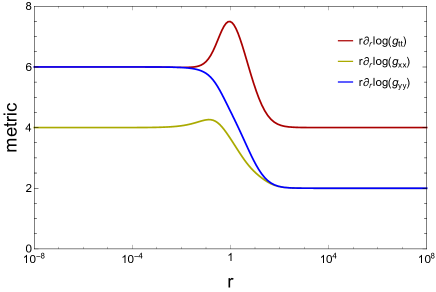
Figure 1 shows a logarithmic derivative plot444Logarithmic derivative plots are constructed so that any function scaling as will appear as a horizontal line with intercept at , making any scaling behavior readily apparent. of the radial dependence of the metric components , and . In the IR, which corresponds to , and both scale as , while scales as , as expected from the nematic solution (3.1) when . In the UV, as , it is the spatial components which scale in the same way (showing that spatial rotations are preserved), while , as expected from the Lifshitz geometry (3.1) when the critical exponent is . Thus, we see clearly the breaking of rotational symmetry as the solution approaches the IR of the geometry.
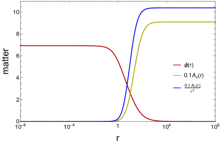
Figure 2 shows the radial dependence of the scalar field and of the two gauge fields (appropriately rescaled). We see that the scalar (denoted by the red line) interpolates between near to at the boundary, as desired. The gauge field (blue line) vanishes towards the IR in agreement with the perturbation analysis (4), and scales as in the UV, as expected from (4). Similarly, the spatial component (yellow line) scales as in the IR and approaches a constant in the UV, again in agreement with the IR and UV expansions (4) and (4).
In particular, from the UV behavior of it is apparent that in this background the leading log mode we discussed in Section 3 is not present. Although it would be interesting to find solutions for which it is turned on, it is beyond the scope of this analysis.
5 Conclusion
Our goal in this paper was to construct a simple gravitational model which would admit zero-temperature solutions interpolating between a UV Lifshitz fixed point and a nematic IR fixed point, in which spatial rotations are broken. Such a setup has broad applications to non-relativistic RG flows in quantum systems with nematic IR phases. For the specific scalings we have chosen, it can also be thought of as a first step towards describing holographically the behavior of the bosonic modes of the quadratic band crossing model, which obey the Lifshitz scaling (1.1) at high energies, and the nematic scaling (1.2) at lower energy scales. We emphasize that while in our numerical solutions we have chosen the scaling exponents to be , , and , our model (and the analytic results of Section 3) can be applied to generic values of these parameters.
The model that we have constructed couples gravity to two massive abelian gauge fields and a neutral scalar, with the latter controlling the gauge fields’ mass terms. Our setup should by no means be the only way to engineer RG flows of this type. However, it has the advantage of making the analysis particularly tractable, allowing us to work with ordinary differential equations and to decouple some of the IR and UV perturbations from the remaining ones. While at this stage the model is entirely phenomenological, we do not see any fundamental obstacles for being able to derive it from an appropriate supergravity truncation.
The value of the dynamical critical exponent we have chosen for the Lifshitz UV fixed point is interesting for several reasons. First, it corresponds to the case of the quadratic band crossing model which is currently well-studied and understood. Moreover, on the gravity side is somewhat special, since it is associated with the appearance of logarithmic modes which have been argued to describe marginally relevant deformations of the Lifshitz theory. Such modes affect the form of the geometry to leading order, thus modifying the Lifshitz asymptotics. In the particular domain-wall solution we have constructed the leading log modes are turned off, and therefore do not affect the UV behavior of the geometry. More generally, however, they are expected to be present, and it is interesting to ask what role they may play in the physics of the quadratic band crossing model, if any, and in nematic phases more broadly. We leave this question to future work.
Another interesting question is that of the stability of the IR nematic geometry. Since the spectrum of IR perturbations admits relevant modes, we expect that there should be additional geometries that the nematic solution may flow into, perhaps associated with the breaking of translational symmetry. Better understanding RG flow and RG stability would shed light on the interplay between nematic and smectic phases. Moreover, this would tie our construction to the recent efforts to probe the role of broken translations in determining the conductive behavior of e.g. strongly correlated electron systems. The competition between nematic and smectic IR phases and how it connects with the detailed behavior of the quadratic band crossing model is an avenue that we would like to explore in future work.
Acknowledgments
We are grateful to Shamit Kachru, Jim Liu, Chris Pope and Andy Royston for helpful discussions. We are especially thankful to Sean Hartnoll for insightful comments on the draft. S.C. is supported by the Cambridge-Mitchell Collaboration in Theoretical Cosmology, and the Mitchell Family Foundation. XD is supported by the National Science Foundation under grant PHY-0756174. JR is partially supported by the Mitchell Institute for Fundamental Physics and Astronomy. KS is supported by the National Science Foundation under grant PHY-1402971.
References
- (1) S. A. Hartnoll and D. M. Hofman, “Locally Critical Resistivities from Umklapp Scattering,” Phys. Rev. Lett. 108, 241601 (2012) [arXiv:1201.3917 [hep-th]].
- (2) G. T. Horowitz, J. E. Santos and D. Tong, “Optical Conductivity with Holographic Lattices,” JHEP 1207, 168 (2012) [arXiv:1204.0519 [hep-th]].
- (3) G. T. Horowitz, J. E. Santos and D. Tong, “Further Evidence for Lattice-Induced Scaling,” JHEP 1211, 102 (2012) [arXiv:1209.1098 [hep-th]].
- (4) A. Donos and S. A. Hartnoll, “Interaction-driven localization in holography,” Nature Phys. 9, 649 (2013) [arXiv:1212.2998].
- (5) D. Vegh, “Holography without translational symmetry,” arXiv:1301.0537 [hep-th].
- (6) A. Donos and J. P. Gauntlett, “Holographic Q-lattices,” JHEP 1404, 040 (2014) [arXiv:1311.3292 [hep-th]].
- (7) T. Andrade and B. Withers, “A simple holographic model of momentum relaxation,” JHEP 1405, 101 (2014) [arXiv:1311.5157 [hep-th]].
- (8) A. Donos and J. P. Gauntlett, “The thermoelectric properties of inhomogeneous holographic lattices,” arXiv:1409.6875 [hep-th].
- (9) P.M. Chaikin and TC Lubensky. Principles of condensed matter physics. Cambridge university press, 1995.
- (10) S. A. Kivelson, E. Fradkin, and V. J. Emery. Electronic liquid-crystal phases of a doped Mott insulator. Nature, 393:550, 1998.
- (11) Eduardo Fradkin, Steven A. Kivelson, Michael J. Lawler, James P. Eisenstein, and Andrew P. Mackenzie. Nematic fermi fluids in condensed matter physics. Annual Review of Condensed Matter Physics, 1(1):153–178, 2010.
- (12) Cenke Xu, Yang Qi, and Subir Sachdev. Experimental observables near a nematic quantum critical point in the pnictide and cuprate superconductors. Phys. Rev. B, 78:134507, 2008.
- (13) Sean A. Hartnoll, Raghu Mahajan, Matthias Punk, and Subir Sachdev. Transport near the Ising-nematic quantum critical point of metals in two dimensions. Phys. Rev. B, 89:155130, 2014.
- (14) J. M. Tranquada, B. J. Sternlieb, J. D. Axe, Y. Nakamura, and S. Uchida. Evidence for stripe correlations of spins and holes in copper oxide superconductors. Nature, 375:561, 1995.
- (15) Yoichi Ando, Kouji Segawa, Seiki Komiya, and A. Lavrov. Electrical resistivity anisotropy from self-organized one dimensionality in high-temperature superconductors. Phys. Rev. Lett., 88:137005, Mar 2002.
- (16) Y. Kohsaka, C. Taylor, K. Fujita, A. Schmidt, C. Lupien, T. Hanaguri, M. Azuma, M. Takano, H. Eisaki, H. Takagi, S. Uchida, and J. C. Davis. An intrinsic bond-centered electronic glass with unidirectional domains in underdoped cuprates. Science, 315(5817):1380–1385, 2007.
- (17) V. Hinkov, D. Haug, B. Fauqué, P. Bourges, Y. Sidis, A. Ivanov, C. Bernhard, C. T. Lin, and B. Keimer. Electronic liquid crystal state in the high-temperature superconductor YBCO(6.45). Science, 319(5863):597–600, 2008.
- (18) A. Mesaros, K. Fujita, H. Eisaki, S. Uchida, J. C. Davis, S. Sachdev, J. Zaanen, M. J. Lawler, and Eun-Ah Kim. Topological defects coupling smectic modulations to intra–unit-cell nematicity in cuprates. Science, 333(6041):426–430, 2011.
- (19) R. A. Borzi, S. A. Grigera, J. Farrell, R. S. Perry, S. J. S. Lister, S. L. Lee, D. A. Tennant, Y. Maeno, and A. P. Mackenzie. Formation of a nematic fluid at high fields in sr3ru2o7. Science, 315(5809):214–217, 2007.
- (20) S. Raghu, A. Paramekanti, E Kim, R. Borzi, S. Grigera, A. Mackenzie, and S. Kivelson. Microscopic theory of the nematic phase in . Phys. Rev. B, 79:214402, Jun 2009.
- (21) T.-M. Chuang, M. P. Allan, Jinho Lee, Yang Xie, Ni Ni, S. L. Bud’ko, G. S. Boebinger, P. C. Canfield, and J. C. Davis. Nematic electronic structure in the “parent ?state of the iron-based superconductor Ca(Fe1-xCox)2As2. Science, 327(5962):181–184, 2010.
- (22) Eduardo Fradkin, Steven Kivelson, Efstratios Manousakis, and Kwangsik Nho. Nematic phase of the two-dimensional electron gas in a magnetic field. Phys. Rev. Lett., 84:1982–1985, Feb 2000.
- (23) Jing Xia, J. P. Eisenstein, L. N. Pfeiffer, and K. W. West. Evidence for a fractionally quantized hall state with anisotropic longitudinal transport. Nature Physics, 7:845, 2011.
- (24) Jing Tao, Kai Sun, Weiguo Yin, S. J. Pennycook, J. M. Tranquada, and Yimei Zhu. Unveiling the microscopic origin of the electronic smectic-nematic phase transition in La1/3Ca2/3MnO3. arXiv:1403.7216, 2014.
- (25) S. Cremonini, X. Dong, J. Rong, K. Sun. Work in Progress.
- (26) Johan Nilsson, A. H. Castro Neto, F. Guinea, and N. M. R. Peres. Electronic properties of bilayer and multilayer graphene. Phys. Rev. B, 78(4):045405, 2008.
- (27) A. H. Castro Neto, F. Guinea, N. M. R. Peres, K. S. Novoselov, and A. K. Geim. The electronic properties of graphene. Rev. Mod. Phys., 81(1):109, 2009.
- (28) Valeri Kotov, Bruno Uchoa, Vitor Pereira, F. Guinea, and A. Castro Neto. Electron-electron interactions in graphene: Current status and perspectives. Rev. Mod. Phys., 84:1067–1125, Jul 2012.
- (29) Kai Sun, Hong Yao, Eduardo Fradkin, and Steven Kivelson. Topological insulators and nematic phases from spontaneous symmetry breaking in 2d fermi systems with a quadratic band crossing. Phys. Rev. Lett., 103:046811, Jul 2009.
- (30) Robert Pisarski. Chiral-symmetry breaking in three-dimensional electrodynamics. Phys. Rev. D, 29:2423–2426, May 1984.
- (31) Thomas Appelquist, Mark Bowick, Dimitra Karabali, and L. Wijewardhana. Spontaneous chiral-symmetry breaking in three-dimensional qed. Phys. Rev. D, 33:3704–3713, Jun 1986.
- (32) J. Gonzalez, F. Guinea, and M.A.H. Vozmediano. Non-fermi liquid behavior of electrons in the half-filled honeycomb lattice (a renormalization group approach). Nuclear Physics B, 424(3):595 – 618, 1994.
- (33) S. Kachru, X. Liu and M. Mulligan, “Gravity duals of Lifshitz-like fixed points,” Phys. Rev. D 78, 106005 (2008) [arXiv:0808.1725 [hep-th]].
- (34) M. Taylor, “Non-relativistic holography,” arXiv:0812.0530 [hep-th].
- (35) H. Braviner, R. Gregory and S. F. Ross, “Flows involving Lifshitz solutions,” Class. Quant. Grav. 28, 225028 (2011) [arXiv:1108.3067 [hep-th]].
- (36) J. T. Liu and Z. Zhao, “Holographic Lifshitz flows and the null energy condition,” arXiv:1206.1047 [hep-th].
- (37) S. Kachru, N. Kundu, A. Saha, R. Samanta and S. P. Trivedi, “Interpolating from Bianchi Attractors to Lifshitz and AdS Spacetimes,” JHEP 1403, 074 (2014) [arXiv:1310.5740 [hep-th]].
- (38) G. Bertoldi, B. A. Burrington and A. Peet, “Black Holes in asymptotically Lifshitz spacetimes with arbitrary critical exponent,” Phys. Rev. D 80, 126003 (2009) [arXiv:0905.3183 [hep-th]].
- (39) L. M. Krauss and F. Wilczek, “Discrete Gauge Symmetry in Continuum Theories,” Phys. Rev. Lett. 62, 1221 (1989).
- (40) T. Banks and N. Seiberg, “Symmetries and Strings in Field Theory and Gravity,” Phys. Rev. D 83, 084019 (2011) [arXiv:1011.5120 [hep-th]].
- (41) S. F. Ross and O. Saremi, “Holographic stress tensor for non-relativistic theories,” JHEP 0909, 009 (2009) [arXiv:0907.1846 [hep-th]].
- (42) M. C. N. Cheng, S. A. Hartnoll and C. A. Keeler, “Deformations of Lifshitz holography,” JHEP 1003, 062 (2010) [arXiv:0912.2784 [hep-th]].
- (43) K. Holsheimer, “On the Marginally Relevant Operator in Lifshitz Holography,” JHEP 1403, 084 (2014) [arXiv:1311.4539 [hep-th]].