Finite-Volume Spectra of the Lee-Yang Model

Abstract

We consider the non-unitary Lee-Yang minimal model ${\cal M}(2,5)$ in three different finite geometries: (i) on the interval with integrable boundary conditions labelled by the Kac labels $(r,s)=(1,1),(1,2)$, (ii) on the circle with periodic boundary conditions and (iii) on the periodic circle including an integrable purely transmitting defect. We apply $\varphi_{1,3}$ integrable perturbations on the boundary and on the defect and describe the flow of the spectrum. Adding a $\Phi_{1,3}$ integrable perturbation to move off-criticality in the bulk, we determine the finite size spectrum of the massive scattering theory in the three geometries via Thermodynamic Bethe Ansatz (TBA) equations. We derive these integral equations for all excitations by solving, in the continuum scaling limit, the TBA functional equations satisfied by the transfer matrices of the associated $A_{4}$ RSOS lattice model of Forrester and Baxter in Regime III. The excitations are classified in terms of $(m,n)$ systems. The excited state TBA equations agree with the previously conjectured equations in the boundary and periodic cases. In the defect case, new TBA equations confirm previously conjectured transmission factors.

1 Introduction

The determination of the full spectrum of a 1+1 dimensional Quantum Field Theory (QFT) in finite volume is a highly non-trivial and usually intractable task. Even the vacuum energy has a complicated volume dependence, which generally cannot be calculated exactly. For integrable theories the situation is better. The bootstrap approach provides exact expressions for the masses of the particles together with their scattering matrices. These infinite volume quantities can be used to determine an approximate spectrum via Bethe-Yang (BY) equations BY ; YangYang for large volumes. The BY finite size spectrum contains all polynomial corrections in the inverse powers of the volume but neglects exponentially small vacuum polarization effects. The vacuum polarization effects can be expressed in terms of the scattering matrix and, for the ground-state, they can be calculated exactly by the Thermodynamic Bethe Ansatz (TBA) method. The TBA method exploits the fact that for, large Euclidean time, the partition function is dominated by the contribution of the ground state. Exchanging the role of space and Euclidean time, the partition function only needs to be evaluated in the large volume limit, where Bethe-Yang equations are accurate. Calculating the partition function in the saddle point approximation, integral equations (TBA) can be derived for the saddle point particle densities (pseudo-energies). The solutions of these nonlinear TBA equations provides the ground-state energy Zam90 ; Zam91 .

The TBA method of exploiting the invariance properties of the partition function does not easily extend to excited states. Nevertheless, the exact ground-state TBA equations can be used to gain information about certain excited states Dorey under the assumption that these excited states and the ground-state are related by analytic continuation in a suitable variable. Carefully analysing the analytic behaviour of the TBA equations for complex volumes for these special excited states, TBA equations for zero momentum two particle states are obtained. The key difference, compared to the ground-state equation, is in the appearance of so called source terms, or equivalently, in choosing a different contour for integrations. Such a program using analytic continuation has not been successfully carried out to obtain TBA equations for the full excitation spectrum even for the simple non-unitary scaling Lee-Yang model LeeYang . Although, from the explicitly calculated cases, a natural conjecture for all exited states can be formulated. The Lee-Yang theory describes Fisher78 ; Cardy85 ; CardyMuss89 the closing, in the complex magnetic field plane, of the gap in the distribution of Lee-Yang zeros of the two-dimensional Ising model.

There is a more general and systematic way to obtain TBA integral equations for excited states based on functional relations PearK91 ; KlumP91 ; KlumP92 coming from Yang-Baxter integrable BaxBook lattice regularizations. These functional equations take the form of fusion, $T$- and $Y$-sytems. The $Y$-system involves the pseudo-energies and, at criticality, it describes the conformal spectra. It is universal in the sense that the same equations hold for all geometries and all excitations. Relevant physical solutions for the excitations are selected out by applying different asymptotic and analyticity properties to the $Y$-functions. Indeed, knowing this asymptotic and analytic information, the functional relations can be recast into TBA integral equations for the full excitation spectrum. This program has been successfully carried out to completion OPW97 for the tricritical Ising model ${\cal M}(4,5)$ with conformal boundary conditions. The lattice regularization approach is not limited to CFT but also extends to integrable QFTs. In PearN98 the ground-state TBA equations of the periodic $A$ and $D$ RSOS models were derived, while in PCAI ; PCAII the full spectrum of the tricritical Ising model was described on the interval. The integral equations for the spectrum of the sine-Gordon theory underwent a parallel development. The ground-state equation was derived in DdV and extended to some excited states in DdV2 ; FMQR .

The functional form of the $Y$-system reflects the integrable structure of the Conformal Field Theory (CFT). In principle, the $Y$-system can be derived BLZ directly in the continuum scaling limit. Within the lattice approach, it is obtained, in a more pedestrian way, by taking the continuum scaling limit of an integrable lattice regularization of the theory. A distinct advantage of the lattice approach is that it explicitly provides the asymptotic and analytic properties of the $Y$-functions, which otherwise need to be guessed. More specifically, the lattice approach provides the relevant asymptotic and analyticity properties and hence the complete classification of all excited states of the theory.

The Lee-Yang model ${\cal M}(2,5)$, perturbed by its only relevant spinless perturbation, is perhaps the simplest theory of a single massive particle and so is usually the first model studied to understand properties of massive theories. The scattering matrix is merely a simple CDD factor with a self-fusing pole

$$S(\theta)=\frac{\sinh\theta+i\sin\frac{\pi}{3}}{\sinh\theta-i\sin\frac{\pi}{3}}$$ (1)

The TBA equation for the model was derived by Zamolodchikov Zam90 ; Zam91

$$\epsilon(\theta)=mL\cosh\theta+s(\theta)-\int_{-\infty}^{\infty}\frac{d\theta^{{}^{\prime}}}{2\pi}\,\varphi(\theta-\theta^{{}^{\prime}})\log(1+e^{-\epsilon(\theta^{{}^{\prime}})})$$ (2)

where the kernel is related to the scattering matrix by $\varphi(\theta)=-i\partial_{\theta}\log S(\theta)$. For the ground state energy

$$E(L)=e(\theta)-m\int_{-\infty}^{\infty}\frac{d\theta}{2\pi}\,\cosh\theta\,\log(1+e^{-\epsilon(\theta)})$$ (3)

with vanishing source terms $s(\theta)=0$ and $e(\theta)=0$. Later, numerical investigation of the analytically continued TBA ground-state solution, for complex volumes, led Dorey to TBA equations for certain excited states with source terms

$$s(\theta)=\sum_{i}\log\frac{S(\theta-\theta_{i})}{S(\theta-\theta_{i}^{*})}$$ (4)

whose parameters are determined by the equations

$$\epsilon(\theta_{j})=i(2n_{j}+1)\pi$$ (5)

The contribution to the energy is $e(\theta)=-im\sum_{i}(\sinh\theta_{i}-\sinh\theta_{i}^{*})$. The $Y$-system Zam91

$$Y(\theta)=e^{\epsilon(\theta)},\qquad Y(\theta+\frac{i\pi}{3})Y(\theta-\frac{i\pi}{3})=1+Y(\theta)$$ (6)

of the Lee-Yang model has been recast BLZ as an integral equation by assuming the analytic properties of the $Y$-function thus providing a conjectured exact finite volume spectrum for periodic boundary conditions.

The Lee-Yang model has also been used as a prototypical example to extend integrability into other space-time geometries. The ground-state energy of the Lee-Yang model on the interval was derived in LMSS which, additionally to the $L\to 2L$ and $E\to 2E$ replacements, contained the left/right reflection factors $R_{\alpha/\beta}(\theta)$ in the source term

$$s(\theta)=-\log\Big{[}R_{\alpha}(\frac{i\pi}{2}+\theta)R_{\beta}(\frac{i\pi}{2}-\theta)\Big{]}$$ (7)

The analytic continuation method provided excited state TBA equations in DPTW ; DRTW with additional sources of the form (4), in which each $\theta_{i}$ is paired with a partner $-\theta_{i}$. Integrability also extends to include integrable defects of the Lee-Yang model. Indeed, the ground-state defect TBA equations were derived in BS with the source term being the logarithm of the transmission factor:

$$s(\theta)=-\log T_{+}(\frac{i\pi}{2}-\theta)$$ (8)

Perhaps surprisingly, the lattice regularization approach has not been systematically developed for the simple Lee-Yang theory and other non-unitary minimal models BPZ84 . Our aim is to fill this gap for the Lee-Yang theory. In the present paper we give a complete analysis of the finite volume spectrum of the Lee-Yang model in the various geometries using a lattice approach. It is expected that the methods developed here will apply to other non-unitary minimal models.

The paper is organized as follows: In Section 2, we introduce the Lee-Yang theory as the continuum scaling limit Huse84 ; Riggs89 of the $A_{4}$ RSOS lattice model of Forrester-Baxter ABF84 ; FB85 in Regime III with crossing parameter $\lambda=\frac{3\pi}{5}$. We set up commuting transfer matrices (i) with periodic boundary conditions, (ii) with an integrable defect (called a seam in the lattice terminology) and (iii) with two integrable boundaries. By properly normalizing the transfer matrices we show that they all satisfy the same universal functional relation in the form of a $Y$-system. The conformal spectra of these transfer matrices are analysed in Section 3. We investigate the analytic structure of the transfer matrix eigenvalues and classify all excited states. We do this first for the trigonometric theory whose scaling limit corresponds to the conformal Lee-Yang model. For the three geometries, we give detailed correspondences between paths, Virasoro descendants and patterns of zeros. The seam and boundaries admit a field which corresponds to the $\varphi_{1,3}$ perturbation. Appropriately varying this field implements FPR renormalization group flows connecting different conformal defect/boundary fixed points. We analyse the flow of the spectrum using the language of the paths, Virasoro descendants and zeros of the transfer matrix eigenvalues. Changing the trigonometric Boltzmann weights to suitable elliptic weights induces a massive $\Phi_{1,3}$ perturbation. We round out this section by also classifying the states of the massive theory. In Section 4, we combine the analytic information with the functional relations to derive integral TBA equations for the full finite volume spectrum in the various geometries in the critical case. The off-critical TBA equations are derived in Section 5. Finally, we conclude with some discussion in Section 6.

2 Lee-Yang Lattice Model and Transfer Matrices

The Lee-Yang lattice model is a Restricted Solid-On-Solid (RSOS) model ABF84 ; FB85 defined on a square lattice with heights $a=1,2,3,4$ restricted so that nearest neighbour heights differ by $\pm 1$. The heights thus live on the $A_{4}$ Dynkin diagram. It is convenient to regard the Lee-Yang model as a special case $L=4$ of the more general $A_{L}$ Forrester-Baxter FB85 models.

2.1 Lee-Yang lattice model as the $A_{4}$ RSOS model

The Boltzmann weights of the $A_{L}$ Forrester-Baxter FB85 models with heights $a=1,\ldots,L$ are

$$W\Big{(}\Big{.}\begin{array}[]{cc}a\pm 1&a\\ a&a\mp 1\end{array}\Big{|}u\Big{)} = \frac{s(\lambda-u)}{s(\lambda)}$$ (10)

$$W\Big{(}\Big{.}\begin{array}[]{cc}a&a\pm 1\\ a\mp 1&a\end{array}\Big{|}u\Big{)} = \frac{g_{a\mp 1}}{g_{a\pm 1}}\Big{(}\frac{s((a\pm 1)\lambda)}{s(a\lambda)}\Big{)}\,\frac{s(u)}{s(\lambda)}$$ (13)

$$W\Big{(}\Big{.}\begin{array}[]{cc}a&a\pm 1\\ a\pm 1&a\end{array}\Big{|}u\Big{)} = \frac{s(a\lambda\pm u)}{s(a\lambda)}.$$ (15)

Here $s(u)=\vartheta_{1}(u,q)$ is a standard elliptic theta function GR

$$\vartheta_{1}(u,q)=2q^{1/4}\sin u\prod_{n=1}^{\infty}(1-2q^{2n}\cos 2u+q^{4n})(1-q^{2n})$$ (16)

where $u$ is the spectral parameter and the square of the elliptic nome $t=q^{2}$ is a temperature-like variable corresponding to the $\Phi_{1,3}$ integrable bulk perturbation. The crossing parameter $\lambda$ is

$$\lambda=\frac{(m^{\prime}-m)\pi}{m^{\prime}}$$ (17)

where $m<m^{\prime}$, $m^{\prime}=L+1$ and $m,m^{\prime}$ are coprime integers. Integrability derives from the fact that these local face weights satisfy the Yang-Baxter equation. The gauge factors $g_{a}$ are arbitrary but we will take $g_{a}=1$. With this choice, the face weights are only symmetric under reflections about the NW-SE diagonal. Notice also that, in the non-unitary cases ($m^{\prime}\neq m+1$), some Boltzmann weights are negative. At criticality, $q=0$ and the function $s(u)$ can be taken to be $s(u)=\sin u$.

In the continuum scaling limit, the critical Forrester-Baxter models in Regime III

$$\mbox{Regime\leavevmode\nobreak\ III:}\qquad 0<u<\lambda,\qquad 0<q<1$$ (18)

are associated with the minimal models ${\cal M}(m,m^{\prime})$ with central charges

$$c=1-\frac{6(m-m^{\prime})^{2}}{mm^{\prime}}$$ (19)

In this paper, we only consider the Lee-Yang model

$${\cal M}(2,5):\qquad\lambda=\frac{3\pi}{5}$$ (20)

with central charge $c=-22/5$. The associated conformal Virasoro algebra admits two irreducible representations with conformal weights $h_{1,1}=h_{1,4}=0$, $h_{1,2}=h_{1,3}=-1/5$. It follows that the specific heat exponent $\alpha$ and correlation length exponent $\nu$ of the classical $d=2$ dimensional Lee-Yang model are given by the critical exponent scaling laws

$$h_{1,3}=\frac{1-\alpha}{2-\alpha},\qquad 2-\alpha=d\nu=2\nu,\qquad\alpha=\frac{7}{6},\qquad\nu=\frac{5}{12}$$ (21)

2.2 Transfer matrices and functional relations

In this section, we construct transfer matrices $T(u)$ from the local face weights. Since the local face weights satisfy the Yang-Baxter equations, the transfer matrices form commuting families $[T(u),T(v)]=0$ from which integrable one-dimensional quantum chains can be derived BEPR in the Hamiltonian limit. These transfer matrices satisfy the functional relations

$$\mbox{\boldmath$T$}(u)\mbox{\boldmath$T$}(u+\lambda)=\mathbbm{1}+\mbox{\boldmath$Y$}\mbox{\boldmath$T$}(u+3\lambda)$$ (22)

where $Y$ is the $\mathbb{Z}_{2}$ height reversal matrix. Apart from the change in the value of the crossing parameter $\lambda$ from $\frac{\pi}{5}$ to $\frac{3\pi}{5}$, this is the same functional equation BaxP82 ; BaxP83 that holds for the tricritical hard square and hard hexagon models Bax80 ; BaxBook . This simple change in the crossing parameter, however, drastically changes the relevant analyticity properties of the model.

The conformal spectra $E_{n}$ of the Lee-Yang model in different geometries can be extracted from the logarithm of the transfer matrix eigenvalue via finite-size corrections BCN . For periodic systems (with or without a seam) or in the presence of a boundary, the finite-size corrections are given respectively by

$$\mbox{}-\!\log T(u) =Nf_{\text{\tiny bulk}}(u)+f_{\text{\tiny s}}(u,\xi)+\frac{2\pi}{N}\big{[}(E_{n}\!+\!\bar{E}_{n})\sin\vartheta+i(E_{n}\!-\!\bar{E}_{n})\cos\vartheta\big{]}+o\big{(}\frac{1}{N}\big{)}$$ (23)

$$\mbox{}-\!\log T(u) =2Nf_{\text{\tiny bulk}}(u)+f_{\text{\tiny b}}(u,\xi)+\frac{2\pi}{N}\,E_{n}\sin\vartheta+o\big{(}\frac{1}{N}\big{)}$$ (24)

where $N$ is the number of columns, $\vartheta=\tfrac{5u}{3}$ is the anisotropy angle, $f_{\text{\tiny bulk}}(u)$ is the bulk free energy per column and $f_{\text{\tiny s/b}}(u)$ is the seam/boundary free energy. There is no seam free energy for periodic boundary conditions without a seam. The bulk, seam and boundary free energies can be calculated Stroganov ; Bax82Inv ; OBrienP97 by the inversion relation method. In the following, we derive the functional relations in the different geometries.

2.2.1 Periodic boundary condition

The entries of the transfer matrices $\mbox{\boldmath$T$}_{1,2}$ with periodic boundary conditions are defined on a lattice with $N$ columns with $N$ even by

$$\mbox{\boldmath$T$}_{j}(u)_{\mbox{\scriptsize\boldmath$a$}}^{\mbox{\scriptsize\boldmath$b$}}=W_{j}\Big{(}\Big{.}\begin{array}[]{cc}b_{1}&b_{2}\\ a_{1}&a_{2}\end{array}\Big{|}u\Big{)}W_{j}\Big{(}\Big{.}\begin{array}[]{cc}b_{2}&b_{3}\\ a_{2}&a_{3}\end{array}\Big{|}u\Big{)}\dots W_{j}\Big{(}\Big{.}\begin{array}[]{cc}b_{N-1}&b_{N}\\ a_{N-1}&a_{N}\end{array}\Big{|}u\Big{)}W_{j}\Big{(}\Big{.}\begin{array}[]{cc}b_{N}&b_{1}\\ a_{N}&a_{1}\end{array}\Big{|}u\Big{)}$$ (25)

For $j=1$, we take the fundamental weight $W_{1}=W$. For $j=2$, the transfer matrix $T_{2}(u)$ coincides with the $1\times 2$ fused face weight

$$W_{2}\Big{(}\Big{.}\begin{array}[]{cc}d&c\\ a&b\end{array}\Big{|}u\Big{)}=\frac{s(\lambda)}{s(u)}\sum_{e}W\Big{(}\Big{.}\begin{array}[]{cc}e&f\\ a&b\end{array}\Big{|}u\Big{)}W\Big{(}\Big{.}\begin{array}[]{cc}d&c\\ e&f\end{array}\Big{|}u\!+\!\lambda\Big{)}$$ (26)

In the gauge $g_{a}=(-1)^{a/2}$, these weights are independent of $f$ and are non-vanishing only when $|a-d|=0,2$ and $a+d=4,6$. The transfer matrices $\mbox{\boldmath$T$}_{1,2}$ satisfy a simple fusion functional equation

$$\mbox{\boldmath$T$}_{1}(u)\mbox{\boldmath$T$}_{1}(u+\lambda)=\Big{(}\frac{s(u+\lambda)s(\lambda-u)}{s^{2}(\lambda)}\Big{)}^{N}\mathbbm{1}+\Big{(}\frac{s(u)}{s(\lambda)}\Big{)}^{N}\mbox{\boldmath$T$}_{2}(u)$$ (27)

The Lee-Yang theory is the simplest of the non-unitary RSOS models. In this case, the fused weights $W_{2}$ are trivially related to $W_{1}$ modulo some $u$-independent gauge factors

$$W_{2}\Big{(}\Big{.}\begin{array}[]{cc}d&c\\ a&b\end{array}\Big{|}u\Big{)}=\frac{G_{a}G_{c}}{G_{b}G_{d}}\,W\Big{(}\Big{.}\begin{array}[]{cc}d&c\\ 5-a&5-b\end{array}\Big{|}u+3\lambda\Big{)}$$ (28)

The gauge factors $G_{a}$ do not contribute to the transfer matrix so that $\mbox{\boldmath$T$}_{1}(u)=\mbox{\boldmath$Y$}\mbox{\boldmath$T$}_{2}(u)=\mbox{\boldmath$T$}_{2}(u)\mbox{\boldmath$Y$}$. If we normalize the transfer matrix

$$\mbox{\boldmath$T$}(u)=\Big{(}\frac{s(\lambda)s(u+2\lambda)}{s(u+\lambda)s(u+3\lambda)}\Big{)}^{N}\mbox{\boldmath$T$}_{1}(u)$$ (29)

then $\mbox{\boldmath$T$}(u)$ satisfies the functional relation

$$\mbox{\boldmath$T$}(u)\mbox{\boldmath$T$}(u+\lambda)=\mathbbm{1}+\mbox{\boldmath$Y$}\mbox{\boldmath$T$}(u\!+\!3\lambda)$$ (30)

The height reversal matrix $Y$ commutes with $T$ so it can diagonalized in the same basis. Since $\mbox{\boldmath$Y$}^{2}=1$ the eigenvalues are $Y=\pm 1$. Restricting our analysis to the $Y=+1$ eigenspace, the eigenvalues $t(u)$ of the transfer matrix $\mbox{\boldmath$t$}(u)$ satisfy the functional equation

$$t(u)t(u+\lambda)=1+t(u+3\lambda)$$ (31)

The eigenvalues of the transfer matrix also satisfies the crossing relation and periodicity

$$t(\lambda-u)=t(u),\qquad t(u+\pi)=t(u)$$ (32)

2.2.2 Periodic boundary condition with a seam

The entries of the transfer matrices $\mbox{\boldmath$T$}_{1,2}$ for periodic boundary condition and a simple single-defect seam CMOP with parameter $\xi$ on a lattice of $N$ columns with $N$ even are

$$\mbox{\boldmath$T$}_{j}^{s}(u)_{\mbox{\scriptsize\boldmath$a$}}^{\mbox{\scriptsize\boldmath$b$}}=W_{j}\Big{(}\Big{.}\begin{array}[]{cc}b_{1}&b_{2}\\ a_{1}&a_{2}\end{array}\Big{|}u\!+\!\xi\Big{)}W_{j}\Big{(}\Big{.}\begin{array}[]{cc}b_{2}&b_{3}\\ a_{2}&a_{3}\end{array}\Big{|}u\Big{)}\dots W_{j}\Big{(}\Big{.}\begin{array}[]{cc}b_{2N-1}&b_{2N}\\ a_{2N-1}&a_{2N}\end{array}\Big{|}u\Big{)}W_{j}\Big{(}\Big{.}\begin{array}[]{cc}b_{2N}&b_{1}\\ a_{2N}&a_{1}\end{array}\Big{|}u\Big{)}$$ (33)

where the superscript $s$ refers to the seam. The parameter $\xi$ is arbitrary and can be complex. These transfer matrices satisfy the functional equation

$$\mbox{\boldmath$T$}_{1}^{s}(u)\mbox{\boldmath$T$}_{1}^{s}(u\!+\!\lambda)=\frac{s(u\!+\!\lambda\!+\!\xi)s(\lambda\!-\!u\!-\!\xi)}{s^{2}(\lambda)}\Big{(}\frac{s(u\!+\!\lambda)s(\lambda\!-\!u)}{s^{2}(\lambda)}\Big{)}^{N-1}\mathbbm{1}+\frac{s(u\!+\!\xi)}{s(\lambda)}\Big{(}\frac{s(u)}{s(\lambda)}\Big{)}^{N-1}\mbox{\boldmath$T$}_{2}^{s}(u)$$ (34)

If we restrict to the $Y=+1$ eigenspace and normalize the transfer matrix

$$\mbox{\boldmath$T$}^{s}(u)=\frac{s(\lambda)s(u+2\lambda+\xi)}{s(u+\lambda+\xi)s(u+3\lambda+\xi)}\Big{(}\frac{s(\lambda)s(u+2\lambda)}{s(u+\lambda)s(u+3\lambda)}\Big{)}^{N-1}T_{1}^{s}(u)$$ (35)

then the eigenvalues $t(u)$ satisfy the functional relation (31).

We note that the $\xi\to 0$ limit reproduces the periodic result corresponding to the $(r,s)=(1,1)$ identity seam. To produce the $(r,s)=(1,2)$ conformal seam, we renormalize the critical seam weights and take the braid limit $\xi\to i\infty$

$$W^{s}\Big{(}\Big{.}\begin{array}[]{cc}d&c\\ a&b\end{array}\Big{)}=\lim_{\xi\to i\infty}\frac{s(\lambda)}{s(\frac{\lambda}{2}\!-\!u\!-\!\xi)}\,W\Big{(}\Big{.}\begin{array}[]{cc}d&c\\ a&b\end{array}\Big{|}u+\xi\Big{)}=e^{i\frac{\lambda}{2}}\,\delta(a,c)-e^{-i\frac{\lambda}{2}}\,\frac{g_{a}}{g_{c}}\frac{s(c\lambda)}{s(b\lambda)}\,\delta(b,d)$$ (36)

2.2.3 Boundary case

To ensure integrability of the Lee-Yang lattice model in the presence of a boundary BPO96 we need commuting double row transfer matrices and triangle boundary weights which satisfy the boundary Yang-Baxter equations. The conformal boundary conditions are labelled by the Kac labels $(r,s)=(1,s)$ with $s=1,2$. These conformal boundary conditions can be realized in terms of integrable boundary conditions in different ways. For $(r,s)=(1,1)$, the non-zero left and right triangle weights are given by

$$K_{L}\Big{(}\Big{.}\begin{array}[]{c}1\\ 1\end{array}2\Big{|}u\Big{)}=\frac{s(2\lambda)}{s(\lambda)},\qquad K_{R}\Big{(}\Big{.}2\begin{array}[]{c}1\\ 1\end{array}\Big{|}u\Big{)}=1$$ (41)

Another integrable boundary can be constructed BP00 by acting with a seam on the $(1,1)$ integrable boundary. The non-zero right boundary weights are

$$K_{R}\Big{(}\Big{.}a\begin{array}[]{c}2\\ 2\end{array}\Big{|}u,\xi\Big{)} = W\Big{(}\Big{.}\begin{array}[]{cc}a&2\\ 2&1\end{array}\Big{|}u\!+\!\xi\Big{)}W\Big{(}\Big{.}\begin{array}[]{cc}2&1\\ a&2\end{array}\Big{|}\lambda\!-\!u\!+\!\xi\Big{)}K_{R}\Big{(}\Big{.}2\begin{array}[]{c}1\\ 1\end{array}\Big{|}u\Big{)}$$

$$= \frac{s(u+\xi+(2\!-\!a)\lambda)s(u-\xi+(2\!-\!a)\lambda)}{s(\lambda)s(2\lambda)},\quad a=1,3$$

Generically, for RSOS models in the continuum scaling limit with $\xi$ real, this integrable boundary converges to either the $(r,s)=(1,1)$ or $(2,1)$ conformal boundary condition depending on the real value of $\xi$. However, since $(r,s)=(2,1)$ does not exist for the Lee-Yang theory, this boundary condition converges in the continuum scaling limit to the $(1,1)$ conformal boundary condition for all real values of $\xi$. To obtain the $(r,s)=(1,2)$ boundary condition, we need to renormalize these boundary weights to obtain a nontrivial braid limit as $\xi\to i\infty$. The explicit $(r,s)=(1,2)$ non-zero right boundary weights in this limit are

$$K_{R}\Big{(}\Big{.}1\begin{array}[]{c}2\\ 2\end{array}\Big{|}u\Big{)}=K_{R}\Big{(}\Big{.}3\begin{array}[]{c}2\\ 2\end{array}\Big{|}u\Big{)}=1$$ (55)

In this way, varying $\mathop{\rm Im}\xi$ between $0$ and $\infty$ in (2.2.3) interpolates between the $(1,1)$ and $(1,2)$ conformal boundary conditions. Integrability, in the presence of these boundaries, derives from the fact that these boundary weights satisfy the left and right boundary Yang-Baxter equations, respectively. In the following, we fix the left boundary weight to be $(1,1)$ and take the right boundary weight to be either $(1,1)$ or $(1,2)$.

The face and triangle boundary weights are used to construct BPO96 a family of commuting double row transfer matrices $\mbox{\boldmath$T$}^{b}(u)$, where $b$ refers to the boundary case. For a lattice of width $N$, the entries of the transfer matrix $\mbox{\boldmath$T$}^{b}(u)$ are

$$\mbox{\boldmath$T$}_{1}^{b}(u)_{\mbox{\scriptsize\boldmath$a$}}^{\mbox{\scriptsize\boldmath$b$}} = \sum_{c_{1},\dots,c_{N}}K_{L}\Big{(}\Big{.}\begin{array}[]{c}1\\ 1\end{array}2\Big{|}\lambda\!-\!u\Big{)}W\Big{(}\Big{.}\begin{array}[]{cc}1&b_{1}\\ 2&c_{1}\end{array}\Big{|}\lambda\!-\!u\Big{)}W\Big{(}\Big{.}\begin{array}[]{cc}b_{1}&b_{2}\\ c_{1}&c_{2}\end{array}\Big{|}\lambda\!-\!u\Big{)}\dots W\Big{(}\Big{.}\begin{array}[]{cc}b_{N-1}&s\\ c_{N-1}&c_{N}\end{array}\Big{|}\lambda\!-\!u\Big{)}$$ (73)

$$\mbox{}\times W\Big{(}\Big{.}\begin{array}[]{cc}2&c_{1}\\ 1&a_{1}\end{array}\Big{|}u\Big{)}W\Big{(}\Big{.}\begin{array}[]{cc}c_{1}&c_{2}\\ a_{1}&a_{2}\end{array}\Big{|}u\Big{)}\dots W\Big{(}\Big{.}\begin{array}[]{cc}c_{N-1}&c_{N}\\ a_{N-1}&s\end{array}\Big{|}u\Big{)}K_{R}\Big{(}\Big{.}c_{N}\begin{array}[]{c}s\\ s\end{array}\Big{|}u\Big{)}\quad\qquad$$

This transfer matrix is positive definite and satisfies crossing symmetry $\mbox{\boldmath$T$}_{1}^{b}(u)=\mbox{\boldmath$T$}_{1}^{b}(\lambda-u)$. Although $\mbox{\boldmath$T$}_{1}^{a}(u)$ is not symmetric or normal, this one-parameter family of transfer matrices can be diagonalized because $\tilde{\mbox{\boldmath$T$}}_{1}^{b}(u)=\mbox{\boldmath$G$}\mbox{\boldmath$T$}_{1}^{b}(u)=\tilde{\mbox{\boldmath$T$}}_{1}^{b}(u)^{T}$ is symmetric where the diagonal gauge matrix $G$ is given by

$$\mbox{\boldmath$G$}_{\mbox{\scriptsize\boldmath$a$}}^{\mbox{\scriptsize\boldmath$b$}}=\prod_{j=1}^{N-1}G(a_{j},a_{j+1})\,\delta(a_{j},b_{j}) G(a,b)=\begin{cases}s(\lambda)/s(2\lambda),&b=1,4\\ 1,&\mbox{otherwise}\end{cases}$$ with (74)

It is convenient to define the normalized transfer matrix

$$\mbox{\boldmath$T$}^{b}(u)=S_{b}(u)\,\frac{s^{2}(2u-\lambda)}{s(2u+\lambda)s(2u-3\lambda)}\Bigl{(}\frac{s(\lambda)s(u+2\lambda)}{s(u+\lambda)s(u+3\lambda)}\Bigr{)}^{2N}\mbox{\boldmath$T$}(u)$$ (75)

with

$$S_{s}(u) = \begin{cases}1,&s=1\\ \frac{s^{2}(\lambda)}{s(u+\xi+\lambda)s(u-\xi+\lambda)s(u+\xi-\lambda)s(u-\xi-\lambda)}&s=2\end{cases}$$ (76)

It can then be shown BPO96 that, in the $Y=+1$ eigenspace, the eigenvalue $t(u)$ of the normalized transfer matrix $\mbox{\boldmath$T$}(u)=\mbox{\boldmath$T$}_{1}(u)$ satisfies the universal $Y$-system (31) independent of the boundary conditions labelled by $s=1,2$.

3 Classification of States

In this section, we exhaustively classify the states of the Lee-Yang theory. We start with the critical case and describe correspondences between the conformal basis FNO , the distribution of complex zeros of the transfer matrix eigenvalue and certain RSOS paths FodaW ; FevPW related to the one-dimensional configurational sums which appear in Baxter’s Corner Transfer Matrices (CTMs) BaxterCTM . After analysing the classification for finite $N$ in the various geometries, we comment on the behaviour of finite excitations above the ground state in the continuum scaling limit and their off-critical counterparts.

3.1 $(m,n)$ systems, zero patterns, RSOS paths and characters

Consider the critical Lee-Yang lattice model (13) with $\lambda=\frac{3\pi}{5}$ and $s(u)=\sin(u)$. To describe the correspondence with the conformal Lee-Yang model with central charge $c=-\frac{22}{5}$, we first recall the description of the Lee-Yang Virasoro modules. For this theory, the Virasoro algebra admits two irreducible modules with characters

$$\chi_{h}(q)=q^{-\frac{c}{24}+h}\sum_{n=0}^{\infty}\mbox{dim}(V_{n}^{h})\,q^{n},\qquad h=0,-\tfrac{1}{5}$$ (77)

where $n=E$ is the energy ($L_{0}$ eigenvalue) of the given state. The identity $h=0$ module, is built FNO ; Fortin:2004ct over the vacuum $|0\rangle$ by the states

$$L_{-n_{1}}\dots L_{-n_{m}}|0\rangle,\qquad n_{m}>1,\qquad n_{i}>n_{i+1}+1$$ (78)

Due to the constraint on the indices, this basis is linearly independent and there are no singular vectors. This representation space has the reduced Virasoro character Nahm:1992sx

$$\hat{\chi}_{0}(q)=q^{\frac{c}{24}}\chi_{0}(q)=\sum_{n=0}^{\infty}\frac{q^{n^{2}+n}}{(1-q)\dots(1-q^{n})}=\prod_{n=1}^{\infty}\frac{1}{(1-q^{5n-3})(1-q^{5n-2})}$$ (79)

The sum and product forms are related by the Andrews-Gordon identity which is a generalization of the Rogers-Ramanujan identities. The second module is built over the highest weight state $|h\rangle$ with conformal weight $h=-\frac{1}{5}$. This module is generated by the linearly independent modes

$$L_{-n_{1}}\dots L_{-n_{m}}|h\rangle,\qquad n_{m}>0,\qquad n_{i}>n_{i+1}+1$$ (80)

and has the reduced Virasoro character

$$\hat{\chi}_{-\frac{1}{5}}(q)=q^{\frac{c}{24}+\frac{1}{5}}\chi_{-\frac{1}{5}}(q)=\sum_{n=0}^{\infty}\frac{q^{n^{2}}}{(1-q)\dots(1-q^{n})}=\prod_{n=1}^{\infty}\frac{1}{(1-q^{5n-4})(1-q^{5n-1})}$$ (81)

The Hilbert space of the Lee-Yang lattice model can be viewed as a space of RSOS paths. The entries of the unrenormalized transfer matrix are Laurent polynomials in the $z=e^{iu}$ and $z^{-1}=e^{-iu}$ of finite degree determined by $N$. Because the transfer matrices are commuting families, with a common set of $u$-independent eigenvectors, it follows that the eigenvalues are also Laurent polynomials of the same degree. These polynomials can be obtained by explicit numerical diagonalization and their zeros obtained by numerical factorization. The various eigenvalues are thus characterized by the location and pattern of the zeros in the complex $u$-plane. We will describe the relation between the RSOS paths, the patterns of zeros and the two Virasoro bases given by (78) and (80) in each of the space-time geometries. We start with the simplest case which is the boundary case. In this case, the Hilbert space consists of a single Virasoro module. We next analyse the periodic case with and without the seam, where tensor products of left and right chiral Virasoro modules appear. Lastly, we analyse the flows between the modules induced by increasing $\mathop{\rm Im}\xi$ from $0$ to $\infty$.

3.1.1 Boundary case

$(m,n)$ systems and zero patterns.

Let us consider the sectors with $(r,s)=(1,1),(1,2)$ boundary conditions which we label simply by $s=1,2$. The excitation energies are given by the eigenvalues of the double-row transfer matrix $\mbox{\boldmath$T$}^{b}(u)$ where $u$ is the spectral parameter. The single relevant analyticity strip in the complex $u$-plane is the full periodicity strip

$$-\frac{\pi}{5}<\mathop{\rm Re}u<\frac{4\pi}{5}$$ (82)

In this case, the transfer matrix is symmetric under complex conjugation so it suffices to analyse the eigenvalue zeros on the upper half plane. The zeros form strings and the excitations are classified by the string content in the analyticity strip. Four different kinds of strings occur which we designate “$1$-strings”, “short $2$-strings”, “long $2$-strings” and “real $2$-strings” as indicated in Figure 1.

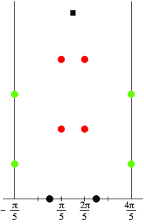
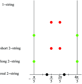
Figure 1: A typical pattern of zeros of a transfer matrix eigenvalue. The four kinds of strings are shown in the analyticity strip within the upper-half complex $u$-plane. The $(1,1)$ boundary condition is on the left and $(1,2)$ on the right. A single $1$-string (shown in black) occurs furthest from the real axis with a fixed location for all eigenvalues in the $(1,1)$ sector. No short $2$-strings (shown in red) occur in the ground states for which the Fermi sea of long $2$-strings (shown in green) is full. A real 2-string (shown in black) occurs on the real axis.

A $1$-string $u_{j}=3\pi/10+iv_{j}$ lies in the middle of the analyticity strip and has real part $3\pi/10$. It occurs only in the $(1,1)$ sector and has a fixed location for all eigenvalues in this sector. A short $2$-string consists of a pair of zeros $u_{j}=\pi/5+iy_{j}$, $2\pi/5+iy_{j}$ with common imaginary parts and real parts $\pi/5$, $2\pi/5$ respectively. The two zeros $u_{j}=-\pi/5+iy_{j}$, $4\pi/5+iy_{j}$ of a long $2$-string have common imaginary parts and real parts $-\pi/5$, $4\pi/5$ respectively so that these zeros sit at the edge of the analyticity strip. Strictly speaking, due to periodicity, long $2$-strings could be considered as $1$-strings. Here, however, we follow the nomenclature used for RSOS models with more than one analyticity strip. Lastly, a real 2-string consists of a pair of zeros $u_{j}=\pi/10,\pi/2$ on the real axis. Usually the real parts of such strings approach these special values for large $N$ but here, because of symmetries, the values of these real parts are exact for finite $N$.

The string contents are described by $(m,n)$ systems Melzer ; Berk94 which, for the Lee-Yang model, take the form

$$\begin{array}[]{rl}&\ \ 2m+n+3-s=N\ \ \Leftrightarrow\ \ m+n=N-m+s-3,\qquad s=1,2\\ &m=\text{\{number of short $2$-strings\}},\qquad n=\text{\{number of long $2$-strings\}}\end{array}$$ (83)

There is always a real 2-string on the real axis and, in the $(r,s)=(1,1)$ sector, a single $1$-string furthest from the real axis. Each short $2$-string contributes two zeros and, by periodicity, each long $2$-string contributes one zero. The 1-string contributes one zero and so does the real 2-string since it is shared between the upper and lower half planes. Consequently, the $(m,n)$ system expresses the conservation of the $2N$ zeros in the periodicity strip. No short $2$-strings occur in the ground states for which the “Fermi sea” of long $2$-strings is full. For finite excitations above the ground state, $m$ is finite but $n\sim N$ as $N\to\infty$.

An excitation with string content $(m,n)$ is uniquely labelled by a set of quantum numbers

$$I=(I_{1},I_{2},\ldots,I_{m})$$ (84)

where the integers $I_{j}\geq 0$ give the number of long 2-strings whose imaginary parts are greater than that of the given short 2-string $y_{j}$. The short 2-strings and long 2-strings labelled by $j=1$ are closest to the real axis. The quantum numbers $I_{j}$ satisfy

$$n\geq I_{1}\geq I_{2}\geq\dots\geq I_{m}\geq 0.$$ (85)

For given string content $(m,n)$, the lowest excitation occurs when all of the short 2-strings are further out from the real axis than all of the long 2-strings. In this case all of the quantum numbers vanish $I_{j}=0$. Bringing the location of a short 2-string closer to the real axis by interchanging the location of the short 2-string with a long 2-string increments its quantum number by one unit and increases the energy.

Finitized characters.

On the lattice it is convenient to work with finitized versions of the Virasoro characters (79) and (81) which converge to them in the $N\to\infty$ limit. These finitized characters are fermionic in the sense that they are given by $q$-polynomials with nonnegative integer coefficients. The finitized characters are

$$(r,s)=(1,1):\ \ \hat{\chi}_{0}^{(N)}(q)=\sum_{m=0}^{\lfloor N/2\rfloor}q^{m^{2}+m}\Big{[}\begin{array}[]{c}N\!-\!1\!-\!m\\ m\end{array}\Big{]}_{q}\to\hat{\chi}_{0}(q)$$ (88)

$$(r,s)=(1,2):\ \ \hat{\chi}_{-1/5}^{(N)}(q)=\sum_{m=0}^{\lfloor N/2\rfloor}q^{m^{2}}\Big{[}\begin{array}[]{c}N\!-\!m\\ m\end{array}\Big{]}_{q}\,\to\,\hat{\chi}_{-1/5}(q)$$ (91)

where the $q$-binomial satisfies

$$\Big{[}\begin{array}[]{c}N\\ m\end{array}\Big{]}_{q}=\,\prod_{i=1}^{m}\frac{1-q^{N+1-i}}{1-q^{i}}\to\,\prod_{i=1}^{m}\frac{1}{1-q^{i}},\qquad N\to\infty$$ (94)

Setting $q=1$ gives the correct counting of states in terms of binomial coefficients

$$\hat{\chi}_{0}^{(N)}(1)=\!\!\sum_{m=0}^{\lfloor N/2\rfloor}\Big{(}\begin{array}[]{c}N\!-\!1\!-\!m\\ m\end{array}\Big{)}=F_{N},\quad\ \ \hat{\chi}_{-1/5}^{(N)}(1)=\!\sum_{m=0}^{\lfloor N/2\rfloor}\Big{(}\begin{array}[]{c}N\!-\!m\\ m\end{array}\Big{)}=F_{N+1}\quad$$ (99)

where the Fibonacci numbers are given by

$$F_{N}=F_{N-1}+F_{N-2}=1,1,2,3,5,8.\ldots,\qquad N=1,2,3,4,5,6,\ldots$$ (100)

The finitized characters can also be written in the form of 1-dimensional configurational sums related to Baxter’s CTMs

$$\hat{\chi}_{h}^{(N)}(q)=\sum_{E}q^{E}=\sum_{\sigma}q^{\sum_{j=1}^{N}jH(\sigma_{j-1},\sigma_{j},\sigma_{j+1})}$$ (101)

where the first sum is over integer conformal energies $E$ and the second sum is over all one-dimensional RSOS paths $\sigma=\{\sigma_{0},\sigma_{1},\ldots,\sigma_{N}\}$ on $A_{4}$ with $\sigma_{0}=s$ and either $(\sigma_{N},\sigma_{N+1})=(2,3)$ or $(\sigma_{N},\sigma_{N+1})=(3,2)$ depending on the parity of $N$. The energy function $H$ is

$$H(\sigma_{j-1},\sigma_{j},\sigma_{j+1})=\begin{cases}1,&(\sigma_{j-1},\sigma_{j},\sigma_{j+1})=(2,1,2)\ \mbox{or}\ (3,4,3)\\ 0,&\text{otherwise}\end{cases}$$ (102)

This local energy function differs from, but is gauge equivalent to, the one used in FB85 . The lowest configuration energy $E=0$ occurs for a ground state RSOS path with heights alternating between 2 and 3.

Bijection between zero patterns and RSOS paths.

              

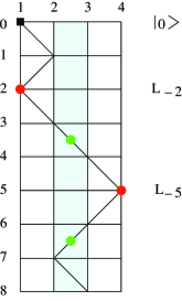
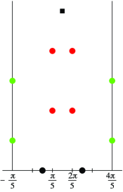
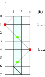
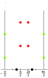
Figure 2: On the left is shown the bijection between one-dimensional configurational paths $\sigma$, strings in the periodicity strip and the Virasoro descendants over $|0\rangle$ or $|h\rangle=|\Phi\rangle=|\!-\frac{1}{5}\rangle$. The paths $\sigma$ are rotated $90^{\circ}$ clockwise and finish with height 2 followed by height 3. The ground states are given by alternation between heights 2 and 3 in the shaded band. On the right is shown the associated patterns of zeros in the analyticity strip. An $(r,s)=(1,1)$ example is shown on the left and an $(r,s)=(1,2)$ example on the right. The $1$-string (solid black square), short $2$-strings (solid red disks) and long $2$-strings (solid green disks) in the upper-half complex $u$-plane are shown maintaining their relative vertical positions. A short 2-string at position $j$ is associated with the Virasoro mode $L_{-j}$ at the given vertical position. For the $(1,1)$ case, the string (particle) content is $m=n=2$ with $N=8$ and modes inserted at $j=2,5$. For the $(1,2)$ case, the string (particle) content is $m=n=2$ with $N=7$ and modes inserted at $j=1,4$. The energies of these excited states are $E=2+5=7$ and $E=1+4=5$ respectively. The corresponding Virasoro sates are $L_{-5}L_{-2}|0\rangle$ and $L_{-4}L_{-1}|h\rangle$ respectively.

There is in fact a bijection FP02 ; FPW between the allowed patterns of strings in the periodicity strip, the one-dimensional RSOS paths $\sigma$ that label the eigenstates (eigenvalues) and Virasoro descendant states. Although this bijection is useful for counting and classifying states, it does not imply that each individual eigenstate is to be identified with the individual Virasoro state. Indeed, there are typically many degenerate levels in any energy eigenspace and, in general, a given eigenstate can only be written as a linear combination with other linearly independent Virasoro states at that energy level. However, the independent eigenstates and Virasoro states are equinumerous within each fixed energy eigenspace.

A simple natural bijection is constructed as follows. A consecutive pair of heights $(\sigma_{j},\sigma_{j+1})=(2,3)$ or $(3,2)$ corresponds to a long $2$-string (dual particle) at position $j+\frac{1}{2}$. The alternation of heights between $2$ and $3$ give the lowest energy configuration and the ground state $|h\rangle$ in a given sector. A triple $(\sigma_{j-1},\sigma_{j},\sigma_{j+1})=(2,1,2)$ or $(3,4,3)$ corresponds to a short $2$-string (particle) at position $j$ and an insertion of a Virasoro mode $L_{-j}$. Because of the RSOS constraints, the particles obey nearest-neighbour exclusion. In addition, in the sector $(r,s)=(1,1)$, there is a single $1$-string at $j=0$ (furthest from the real axis) corresponding to the initial height $s=1$ at $j=0$. This bijection is illustrated in Figure 2. Notice that only the relative positions of the long and short $2$-strings are important. In both cases, the first height is $\sigma_{0}=s$ and the last pair is $(\sigma_{N},\sigma_{N+1})=(2,3)$ with the parity of $N$ fixed accordingly. A particle has an effective diameter of two units whereas a dual particle has a diameter of one unit. We see that the geometric packing constraint

$$2m+n+3-s=N$$ (103)

agrees with the $(m,n)$ system.

Flow between boundary conditions.

Using the boundary conditions (2.2.3), a Renormalization Group (RG) boundary flow is induced from the identity conformal boundary fixed point $\mathbbm{1}=(1,1)$ to the $\Phi=(1,2)$ conformal boundary fixed point as $\mathop{\rm Im}\xi$ increases from $0$ to $\infty$. The boundary entropies AffleckLudwig are given by DPTW ; DRTW

$$g_{\mathbbm{1}}=\Big{(}\frac{\sqrt{5}-1}{2\sqrt{5}}\Big{)}^{\!\frac{1}{4}}\!\!,\ \ g_{\Phi}=\Big{(}\frac{2+\sqrt{5}}{\sqrt{5}}\Big{)}^{\!\frac{1}{4}}\!\!,\ \ \log g_{\mathbbm{1}}^{2}=-0.642965,\ \ \log g_{\mathbbm{1}}g_{\Phi}=-0.161754\quad$$ (104)

The physical flow is from the $\Phi$ boundary fixed point to the identity $\mathbbm{1}$ fixed point so that the boundary entropy decreases along the flow. The mathematical flow we describe is in the opposite direction. It can be described simply in terms of each of the three different descriptions of the states, namely, the zero patterns, the RSOS paths or the Virasoro states.

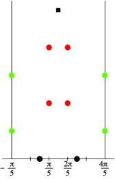
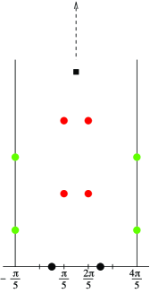
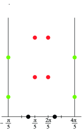
Figure 3: The boundary flow from $\mathbbm{1}=(1,1)$ to $\Phi=(1,2)$ in terms of the flow of zeros. On the left $\xi=0$ while on the right $\xi=i\infty$. For intermediate values of $\xi$, shown in the middle, the 1-string moves continuously to $i\infty$ and disappears. The relative ordering of the 2-strings is not effected.

In terms of the zeros and $(m,n)$ systems, the flow is very simple: the 1-string which only exists for the $(1,1)$ integrable boundary condition migrates vertically off to $i\infty$ as indicated in Figure 3. There is no change in the relative ordering of the 2-string content. The flow in terms of the paths is also simple. We merely have to remove the first step of each of the $(1,1)$ paths to obtain a $(1,2)$ path. More interesting is the flow in terms of the Virasoro modes. First of all, there is a flow $|0\rangle\mapsto|\Phi\rangle$ between the highest weight states. For a Virasoro state, the simple rule is to increase the index of each Virasoro mode by one $L_{-n}\mapsto L_{-n+1}$:

$$L_{-n_{1}}L_{-n_{2}}...L_{-n_{k}}|0\rangle\rightarrow L_{-n_{1}+1}L_{-n_{2}+1}...L_{-n_{k}+1}|\Phi\rangle$$ (105)

This flow is summarized for the first few excited states in Table 1. As expected and shown in the table, the flow interpolates between the reduced characters

$$\hat{\chi}_{0}(q) =1+q^{2}+q^{3}+q^{4}+q^{5}+2q^{6}+2q^{7}+3q^{8}+3q^{9}+...$$ (106)

$$\hat{\chi}_{-\frac{1}{5}}(q) =1+q+q^{2}+q^{3}+2q^{4}+2q^{5}+3q^{6}+3q^{7}+...$$ (107)

The level by level flow agrees with the TCSA results of Dorey et al. DPTW .

Level	State in the $(1,1)$ module	State in the $(1,2)$ module	Level
h.w. state	$|0\rangle$	|$\Phi\rangle$	h.w. state
2	$L_{-2}|0\rangle$	$L_{-1}|\Phi\rangle$	1
3	$L_{-3}|0\rangle$	$L_{-2}|\Phi\rangle$	2
4	$L_{-4}|0\rangle$	$L_{-3}|\Phi\rangle$	3
5	$L_{-5}|0\rangle$	$L_{-4}|\Phi\rangle$	4
6	$L_{-2}L_{-4}|0\rangle$	$L_{-1}L_{-3}|\Phi\rangle$	4
6	$L_{-6}|0\rangle$	$L_{-5}|\Phi\rangle$	5
7	$L_{-2}L_{-5}|0\rangle$	$L_{-1}L_{-4}|\Phi\rangle$	5
7	$L_{-7}|0\rangle$	$L_{-6}|\Phi\rangle$	6
8	$L_{-2}L_{-6}|0\rangle$	$L_{-1}L_{-5}|\Phi\rangle$	6
8	$L_{-3}L_{-5}|0\rangle$	$L_{-2}L_{-4}|\Phi\rangle$	6
8	$L_{-8}|0\rangle$	$L_{-7}|\Phi\rangle$	7
9	$L_{-2}L_{-7}|0\rangle$	$L_{-1}L_{-6}|\Phi\rangle$	7
9	$L_{-3}L_{-6}|0\rangle$	$L_{-2}L_{-5}|\Phi\rangle$	7
9	$L_{-9}|0\rangle$	$L_{-8}|\Phi\rangle$	8

Table 1: The boundary flow induced by $\xi\to i\infty$ described state by state in increasing energy.

3.1.2 Periodic case

For periodic boundary conditions, the excitations are again classified by the patterns of zeros. The known diagonal modular invariant partition function is

$$Z(q)=|\chi_{0}(q)|^{2}+|\chi_{-\frac{1}{5}}(q)|^{2}$$ (108)

Consequently, the states separate into two sectors $(h,\bar{h})=(0,0)$ with $s=\bar{s}=1$ and $(h,\bar{h})=(-{1\over 5},-{1\over 5})$ with $s=\bar{s}=2$ according to whether 1-strings occur at the top and bottom of the analyticity strip or not as shown in Figure 4. If there is a 1-string in the lower half-plane then there is always a 1-string in the upper half-plane. The same 1-strings and short and long 2-strings occur as in the boundary case. In the period case, however, there are no real 2-strings on the real axis although a short 2-string can occur on the real axis. In accord with the diagonal modular invariant, there is a sector selection rule that imposes $s=\bar{s}=1,2$. The main difference in the periodic case, is that the zeros in the lower half plane are not necessarily related to those in the upper half plane except for the fixed 1-strings. It is observed that the patterns of zeros in the upper and lower half-planes occur independently of each other and that each is described by an $(m,n)$ system. The patterns of zeros in the upper and lower half-planes relate to the two chiral halves of the theory.

To classify the states for finite $N$, we use the classification already developed for the boundary case, taking into account that the lower- and upper-half planes are independent, except for a possible real 2-string on the real axis. By convention, this is regarded as occurring in the lower-half plane. For the $(m,n)$ structure, we differentiate between the structures in the upper- and lower-half planes and introduce a doubled $(m,n;\bar{m},\bar{n})$ system. The lattice must now have $2N$ sites around a period. So, if we have a real 2-string (regarded as being in the lower half-plane), then we must have $N-1$ zeros in the upper half-plane and $N$ zeros in the lower half-plane. Otherwise we must have $N$ zeros in each half-plane.

In terms of the RSOS paths, we fix the last step of the path in the upper half-plane to be either $(2,3)$ or $(3,2)$ depending on the parity of $N$. This ensures that the half paths in the upper and lower half-planes both end at the ground state heights corresponding to the shaded band in Figure  4. The contributing characters are $\hat{\chi}_{h}^{(N-1)}(q)=\sum_{E}q^{E}$, as given by (101), in the upper half plane and

$$\hat{\chi}_{h}^{(N)}(\bar{q})=\sum_{E}\bar{q}^{E}=\sum_{\sigma}\bar{q}^{\sum_{j=1}^{N-1}(2N-j)H(\sigma_{j-1},\sigma_{j},\sigma_{j+1})}$$ (109)

in the lower half-plane where $\bar{q}$ denotes the complex conjugate of the modular nome $q$. Generalizing the arguments of Melzer Melzer to this non-unitary theory, the modular invariant partition function admits the finitization

$$Z^{(N)}(q)=\chi_{0}^{(N-1)}(q)\chi_{0}^{(N)}(\bar{q})+\chi_{-\frac{1}{5}}^{(N-1)}(q)\chi_{-\frac{1}{5}}^{(N)}(\bar{q})\to Z(q),\qquad N\to\infty$$ (110)

The correct counting of states follows from the identity

$$Z^{(N)}(1)=F_{N-1}F_{N}+F_{N}F_{N+1}=F_{2N}$$ (111)

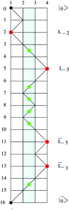
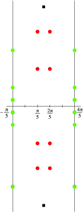
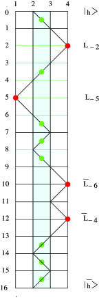
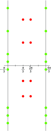
Figure 4: Two typical patterns of zeros for transfer matrix eigenvalues for $N=8$ in the periodic case in the sectors $(0,0)$ and $(-\frac{1}{5},-\frac{1}{5})$ respectively showing the identification between the zeros of the transfer matrix, paths and Virasoro descendants. The ground state alternating band of heights 2 and 3 at the centre can be made arbitrarily long without effecting the energies of the eigenvalues. The paths start at height $s$ in the upper half-plane and finish at height $\bar{s}$ in the lower half-plane. In accord with the diagonal modular invariant, there is a sector selection rule that imposes $s=\bar{s}=1,2$. The cases $s=\bar{s}=3,4$ are equivalent by the $\mathbb{Z}_{2}$ symmetry of the $A_{4}$ diagram.

In the $s=\bar{s}=1$ sector, the state with 1-strings, but with no short 2-strings corresponds to the vacuum state $|0\rangle=|0,0\rangle=|0\rangle\otimes|\bar{0}\rangle$. The state with one short 2-string in the upper half-plane furthest from the real axis corresponds to the state $L_{-2}|0\rangle$. Moving the short 2-string downwards through the long 2-strings increases the level by 1 unit for each permutation, thus creating the $L_{-n}|0\rangle$ state. The mirror image argument applies to the lower half-plane to give states such as $\bar{L}_{-n}|\bar{0}\rangle$. In the $s=\bar{s}=2$ sector, the lowest energy state $|\Phi\rangle=|\!-\frac{1}{5},-\frac{1}{5}\rangle=|\!-\frac{1}{5}\rangle\otimes|\overline{-\frac{1}{5}}\rangle$ has no 1-strings and no short 2-strings. The first excited state in the sector $V_{1}\otimes\bar{V}_{1}$ contains one short 2-string on the top of all long 2-strings and correspond to $L_{-1}|\Phi\rangle$. Every time we lower a short 1-string below a long 2-string we obtain one extra unit of energy, hence we generate all the $L_{-n}|\Phi\rangle$ and similarly for the lower half plane with $\bar{L}_{-n}$ Virasoro modes. These correspondences between Virasoro descendants, RSOS paths and the zero patterns can be read off from Figure 4.

3.1.3 Periodic boundary condition with a seam

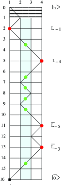
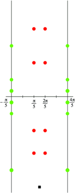
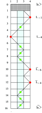
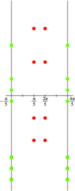
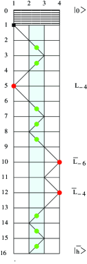
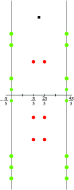
Figure 5: Identification, for the seam transfer matrix eigenvalues, between the zero patterns, RSOS paths and Virasoro modes in the case of an $(r,s)=(1,2)$ seam ($\xi\to i\infty$). The heights across the seam differ by $\pm 1$. The RSOS paths are restricted to pass through the shaded ground-state band at the level of the real axis. The remaining RSOS paths are related to these by the $\mathbb{Z}_{2}$ $A_{4}$ symmetry.

Consider the periodic transfer matrix (33) with a simple seam with parameter $\xi$. By varying $\xi$ from $0$ to $i\infty$, the two endpoints are described as follows: for $\xi=0$ we have the $(r,s)=(1,1)$ identity seam which disappears, so we recover the results of the periodic boundary condition analyzed in the previous subsection. In the $\xi\to i\infty$ limit, which gives the $(r,s)=(1,2)$ seam, we find the identification between string patterns, RSOS paths and Virasoro modes summarized in Figure 5. Comparing with the periodic case we can see that, in the $\xi=i\infty$ limit, the sector selection rule is that a 1-string can appear either in the lower or in the upper half plane but not in both. The identification is otherwise as in the periodic case but the Hilbert space in the $N\to\infty$ limit is

$$\mathcal{H}=V_{0}\otimes\bar{V}_{-\frac{1}{5}}+V_{-\frac{1}{5}}\otimes\bar{V}_{0}+V_{-\frac{1}{5}}\otimes\bar{V}_{-\frac{1}{5}}$$ (112)

corresponding to the twist partition function

$$Z_{\text{\tiny seam}}(q)=\chi_{0}(q)\chi_{-\frac{1}{5}}(\bar{q})+\chi_{-\frac{1}{5}}(q)\chi_{0}(\bar{q})+\chi_{-\frac{1}{5}}(q)\chi_{-\frac{1}{5}}(\bar{q})$$ (113)

with the finitized version

$$Z_{\text{\tiny seam}}^{(N)}(q)=\chi_{0}^{(N-1)}(q)\chi_{-\frac{1}{5}}^{(N-1)}(\bar{q})+\chi_{-\frac{1}{5}}^{(N-1)}(q)\chi_{0}^{(N-1)}(\bar{q})+\chi_{-\frac{1}{5}}^{(N-1)}(q)\chi_{-\frac{1}{5}}^{(N-1)}(\bar{q})$$ (114)

The correct counting of states follows from the identity

$$Z_{\text{\tiny seam}}^{(N)}(1)=F_{N-1}F_{N}+F_{N}F_{N-1}+F_{N}^{2}=F_{2N}$$ (115)

The corresponding Virasoro highest weights states are denoted by $|{\phi}\rangle$, $|\bar{\phi}\rangle$ and $|\Phi\rangle$ respectively. In the language of 1-d configurational sums, we see that the contributing part of the RSOS paths is not periodic. Instead, the heights across the seam differ by $\pm 1$ in accord with the weights of the $(1,2)$ seam (36).

Seam flow.

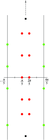
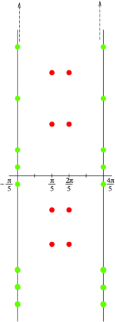
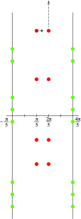
Figure 6: Depending on the outermost configurations the three different mechanisms A, B, C, which appear in the flow $\xi\to i\infty$.

We can analyse the flow in $\xi$ in terms of the various descriptions as indicated. In terms of the zeros, we identify three mechanisms depending on the sector:

1. If the outermost string is a 1-string, it flows to infinity (in the same half-plane) as $\xi\to i\infty$.

2. If the outermost string is a long 2-string, it flows to infinity (in the same half-plane) as $\xi\to i\infty$.

3. If the outermost string is a short 2-string, one of the zeros flows to infinity (in the same half-plane) and the other becomes a 1-string with real part $\frac{3\pi}{10}$.

These mechanisms, shown in the left, middle and right respectively in Figure 6, are similar to the three mechanisms observed FPR for the boundary flow in the tricritical Ising model.

In terms of Virasoro states, this is summarized as:

1. Due to type A flows with $|0\rangle\rightarrow|\bar{\phi}\rangle$:

   $$L_{-N_{1}}...L_{-N_{n}}\bar{L}_{-\bar{N}_{1}}....\bar{L}_{-\bar{N}_{n}}|0\rangle\rightarrow L_{-N_{1}}...L_{-N_{n}}\bar{L}_{-\bar{N}_{1}+1}....\bar{L}_{-\bar{N}_{n}+1}|\bar{\phi}\rangle$$

2. Due to type B flows with $|\Phi\rangle\rightarrow|{\Phi}\rangle$:

   $$L_{-N_{1}}...L_{-N_{n}}\bar{L}_{-\bar{N}_{1}}....\bar{L}_{-\bar{N}_{n}}|\Phi\rangle\rightarrow L_{-N_{1}}...L_{-N_{n}}\bar{L}_{-\bar{N}_{1}+1}...\bar{L}_{-\bar{N}_{n}+1}|\Phi\rangle$$

3. Due to type C flows with $|\Phi\rangle\rightarrow|{\phi}\rangle$:

   $$(L_{-N_{1}}...L_{-N_{n}}\bar{L}_{-\bar{N}_{1}}....\bar{L}_{-\bar{N}_{n}})\bar{L}_{-1}|\Phi\rangle\rightarrow(L_{-N_{1}}...L_{-N_{n}}\bar{L}_{-\bar{N}_{1}+1}....\bar{L}_{-\bar{N}_{n}+1})|\phi\rangle$$

The three mechanisms for the flow of the patterns of zeros are confirmed numerically. It follows that the flow, under the three mechanisms, of the first few states of the identity defect as in Figure 6 is as shown in Table 2.

Level	Trivial Defect	Non-trivial Defect	Level
h.w. state	$|0\rangle$	|$\bar{\phi}\rangle$	h.w. state
h.w. state	|$\Phi\rangle$	|$\Phi\rangle$	h.w. state
1	$\bar{L}_{-1}|\Phi\rangle$	$|\phi\rangle$	h.w. state
1	$L_{-1}|\Phi\rangle$	$L_{-1}|\Phi\rangle$	1
2	$\bar{L}_{-2}|0\rangle$	$\bar{L}_{-1}$$|\bar{\phi}\rangle$	1
2	$\bar{L}_{-2}|\Phi\rangle$	$\bar{L}_{-1}|\Phi\rangle$	1
2	$\bar{L}_{-1}L_{-1}|\Phi\rangle$	$L_{-1}|\phi\rangle$	1
2	$L_{-2}|\Phi\rangle$	$L_{-2}|\Phi\rangle$	2
2	$L_{-2}|0\rangle$	$L_{-2}|\bar{\phi}\rangle$	2
3	$\bar{L}_{-3}|0\rangle$	$\bar{L}_{-2}$$|\bar{\phi}\rangle$	2
3	$\bar{L}_{-3}|\Phi\rangle$	$\bar{L}_{-2}|\Phi\rangle$	2
3	$\bar{L}_{-2}L_{-1}|\Phi\rangle$	$\bar{L}_{-1}L_{-1}|\Phi\rangle$	2
3	$\bar{L}_{-1}L_{-2}|\Phi\rangle$	$L_{-2}|\phi\rangle$	2
3	$L_{-3}|\Phi\rangle$	$L_{-3}|\Phi\rangle$	3
3	$L_{-3}|0\rangle$	$L_{-3}|0\rangle$	3
4	$\bar{L}_{-1}\bar{L}_{-3}|\Phi\rangle$	$\bar{L}_{-2}|\phi\rangle$	2

Table 2: The flow from each state in the trivial identity defect Hilbert space to its corresponding state in the non-trivial defect Hilbert space up to the second order descendent level in the defect Hilbert space.

As expected from defect CFT, the flow is

$$V_{0}\otimes\bar{V}_{0}+V_{-\frac{1}{5}}\otimes\bar{V}_{-\frac{1}{5}}\ \mapsto\ V_{0}\otimes\bar{V}_{-\frac{1}{5}}+V_{-\frac{1}{5}}\otimes\bar{V}_{0}+V_{-\frac{1}{5}}\otimes\bar{V}_{-\frac{1}{5}}$$ (116)

Taking instead the limit $\xi\rightarrow-i\infty$ gives a similar result but with $\phi$ and $\bar{\phi}$ interchanged and $L_{-n}$ being the operator augmented to $L_{-n+1}$ instead of the $\bar{L}_{-n}$ modes. The corresponding physical flows were confirmed level by level using defect TCSA in Bajnok:2013waa .

3.2 Continuum scaling limit in the critical case

In this section, for the critical case, we explain how the distribution of zeros scale in the continuum scaling limit for finite energy states. As $N\to\infty$ the spacing of the zeros becomes more dense. Quantitatively, the imaginary part of the outer most zeros grow as $\frac{3}{5}\log N$ so the spacing between zeros shrinks to $0$ as $\frac{3}{5}\frac{\log N}{N}$. The pattern of zeros for a finite energy state is shown schematically in Figure 7. The imaginary part of the 1-string is denoted by $\alpha$, while the imaginary part of the short 2-strings are denoted by $\beta_{j}$. There are a finite number of short 2-string excitations. The $\alpha$ and $\beta_{j}$ variables together with the imaginary parts of the long 2-strings furthest from the real axis all scale as $\frac{3}{5}\log N$ in the continuum scaling limit. These configurations correspond to Virasoro descendants with a finite number of Virasoro modes and to paths which, except over a finite interval, alternate between heights $2$ and $3$. Similar observations apply for periodic boundary conditions, with or without a seam, except that the patterns in the upper and lower half of the plane need not be the same. In the continuum scaling limit, the zeros in the scaling regions in the upper and lower half-planes are effectively “infinitely far” from each other and thus independent of each other.

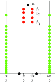
Figure 7: Pattern of zeros of a finite excitation for large $N$ showing the scaling region a distance $\frac{3}{5}\log N$ out from the real axis.

3.3 Classification of states in the off-critical theory

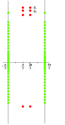
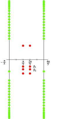
Figure 8: Periodicity of the off-critical transfer matrix brings the scaling regions in the upper and lower half-planes close to each other across the boundary of the period rectangle. On the left, the massive zeros are shown using the variable $u$, while on the right, the shifted variable $u+\frac{1}{2}\log q$ is used.

In the off-critical theory, the Boltzmann weights are given in terms of the elliptic function $s(u)=\vartheta_{1}(u,q)$. Unlike the sine function, this elliptic function is quasi-periodic in the imaginary direction

$$\vartheta_{1}(u+\pi,q)=-\vartheta_{1}(u,q),\qquad\vartheta_{1}(u-i\log q,q)=-q^{-1}e^{-2iu}\vartheta_{1}(u,q)$$ (117)

It follows that the eigenvalues of the transfer matrices in the various geometries are entire functions of $u$ in the period rectangle

$$\mbox{period rectangle}=\{\mathop{\rm Re}u\in[-\tfrac{\pi}{5},\tfrac{4\pi}{5}],\ \mathop{\rm Im}u\in[-\tfrac{1}{2}\log q,\tfrac{1}{2}\log q]\}$$ (118)

We can therefore restrict our analysis to this period rectangle. Moreover, within this period rectangle, the eigenvalues are completely characterized by their zeros. Actually the renormalized transfer matrices are periodic in this period rectangle.

We are interested in the massive Lee-Yang model which is the continuum scaling limit of the off-critical lattice Lee-Yang model. The parameter $q^{2}$ measures the departure from criticality. As we will see, we have to tune the square of the elliptic nome as $q^{2}\propto N^{-5/3}$ as $N\to\infty$ for the continuum scaling limit to exist. Numerically, for reasonable sizes of $N$, we find that the locations of the zeros in the complex $u$-plane follow the same patterns found in the critical case. The observed deviations from the critical locations are exponentially small in $N$. What is conceptually different is that, while in the critical case the upper and lower scaling regions are “infinitely far” apart, in the massive case periodicity glues them together as shown in Figure 8.

4 Critical TBA Equations

In this section we exploit the analytic structure of the transfer matrix eigenvalues to turn the functional relation (22) into TBA integral equations. We start by reviewing the critical case with periodic boundary conditions before adding a seam and moving to the massive case. In the periodic critical case, the central charge and conformal dimension of the single non-trivial primary field were calculated analytically in BLZ following the methods of KlumP91 ; KlumP92 .

4.1 Critical TBA

The critical TBA equations are derived by solving the functional relation

$$t(u)t(u+\lambda)=1+t(u+3\lambda)$$ (119)

taking into account the analytic structure of the function $t(u)$. The function $t(u)$ is factorized according to its large volume behaviour as

$$t(u)=f(u)g(u)l(u)$$ (120)

where $\log f(u)=O(N)$, $\log g(u)=O(1)$ and $\log l(u)=O(N^{-1})$. The leading order term satisfies

$$f(u)f(u+\lambda)=1$$ (121)

and accounts for the order $N$ zeros and poles of the normalization. The function $g(u)$ also satisfies

$$g(u)g(u+\lambda)=1$$ (122)

and accounts for the order $1$ boundary- and seam-dependent zeros and poles. An integral equation is derived for the remaining finite-size function $l(u)$.

4.1.1 Periodic case

The energy of the states is extracted from the finite-size corrections of the transfer matrix eigenvalues

$$\log t(u)=\log f(u)+\log g(u)-\frac{i}{N}(e^{-\frac{5i}{3}u}E^{+}-e^{\frac{5i}{3}u}E^{-})$$ (123)

For physical values of $u$ with $0<u<{3\pi\over 5}$, the first term in the ${1\over N}$ correction dominates when $u\to+i\infty$ and the second term when $u\to-i\infty$. The finite-size conformal Lee-Yang energies are

$$E_{LY}=e^{x}E^{+}+e^{-x}E^{-},\qquad u=\frac{\lambda}{2}+\frac{3ix}{5}$$ (124)

These energies can be calculated analytically following the methods of KlumP91 ; KlumP92 .

As the analytic structure of the two sectors are different, we start with the simpler $(r,s)=(1,2)$ or $|\Phi\rangle$ sector, which contains the lowest energy state or “true vacuum”. For periodic boundary conditions, the number of faces $N$ is even. Using the periodicity of the transfer matrix $t(u)=t(u+\pi)$, after an appropriate shift, we obtain

$$t(u-\frac{\pi}{5})t(u+\frac{\pi}{5})=1+t(u)$$ (125)

The normalization (29) introduces order $N$ zeros at $-\frac{\pi}{5},\frac{4\pi}{5}$ and order $N$ poles at $\frac{\pi}{5},\frac{2\pi}{5}$. We remove them by normalizing with the function $f(u)$ which satisfies

$$f(u-\frac{\pi}{5})f(u+\frac{\pi}{5})=f(u)$$ (126)

The solution compatible with the analytic structure is

$$f(u)=f_{1}(u)^{N}=\Big{(}\frac{\sin\frac{5u}{3}+\sin\frac{\pi}{3}}{\sin\frac{5u}{3}-\sin\frac{\pi}{3}}\Big{)}^{N}=\Big{(}\!-\frac{\sin(\frac{5u}{6}+\frac{\pi}{6})\sin(\frac{5u}{6}+\frac{2\pi}{6})}{\cos(\frac{5u}{6}+\frac{\pi}{6})\cos(\frac{5u}{6}+\frac{2\pi}{6})}\Big{)}^{N}$$ (127)

Observe that this solution also satisfies $f(u)f(u+\lambda)=1$ as anticipated in (121). In the periodic case, there is no order $1$ boundary contribution so $g(u)=1$.

In the large $N$ limit, the imaginary part of the position of the long 2-string furthest from the real $u$ axis approaches infinity as $\frac{3}{5}\log\kappa N$ with

$$\kappa=4\sin\frac{\pi}{3}=2\sqrt{3}$$ (128)

This motivates introducing the real variable $x$ as a scaled vertical coordinate along the centre of the analyticity strip

$$u=\frac{3\pi}{10}+\frac{3ix}{5}$$ (129)

In terms of $x$, the functional equation takes the form

$$t(x-i\frac{\pi}{3})t(x+i\frac{\pi}{3})=1+t(x)$$ (130)

In this variable

$$f(x)=\left(\frac{\cosh x+\sin\frac{\pi}{3}}{\cosh x-\sin\frac{\pi}{3}}\right)^{N}$$ (131)

Vacuum state.

Focusing on the ground state, we divide (130) by $t(x)$ and use the properties of the function $f(x)$ to obtain the standard scaling Lee-Yang $Y$-system

$$\frac{t(x-i\frac{\pi}{3})t(x+i\frac{\pi}{3})}{t(x)}=\frac{l(x-i\frac{\pi}{3})l(x+i\frac{\pi}{3})}{l(x)}=1+{1\over t(x)}$$ (132)

Due to our construction $l(x)$ is Analytic and Non-Zero in the analyticity strip $\mathop{\rm Im}x\in(-\frac{5\pi}{6},\frac{5\pi}{6})$ and its logarithm has Constant asymptotic (ANZC) as $x\to\pm\infty$. Following KlumP91 ; KlumP92 , we can thus take the logarithm and solve the equation using Fourier transforms of the derivatives $[\log l(x)]^{\prime}$ and so on. Evaluating the constants introduced by integrating gives

$$\log l(x)=-\varphi\star\log\Big{(}1+{1\over t(x)}\Big{)},\quad\varphi(x)=-{4\sqrt{3}\cosh x\over 1+2\cosh 2x},\quad\hat{\varphi}=\frac{1}{1-e^{k\frac{\pi}{3}}-e^{-k\frac{\pi}{3}}}$$ (133)

where the convolution is defined by

$$(f\star g)(x)=(g\star f)(x)={1\over 2\pi}\int_{-\infty}^{\infty}f(x-y)g(y)dy$$ (134)

Observe that the kernel $\varphi(x)$ is related to the known CardyMuss89 two-particle $S$-matrix (1) of the Lee-Yang model as $\varphi=-i\partial_{x}\log S(x)$.

We thus obtain the critical TBA equation on the lattice for the ground state with periodic boundary conditions

$$\log t(x)=\log f(x)-\varphi\star\log\Big{(}1+{1\over t(x)}\Big{)}$$ (135)

We are interested in the continuum scaling limit with $N\to\infty$. Analysing the scaling limit of the function $f(x)$, one can see that nontrivial behaviours occur in the two scaling regions $x\sim\pm\log\kappa N$. It is thus natural to introduce two scaling functions

$$e^{\epsilon^{\pm}(x)}=\lim_{N\to\infty}t(x\pm\log\kappa N)$$ (136)

which relate to the left and right chiral halves of the theory. Using the explicit form of the source term $f(x)$, we obtain the behavior in the two scaling regions

$$\lim_{N\to\infty}\log f(x\pm\log\kappa N)=\lim_{N\to\infty}N\log(1+e^{\mp x}\frac{1}{N})=e^{\mp x}$$ (137)

which leads to the massless TBA equations

$$\epsilon^{\pm}(x)=e^{\mp x}-\varphi\star\log(1+e^{-\epsilon^{\pm}(x)})$$ (138)

As the ground state is symmetric under $x\leftrightarrow-x$, we see that $\epsilon^{+}(x)=\epsilon^{-}(x)=\epsilon(x)$ for the ground state. Although this symmetry holds for spinless primary states, it is not generally true for excited states.

Energies.

The two scaling regions contribute to the energy of a general state through $E^{\pm}$, which can be extracted from $\log l(x)$ using (123) and (124)

$$\frac{1}{N}\,(e^{x}E^{+}+e^{-x}E^{-}) = -\log l(x)=\int_{-\infty}^{\infty}\frac{dy}{2\pi}\,\varphi(x-y)\log\Big{(}1+{1\over t(y)}\Big{)}$$ (139)

$$= \left\{\int_{0}^{\infty}+\int_{-\infty}^{0}\right\}\frac{dy}{2\pi}\,\varphi(x-y)\log(1+e^{-\epsilon(y)})$$

We focus first on the $E^{+}$ contribution coming from the $x\to+\infty$ scaling region and the integral $\int_{0}^{\infty}$. By shifting the integrals $y\mapsto y+\log\kappa N$ we can write

$$e^{x}E^{+}=N\int_{-\log\kappa N}^{\infty}\frac{dy}{2\pi}\,\varphi(x-y-\log\kappa N)\log(1+e^{-\epsilon(y+\log\kappa N)})$$ (140)

In the $N\to\infty$ limit

$$\lim_{N\to\infty}N\varphi(x-\log\kappa N)=-\lim_{N\to\infty}\frac{\kappa N\cosh(x-\log\kappa N)}{\cosh(2x-2\log\kappa N)-\cos\frac{2\pi}{3}}=-e^{x}$$ (141)

which leads to

$$E^{+}=-\int_{-\infty}^{+\infty}\frac{dy}{2\pi}\,e^{-y}\log(1+e^{-\epsilon^{+}(y)})$$ (142)

A similar calculation based on the integral $\int_{-\infty}^{0}$ gives the result

$$E^{-}=-\int_{-\infty}^{+\infty}\frac{dy}{2\pi}\,e^{y}\log(1+e^{-\epsilon^{-}(y)})$$ (143)

Central charge.

Consider the ground state TBA with $\epsilon^{+}(x)=\epsilon^{-}(x)=\epsilon(x)$ and set

$$a(x)={1\over t(x)}=e^{-\epsilon(x)},\quad A(x)=1+a(x),\quad\ell a=\log a(x),\quad\ell A=\log A(x)$$ (144)

Then differentiating the TBA gives

$$-\ell a(x)=e^{-x}-\varphi\star\ell A,\qquad-\ell a^{\prime}(x)=-e^{-x}-\varphi\star\ell A^{\prime}$$ (145)

The solution of this TBA has flat plateaus in the asymptotic regions as $x\to\pm\infty$. The asymptotic values are

$$a(\infty)={2\over\sqrt{5}+1}={\sqrt{5}-1\over 2},\qquad a(-\infty)=0$$ (146)

Indeed, using the fact that

$$\int_{-\infty}^{\infty}\!\frac{dy}{2\pi}\,\varphi(y)=-1$$ (147)

it is easily checked that the asymptotic value of $a=a(+\infty)$ must be a solution of ${1\over a}=1+a$.

Next, using the fact that the kernel is even $\varphi(x)=\varphi(-x)$, integrating by parts and changing the integration variable to $a$, it follows that

$$\int_{-\infty}^{\infty}\!\!dy\,[\ell a^{\prime}(y)\ell A(y)-\ell a(y)\ell A^{\prime}(y)]=\int_{-\infty}^{\infty}\!\!dy\,e^{-y}[\ell A(y)-\ell A^{\prime}(y)]=2\int_{-\infty}^{\infty}\!\!dy\,e^{-y}\ell A(y)=\quad$$

$$-4\pi E^{+}=\int_{a(-\infty)}^{a(\infty)}da\Big{[}{\log(1+a)\over a}-{\log a\over 1+a}\Big{]}=2L_{+}\Big{(}{\sqrt{5}-1\over 2}\Big{)}=2L\Big{(}{3-\sqrt{5}\over 2}\Big{)}={2\pi^{2}\over 15}$$ (148)

where the Rogers dilogarithm functions are defined by

$$L(x) =-{1\over 2}\int_{0}^{x}\!\!da\Big{[}{\log(1-a)\over a}+{\log a\over 1-a}\Big{]}$$ (149)

$$L_{+}(x) ={1\over 2}\int_{0}^{x}\!\!da\Big{[}{\log(1+a)\over a}-{\log a\over 1+a}\Big{]}=L\Big{(}{x\over 1+x}\Big{)}$$ (150)

This gives the value of the energy integrals $E^{+}=E^{-}$. In particular, at the isotropic point with $u={\lambda\over 2}={3\pi\over 10}$ and $x=0$, we find the effective central charge

$$E_{LY}=E^{+}+E^{-}=2E^{+}=-{\pi\over 15}=-{\pi c_{\text{\tiny eff}}\over 6},\qquad c_{\text{\tiny eff}}={2\over 5}$$ (151)

Hence the central charge is

$$c=c_{\text{\tiny eff}}+24h_{\text{\tiny min}}={2\over 5}-{24\over 5}=-{22\over 5},\qquad h_{\text{\tiny min}}=-{1\over 5}$$ (152)

Excited states.

The eigenvalues of the transfer matrix are characterized by their patterns of zeros in the analyticity strip $-{\pi\over 5}<\mathop{\rm Re}u<{4\pi\over 5}$. For all eigenvalues, long 2-strings occur at the boundaries $\mathop{\rm Re}u=-{\pi\over 5},{4\pi\over 5}$ of this analyticity strip. In the thermodynamic limit $N\to\infty$, these 2-strings become dense defining the boundaries of the analyticity strip. For finite excitations above the ground state, additional short 2-strings can occur at

$$u_{j}=\begin{cases}\frac{\pi}{5}+i\beta_{j}\\ \frac{2\pi}{5}+i\beta_{j}\end{cases}$$ (153)

Depending on the sector, single 1-strings can also occur furthest out from the real $u$ axis in the upper- and lower-half $u$-plane at

$$u_{0}=\frac{3\pi}{10}+i\alpha$$ (154)

In the scaling regions, at the edge of the distributions of zeros, in the upper/lower half $u$-plane respectively, the zeros approach infinity in the thermodynamic limit as

$$\alpha=\frac{3}{5}(\pm\log\kappa N+\tilde{\alpha}^{\mp}),\qquad\beta_{j}=\frac{3}{5}(\pm\log\kappa N+\tilde{\beta}_{j}^{\mp})$$ (155)

This was checked numerically out to the system size $N=16$.

In the $x=\frac{5}{3i}(u-\frac{3\pi}{10})$ variable, the zeros of the 1-strings are located at

$$x_{0}^{\pm}=\frac{5\alpha}{3}=\pm\log\kappa N+\tilde{\alpha}^{\mp}$$ (156)

and the zeros of the short 2-strings are located at

$$(x_{j}^{\pm}+\frac{i\pi}{6},x_{j}^{\pm}-\frac{i\pi}{6})\quad;\qquad x_{j}^{\pm}=\pm\log\kappa N+\tilde{\beta}_{j}^{\mp}$$ (157)

We need to convert the lattice functional equations into TBA integral equations, solve by Fourier transforms and then take the continuum scaling limit. To do so we need ANZC functions that are free of zeros and poles in an open strip containing $\mathop{\rm Im}x\in[-\frac{\pi}{3},\frac{\pi}{3}]$. The function which removes the single zero introduced by a 1-string is

$$\sigma_{0}(x)=\tanh\frac{3x}{4}$$ (158)

while the one which removes the two zeros of a short 2-string is

$$\sigma_{1}(x)=\frac{\cosh x-\sin\frac{\pi}{3}}{\cosh x+\sin\frac{\pi}{3}}$$ (159)

These functions satisfy BLZ

$$\sigma_{0}(x-\frac{i\pi}{3})\sigma_{0}(x+\frac{i\pi}{3})=1,\qquad\sigma_{1}(x-\frac{i\pi}{3})\sigma_{1}(x+\frac{i\pi}{3})=\sigma_{1}(x)$$ (160)

We therefore parametrize the normalized transfer matrix eigenvalue as

$$t(x)=f(x)\prod_{\pm}\sigma_{0}(x-x_{0}^{\pm})\prod_{j=1}^{M}\sigma_{1}(x-x_{j}^{\pm})\,l(x)$$ (161)

which ensures that $l(x)$ is ANZC in the analyticity strip $\mathop{\rm Im}x\in(-\frac{5\pi}{6},\frac{5\pi}{6})$.

After removing the zeros, the functional equation takes the form

$$\prod_{\pm}\sigma_{0}(x-x_{0}^{\pm})\frac{t(x-i\frac{\pi}{3})t(x+i\frac{\pi}{3})}{t(x)}=\frac{l(x-i\frac{\pi}{3})l(x+i\frac{\pi}{3})}{l(x)}=\prod_{\pm}\sigma_{0}(x-x_{0}^{\pm})\Big{(}1+{1\over t(x)}\Big{)}$$ (162)

Notice that the combination $\prod_{\pm}\sigma_{0}(x-x_{0}^{\pm})/t(x)$ is regular at $x=x_{0}^{\pm}.$ Taking the logarithm and using Fourier transforms again we find

$$\log l(x)=-\varphi\star\log\Big{[}\prod_{\pm}\sigma_{0}(x-x_{0}^{\pm})\Big{(}1+{1\over t(x)}\Big{)}\Big{]}$$ (163)

Restoring $t(x)$ gives

$$\log t(x)\!=\!\log f(x)+\sum_{\pm}\log\sigma_{0}(x-x_{0}^{\pm})+\sum_{j,\pm}\log\sigma_{1}(x-x_{j}^{\pm})-\varphi\star\log\Big{[}\prod_{\pm}\sigma_{0}(x-x_{0}^{\pm})\Big{(}1+{1\over t(x)}\Big{)}\Big{]}$$ (164)

The parameters of the excited state $x_{i}=\{x_{0}^{\pm},x_{j}^{\pm}\}$ are determined self-consistently from the fact that they are zeros of the transfer matrix:

$$t(x)\Big{|}_{x=x_{i}\pm\frac{i\pi}{3}}=-1$$ (165)

In the scaling limit, we focus on the two scaling domains at $\pm\log\kappa N$ by introducing

$$e^{\epsilon^{\mp}(x)}=\lim_{N\to\infty}\sigma_{0}(x\pm\log\kappa N-x_{0}^{\pm})^{-1}t(x+\log\kappa N)$$ (166)

It satisfies the equation

$$\epsilon^{\mp}(x)=e^{\mp x}+\sum_{j}\log\sigma_{1}(x-\tilde{\beta}_{j}^{\mp})-\varphi\star\log(\sigma_{0}(x-\tilde{\alpha}^{\mp})+e^{-\epsilon^{\mp}(x)})$$ (167)

The location of the zeros $\tilde{\alpha}^{\pm}$ and $\tilde{\beta}_{j}^{\pm}$ are self-consistently determined from the following equations

$$e^{\epsilon^{\pm}(x)}\sigma_{0}(x)\Big{|}_{x=\gamma^{\pm}\pm\frac{i\pi}{3}}=-1$$ (168)

where $\gamma^{\pm}$ is either $\tilde{\alpha}^{\pm}$ or $\tilde{\beta}_{j}^{\pm}.$

The contribution of the roots to the energy can be calculated as before

$$E^{\pm}=\sum_{j}e^{\pm\tilde{\beta}_{j}^{\pm}}-\int_{-\infty}^{+\infty}\frac{dx}{2\pi}e^{\mp x}\log(1+e^{-\epsilon^{\mp}(x)})$$ (169)

4.1.2 Periodic case with a seam

In this section we point out the differences, in the case of a seam, compared to the periodic case. The normalization used to bring the fusion equation into the universal form

$$t(u)t(u+\lambda)=1+t(u+3\lambda)$$ (170)

introduces order $N-1$ zeros at $-\frac{\pi}{5},\frac{4\pi}{5}$ and order $N-1$ poles at $\frac{\pi}{5},\frac{2\pi}{5}$. Additionally, a single zero is introduced at $-\frac{\pi}{5}-\xi\equiv\frac{4\pi}{5}-\xi$, and a short 2-string at $\frac{\pi}{5}-\xi,\frac{2\pi}{5}-\xi$ . To be able to describe the flow, we will take $\xi$ to be pure imaginary. The bulk and seam dependent non-universal functions can be factored out as in (120) and we seek an integral equation for $l$. The functions $f(u)$ and $g(u)$, which remove the order $N$/order $1$ zeros and poles are found to be

$$f(u)=f_{1}(u)^{N-1},\qquad g(u)=f_{1}(u+\xi)$$ (171)

In addition to (121) and (122), they also satisfy

$$f(u+\tfrac{\pi}{5})f(u-\tfrac{\pi}{5})=f(u),\qquad g(u+\tfrac{\pi}{5})g(u-\tfrac{\pi}{5})=g(u)$$ (172)

Vacuum state.

For the ground state without 1-strings, following the previous derivation (132) based on the parametrization (120), we obtain the equation

$$\log t(x)=\log f(x)+\log g(x)-\varphi\star\log(1+t^{-1}(x))$$ (173)

This is the ground-state TBA on the lattice with a seam.

In the continuum scaling limit, the contributions come from the scaling regions in the upper half-plane around $x\sim\log\kappa N$ and in the lower half-plane around $x\sim-\log\kappa N$. If we do not scale the parameter $\xi$ with $N$, it disappears from the equations in the scaling limit. So we need to scale it by $\pm i\frac{3}{5}\log N$ to bring the order 1 zeros into the scaling region. It then only appears in the equations for $\epsilon^{\pm}$. Let us consider the scaling region in the upper half-plane with $\xi=\frac{3}{5i}(\tilde{\xi}+\log\kappa N$) and center the new functions around $x\pm\log\kappa N$ as $e^{\epsilon^{\mp}(x)}=\lim_{N\to\infty}t(x\pm\log\kappa N)$. Taking the continuum scaling limit $N\to\infty$ on the source term, we obtain the massless ground-state TBA equations in the presence of a seam

$$\epsilon^{\pm}(x)=e^{\pm x}+\log g(x-\tilde{\xi})-\varphi\star\log(1+e^{-\epsilon^{\pm}(x)})$$ (174)

It is enlightening to compare this result to the massless limit of the defect TBA equation BS . We find that the function $g$ is related to the defect transmission factor $T_{-}(x,b)$ as

$$g(x-\tilde{\xi})=T_{-}(\frac{i\pi}{2}+x,b),\qquad b=3+\frac{6i\tilde{\xi}}{\pi}$$ (175)

In calculating the energy of the ground-state we see that $g$ only contributes to the seam energy and so formulas (142) and (143) for $E^{\pm}$ still hold. The extension of this analysis for excited states is straightforward by including the source term $\log g(x-\tilde{x})$ into (164).

4.1.3 Boundary case

In this section, we consider the ground state and, specifically, the ground-state in the two sectors labeled as $s=1,2$. In this case, the boundary normalization (75) introduces order $2N$ zeros at $-\frac{\pi}{5},\frac{4\pi}{5}$ and order $2N$ poles at $\frac{\pi}{5},\frac{2\pi}{5}$. These are removed by

$$f(u)=f_{1}(u)^{2N}$$ (176)

The boundary normalization (75) introduces a double zero at $u=\frac{\lambda}{2}$, poles at $u=-\frac{\lambda}{2}+\pi=\frac{7\pi}{10}$ and $u=\frac{3\lambda}{2}-\pi=-\frac{\pi}{10}$. Observe that the argument of the order $1$ normalization factor in (75) is $2u$, thus its periodicity is $\frac{\pi}{2}$, which introduces poles at $\frac{\pi}{5}$ and $\frac{2\pi}{5}$. In addition, there is a real 2-string with zeros occurring at $\frac{\pi}{10}$ and $\frac{\pi}{2}$. The factor that satisfies

$$g_{1}(u+\tfrac{\pi}{5})g_{1}(u-\tfrac{\pi}{5})=g_{1}(u)$$ (177)

to remove these zeros and poles is

$$g_{1}(u)=-\frac{\tan^{2}(\frac{5u}{6}-\frac{\pi}{4})\tan(\frac{5u}{6}-\frac{\pi}{12})\tan(\frac{5u}{6}-\frac{5\pi}{12})}{\tan(\frac{5u}{6}-\frac{\pi}{6})\tan(\frac{5u}{6}-\frac{\pi}{3})}$$ (178)

In the $x$ variable it takes the form

$$g_{1}(x)=-\frac{\tan^{2}(\frac{ix}{2})\tan(\frac{ix}{2}+\frac{\pi}{6})\tan(\frac{ix}{2}-\frac{\pi}{6})}{\tan(\frac{ix}{2}-\frac{\pi}{12})\tan(\frac{ix}{2}+\frac{\pi}{12})}$$ (179)

It appears in the lattice boundary TBA equation as

$$\log t(x)=\log f(x)+\log g_{1}(x)-\varphi\star\log(1+t^{-1}(x))$$ (180)

but does not contribute explicitly to the energy. In the boundary case, the lower and upper half-planes contribute equally due to complex conjugation symmetry in $u$. By scaling the variables to the scaling around $\log 2\kappa N$, the boundary contribution disappears from the TBA equations.

As the $s=2$ boundary is obtained by acting with a seam on the $s=1$ boundary, we can write

$$g_{2}(u)=g_{1}(u)f_{1}(u+\xi)f_{1}(u-\xi)$$ (181)

Consequently, the lattice TBA equation is the same as for the $s=1$ boundary except that the $g_{1}$ is replaced by $g_{2}$. Particularly interesting is the scaling limit $x\mapsto x+\log 2\kappa N$ if we also scale the boundary parameter $\xi=\frac{3}{5i}(\tilde{\xi}+\log 2\kappa N)$ as we did in the defect case. The resulting critical boundary TBA equation becomes

$$\epsilon^{\pm}(x)=e^{\pm x}+\log\frac{g_{2}(x-\tilde{\xi})}{g_{1}(x)}-\varphi\star\log(1+e^{-\epsilon^{\pm}(x)})$$ (182)

The term $\frac{g_{2}(x-\tilde{\xi})}{g_{1}(x)}$ coincides with the scaling limit of the product of the reflection factors $\log R_{0}(\frac{i\pi}{2}-x)R_{1}(\frac{i\pi}{2}+x,b)$ DPTW . The excited states can be described similarly. We will spell out the details in the off-critical case, from which the critical case can be easily obtained as a special limit.

5 Massive TBA Equations

In this section we solve, following the methods of PearN98 , the functional relations

$$t(u,q)t(u+\lambda,q)=1+t(u+3\lambda,q)$$ (183)

for the eigenvalues of the off-critical transfer matrix to derive massive TBA equations in the continuum scaling limit. We regard the elliptic nome $q$, with $0<q<1$, as fixed and often suppress the dependence on this nome. The transfer matrix eigenvalues are actually doubly-periodic in the complex $u$ plane

$$t(u,q)=t(u+\pi,q),\qquad t(u+i\pi\epsilon,q)=t(u,q),\qquad q=e^{-\pi\epsilon}$$ (184)

This is due to the quasi-periodicity of the elliptic Boltzmann weights and the normalization factor

$$\Big{(}\frac{s(\lambda)s(u+2\lambda)}{s(u+\lambda)s(u+3\lambda)}\Big{)}^{N}$$ (185)

used to bring the equations into universal form. This normalization introduces order $N$ zeros and poles which need to be removed by appropriately chosen functions.

Using periodicity and shifting $u$, we rewrite the functional equation as

$$t(u+\tfrac{\pi}{5},q)t(u-\tfrac{\pi}{5},q)=1+t(u,q)$$ (186)

To remove the order $N$ zeros at $-\frac{\pi}{5},\frac{4\pi}{5}$ and poles at $\frac{\pi}{5},\frac{2\pi}{5}$, we need a function $f(u,q)$ which satisfies

$$f(u+\tfrac{\pi}{5},q)f(u-\tfrac{\pi}{5},q)=f(u,q),\qquad f(u+i\pi\epsilon,q)=f(u,q),\quad f(u,q)=f_{1}(u,q)^{N}$$ (187)

The required solution for $f_{1}(u,q)$, compatible with quasi-periodicity is

$$f_{1}(u,q)=-\frac{\vartheta_{1}(\frac{5u}{6}+\frac{\pi}{6},p)\vartheta_{1}(\frac{5u}{6}+\frac{2\pi}{6},p)}{\vartheta_{2}(\frac{5u}{6}+\frac{\pi}{6},p)\vartheta_{2}(\frac{5u}{6}+\frac{2\pi}{6},p)}=-\frac{\vartheta_{1}(\frac{5u}{6}+\frac{\pi}{6},p)\vartheta_{1}(\frac{5u}{6}+\frac{2\pi}{6},p)}{\vartheta_{1}(\frac{5u}{6}+\frac{4\pi}{6},p)\vartheta_{1}(\frac{5u}{6}+\frac{5\pi}{6},p)}$$ (188)

where the periodicity, $u\equiv u+i\pi\epsilon$, requires

$$p=q^{\frac{5}{6}}$$ (189)

If we define

$$t(u,q)=f(u,q)l(u,q)$$ (190)

then the resulting function $l(u)$ is analytic and nonzero in the required domain. Introducing the variable $x$ through

$$u=\frac{3\pi}{10}+\frac{3ix}{5}$$ (191)

the functional equation becomes

$$t(x-\tfrac{\pi i}{3},q)t(x+\tfrac{\pi i}{3},q)=1+t(x,q)$$ (192)

The periodicity rectangle in the variable $x$ is $\mathop{\rm Re}x\in(-\frac{5\pi\epsilon}{6},\frac{5\pi\epsilon}{6})$ and $\mathop{\rm Im}x\in(-\frac{5\pi}{6},\frac{5\pi}{6})$. To solve the equation by Fourier series, we need functions analytic and nonzero in an open rectangle with the same imaginary period but containing the interval $\mathop{\rm Im}x\in(-\frac{\pi}{3},\frac{\pi}{3})$. This analyticity rectangle is the analogue of the analyticity strip.

5.1 Periodic vacuum state

5.1.1 TBA equation

We divide (192) by $t(x,q)$ and use the functional relation (187) to write

$$\frac{t(x-i\frac{\pi}{3},q)t(x+i\frac{\pi}{3},q)}{t(x,q)}=\frac{l(x-i\frac{\pi}{3},q)l(x+i\frac{\pi}{3},q)}{l(x,q)}=1+t^{-1}(x,q)$$ (193)

After taking the logarithm (both sides are ANZ in the analyticity rectangle) we solve this equation in Fourier space. The functions are periodic in $x$ with period $V=\frac{5\pi\epsilon}{3}$. So, by Fourier inversion, such functions satisfy

$$h(x)=\sum_{k=-\infty}^{\infty}e^{i\omega kx}h_{k},\qquad h_{k}=\frac{1}{V}\int_{-\frac{V}{2}}^{\frac{V}{2}}\,h(x)e^{-i\omega kx}dx,\qquad\omega=\frac{2\pi}{V}$$ (194)

Solving the functional equation for $\log l(x)$ gives

$$\log l_{k}=\frac{\log(1+t^{-1})_{k}}{e^{\frac{\pi}{3}\omega k}+e^{-\frac{\pi}{3}\omega k}-1}$$ (195)

or in real space

$$\log l(x,q)=-\varphi_{\epsilon}\star\log(1+t^{-1}(x,q)):=-\frac{1}{V}\int_{-\frac{V}{2}}^{\frac{V}{2}}dy\,\varphi_{\epsilon}(x-y,q)\log(1+t^{-1}(y,q))$$ (196)

The kernel

$$\varphi_{\epsilon}(x,q)=\sum_{k=-\infty}^{\infty}\frac{e^{i\omega kx}}{1-e^{\frac{\pi}{3}\omega k}-e^{-\frac{\pi}{3}\omega k}}$$ (197)

must be doubly periodic, so we write it in terms of elliptic functions. This is achieved by writing

$$\varphi_{\epsilon}(x,q)=-\sum_{k=-\infty}^{\infty}e^{i\omega kx}\,\frac{e^{\frac{\pi}{6}\omega k}+e^{-\frac{\pi}{6}\omega k}}{e^{\frac{\pi}{2}\omega k}+e^{-\frac{\pi}{2}\omega k}}=-\sum_{k=-\infty}^{\infty}\frac{e^{i\omega k(x+i\frac{\pi}{6})}+e^{i\omega k(x-i\frac{\pi}{6})}}{\tilde{q}^{k}+\tilde{q}^{-k}},\qquad\tilde{q}=e^{-\frac{\pi}{2}\omega}$$ (198)

Using formula (3) in (8.146) of GR

$$\mathop{\rm dn}u=\mathop{\rm dn}(u,\tilde{q})=\frac{\pi}{K}\sum_{k=-\infty}^{\infty}\frac{e^{\frac{ik\pi u}{K}}}{\tilde{q}^{k}+\tilde{q}^{-k}},\qquad\big{|}\mathop{\rm Im}\big{(}\frac{\pi u}{K}\big{)}\big{|}<{\pi\omega\over 2}$$ (199)

where $K=K(\tilde{q})$ is the complete elliptic integral of nome $\tilde{q}$ and $K^{\prime}=K(\tilde{q}^{\prime})$ is the complete elliptic integral with conjugate nome $\tilde{q}^{\prime}$

$$\tilde{q}=e^{-\frac{\pi K^{\prime}}{K}}=e^{-\frac{\pi}{2}\omega}=e^{-\frac{3\pi}{5\epsilon}},\qquad\tilde{q}^{\prime}=e^{-\frac{\pi K}{K^{\prime}}}=e^{-\frac{2\pi}{\omega}}=e^{-\frac{5\pi\epsilon}{3}}=q^{\frac{5}{3}}=p^{2}$$ (200)

It follows that

$$\varphi_{\epsilon}(x,q)=-\frac{K}{\pi}\Big{[}\mathop{\rm dn}\frac{\omega K}{\pi}\big{(}x+\frac{\pi i}{6}\big{)}+\mathop{\rm dn}\frac{\omega K}{\pi}\big{(}x-\frac{\pi i}{6}\big{)}\Big{]}$$ (201)

But following PearN98

$$\mathop{\rm dn}\frac{2K^{\prime}x}{\pi}=\frac{\pi}{2K^{\prime}}\frac{\vartheta_{2}(0,\tilde{q}^{\prime})\vartheta_{3}(0,\tilde{q}^{\prime})\vartheta_{3}(ix,\tilde{q}^{\prime})}{\vartheta_{2}(ix,\tilde{q}^{\prime})}$$ (202)

Using further that $\omega=\frac{2K^{\prime}}{K}$, we arrive at the useful form

$$\varphi_{\epsilon}(x,q)=-\frac{1}{\omega}\,\vartheta_{2}(0,\tilde{q}^{\prime})\vartheta_{3}(0,\tilde{q}^{\prime})\Big{[}\frac{\vartheta_{3}(ix+\frac{\pi}{6},\tilde{q}^{\prime})}{\vartheta_{2}(ix+\frac{\pi}{6},\tilde{q}^{\prime})}+\frac{\vartheta_{3}(ix-\frac{\pi}{6},\tilde{q}^{\prime})}{\vartheta_{2}(ix-\frac{\pi}{6},\tilde{q}^{\prime})}\Big{]},\quad\tilde{q}^{\prime}=p^{2}$$ (203)

In the critical limit, when $V=\frac{5\pi\epsilon}{3}\to\infty$ and $\tilde{q}^{\prime}\to 0$, the kernel simplifies to

$$\varphi(x) =\lim_{\epsilon,V\to\infty}\frac{2\pi}{V}\,\varphi_{\epsilon}(x,q)=\lim_{\epsilon\to\infty}\frac{6}{5\epsilon}\,\varphi_{\epsilon}(x,q)$$

$$=-\big{[}{\mathop{\rm sech}(x+\tfrac{\pi i}{6})}+{\mathop{\rm sech}(x-\tfrac{\pi i}{6})}\big{]}=-\,\frac{4\sqrt{3}\cosh x}{1+2\cosh 2x}$$ (204)

which, as we have already seen, is related to the logarithmic derivative of the Lee-Yang $S$-matrix.

The final lattice TBA equation is obtained by restoring $t(x,q)$

$$\log t(x,q)=\log f(x,q)-\varphi_{\epsilon}\star\log(1+t^{-1}(x,q))$$ (205)

In the continuum scaling limit, the interesting domain is again the scaling region $x\mapsto x+\log\kappa N$ with $\kappa=2\sqrt{3}$. To obtain a finite limit, we take the massive scaling limit

$$\lim_{N\to\infty,\,a\to 0}Na=L,\qquad m=\lim_{t\to 0,\,a\to 0}\frac{4\sqrt{3}\,t^{\nu}}{a},\qquad pN=q^{\frac{5}{6}}N=\frac{mL}{4\sqrt{3}}=\mbox{fixed}$$ (206)

where $a$ is the lattice spacing, $t=q^{2}$ is the deviation from the critical temperature and $\nu=\tfrac{5}{12}$ is the correlation length exponent. As expected PearN98 , the temperature only enters in the combination $t^{\nu}$. It then follows that

$$\lim_{N\to\infty}\log f(x+\log\kappa N,q)=e^{-x}+(\kappa Np)^{2}e^{x}+O(p^{4}N^{3})$$ (207)

After shifting the $x$ variable, the lattice calculation yields the standard massive TBA

$$\log t(x)=mL\cosh x-\varphi\star\log(1+t^{-1}(x))$$ (208)

Let us emphasize that taking $p\sim 1/N$ actually means that the scaling regions $x\sim\log N$ and $x\sim-\log N$ are the same by periodicity of the functions. If we had centered the functions around $x\mapsto x+\frac{5}{6}\pi\epsilon$ then the small $p$ expansion directly gives

$$f_{1}(x+\tfrac{5}{6}\pi\epsilon,q)=\frac{\vartheta_{4}(\frac{i}{2}x+\frac{5\pi}{12},p)\vartheta_{4}(\frac{i}{2}x+\frac{7\pi}{12},p)}{\vartheta_{4}(\frac{i}{2}x-\frac{\pi}{12},p)\vartheta_{4}(\frac{i}{2}x+\frac{\pi}{12},p)}=1+2\kappa p\cosh x+O(p^{2})$$ (209)

where we used the quasi-periodicity relation

$$\vartheta_{1}(u-\frac{i}{2}\log p,p)=iq^{-\frac{1}{4}}e^{-iu}\vartheta_{4}(u,p)$$ (210)

Thus defining

$$\lim_{N\to\infty}\log t(x+\tfrac{V}{2},q)=\tilde{\epsilon}(x)$$ (211)

the TBA equation in the massive scaling limit is

$$\tilde{\epsilon}(x)=mL\cosh x-\varphi\star\log(1+e^{-\tilde{\epsilon}})(x)$$ (212)

This is the ground-state TBA equation of Zam90 obtained directly from minimizing the Euclidean partition function.

5.1.2 Energy formula

The vacuum energy $E_{0}$ in the massive scaling limit can be obtained from the finite-size corrections on the lattice which, since there is no boundary contribution, take the form PearN98

$$-\log t(u,q)=NE_{\text{\tiny bulk}}(u)+\frac{1}{N}\sin\frac{5u}{3}E_{0}+\dots=NE_{\text{\tiny bulk}}(u)+\frac{1}{N}\,E_{0}\cosh x+\dots$$ (213)

We use the TBA equation

$$-\log t(x,q)=-\log f(x,q)+\frac{1}{V}\int_{-\frac{V}{2}}^{\frac{V}{2}}dy\,\varphi_{\epsilon}(x-y,q)\log(1+t^{-1}(y,q))$$ (214)

Since the integration is over the imaginary period, we can shift the integration variable $y$ by $\pm\tfrac{1}{2}V$ without changing the terminals

$$-\log t(x,q)=-\log f(x,q)+\frac{1}{V}\int_{-\tfrac{V}{2}}^{\frac{V}{2}}dy\,\varphi_{\epsilon}(x-y\mp\tfrac{V}{2},q)\log(1+t^{-1}(y\pm\tfrac{V}{2},q))$$ (215)

Next we observe that

$$\lim_{q\to 0}\frac{1}{V}\varphi_{\epsilon}(x\pm\tfrac{V}{2},q)=-\frac{1}{N}\frac{m}{2\pi}\cosh x$$ (216)

So, taking half the sum of the two shifts, we find in the massive scaling limit (206)

$$E_{\text{\tiny bulk}}(x)=-\log f_{1}(x,0)$$ (217)

and

$$E_{0}=-m\int_{-\infty}^{\infty}\frac{dy}{2\pi}\cosh y\log(1+e^{-\tilde{\epsilon}(y)})$$ (218)

where we used that $\epsilon(x)=\epsilon(-x)$ and $\frac{1}{2}[\cosh(x-y)+\cosh(x+y)]=\cosh x\cosh y$.

5.2 Periodic excited states

5.2.1 TBA equation

For excited states we assume, as supported by numerics, the existence of real 1-strings and short 2-strings. The relevant functions to remove these zeros with the required periodicity are respectively

$$\sigma_{0}(x,q)=i\,\frac{\vartheta_{1}(\frac{3ix}{4},q^{\frac{5}{4}})}{\vartheta_{2}(\frac{3ix}{4},q^{\frac{5}{4}})}$$ (219)

$$\sigma_{1}(x,y,q)=-\frac{\vartheta_{1}(\frac{ix}{2}-\frac{y}{2},q^{\frac{5}{6}})\vartheta_{1}(\frac{ix}{2}+\frac{y}{2},q^{\frac{5}{6}})}{\vartheta_{2}(\frac{ix}{2}-\frac{y}{2},q^{\frac{5}{6}})\vartheta_{2}(\frac{ix}{2}+\frac{y}{2},q^{\frac{5}{6}})}$$ (220)

The elliptic nomes are fixed to maintain the same imaginary period as the transfer matrix eigenvalues. We note that $\sigma_{0}(x,q)$ has a single zero at $x=0$ within the period rectangle, whereas $\sigma_{1}(x,y,q)$ has two zeros at $x=\pm iy$. If a short 2-string occurs at $x_{j}\pm i\tfrac{\pi}{6}$, then it can be removed using $\sigma_{1}(x,\tfrac{\pi}{6},q)$. If a short 2-string occurs at $x_{j}\pm iy_{j}$, with $y_{j}>\tfrac{\pi}{6}$, then following BLZ it can be removed by the function

$$\tilde{\sigma}_{1}(x_{j},y_{j},q)=\sigma_{1}(x_{j},y_{j},q)\sigma_{1}(x_{j},y_{j}+\tfrac{\pi}{3},q)$$ (221)

The functions $\sigma_{0}(x,q)$, $\sigma_{1}(x,\frac{\pi}{6},q)$ and $\tilde{\sigma}_{1}(x,y,q)$ satisfy the functional relations (160). Now suppose that we have 1-strings at $x_{0}^{\pm}$ and short 2-strings at $(x_{j}^{\pm},y_{j}^{\pm})$ where the superscripts $\pm$ indicate that they lie in the upper and lower half-planes respectively. Then we can write $t(x,q)$ as

$$t(x,q)=f(x,q)\prod_{\{\pm\}}\sigma_{0}(x-x_{0}^{\pm},q)\prod_{j}\tilde{\sigma}_{1}(x-x_{j}^{\pm},y_{j}^{\pm},q)l(x,q)$$ (222)

A calculation analogous to the massless case leads to

$$\log t(x) =\log f(x)+\sum_{\pm}\log(\sigma_{0}(x-x_{0}^{\pm},q))+\sum_{j,\pm}\log(\tilde{\sigma}_{1}(x-x_{j}^{\pm},y_{j}^{\pm},q))$$

$$\qquad-\varphi_{\epsilon}\star\log\Big{(}\prod_{\pm}\sigma_{0}(x-x_{0}^{\pm},q)(1+t^{-1}(x))\Big{)}$$ (223)

The TBA equations in the continuum limit are obtained by centering the functions around $\frac{V}{2}$. In the continuum scaling limit $q\to 0$ and $V\to\infty$ but the roots also scale with $\log N$ and remain around $\frac{V}{2}$: $x_{j}=\tilde{x}_{j}+\frac{V}{2}$ ($\tilde{x}_{j}$ remaining finite). Let us define the scaling functions

$$e^{\tilde{\epsilon}(x)}=\lim_{V\to\infty}\sigma_{0}(x\pm\tfrac{V}{2}-x_{0}^{\pm})^{-1}t(x+\tfrac{V}{2})$$ (224)

which satisfies the equation

$$\tilde{\epsilon}(x)=mL\cosh x+\sum_{j}\log\tilde{\sigma}_{1}(x-\tilde{x}_{j},{y}_{j})-\varphi\star\log(\sigma_{0}(x-\tilde{x}_{0})+e^{-\tilde{\epsilon}(x)})$$ (225)

where $\tilde{\sigma}_{1}(x,y)=\lim_{q\to 0}\tilde{\sigma}_{1}(x,y,q)$. From the $Y$-system, the equations determining the roots are

$$e^{\tilde{\epsilon}(x)}\sigma_{0}(x)|_{x=x_{j}+iy_{j}\pm\frac{i\pi}{3}}=-1$$ (226)

These equations coincide with BLZ .

We can compare our results with the TBA equation obtained by analytic continuation in Dorey . For large volumes, $mL\gg 1$, we find that the two 1-strings disappear and the TBA equation coincides with Dorey

$$\tilde{\epsilon}(x)=mL\cosh x+\sum_{j}\log\frac{S(x-\theta_{j})}{S(x-\theta_{j}^{\star})}-\varphi\star\log(1+e^{-\tilde{\epsilon}(x)})$$ (227)

where the rapidities are

$$\theta_{j}=\tilde{x}_{j}+i(\tfrac{\pi}{3}-{y}_{j}),\qquad\theta_{j}^{\star}=\tilde{x}_{j}-i(\tfrac{\pi}{3}-{y}_{j})$$ (228)

and we used (1).

5.2.2 Energy formula

The energy of the massive Lee-Yang theory is obtained from the relation

$$-\log t(x,q)=-\log f(x,q)-\sum_{j}\log\tilde{\sigma}_{1}(x-x_{j},y_{j},q)-\log l(x,q)$$ (229)

where, setting $x_{j}=\frac{V}{2}+\tilde{x}_{j}$,

$$\sigma_{1}(x+\tfrac{V}{2},y,q)=-\frac{\vartheta_{1}(\frac{ix}{2}-\frac{y}{2},p)\vartheta_{1}(\frac{ix}{2}+\frac{y}{2},p)}{\vartheta_{2}(\frac{ix}{2}-\frac{y}{2},p)\vartheta_{2}(\frac{ix}{2}+\frac{y}{2},p)}\bigg{|}_{x\mapsto x+\frac{V}{2}}=\frac{\vartheta_{4}(\frac{ix}{2}-\frac{y}{2},p)\vartheta_{4}(\frac{ix}{2}+\frac{y}{2},p)}{\vartheta_{3}(\frac{ix}{2}-\frac{y}{2},p)\vartheta_{3}(\frac{ix}{2}+\frac{y}{2},p)}$$ (230)

Taking the massive scaling limit (206) with $q\to 0$, $N\to\infty$, gives

$$\log\tilde{\sigma}_{1}(x+\tfrac{V}{2},y,q)=-8\sqrt{3}p\cosh x\cos(y+\frac{\pi}{6})+O(p^{3})=-\frac{2mL}{N}\cosh x\cos(y+\frac{\pi}{6})+O(N^{-3})$$ (231)

Repeating a similar calculation as for the ground-state, we obtain

$$-\log t(x,q) =-\log f(x,0)-m\int_{-\infty}^{\infty}\frac{dy}{2\pi}\cosh(x-y)\log(1+e^{-\tilde{\epsilon}(y)})$$

$$+\frac{mL}{N}\sum_{j}\left[\cosh(x-\tilde{x}_{j}-iy_{j}-\tfrac{i\pi}{6})+\cosh(x-\tilde{x}_{j}+iy_{j}+\tfrac{i\pi}{6})\right]$$ (232)

For the isotropic point $x=0$, we obtain the energy formula of Dorey

$$E(L)=-im\sum_{j}(\sinh\theta_{j}-\sinh\theta_{j}^{*})-m\int_{-\infty}^{\infty}\frac{d\theta}{2\pi}\,\cosh\theta\,\log(1+e^{-\tilde{\epsilon}(\theta)})$$ (233)

5.3 Defect TBA equations

In this section we derive the off-critical TBA equation on the circle with a seam. As the considerations are very similar to the periodic case we emphasize only the differences. We also follow the analysis of the critical seam case.

The functional equation to solve is the same as in the periodic case (183). The main difference is the analytic structure of $\mbox{\boldmath$T$}^{s}(u)$ (35) arising from the normalization factor. The “bulk” zeros and poles are now only of order $N-1$. Additionally, there is also a single zero at $-\frac{\pi}{5}-\xi\equiv\frac{4\pi}{5}-\xi$ and two poles at $\frac{\pi}{5}-\xi,\frac{2\pi}{5}-\xi$. We remove these zeros and poles by defining

$$t(u,q)=f(u,q)g(u,q)l(u,q),\qquad f(u,q)=f_{1}(u,q)^{N-1},\quad g(u,q)=f_{1}(u+\xi,q)$$ (234)

where $f_{1}(u,q)$ is the same as in the periodic case (188). The derivation of the vacuum lattice TBA equation with a seam is analogous to the periodic calculation, namely, we solve the functional equation for $l$ by Fourier transforms. The result in terms of $t(x,q)$ is

$$\log t(x,q)=\log f(x,q)+\log g(x,q)-\varphi_{\epsilon}\star\log(1+t^{-1}(x))$$ (235)

In the continuum scaling limit for fixed $\xi$, the seam dependent source term disappears since $\log g(x)\to 0$. However, if we scale $\xi$ as $\tilde{\xi}=\frac{V}{2}+\frac{5i\xi}{3}$ then $g(x,q)$ will scale to the criticial $g(x)$ and the the massive TBA equation for the ground-state with a seam becomes

$$\log t(x)=mL\cosh x+\log g(x-\tilde{\xi})-\varphi\star\log(1+t^{-1}(x))$$ (236)

This equation is the same as obtained directly in BS from the partition function, with the identification

$$g(x-\tilde{\xi})=T_{-}(\tfrac{i\pi}{2}+x,b),\qquad b=3+\tfrac{6i\tilde{\xi}}{\pi}$$ (237)

This result confirms the conjecture for the transmission factor in BS , which was obtained by the fusion principle.

The excited states TBA equations are analogous to (227), we merely insert a $\log g(x)$ source term as we did for the ground state equation. The energy formula is not changed as $g(x)$ contributes only to the defect energy.

5.4 Boundary TBA equations

In this section we repeat the analysis of the previous section for the boundary case. We focus only on the extra source arising from the boundary.

The zero and pole structure of the off-critical case is similar to the critical case. The main difference is the periodicity of the functions. In particular, since the normalization factor in (35) has argument $2u$, it introduces boundary related $O(1)$ poles not only on the real line, but also at half of the periodicity rectangle, i.e. at $\mathop{\rm Im}u=\tfrac{1}{2}\log q$. Thus when we choose the parametrization

$$t(u,q)=f(u,q)g_{1}(u,q)l(u,q),\quad f(u,q)=f_{1}(u,q)^{2N}$$ (238)

and replace $\tanh x\mapsto\frac{\vartheta_{1}(x,p^{\prime})}{\vartheta_{2}(x,p^{\prime})}$ to obtain

$$g{}_{1}(x,q)=-\frac{\vartheta_{1}^{2}(\frac{ix}{2},p^{\prime})\vartheta_{1}(\frac{ix}{2}+\frac{\pi}{6},p^{\prime})\vartheta_{1}(\frac{ix}{2}-\frac{\pi}{6},p^{\prime})\vartheta_{2}(\frac{ix}{2}-\frac{\pi}{12},p^{\prime})\vartheta_{2}(\frac{ix}{2}+\frac{\pi}{12},p^{\prime})}{\vartheta_{2}^{2}(\frac{ix}{2},p^{\prime})\vartheta_{2}(\frac{ix}{2}+\frac{\pi}{6},p^{\prime})\vartheta_{2}(\frac{ix}{2}-\frac{\pi}{6},p^{\prime})\vartheta_{1}(\frac{ix}{2}-\frac{\pi}{12},p^{\prime})\vartheta_{1}(\frac{ix}{2}+\frac{\pi}{12},p^{\prime})}$$ (239)

this will remove all the unwanted poles and zeros by choosing the nome $p^{\prime}=q^{\frac{5}{12}}$. The derivation of the lattice ground-state TBA equation is analogous to the periodic case and leads to

$$\log t(x,q)=\log f(x,q)+\log g_{1}(x,q)-\varphi_{\epsilon}\star\log(1+t^{-1}(x))$$ (240)

Due to the double periodicity of the boundary source term $g_{1}(x+\frac{V}{2},q)=g_{1}(x,q)$ the boundary TBA equation in the continuum scaling limit takes the form

$$\log t(x)=2mL\cosh x+\log g_{1}(x)-\varphi\star\log(1+t^{-1}(x))$$ (241)

where $\log g_{1}(x)$ is the trigonometric limit of $\log g_{1}(x,q)$. This coincides with the boundary chemical potential $-\log(R(i\frac{\pi}{2}+x)R(i\frac{\pi}{2}-x))$ in the BTBA equation in DPTW , where $R(x)$ is the reflection factor of the identity boundary condition.

In deriving the excited state BTBA equations we have to keep in mind, that in the boundary case, strings appear in the $u$ variable in complex conjugates about the real line. So, whenever we have a source term with ${\tilde{x}}_{j}$, we must also have another source term with $-{\tilde{x}}_{j}$.

In the energy formula there is an extra half compared to the periodic case, which ensures the correct dispersion relation in the large volume limit. The boundary term does not contribute to the energy, only to the boundary energy.

6 Discussion

In this paper, we analysed the simplest nontrivial relativistic integrable theory, namely the Lee-Yang model, from the lattice point of view in three different space-time geometries: on the interval, on the circle with either periodic boundary conditions or with a defect inserted. At its critical point, the Lee-Yang model describes the simplest non-unitary minimal model ${\cal M}(2,5)$ as the continuum scaling limit of the associated $A_{4}$ RSOS Forrester-Baxter model with trigonometric weights. We classified all of the states of the theory by the patterns of zeros of the corresponding transfer matrix eigenvalues. Alternatively, the states are also classified by RSOS paths related to one-dimensional configurational sums and by conformal Virasoro states. The introduction of a boundary/defect allows for a boundary field $\xi$ and thus a one parameter family of perturbations. We studied the resulting renormalization group flows, which connect different boundary/defect conditions. These flows exactly reproduce the boundary and defect flows observed (numerically) using the boundary TCSA in DPTW and the defect TCSA in Bajnok:2013waa .

By considering off-critical elliptic lattice Boltzmann weights, we also analysed the massive integrable $\Phi_{1,3}$ perturbation of the Lee-Yang model in the three finite geometries. For all boundary conditions and irrespective of the geometries, both at and off-criticality, the transfer matrices satisfy the same universal universal $Y$ system. By extracting carefully the relevant analytic information from the lattice in the various circumstances, we could turn the $Y$ system functional equations into TBA integral equations. The various TBA equations differ from each other only in the source terms. They describe exactly the finite-size scaling spectra of the Lee-Yang model in the continuum scaling limit. The derived integral equations confirm the conjectured excited state TBA equations for the periodic Dorey and boundary cases  DPTW and agree with the ground-state defect TBA equations confirming the transmission factor of Bajnok:2013waa .

The lattice description of the simplest integrable scattering theory enables the determination of the spectrum. However, this framework also establishes a solid starting point for investigating other interesting and relevant physical quantities such as vacuum expectation values and form factors, for which results from the bootstrap approaches are available Bajnok:2009hp ; Bajnok:2013eaa . Conceivably, this approach could also give insight into the calculation of correlations functions. A particularly interesting problem is the calculation FranchiniDeLuca ; BianchiniThesis of the boundary/entanglement entropy from the lattice. The Lee-Yang model is just the first member of the series of non-unitary minimal models ${\cal M}(m,m^{\prime})$. It is an interesting and timely problem to extend the results of this paper to the other non-unitary minimal models.

- (1) C.N. Yang, Some exact results for the many-body problem in one dimension with repulsive delta function interaction, Phys. Rev. Lett. 19 (1967) 1312.
- (2) C.N. Yang and C.P. Yang, Thermodynamics of a one-dimensional system of bosons with repulsive delta function interaction, J. Math. Phys. 10 (1969) 1115.
- (3) Al.B. Zamolodchikov, Thermodynamic Bethe ansatz in relativisitic models: Scaling 3-state Potts and Lee-Yang models, Nucl. Phys. B342 (1990) 695–720
- (4) Al.B. Zamolodchikov, Thermodynamic Bethe ansatz for RSOS scattering theories, Nucl. Phys. B358 (1991) 497–523; From tricritical Ising to critical Ising by thermodynamic Bethe ansatz, Nucl. Phys. B358 (1991) 524–546; TBA equations for integrable perturbed models, Nucl. Phys. B366 (1991) 122–132.
- (5) P. Dorey and R. Tateo, Excited states by analytic continuation of TBA equations, Nucl. Phys. B482 (1996) 639–659.
- (6) T.D. Lee and C.N. Yang, Statistical theory of equations of state and phase transitions. I. Theory of condensation ; II. Lattice gas and Ising model, Phys. Rev. 87 (1952) 404; 410.
- (7) M.E. Fisher, Yang-Lee edge singularity and field theory, Phys. Rev. Lett. 40 (1978) 1610.
- (8) J.L. Cardy, Conformal invariance and the Yang-Lee edge singularity in two dimensions, Phys. Rev. Lett. 54 (1985) 1354.
- (9) J.L. Cardy, G. Mussardo, matrix of the Yang-Lee edge singularity in two-dimensions, Nucl. Phys. B225 (1989) 275.
- (10) P.A. Pearce and A. Klümper, Finite-size corrections and scaling dimensions of solvable lattice models: An analytic method, Phys. Rev. Lett. 66 (1991) 974.
- (11) A. Klümper and P.A. Pearce, Analytic calculation of scaling dimensions: Tricritical hard squares and critical hard hexagons, J. Stat. Phys. 64 (1991) 13–76.
- (12) A. Klümper and P.A. Pearce, Conformal weights of RSOS lattice models and their fusion hierarchies, Physica A183 (1992) 304.
- (13) R.J. Baxter, Exactly Solved Models in Statistical Mechanics. Academic Press, London, 1982.
- (14) D.L. O’Brien, P.A. Pearce and S.O. Warnaar, Calculation of conformal partition funtions: Tricritical hard squares with fixed boundaries, Nucl.Phys. B501, 773–799 (1997).
- (15) P.A. Pearce and B. Nienhuis, Scaling limit of RSOS lattice models and TBA equations, Nucl. Phys. B519 (1998) 579.
- (16) P.A. Pearce, L. Chim and C. Ahn, Excited TBA equations I: massive tricritical Ising model, hep-th/0012223, Nucl. Phys. B601, 539-568 (2001).
- (17) P.A. Pearce, L. Chim and C. Ahn, Excited TBA equations II: massless flow from tricritical to critical Ising model, Nucl. Phys. B660, 579–606 (2003).
- (18) C. Destri, H.J. de Vega, New thermodynamic Bethe ansatz equations without strings, Phys.Rev.Lett. 69 (1992) 2313.
- (19) C. Destri, H.J. de Vega, Nonlinear integral equation and excited states scaling functions in the sine-Gordon model, Nucl.Phys. B504 (1997) 621–664.
- (20) D. Fioravanti, A. Mariottini, E. Quattrini, F. Ravanini, Excited state Destri-De Vega equation for Sine-Gordon and restricted Sine-Gordon models, Phys.Lett. B390 (1997) 243.
- (21) V.V. Bazhanov, S.L. Lukyanov, A.B. Zamoldchikov, Quantum field theories in finite volume: Excited state energies, Nucl. Phys. B489 (1997) 487–531.
- (22) A. LeClair, G. Mussardo, H. Saleur, S. Skorik, Boundary energy and boundary states in integrable quantum field theories, Nucl.Phys. B453 (1995) 581–618.
- (23) P. Dorey, A.J. Pocklington, R. Tateo, G. Watts, TBA and TCSA with boundaries and excited states, Nucl.Phys. B525 (1998) 641–663.
- (24) P. Dorey, I. Runkel, R. Tateo and G. Watts, g-function flow in perturbed boundary conformal field theories, Nucl. Phys. B578 (2000) 85–122.
- (25) Z. Bajnok, Zs. Simon, Solving topological defects via fusion, Nucl.Phys. B802 (2008) 307–329.
- (26) A.A. Belavin, A.M. Polyakov and A.B. Zamolodchikov, Infinite conformal symmetry in two-dimensional quantum field theory, Nucl. Phys. B241 (1984) 333–380.
- (27) D.A. Huse, Exact exponents for infinitely many new multi critical points, Phys. Rev. B30 (1984) 3908.
- (28) H. Riggs, Solvable lattice models with minimal and non unitary critical behaviour in two dimensions, Nucl. Phys. B326 (1989) 673–688.
- (29) G.E. Andrews, R.J. Baxter and P.J. Forrester, Eight-vertex SOS model and genderalized Rogers-Rmanujan-type identities, J. Stat. Phys. 35 (1984) 193–266.
- (30) P.J. Forrester and R.J. Baxter, Further exact solutions of the Eight-vertex SOS model and generalisations of the Rogers-Ramanujan identities, J. Stat. Phys. 38 (1985) 435–472.
- (31) G. Feverati, P.A. Pearce and F. Ravanini, Exact boundary flows of the tricritical Ising model, Nucl. Phys. B675 (2003) 469–515.
- (32) I.S. Gradshteyn and I.M. Ryzhik, Tables of Integrals,Series and Products, Academic Press, 1980.
- (33) D. Bianchini, E. Ercolessi, P.A. Pearce and F. Ravanini, RSOS quantum chains associated with off-critical minimal models and parafermions, in preparation (2014).
- (34) R.J. Baxter and P.A. Pearce, Hard hexagons: interfacial tension and correlation length, J. Phys. A15 (1982) 897–910.
- (35) R.J. Baxter and P.A. Pearce, Hard squares with diagonal attractions, J. Phys. A16 (1983) 2239–2255.
- (36) R.J. Baxter, Hard hexagons: exact solution, J. Phys. A13 (1980) L61.
- (37) H.W.J. Blöte, J.L. Cardy, M.P. Nightingale, Conformal invariance, the central charge, and universal finite-size amplitudes at criticality, Phys. Rev. Lett. 56 (1986) 742–745.
- (38) Yu. G. Stroganov, A new calculation method for partition functions in some lattice models, Phys. Lett. A74 (1979) 116–118.
- (39) R.J. Baxter, The inversion relation method for some two-dimensional exactlyy solved models in lattice statistics, J. Stat. Phys. 28 (1982) 1–41.
- (40) D.L. O’Brien and P.A. Pearce, Surface free energies, interfacial tensions and correlation lengths of the ABF models, J. Phys. A30 (1997) 2353–2366.
- (41) C.H.O. Chui, C. Mercat, W.P. Orrick and P.A. Pearce, Integrable lattice realisations of conformal twisted boundary conditions, Phys. Lett. B bf 517 (2001) 429–435.
- (42) R.E. Behrend, P.A. Pearce and D.L. O’Brien, Interaction-round-a-face models with fixed boundary conditions: The ABF fusion hierarchy, J. Stat. Phys. 84 (1996) 1–48.
- (43) R.E. Behrend and P.A. Pearce, Integrable and Conformal Boundary Conditions for -- Lattice Models and Unitary Minimal Conformal Field Theories, J. Stat. Phys. 102 (2001) 577–640.
- (44) B.L Feigin,T. Nakanishi and H. Ooguri, The annihilating ideals of minimal models, Int. J. Mod. Phys. A7 (1992) 217.
- (45) O. Foda and T.A. Welsh, On the combinatorics of Forrester-Baxter models, Physical Combinatorics (Kyoto, 1999), Progress in Mathematics 191 (2000) 49–103, Birkhauser, Boston, MA.
- (46) G. Feverati, P.A. Pearce and N.S. Witte, Physical combinatorics and quasiparticles, J. Stat. Mech. (2009) P10013.
- (47) R.J. Baxter, Corner transfer matrices of the eight-vertex model I. Low temperature expansions and conjectured properties, J. Stat. Phys. 15 (1976) 485–503; Corner transfer matrices of the eight-vertex model II. The Ising model case, J. Stat. Phys. 17 (1977) 1–14.
- (48) J.F. Fortin, P. Jacob, and P. Mathieu, fermionic characters and restricted jagged partitions, J. Phys. A38 (2005) 1699–1710.
- (49) W. Nahm, A. Recknagel and M. Terhoeven, Dilogarithm identities in conformal field theory, Mod. Phys. Lett. A8 (1993) 1835–1848.
- (50) E. Melzer, Fermionic character sums and the corner transfer matrix, Int. J. Mod. Phys. A9 (1994) 1115.
- (51) A. Berkovich, Fermionic counting of RSOS states and Virasoro character formulas for the unitary minimal series : Exact results, Nucl. Phys. B431 (1994) 315–348.
- (52) G. Feverati and P.A. Pearce, Critical RSOS and minimal models: fermionic paths, Virasoro algebra and fields, Nucl. Phys. B663 (2203) 409–442.
- (53) G. Feverati, P.A. Pearce and N.S. Witte, Physical combinatorics and quasiparticles, J. Stat. Mech. (2009) P10013.
- (54) I. Affleck and A.W.W. Ludwig, Universal noninteger “Ground-State Degeneracy” in critical quantum systems, Phys. Rev. Lett. 67 (1991) 161–164.
- (55) Z. Bajnok, L. Hollo and G. Watts, Defect scaling Lee-Yang model from the perturbed DCFT point of view, Nucl. Phys. B 886, (2014) 93.
- (56) C.H.O. Chui, C. Mercat, P.A. Pearce, Integrable boundaries and universal TBA functional equations, Prog. Math. Phys. 23 (2002) 391–413, arXiv:hep-th/0108037.
- (57) Z. Bajnok and O. el Deeb, Form factors in the presence of integrable defects, Nucl. Phys. B 832, (2010) 500.
- (58) Z. Bajnok, F. Buccheri, L. Hollo, J. Konczer and G. Takacs, Finite volume form factors in the presence of integrable defects, Nucl. Phys. B 882, (2014) 501.
- (59) A. De Luca and F. Franchini, Approaching the restricted solid-on-solid critical points through entanglement: One model for many universalities, Phys. Rev. B 87 (2103) 045118.
- (60) D. Bianchini, Entanglement Entropy in Restricted Integrable Spin Chains, M.Sc. Thesis (2013), University of Bologna; D. Bianchini and F. Ravanini, in preparation (2014).