Non-Markovian effects in electronic and spin transport

Abstract

We derive a non-Markovian master equation for the evolution of a class of open quantum systems consisting of quadratic fermionic models coupled to wide-band reservoirs. This is done by providing an explicit correspondence between master equations and non-equilibrium Green’s functions approaches. Our findings permit to study non-Markovian regimes characterized by negative decoherence rates. We study the real-time dynamics and the steady-state solution of two illustrative models: a tight-binding and an XY-spin chains. The rich set of phases encountered for the non-equilibrium XY model extends previous studies to the non-Markovian regime.

Out-of-equilibrium open quantum systems in contact with thermal reservoirs are fundamentally different from isolated autonomous systems. Thermodynamic gradients, such as temperature and chemical potential differences, may induce a finite flow of particles, energy or spin, otherwise conserved quantities.

The interest in out-of-equilibrium processes has been boosted in recent years by considerable experimental progress in the manipulation and control of quantum systems under non-equilibrium conditions in as cold gases Kinoshita et al. (2006); Bloch and Zwerger (2008), nano-devices Bonilla and Grahn (2005); Dubois et al. (2013) and spin Žutić et al. (2004); Khajetoorians et al. (2013) electronic setups. This renewed attention in non-equilibrium processes has raised a number of new questions, such as the existence of intrinsic out-of-equilibrium phases and phase transitions Mitra et al. (2006); Prosen and Pižorn (2008); Dalla Torre et al. (2010); Kirton and Keeling (2013); Prosen and Ilievski (2011), the definition of effective notions of temperature Hohenberg and Shariman (1989); Cugliandolo et al. (1997); Sonner and Green (2012); Ribeiro et al. (2013); Torre et al. (2013), universality of dynamics after quenches Calabrese and Cardy (2006); Karrasch et al. (2012); Shchadilova et al. (2014) and thermalization Deutsch (1991); Srednicki (1994); Rigol et al. (2008).

Among the set of theoretical tools available to tackle non-equilibrium quantum dynamics Eckstein et al. (2010); Arrigoni et al. (2013), the Kadanoff-Baym-Keldysh non-equilibrium Green’s functions formalism allows for a systematic derivation of the evolution from the microscopic Hamiltonian of the system and its environment. An alternative approach consists on treating open quantum systems with the help of master equations for the reduced density matrix $\rho$. The formalism is generic as any process describing the evolution of a system and its environment can be effectively described by a master equation of the form Breuer and Petruccione (2002)

$$\partial_{t}\rho=\mathcal{L}_{t}\rho=-i\left[H\left(t\right),\rho\right]+\\ \sum_{\ell}\gamma_{\ell}\left(t\right)\left[L_{\ell}\left(t\right)\rho L_{\ell}^{\dagger}\left(t\right)-\frac{1}{2}\left\{L_{\ell}^{\dagger}\left(t\right)L_{\ell}\left(t\right),\rho\right\}\right]$$ (1)

where the $L_{\ell}$’s are a suitable set of jump operators, which, without loss of generality, satisfy $\text{tr}\left[L_{\ell}\left(t\right)\right]=0$ and $\text{tr}\left[L_{\ell^{\prime}}^{\dagger}\left(t\right)L_{\ell}\left(t\right)\right]=\delta_{\ell\ell^{\prime}}$, and $H$ is the system’s Hamiltonian Hall et al. (2014). The specific form of the $L_{\ell}$’s is only known for rather specific examples Kanokov et al. (2005); Vacchini and Breuer (2010); Rivas et al. (2010a). To use this approach on a practical level one has to rely on various approximations that restrict its application range Gurvitz and Prager (1996); Gurvitz (1998). Trace preservation, which Eq.(1) respects, and positivity are essential in order for $\rho\left(t\right)$ to represent a physically allowed density matrix. Generic conditions on $L_{\ell^{\prime}}\left(t\right)$ and $\gamma_{\ell}\left(t\right)$ to ensure that the complete positivity of $\rho\left(t\right)$ is maintained throughout the evolution are yet unknown Rivas et al. (2010a). For the case where all decoherence rates are non-negative ($\gamma_{\ell}\left(t\right)\geq 0$) positivity can be proven Gorini et al. (1976); Lindblad (1976). This condition implies that the operator $\mathcal{E}_{t,t^{\prime}}\left(\rho\right)=Te^{\int_{t^{\prime}}^{t}d\tau\mathcal{L}_{\tau}}\rho$ (where $T$ stands for the time-ordered product) is a completely positive map for all $t>t^{\prime}>0$. In this case $\mathcal{E}_{t,t^{\prime}}$ is also contractive, i.e. $\partial_{t}D\left[\mathcal{E}_{t,t^{\prime}}\left(\rho_{1}\right),\mathcal{E}_{t,t^{\prime}}\left(\rho_{2}\right)\right]\leq 0$, for a suitable measure of distance (e.g. $D\left[\rho_{1},\rho_{2}\right]=\text{tr}\left|\rho_{1}-\rho_{2}\right|$, with $\left|A\right|=\sqrt{A^{\dagger}A}$) Breuer et al. (2009). For time independent processes, i.e. $\gamma_{\ell}\left(t\right)=\gamma_{\ell}\geq 0$ and $L_{\ell}\left(t\right)=L_{\ell}$, Eq.(1) reduces to the celebrated Lindblad form Lindblad (1976); Gorini et al. (1976); Breuer and Petruccione (2002) which can be obtained from the microscopic evolution assuming a small system-bath coupling and a Markovian (memoryless) environment. The Markovian assumption has reveled extremely fruitful with the Lindblad formalism being widely used to model quantum optics and mesoscopic systems Carmichael (1991); Brandes (2005); Vogl et al. (2012); Kopylov et al. (2013); Eastham et al. (2013) and, more recently, quantum transport Prosen and Pižorn (2008); Prosen and Žunkovič (2010); Wichterich et al. (2007); Medvedyeva and Kehrein (2013). Master equations of the Lindblad form also allow for efficient stochastic simulation techniques using Monte-Carlo methods Plenio and Knight (1998); Breuer and Petruccione (2002). Nonetheless, the evolution of open quantum systems is generically non-Markovian with some $\gamma_{\ell}$’s assuming negative values. The Lindblad description fails whenever coherent dynamics between system and environment are essential.

If some of the decoherence rates become negative, although $\mathcal{E}_{t,0}$ is completely positive, $\mathcal{E}_{t,t^{\prime}}$ for $t^{\prime}>0$ might not be so. Thus, not all initial density matrices are allowed starting points for the evolution from $t^{\prime}$ to $t$, implying that the process has memory. Non-negative decoherence rates can thus be associated with memoryless environments Wolf et al. (2008); Breuer et al. (2009); Rivas et al. (2010b); Hall et al. (2014). “Non-Markovianity”, i.e. the presence of an environment with a finite memory time, can be detected and measured using recently proposed measures and witnesses Wolf et al. (2008); Breuer et al. (2009); Rivas et al. (2010b); Lorenzo et al. (2011); Luo et al. (2012); Liu et al. (2013); Rivas et al. (2014). Here, we consider the measure $f_{\text{nM}}\left(t\right)=\frac{1}{2}\sum_{\ell}\left[\left|\gamma_{\ell}\left(t\right)\right|-\gamma_{\ell}\left(t\right)\right]$, strictly quantifying the non-Markovianity Rivas et al. (2010b).

In this letter we explicitly provide a master equation for the class of quadratic fermionic systems coupled to non-interacting reservoirs. This extends the knowledge of the exact form of the jump operators of non-Markovian processes to a wide and important class of models, used to study spin and electronic transport in normal systems and superconductors. After providing the explicit form of the jump operators we show how our results can be applied to treat non-Markovian dynamics in two examples: a tight-binding model and an open XY-spin chain.

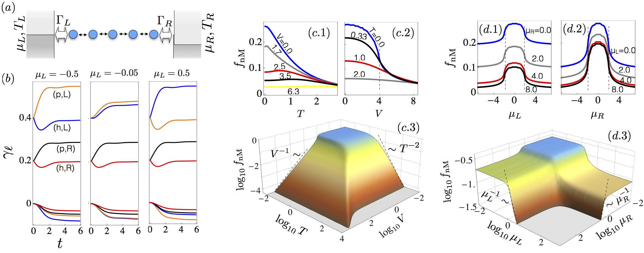
Figure 1: (a) Sketch of the system coupled to thermal reservoirs. (b) Decoherence rates $\gamma_{\ell}\left(t\right)$ as a function of time computed for $M=50,\Gamma_{L}=0.4$, $\Gamma_{R}=0.2,$ $T=0$, and $\mu_{R}=0.5$ for different values of $\mu_{L}$. The labels (p/h,L/R) refer to the particle or hole nature of the single-particle state $\left|\ell\left(t\right)\right\rangle$ and to its localization with respect to the boundary. Negative eigenvalues with the same labels as their positive counterparts are depicted in the same line-color. (c) Measure of non-Markovianity $f_{\text{nM}}$ for the steady-state process computed for $M=50,\Gamma_{L}=0.6$, $\Gamma_{R}=0.2,$ $T_{L}=T_{R}=T$ and $\mu_{L}=-\mu_{R}=V/2$ as a function of $T$ and $V$. (d) The same as in (c) for $T_{L}=T_{R}=0$ as a function of $\mu_{L}$ and $\mu_{R}$.

Open quadratic models

Consider a generic quadratic fermionic system coupled to non-interacting fermionic reservoirs (leads) labeled by $\nu=1,...,m$. The fermionic operators of the system and of the reservoirs are denoted $c_{a=1,...,n}$ and $f_{\nu_{a=1,2,...}}$, respectively. The total Hamiltonian is given by $H=H_{c}+\sum_{\nu}H_{\nu}+H_{c-\nu}$ where $H_{c}=\frac{1}{2}\boldsymbol{C}^{\dagger}\boldsymbol{H}_{c}\boldsymbol{C}$ is the Hamiltonian of the system, with $\boldsymbol{H}_{c}$ the single particle Hamiltonian and $\boldsymbol{C}=\left\{c_{1},...,c_{n},c_{1}^{\dagger},....,c_{n}^{\dagger}\right\}^{T}$ the Nambu vector. $H_{\nu}=\sum_{i}\varepsilon_{\nu}\left(f_{\nu_{i}}^{\dagger}f_{\nu_{i}}-\frac{1}{2}\right)$ is the Hamiltonian of the $\nu$-th reservoir. The interaction Hamiltonian is given by $H_{c-\nu}=\frac{1}{2}\sum_{\nu}\left(\boldsymbol{F}_{\nu}^{\dagger}\boldsymbol{T}_{\nu}^{\dagger}\boldsymbol{C}+\boldsymbol{C}^{\dagger}\boldsymbol{T}_{\nu}\boldsymbol{F}_{\nu}\right)$ with $\boldsymbol{F}_{\nu}=\left\{f_{\nu_{1}},...,f_{\nu_{n_{\nu}}},f_{\nu_{1}}^{\dagger},...,f_{\nu_{n_{\nu}}}^{\dagger}\right\}^{T}$ and $\boldsymbol{T}_{\nu}$ the hopping matrix explicitly given by $\boldsymbol{T}_{\nu}=\sum_{l}\left(t{}_{\nu_{l}}\left|\nu_{l}\right\rangle\left\langle\Omega_{\nu_{l}}\right|-\bar{t}_{\nu_{l}}\left|\hat{\nu_{l}}\right\rangle\left\langle\hat{\Omega}_{\nu_{l}}\right|\right)$ where $\left|\nu_{l}\right\rangle$ is a single-particle state of the system, coupled to the reservoir $\nu$, $\left|\Omega_{\nu_{l=1,2,...}}\right\rangle=\sum_{\varepsilon_{\nu}}\,\Omega_{\nu_{l}}\left(\varepsilon_{\nu}\right)\left|\varepsilon_{\nu}\right\rangle$ are single-particle states of the reservoir $\nu$ and $t{}_{\nu_{l}}$ is the hopping amplitude. $\left|\hat{\nu_{l}}\right\rangle$ and $\left\langle\hat{\Omega}_{\nu_{l}}\right|$ denote the particle-hole transformed of $\left|\nu_{l}\right\rangle$ and $\left\langle\Omega_{\nu_{l}}\right|$.

After the coupling is turned on at $t=0$, we consider the joint system-reservoir evolution, taken to be initially in a product state. Each reservoir, being a macroscopic system, has its initial state specified by $\beta_{\nu}$, the inverse temperature, and $\mu_{\nu}$, the chemical potential. The initial density matrix of the system is taken to be of the generic quadratic form $\rho\left(0\right)=e^{-\frac{1}{2}\boldsymbol{C}^{\dagger}\boldsymbol{\Omega}_{0}\boldsymbol{C}}/Z$ with $\boldsymbol{\Omega}_{0}$ a single-particle operator.

The Dyson equation on the Keldysh contour is derived by standard non-equilibrium Green’s functions techniques Kamenev (2011) (the derivation is sketched in the supplementary material for completeness). At this point we make a crucial assumption respecting the environment properties - the so called wide-band limit - which amounts to say that the density of states $\rho_{\nu}\left(\varepsilon\right)=\sum_{\varepsilon_{\nu}}\delta\left(\varepsilon-\varepsilon_{\nu}\right)$ of the reservoirs and the amplitudes $\Omega_{\nu_{l}}\left(\varepsilon_{\nu}\right)$ are essentially constant with respect to the energy scales of the system, i.e. $\rho_{\nu}\left(\varepsilon\right)\simeq\rho_{\nu}$, $\Omega_{\nu_{l}}\left(\varepsilon_{\nu}\right)\simeq\Omega_{\nu_{l}}$. Denoting $\boldsymbol{g}_{\nu}^{R/A/K}\left(\omega\right)$, the retarded, advanced and Keldysh components of the bare Greens Function of the reservoirs, the wide-band limit translates to $\left\langle\Omega_{\nu_{l}}\right|\boldsymbol{g}_{\nu}^{R/A}\left(\omega\right)\left|\Omega_{\nu_{l^{\prime}}}\right\rangle\simeq\mp i\pi\rho_{\nu}\bar{\Omega}_{\nu_{l}}\Omega_{\nu_{l^{\prime}}}$ and $\left\langle\Omega_{\nu_{l}}\right|\boldsymbol{g}_{\nu}^{K}\left(\omega\right)\left|\Omega_{\nu_{l^{\prime}}}\right\rangle\simeq-2\pi i\rho_{\nu}\bar{\Omega}_{\nu_{l}}\Omega_{\nu_{l^{\prime}}}\tanh\left[\beta_{\nu}\left(\omega-\mu_{\nu}\right)\right]$. In this limit, the self-energy components are $\boldsymbol{\Sigma}_{c}^{R/A}(t,t^{\prime})=\mp i\sum_{\nu}\left(\boldsymbol{\Gamma}_{\nu}+\hat{\boldsymbol{\Gamma}}_{\nu}\right)\delta\left(t-t^{\prime}\right)$ and $\boldsymbol{\Sigma}_{c}^{K}\left(t,t^{\prime}\right)=-2i\sum_{\nu}\left[\boldsymbol{\Gamma}_{\nu}F_{\nu}\left(t-t^{\prime}\right)-\hat{\boldsymbol{\Gamma}}_{\nu}\bar{F}_{\nu}\left(t-t^{\prime}\right)\right]$, where $F_{\nu}\left(t\right)=\int\frac{d\varepsilon}{2\pi}\tanh\left[\beta_{\nu}\left(\varepsilon-\mu_{\nu}\right)\right]e^{-i\varepsilon t}$, $\boldsymbol{\Gamma}_{\nu}=\sum_{ll^{\prime}}\pi\rho_{\nu}\bar{\Omega}_{\nu_{l}}\Omega_{\nu_{l^{\prime}}}t_{\nu_{l}}\bar{t}_{\nu_{l^{\prime}}}\left|\nu_{l}\right\rangle\left\langle\nu_{l^{\prime}}\right|$ . A different set of assumptions leading to a similar $\boldsymbol{\Sigma}_{c}^{R/A}$ was used in Dhar et al. (2012) to study steady-state transport. The retarded and advanced Green’s functions are given by $\boldsymbol{G}_{c}^{R}\left(t,t^{\prime}\right)=-i\Theta\left(t-t^{\prime}\right)e^{-i\left(t-t^{\prime}\right)\boldsymbol{K}},$ and $\boldsymbol{G}_{c}^{A}\left(t,t^{\prime}\right)=\boldsymbol{G}_{c}^{R}\left(t^{\prime},t\right)^{\dagger}$, where $\boldsymbol{K}=\boldsymbol{H}_{c}-i\boldsymbol{\Gamma}$ and $\boldsymbol{\Gamma}=\sum_{\nu}\left(\boldsymbol{\Gamma}_{\nu}+\hat{\boldsymbol{\Gamma}}_{\nu}\right)$. The Keldysh component is given by $\boldsymbol{G}_{c}^{K}\left(t,t^{\prime}\right)=e^{-it\boldsymbol{K}}\boldsymbol{G}_{c}^{K}\left(0,0\right)e^{it^{\prime}\boldsymbol{K}^{\dagger}}+\int_{0}^{t}dt_{1}\int_{0}^{t^{\prime}}dt_{2}e^{-i\left(t-t_{1}\right)\boldsymbol{K}}\boldsymbol{\Sigma}_{c}^{K}\left(t_{1},t_{2}\right)e^{-i\left(t_{2}-t^{\prime}\right)\boldsymbol{K}^{\dagger}}$ where $\boldsymbol{G}_{c}^{K}\left(0,0\right)=-i\tanh\left(\boldsymbol{\Omega}_{0}\right)$ is determined by the initial condition of the system.

Master equation

Under the evolution given by Eq.(1), for a quadratic Hamiltonian and linear jump operators $L_{\ell}\left(t\right)=\sum_{i}\left\langle\ell\left(t\right)\right.\left|i\right\rangle C_{i}$ (with $\left\langle\ell\left(t\right)\right.\left|\ell^{\prime}\left(t\right)\right\rangle=\delta_{\ell,\ell^{\prime}}$), an initial Gaussian density matrix remains of the Gaussian form: $\rho\left(t\right)=e^{-\frac{1}{2}\boldsymbol{C}^{\dagger}\boldsymbol{\Omega}\left(t\right)\boldsymbol{C}}/Z\left(t\right)$ and the single-particle correlation matrix, given by $\boldsymbol{\chi}\left(t\right)=\left\langle\boldsymbol{C}\left(t\right).\boldsymbol{C}^{\dagger}\left(t\right)\right\rangle=\left[1+e^{-\boldsymbol{\Omega}\left(t\right)}\right]^{-1}$, fully encodes all the equal-time properties of the system. Under the Lindblad dynamics $\boldsymbol{\chi}\left(t\right)$ evolves as (see Prosen (2008) and supplementary material for a derivation):

$$\partial_{t}\boldsymbol{\chi}\left(t\right) = -i\boldsymbol{Q}\left(t\right)\boldsymbol{\chi}\left(t\right)+i\boldsymbol{\chi}\left(t\right)\boldsymbol{Q}^{\dagger}\left(t\right)+\boldsymbol{N}\left(t\right)$$ (2)

with $\boldsymbol{N}\left(t\right)=\sum_{\ell}\gamma_{\ell}\left(t\right)\left|\ell\left(t\right)\right\rangle\left\langle\ell\left(t\right)\right|$ and $\boldsymbol{Q}\left(t\right)=\boldsymbol{H}_{c}\left(t\right)-i\frac{1}{2}\left[\boldsymbol{N}\left(t\right)+\hat{\boldsymbol{N}}\left(t\right)\right]$. Using $\boldsymbol{\chi}\left(t\right)=\frac{1}{2}\left[i\boldsymbol{G}_{c}^{K}\left(t,t\right)+1\right]$ and deriving in order to $t$, we can identify the different elements of Eq.(2):

$$\boldsymbol{Q}\left(t\right)=\boldsymbol{K}; \boldsymbol{N}\left(t\right)=\sum_{\nu}\boldsymbol{N}_{\nu}\left(t\right)$$ (3)

with

$$\boldsymbol{N}_{\nu}\left(t\right)=\left(\boldsymbol{\Gamma}_{\nu}+\hat{\boldsymbol{\Gamma}}_{\nu}\right)\\ +i\left\{R\left[\left(\boldsymbol{K}+\mu_{\nu}\right),\beta_{\nu},t\right]\boldsymbol{\Gamma}_{\nu}-\boldsymbol{\Gamma}_{\nu}R\left[\left(\boldsymbol{K}+\mu_{\nu}\right),\beta_{\nu},t\right]^{\dagger}\right.\\ \left.+R\left[\left(\boldsymbol{K}-\mu_{\nu}\right),\beta_{\nu},t\right]\hat{\boldsymbol{\Gamma}}_{\nu}-\hat{\boldsymbol{\Gamma}}_{\nu}R\left[\left(\boldsymbol{K}-\mu_{\nu}\right),\beta_{\nu},t\right]^{\dagger}\right\}$$ (4)

where $R\left[\omega,\beta,t\right]=s\left[\beta\omega,t/\beta\right]+r\left[\omega t\right]$, with $s\left[z,\tau\right]=-\int_{0}^{\tau}d\tau^{\prime}\,e^{-iz\tau^{\prime}}\int_{0}^{\infty}dx\left(\tanh\left[x\right]-1\right)\sin\left(x\tau^{\prime}\right)/\pi$ and $r\left[x\right]=\left[\log\left(ix\right)+\Gamma\left(0,ix\right)+\gamma+\log\left(\frac{4}{\pi}\right)\right]/\pi$, are obtained by a suitable regularization of the wide-band limit (see supplementary material).

The decoherence rates $\gamma_{\ell}\left(t\right)$ and the vectors $\left|\ell\left(t\right)\right\rangle$, characterizing the jump operators, can be obtained by diagonalizing $\boldsymbol{N}\left(t\right)$. Eqs. (3) show explicitly how to obtain the master equation describing a non-Markovian process and are the central result of this letter. The more general case where the system Hamiltonian and the system-environment couplings depend on time is straitforwardly obtained and is given in the supplementary material.

Particularly simple cases yielding to the Markovian dynamics arise for fully empty or fully filled reservoirs Gurvitz and Prager (1996); Gurvitz (1998), i.e. $\mu_{\nu}\to\pm\infty$, for which $\boldsymbol{N}_{\nu}\left(t\right)=2\hat{\boldsymbol{\Gamma}}_{\nu}$ and $\boldsymbol{N}_{\nu}\left(t\right)=2\boldsymbol{\Gamma}_{\nu}$ respectively, and for the infinite temperature, $\beta_{\nu}\to 0$, for which $\boldsymbol{N}_{\nu}\left(t\right)=\boldsymbol{\Gamma}_{\nu}+\hat{\boldsymbol{\Gamma}}_{\nu}$.

In the asymptotic long time limit $\boldsymbol{N}\left(t\right)$ converges to a time-independent matrix $\boldsymbol{N}_{\infty}$. If a unique steady-state exists, the single particle density matrix is given by $\boldsymbol{\chi}_{\infty}=-i\sum_{\beta\gamma}\left|\beta\right\rangle\frac{\left\langle\beta^{\prime}\right|\boldsymbol{N}_{\infty}\left|\gamma^{\prime}\right\rangle}{\lambda_{\beta}-\bar{\lambda}_{\gamma}}\left\langle\gamma\right|$ where $\left|\beta\right\rangle$ and $\left\langle\beta^{\prime}\right|$ are right and left eigenvectors of $\boldsymbol{K}$ with eigenvalue $\lambda_{\beta}$ and $\left\langle\gamma\right.\left|\beta^{\prime}\right\rangle=\delta_{\gamma\beta}$.

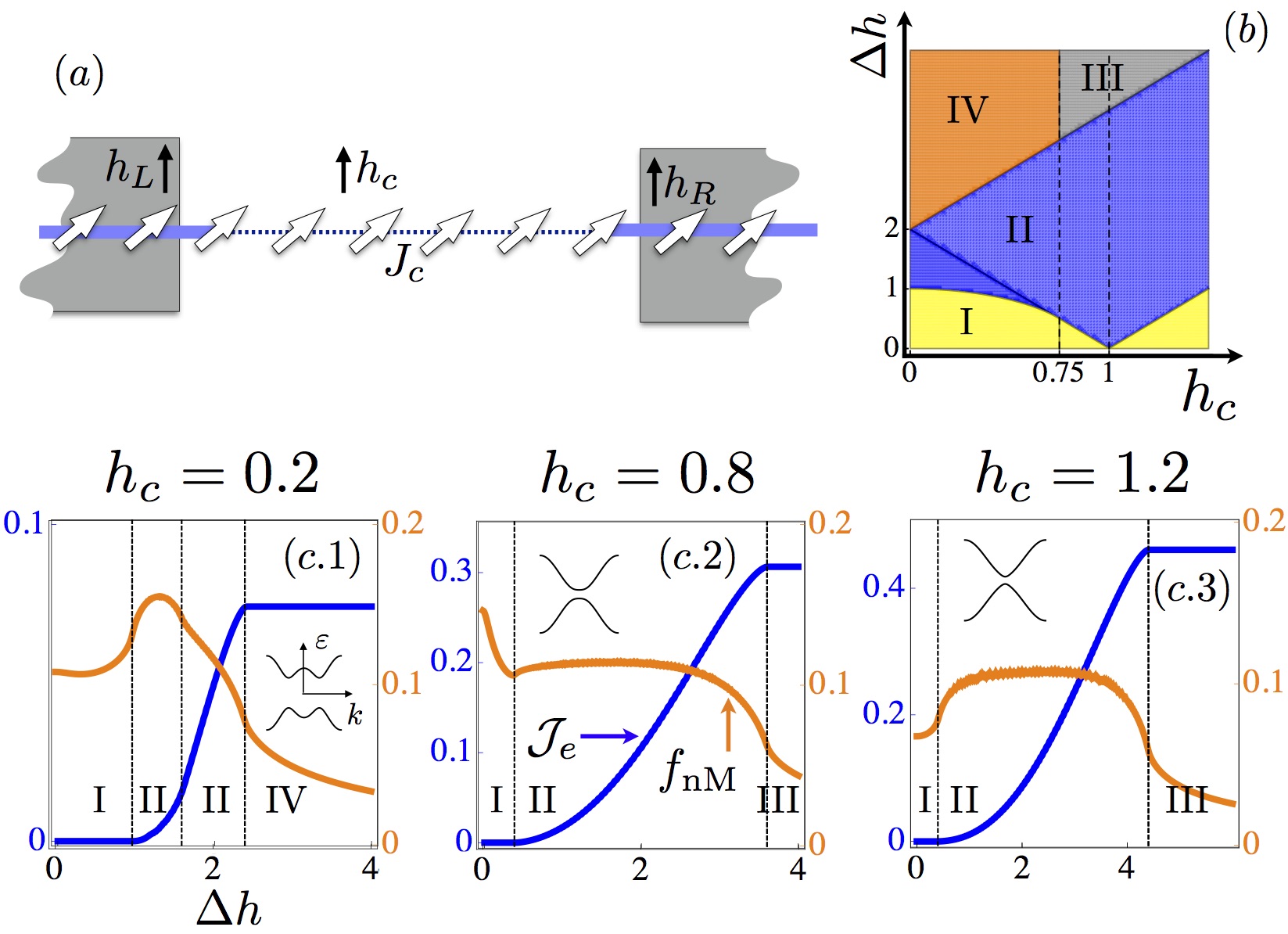
Figure 2: (a) Sketch of the XY model coupled to spin reservoirs with $T_{L}=T_{R}=0$ and $h_{L}=-h_{R}=\Delta h$. (b) Phase diagram of the non-equilibrium steady-state in the $h_{c}-\mathbf{\Delta}h$ plane computed for $\gamma_{c}=0.5$, $J_{c}=1$. Regions I to IV are described in the text. (c) Measure of non-Markovianity $f_{\text{nM}}$ and energy current $\mathcal{J}_{e}$ as a function of the spin unbalance $\Delta h$ computed for different values of $h_{c}$ and $\gamma_{c}=0.5$. The band-structure of the spin-less Jordan-Wigner fermions are depicted in the insets.

Tight-binding chain

In order to demonstrate our approach let us consider a tight-binding one-dimensional chain in Fig.1-(a), with $\boldsymbol{H}_{c}=\text{diag}\left(\boldsymbol{h},-\boldsymbol{h}^{T}\right)$ and $\boldsymbol{h}=-\sum_{j=0}^{M-2}\left|j\right\rangle\left\langle j+1\right|+\left|j+1\right\rangle\left\langle j\right|$, coupled to two leads at positions $0$ and $M-1$ by the hybridization operators $\boldsymbol{\Gamma}_{L}=\Gamma_{L}\left|0\right\rangle\left\langle 0\right|$ and $\boldsymbol{\Gamma}_{R}=\Gamma_{R}\left|M-1\right\rangle\left\langle M-1\right|$.

Fig.1-(b) shows the evolution of the decoherence rates $\gamma_{\ell}\left(t\right)$, after the coupling to the reservoirs has been turned on, for different values of $\mu_{L}$. There are 8 non-zero eigenvalues of $\boldsymbol{N}$, arising in positive-negative pairs (see code color). In the Markovian limit the negative eigenvalues tend to zero. The labels p/h refer to the particle or hole nature of the corresponding eigenvector of $\boldsymbol{N}$, and L/R to their localization near the left or right lead. For $M\to\infty$ we observe that $\boldsymbol{N}_{R/L}\left|\ell_{L/R}\left(t\right)\right\rangle\to 0$, where $\boldsymbol{N}_{\nu}\left(t\right)\left|\ell_{\nu}\left(t\right)\right\rangle=\gamma_{\ell;\nu}\left(t\right)\left|\ell_{\nu}\left(t\right)\right\rangle$, i.e. for a large size chain the contribution of both reservoirs factorizes and the non-zero eigenvalues of $\boldsymbol{N}$ can be obtained by direct sum of the spectrum of $\boldsymbol{N}_{L}$ and $\boldsymbol{N}_{R}$. This factorization explains that in Fig.1-(b) the R-labeled eigenvalues are unaffected by changes in $\mu_{L}$. More generally, such a factorization, arising when the special separation between the reservoirs is large, is to be expected for short-range Hamiltonians $H_{c}$ and allows to treat the decoherence rates of each reservoir independently. In the present example the structure of $\boldsymbol{N}_{\nu}$ is particularly simple: $\boldsymbol{N}_{\nu}\left(t\right)=\left|y_{\nu}^{p}\left(t\right)\right\rangle\left\langle\nu\right|+\left|\nu\right\rangle\left\langle y_{\nu}^{p}\left(t\right)\right|+\left|y_{\nu}^{h}\left(t\right)\right\rangle\left\langle\hat{\nu}\right|+\left|\hat{\nu}\right\rangle\left\langle y_{\nu}^{h}\left(t\right)\right|$ with $\left|y_{\nu}^{p}\left(t\right)\right\rangle=\left\{\frac{1}{2}+iR\left[\left(\boldsymbol{K}+\mu_{\nu}\right),\beta_{\nu},t\right]\right\}\boldsymbol{\Gamma}_{\nu}\left|\nu\right\rangle$ and $\left|y_{\nu}^{h}\left(t\right)\right\rangle=\left\{\frac{1}{2}+iR\left[\left(\boldsymbol{K}-\mu_{\nu}\right),\beta_{\nu},t\right]\right\}\hat{\boldsymbol{\Gamma}}_{\nu}\left|\hat{\nu}\right\rangle$; yielding to $\gamma_{\left(p,\nu\right)}^{\pm}=\frac{1}{2}\left\{\left\langle\nu\right.\left|y_{\nu}^{p}\right\rangle+\frac{1}{2}\left\langle y_{\nu}^{p}\right.\left|\nu\right\rangle\right.\pm\left(\left(\left\langle\nu\right.\left|y_{\nu}^{p}\right\rangle+\left\langle y_{\nu}^{p}\right.\left|\nu\right\rangle\right)^{2}\right.+\left.\left.4\left(\left\langle y_{\nu}^{p}\right.\left|y_{\nu}^{p}\right\rangle-\left\langle\nu\right.\left|y_{\nu}^{p}\right\rangle\left\langle y_{\nu}^{p}\right.\left|\nu\right\rangle\right)\right)^{1/2}\right\}$ and to a similar expression for their hole counterparts, corresponding to the two positive and negative eigenvalue pairs in Fig.1-(b). Note that $\gamma_{\left(p,\nu\right)}^{-}$ is zero only (Markovian case) if $\left|y_{\nu}^{p}\right\rangle\propto\left|\nu\right\rangle$. The fact that in Fig.1-(b) the particle or hole nature of the L-labeled eigenvalues is interchanged upon switching $\mu_{L}\to-\mu_{L}$ can be seen in the expressions of $\left|y_{\nu}^{p/h}\right\rangle$ together with the fact that $\boldsymbol{K}$ has no anomalous terms.

Figs.1-(c) and (d) depict the non-Markovianity nature of the steady-state as measured by the $f_{\text{nM}}=f_{\text{nM}}\left(t\to\infty\right)$. In Figs.1-(c.1,2,3) we set $\mu_{L}=-\mu_{R}=V/2$; $T_{L}=T_{R}=T$ and show $f_{\text{nM}}$ as a function of the bias voltage $V$ and temperature $T$. Figs.1-(c.1) and (c.2) show how $f_{\text{nM}}$ varies as a function of $T$ and $V$ respectively. Fig.1-(c.3) shows a logarithmic plot of $f_{\text{nM}}$ for large values of $V$ and $T$. The Markovian limit, obtained for large values $T$ or $V$, is attained differently along the two axes: $f_{\text{nM}}\propto V^{-1}$ for large $V$ and $f_{\text{nM}}\propto T^{-2}$ for large $T$.

Figs.1-(d) shows the variation of $f_{\text{nM}}$ with $\mu_{L}$ and $\mu_{R}$ separately at $T_{L}=T_{R}=0$. Fig.1-(d.3) shows clearly that the Markovian limit is attained only when both chemical potentials are large. This can be understood by the approximate factorization of the eigenvalues of $\boldsymbol{N}$ as a Markovian evolution can only arise when both reservoirs behave as memoryless environments. For $\left|\mu_{L/R}\right|\gg\left|\mu_{R/L}\right|$ one has $f_{\text{nM}}\propto\left|\mu_{L/R}\right|^{-1}$.

XY spin-chain

In the Markovian limit a number of works have addressed spin and heat transport in spin-chains Wichterich et al. (2007); Prosen and Pižorn (2008); Prosen and Žunkovič (2010); Vogl et al. (2012); Cai and Barthel (2013); Ajisaka et al. (2014). Here, we consider a XY spin-chain with non-Markovian reservoirs, depicted in Fig.2-(a). The Hamiltonian is given by $H=-\sum_{m}\frac{J}{2}\left[\left(1+\gamma\right)\sigma_{m}^{x}\sigma_{m+1}^{x}\right.+\left.\left(1-\gamma\right)\sigma_{m}^{y}\sigma_{m+1}^{y}\right]-h\sum_{m}\sigma_{m}^{z},$ where $J=J_{c}$, $\gamma=\gamma_{c}$ and $h=h_{c}$ within the central region. Setting $J=J_{L/R}$ with $J_{L/R}/J_{c}\gg 1$ and $\gamma=0$, the side chains act as wide-band gapless reservoirs with $h=h_{L/R}$. In the following we set $h_{L}=-h_{R}=\Delta h$ and work in units where $J_{c}=1$. The coupling Hamiltonian is given by $H_{int}=-\frac{J^{\prime}_{L}}{2}\left[\sigma_{L,0}^{x}\sigma_{0}^{x}+\sigma_{L,0}^{y}\sigma_{0}^{y}\right]-\frac{J^{\prime}_{R}}{2}\left[\sigma_{R,0}^{x}\sigma_{M-1}^{x}+\sigma_{R,0}^{y}\sigma_{M-1}^{y}\right]$. Employing a Jordan-Wigner mapping this model can be transformed into a set of non-interacting spineless fermions. For the central region one has $\boldsymbol{H}_{c}=\left(\begin{array}[]{cc}\boldsymbol{h}&\boldsymbol{\Delta}\\ \boldsymbol{\Delta}^{\dagger}&\boldsymbol{-h}^{T}\end{array}\right)$ with $\boldsymbol{h}=-J_{c}\sum_{j=0}^{M-2}(\left|m\right\rangle\left\langle m+1\right|+\left|m+1\right\rangle\left\langle m\right|)-2h_{c}\sum_{m=0}^{M-1}\left|m\right\rangle\left\langle m\right|$ and $\boldsymbol{\Delta}=J_{c}\gamma_{c}\sum_{j=0}^{M-2}\left[\left|m\right\rangle\left\langle\hat{m+1}\right|-\left|m+1\right\rangle\left\langle\hat{m}\right|\right]$. Following our wide-band treatment for the reservoirs (i.e. $J_{L/R}/J_{c}\to\infty$) we obtain $\boldsymbol{\Gamma}_{L}=\Gamma_{L}\left|0\right\rangle\left\langle 0\right|$ and $\boldsymbol{\Gamma}_{R}=\Gamma_{R}\left|M-1\right\rangle\left\langle M-1\right|$, where $\Gamma_{L/R}\propto J^{\prime 2}/J_{L/R}$ are constants that characterize the contacts, and $\mu_{L/R}=2h_{L/R}$.

In the Markovian limit ($\Delta h\to\infty$) this model was shown to exhibit a steady-state phase transition, where the decay of the correlators $C_{l,m}=\left\langle\sigma_{l}^{z}\sigma_{m}^{z}\right\rangle-\left\langle\sigma_{l}^{z}\right\rangle\left\langle\sigma_{m}^{z}\right\rangle$, as a function of $r=\left|l-m\right|$, passes from power law (for $h_{c}/J_{c}<1-\gamma_{c}^{2}$) to exponential (for $h_{c}/J_{c}>1-\gamma_{c}^{2}$) Prosen and Pižorn (2008). We address the non-Markovian regime (finite $\Delta h$) and monitor the steady-state energy-current $\mathcal{J}_{e}$ and $f_{\text{nM}}$ in addition to $C_{l,m}$ (the explicit forms of $\mathcal{J}_{e}$ and $C_{l,m}$ are given in the supplementary material). Fig.2-(b) shows the phase diagram in the $h_{c}-\Delta h$ plane and signals the four different steady-state phases. The energy current and $f_{\text{nM}}$ as a function of $\Delta h$ are given in Figs.2-(c.1-3) for different values of $h_{c}.$ A numerical demonstration of the exponential/algebraic decay of $C_{l,m}$ within each region is provided in the supplementary material. In region I both effective chemical potentials ($\mu_{L/R}$) are below the excitation-gap. This region shows a vanishing energy current and an exponential decay of $C_{l,m}$. In region II there is energy transport with a finite $d\mathcal{J}_{e}/d\Delta h$ and an algebraic decay of $C_{l,m}$. In this region $\mu_{R/L}$ lay within the excitation energy band. Region III and IV show a saturation of the energy current and $f_{\text{nM}}$ behaves as $1/\Delta h$ as the Markovian limit is taken. However, in III, $C_{l,m}$ is algebraically decaying whereas is IV the decay is exponential.

These results show that the two Markovian phases reported in Prosen and Pižorn (2008) can be continuously connected to phases III and IV. Moreover deep into the non-Markovian regime phases I and II arise having no non-Markovian analog.

Discussion

We provide an explicit construction of the master equations for quadratic fermionic models coupled to wide-band reservoirs by identifying the jump operators and the decoherence rates derived with the non-equilibrium Green’s functions formalism. This approach permits to study non-Markovian regimes characterized by negative decoherence rates and to clarify the regimes where the Markovian approximation yields a good approximation for the dynamics. We illustrate our findings with two examples of non-Markonian evolution. The XY model shows a particularly rich set of phases with distinct physical properties.

Our results provide an explicit approach to study real-time dynamics of a wide class of open systems. As quadratic models are often used as starting points of perturbative and variational approaches, our results might also be of interest to study master-equations of interacting models.

Supplementary Material

Appendix A Preliminary considerations

A.1 Notation

For a generic fermionic system with $n$ modes, obeying the anti-commutation relations $\left\{c_{a},c_{b}^{\dagger}\right\}=\delta_{a,b};\,\left\{c_{a},c_{b}\right\}=\left\{c_{a}^{\dagger},c_{b}^{\dagger}\right\}=0$, $\left(a,b=1,...,n\right)$, we define $\boldsymbol{C}=\left\{c_{1},...,c_{n},c_{1}^{\dagger},....,c_{n}^{\dagger}\right\}^{T}$ as the column vector of annihilation and creation operators. For definiteness we take the indices $a$ and $b$ as labeling the position of a fermion on a finite lattice, such that $\left|a\right\rangle$ ($\left|\hat{a}\right\rangle$ ) corresponds to a particle (hole) at position $a$. The indices $i,j$ are used to label all single-particle or hole states $\left|i\right\rangle\in\left\{\left|a\right\rangle\right\}\cup\left\{\left|\hat{a}\right\rangle\right\}$. With these definitions one has $\left\langle a\right|\boldsymbol{C}=c_{a}$, $\left\langle\hat{a}\right|\boldsymbol{C}=c_{a}^{\dagger}$ or equivalently $\left\langle i\right|\boldsymbol{C}=\boldsymbol{C}_{i}$. In the following, the bold symbols are used for $2n\times 2n$ matrices and $2n$ vectors. In this way a generic single-body operator $A=\sum_{a,b}(c_{a}^{\dagger}A_{a,b}^{pp}c_{a}+c_{a}A_{a,b}^{hh}c_{a}^{\dagger}+c_{a}^{\dagger}A_{a,b}^{ph}c_{b}^{\dagger}+c_{a}A_{a,b}^{hp}c_{b})$ can be written as $A=\boldsymbol{C}^{\dagger}\boldsymbol{A}\boldsymbol{C}$ with $\mathbf{A}=\sum_{a,b}(\left|a\right\rangle A_{a,b}^{pp}\left\langle b\right|+\left|a\right\rangle A_{a,b}^{ph}\left\langle\hat{b}\right|+\left|\hat{a}\right\rangle A_{a,b}^{hp}\left\langle b\right|+\left|\hat{a}\right\rangle A_{a,b}^{hh}\left\langle\hat{b}\right|)=\sum_{ij}\left|i\right\rangle\mathbf{A}_{i,j}\left\langle j\right|$ and $\text{tr}\boldsymbol{A}=0$. We define the particle-hole transform of a single-particle state $\left|\phi\right\rangle=\sum_{a}(\phi_{a}^{p}\left|a\right\rangle+\phi_{a}^{h}\left|\hat{a}\right\rangle)=\sum_{i}\phi_{i}\left|i\right\rangle$ as $\left|\hat{\phi}\right\rangle=\boldsymbol{J}\left|\phi^{*}\right\rangle$, where the conjugate $\left|\phi^{*}\right\rangle=\sum_{i}\bar{\phi}_{i}\left|i\right\rangle$ is taken with respect to the basis $\left|i\right\rangle$ and $\boldsymbol{J}=\sum_{a}\left(\left|a\right\rangle\left\langle\hat{a}\right|+\left|\hat{a}\right\rangle\left\langle a\right|\right)$ transforms single-particle (hole) states into their hole (particle) analog. A similar definition holds for the operators $\hat{\boldsymbol{A}}=\boldsymbol{J}\boldsymbol{A}^{T}\boldsymbol{J}$, with $\boldsymbol{A}^{T}=\sum_{ij}\left|i\right\rangle\mathbf{A}_{j,i}\left\langle j\right|$.

A.2 Green’s functions and single-body density matrix

We define the greater and lesser Green’s functions, containing both normal (i.e. $c_{a}^{\dagger}c_{b}$ and $c_{a}c_{b}^{\dagger}$ ) and anomalous (i.e. $c_{a}^{\dagger}c_{b}^{\dagger}$ and $c_{a}c_{b}$) terms, as

$$\mathbf{G}_{i,j}^{>}\left(t,t^{\prime}\right) \equiv -i\left\langle\boldsymbol{C}_{i}\left(t\right)\boldsymbol{C}_{j}^{\dagger}\left(t^{\prime}\right)\right\rangle$$ (5)

$$\mathbf{G}_{i,j}^{<}\left(t,t^{\prime}\right) \equiv i\left\langle\boldsymbol{C}_{j}^{\dagger}\left(t^{\prime}\right)\boldsymbol{C}_{i}\left(t\right)\right\rangle$$ (6)

The retarded, advanced and Keldysh Green’s functions are defined in the standard way

$$\mathbf{G}^{R}(t,t^{\prime}) \equiv \Theta(t-t^{\prime})\left[\mathbf{G}^{>}(t,t^{\prime})-\mathbf{G}^{<}(t,t^{\prime})\right]$$ (7)

$$\mathbf{G}^{A}(t,t^{\prime}) \equiv -\Theta(t^{\prime}-t)\left[\mathbf{G}^{>}(t,t^{\prime})-\mathbf{G}^{<}(t,t^{\prime})\right]$$ (8)

$$\mathbf{G}^{K}(t,t^{\prime}) \equiv \mathbf{G}^{>}(t,t^{\prime})+\mathbf{G}^{<}(t,t^{\prime})$$ (9)

The single-body correlation matrix $\boldsymbol{\chi}=\left\langle\boldsymbol{C}\boldsymbol{C}^{\dagger}\right\rangle$ can be obtained as the equal time limit of the greater Green’s function

$$\boldsymbol{\chi}_{ij}\left(t\right) = \left\langle\boldsymbol{C}_{i}\left(t\right)\boldsymbol{C}_{j}^{\dagger}\left(t\right)\right\rangle=i\boldsymbol{G}_{i,j}^{>}(t,t)$$ (10)

Noting that the greater Green’s function can be obtained as $\boldsymbol{G}^{>}=\frac{1}{2}\left[\boldsymbol{G}_{c}^{K}+\boldsymbol{G}_{c}^{R}-\boldsymbol{G}_{c}^{A}\right]$ and $\boldsymbol{G}^{R}\left(t,t\right)-\boldsymbol{G}^{A}\left(t,t\right)=-i$ this quantity is simply related to the Keldysh Green’s function

$$\boldsymbol{\chi}\left(t\right) = \frac{1}{2}\left[i\boldsymbol{G}^{K}\left(t,t\right)+1\right].$$ (11)

$\boldsymbol{\chi}\left(t\right)$ has the information about all equal time single-body correlations, for example: $\left\langle c_{a}^{\dagger}\left(t\right)c_{b}\left(t\right)\right\rangle=\left\langle\hat{a}\right|\boldsymbol{\chi}\left(t\right)\left|\hat{b}\right\rangle$. From the commutation relations among fermions and the definition of particle hole symmetry, $\boldsymbol{\chi}$ respects:

$$\boldsymbol{\chi}^{\dagger} = \boldsymbol{\chi}$$ (12)

$$\text{tr}\left(\boldsymbol{\chi}\right) = n$$ (13)

$$\hat{\boldsymbol{\chi}} = 1-\boldsymbol{\chi}$$ (14)

A.3 Closed quadratic models

A generic quadratic Hamiltonian can be written as

$$H = \frac{1}{2}\boldsymbol{C}^{\dagger}\boldsymbol{H}\boldsymbol{C}$$ (15)

where $\boldsymbol{H=}\boldsymbol{H}^{\dagger}$ is the single-body Hamiltonian given by

$$\boldsymbol{H} = \sum_{a,b}\left(\left|a\right\rangle h_{ab}\left\langle b\right|-\left|\hat{a}\right\rangle h_{ba}\left\langle\hat{b}\right|+\left|a\right\rangle\Delta_{ab}\left\langle\hat{b}\right|+\left|\hat{a}\right\rangle\bar{\Delta}_{ba}\left\langle b\right|\right)$$ (16)

where $h$ and $\Delta$ are $n\times n$ matrices with the properties $h^{\dagger}=h$ and $\Delta^{T}=-\Delta$. Note that $\boldsymbol{H}$ fulfills the particle-hole conjugation condition $\hat{\boldsymbol{H}}=-\boldsymbol{H}$ implying that if $\boldsymbol{H}\left|\varepsilon\right\rangle=\varepsilon\left|\varepsilon\right\rangle$ then $\boldsymbol{H}\left|\hat{\varepsilon}\right\rangle=-\varepsilon\left|\hat{\varepsilon}\right\rangle$.

For a non-interacting fermionic system in thermal equilibrium at $t=0$ with the Hamiltonian $H_{0}=\frac{1}{2}\boldsymbol{C}^{\dagger}\boldsymbol{H}_{0}\boldsymbol{C}$, temperature $k_{B}T=\beta^{-1}$ and chemical potential $\mu$, the density matrix is given by $\rho=e^{-\beta\left(H-\mu N\right)}/Z$ with $Z=\text{tr}\left[e^{-\beta\left(H-\mu N\right)}\right]$. Evolving the equilibrium condition under the Hamiltonian $H\left(t\right)=\frac{1}{2}\boldsymbol{C}^{\dagger}\boldsymbol{H}\left(t\right)\boldsymbol{C}$, the Green’s functions in Eq.(6) are explicitly given by

$$\mathbf{G}^{>}\left(t,t^{\prime}\right) = -i\boldsymbol{U}\left(t,0\right)\left[1-n_{f}\left(\boldsymbol{H}_{0}-\mu\boldsymbol{N}\right)\right]\boldsymbol{U}\left(0,t^{\prime}\right)$$ (17)

$$\mathbf{G}^{<}\left(t,t^{\prime}\right) = i\boldsymbol{U}\left(t,0\right)n_{f}\left(\boldsymbol{H}_{0}-\mu\boldsymbol{N}\right)\boldsymbol{U}\left(0,t^{\prime}\right)$$ (18)

where $\boldsymbol{U}\left(t,t^{\prime}\right)=Te^{-i\int_{t^{\prime}}^{t}d\tau\boldsymbol{H}\left(\tau\right)}$ is the single-body evolution operator with $T$ the time ordering operator, $n_{f}\left(z\right)=\frac{1}{e^{\beta z}+1}$ the Fermi-function and $\boldsymbol{N}=\sum_{a}\left|a\right\rangle\left\langle a\right|-\left|\hat{a}\right\rangle\left\langle\hat{a}\right|$ corresponds to the second quantized operator $N=\frac{1}{2}\boldsymbol{C}^{\dagger}\boldsymbol{N}\boldsymbol{C}+\frac{1}{2}n$ that counts the total number of particles in the system.

For the particular case of time independent Hamiltonian $H\left(t\right)=H$, the Green’s functions in Eq.(9) become

$$\mathbf{G}^{R}(t,t^{\prime}) = -i\Theta(t-t^{\prime})e^{-i\boldsymbol{H}\left(t-t^{\prime}\right)}$$ (19)

$$\mathbf{G}^{A}(t,t^{\prime}) = i\Theta(t-t^{\prime})e^{-i\boldsymbol{H}\left(t-t^{\prime}\right)}$$ (20)

$$\mathbf{G}^{K}(t,t^{\prime}) = -ie^{-i\boldsymbol{H}t}\left[1-2n_{f}\left(\boldsymbol{H}_{0}-\mu\boldsymbol{N}\right)\right]e^{i\boldsymbol{H}t^{\prime}}$$ (21)

Moreover, if $H_{0}=H$ and $H$ conserves the number of particles $\left[H,N\right]=0$, all these quantities depend on the difference of times only: $\mathbf{G}^{R,A,K}(t,t^{\prime})=\mathbf{G}^{R,A,K}(t-t^{\prime})$, and thus

$$\mathbf{G}^{R/A}(\omega) = \left(\omega-\boldsymbol{H}\pm i\eta\right)^{-1}$$ (22)

$$\mathbf{G}^{K}(\omega) = -2\pi i\left[1-2n_{f}\left(\boldsymbol{H}-\mu\boldsymbol{N}\right)\right]\delta\left(\omega-\boldsymbol{H}\right)$$ (23)

with $\mathbf{G}^{R,A,K}\left(\omega\right)=\int dt\,e^{i\omega t}\mathbf{G}^{R,A,K}\left(t\right)$.

A.4 Derivation of Dyson’s equation on the Keldysh contour

Consider the generating function on the Keldysh contour,

$$Z\left[\boldsymbol{\eta},\boldsymbol{\eta}^{\prime}\right] = \int DcDf\,e^{i\int_{\gamma}dz\,\frac{1}{2}\boldsymbol{\psi}^{\dagger}\left(z\right)\left[i\boldsymbol{\partial}_{z}-\boldsymbol{H}\right]\boldsymbol{\psi}\left(z\right)}e^{\int_{\gamma}dz\left[\boldsymbol{\eta}^{\dagger}\left(z\right).\boldsymbol{\psi}\left(z\right)+\boldsymbol{\psi}^{\dagger}\left(z\right).\boldsymbol{\eta}^{\prime}\left(z\right)\right]}$$ (24)

where $\boldsymbol{\psi}=\left(\boldsymbol{C},\boldsymbol{F}_{\nu_{1}},\boldsymbol{F}_{\nu_{2}},...\right)$, $\boldsymbol{\eta}$ and $\boldsymbol{\eta}^{\prime}$ are Grassmanian sources and where the single-particle Hamiltonian $\boldsymbol{H}$ is given by

$$\boldsymbol{H} = \left(\begin{array}[]{cccc}\boldsymbol{H}_{C}&\boldsymbol{T}_{\nu_{1}}&\boldsymbol{T}_{\nu_{2}}&\ldots\\ \boldsymbol{T}_{\nu_{1}}^{\dagger}&\boldsymbol{H}_{\nu_{1}}&0&\cdots\\ \boldsymbol{T}_{\nu_{2}}^{\dagger}&0&\boldsymbol{H}_{\nu_{2}}&\ddots\\ \vdots&\vdots&\ddots&\ddots\end{array}\right).$$ (29)

Integrating out the fermions yields to

$$\frac{Z\left[\boldsymbol{\eta},\boldsymbol{\eta}^{\prime}\right]}{Z\left[\boldsymbol{0},\boldsymbol{0}\right]} = e^{\frac{i}{2}\int_{\gamma}dzdz^{\prime}\left(\boldsymbol{\eta}^{\dagger}-\boldsymbol{\eta}^{\prime\dagger}\right)\left(z\right)\boldsymbol{G}\left(z,z^{\prime}\right)\left(\boldsymbol{\eta}^{\prime}-\boldsymbol{\eta}\right)\left(z^{\prime}\right)}$$ (30)

with

$$\boldsymbol{G} = \left(\begin{array}[]{cc}\boldsymbol{G}_{cc}&\boldsymbol{G}_{cf_{\nu}}\\ \boldsymbol{G}_{f_{\nu}c}&\boldsymbol{G}_{f_{\nu}f_{\nu^{\prime}}}\end{array}\right)$$ (33)

and

$$\boldsymbol{G}_{cc} = \left[\boldsymbol{g}_{c}^{-1}-\boldsymbol{\Sigma}_{c}\right]^{-1}$$ (34)

$$\boldsymbol{G}_{f_{\nu}c} = \boldsymbol{g}_{f_{\nu}}\boldsymbol{T}_{\nu}^{\dagger}\boldsymbol{G}_{cc}$$ (35)

$$\boldsymbol{G}_{cf_{\nu}} = \boldsymbol{G}_{cc}\boldsymbol{T}_{\nu}\boldsymbol{g}_{f_{\nu}}$$ (36)

$$\boldsymbol{G}_{f_{\nu}f_{\nu^{\prime}}} = \delta_{\nu\nu^{\prime}}\boldsymbol{g}_{f_{\nu}}+\boldsymbol{g}_{f_{\nu}}\boldsymbol{T}_{\nu}^{\dagger}\boldsymbol{G}_{cc}\boldsymbol{T}_{\nu^{\prime}}\boldsymbol{g}_{f_{\nu^{\prime}}}$$ (37)

where

$$\boldsymbol{\Sigma}_{c} = \sum_{\nu}\boldsymbol{T}_{\nu}\boldsymbol{g}_{\nu}\boldsymbol{T}_{\nu}^{\dagger}$$ (38)

Deriving both sides of Eq.(30) in order to the sources we can verify that $\left[\boldsymbol{G}_{ab}\right]_{i,j}\left(t,t^{\prime}\right)=\boldsymbol{G}_{a_{i}b_{j}}\left(t,t^{\prime}\right)$ are the path ordered Green’s function $\boldsymbol{G}_{a_{i}b_{j}}\left(t,t^{\prime}\right)=-i\left\langle T_{\gamma}a_{i}\left(t\right)b_{j}^{\dagger}\left(t^{\prime}\right)\right\rangle$ and where $T_{\gamma}$ is the path ordering operator on the Keldysh contour. $\boldsymbol{g}_{f_{\nu}}$ and $\boldsymbol{g}_{c}$ are the bare Green’s functions of lead $\nu$ and of the system respectively.

Appendix B System self-energy

B.1 Self-energy

Using the results derived for closed quadratic models, the retarded, advanced and Keldysh Green’s functions of the reservoirs, in frequency domain, are given by

$$\boldsymbol{g}_{\nu}^{R/A}\left(\omega\right) = \sum_{\varepsilon_{\nu}}\left(\left|\varepsilon_{\nu}\right\rangle\frac{1}{\omega-\varepsilon_{\nu}\pm i\eta}\left\langle\varepsilon_{\nu}\right|+\left|\hat{\varepsilon}_{\nu}\right\rangle\frac{1}{\omega+\varepsilon_{\nu}\pm i\eta}\left\langle\hat{\varepsilon}_{\nu}\right|\right)$$ (39)

$$\boldsymbol{g}_{\nu}^{K}\left(\omega\right) = -2\pi i\sum_{\varepsilon_{\nu}}F_{\nu}\left(\omega\right)\left(\left|\varepsilon_{\nu}\right\rangle\delta\left(\omega-\varepsilon_{\nu}\right)\left\langle\varepsilon_{\nu}\right|-\left|\hat{\varepsilon}_{\nu}\right\rangle\delta\left(\omega+\varepsilon_{\nu}\right)\left\langle\hat{\varepsilon}_{\nu}\right|\right)$$ (40)

with $F_{\nu}\left(\omega\right)=\left[1-2\frac{1}{e^{\beta_{\nu}\left(\omega-\mu_{\nu}\right)}+1}\right]$. Using the Langreth’s rules we can then obtain the retarded, advanced and Keldysh components of the system’s self-energy, due to the presence of the reservoirs:

$$\boldsymbol{\Sigma}_{c}^{R/A/K}(t,t^{\prime}) = \sum_{\nu,l}\left(t{}_{\nu_{l}}\bar{t}{}_{\nu_{l}^{\prime}}\left|\nu_{l}\right\rangle\left\langle\Omega_{\nu}\right|\boldsymbol{g}_{\nu}^{R/A/K}\left(t,t^{\prime}\right)\left|\Omega_{\nu}\right\rangle\left\langle\nu_{l^{\prime}}\right|\right.$$

$$\left.+\bar{t}_{\nu_{l}}t_{\nu_{l^{\prime}}}\left|\hat{\nu}_{l}\right\rangle\left\langle\hat{\Omega}_{\nu_{l}}\right|\boldsymbol{g}_{\nu}^{R/A/K}\left(t,t^{\prime}\right)\left|\hat{\Omega}_{\nu_{l^{\prime}}}\right\rangle\left\langle\nu_{l^{\prime}}\right|\right).$$

B.2 Green’s functions

B.2.1 Properties of operators

To treat the generic time dependent case, we are going to assume in this section that the system Hamiltonian $\boldsymbol{H}_{c}\left(t\right)$, the hopping amplitudes $t_{\nu_{l}}\left(t\right)$ and the single-particle states $\left|\nu_{l}\left(t\right)\right\rangle$ depend on time. In this way the matrices $\boldsymbol{\Gamma}_{\nu}$ in the main text generalize to

$$\boldsymbol{\Gamma}_{\nu}\left(t,t^{\prime}\right) = \pi\rho_{\nu}\left(0\right)\sum_{ll^{\prime}}\bar{\Omega}_{\nu_{l}}\left(0\right)\Omega_{\nu_{l^{\prime}}}\left(0\right)t_{\nu_{l}}\left(t\right)\bar{t}_{\nu_{l^{\prime}}}\left(t^{\prime}\right)\left|\nu_{l}\left(t\right)\right\rangle\left\langle\nu_{l^{\prime}}\left(t^{\prime}\right)\right|.$$ (41)

It is easy to see that:

$$\left[\boldsymbol{\Gamma}_{\nu}\left(t,t^{\prime}\right)\right]^{\dagger} = \boldsymbol{\Gamma}_{\nu}\left(t^{\prime},t\right)$$

Defining $\boldsymbol{\Gamma}\left(t\right)=\sum_{\nu}\left[\boldsymbol{\Gamma}_{\nu}\left(t,t\right)+\hat{\boldsymbol{\Gamma}}_{\nu}\left(t,t\right)\right]$ and $\boldsymbol{K}\left(t\right)=\boldsymbol{H}\left(t\right)-i\boldsymbol{\Gamma}\left(t\right)$, the particle-hole symmetric transformation yields

$$\hat{\boldsymbol{H}}\left(t\right) = -\boldsymbol{H}\left(t\right)$$

$$\hat{\boldsymbol{\Gamma}}\left(t\right) = \boldsymbol{\Gamma}\left(t\right)$$

$$\hat{\boldsymbol{K}}\left(t\right) = -\boldsymbol{K}\left(t\right)$$

B.2.2 Retarded and advanced components

Within the wide-band approximation the retarded and advanced self-energies are local in time $\boldsymbol{\Sigma}_{c}^{R/A}(t,t^{\prime})\propto\delta\left(t-t^{\prime}\right)$ and $\boldsymbol{G}_{c}^{R/A}\left(t,t^{\prime}\right)$ fulfills the differential equation

$$\left[i\partial_{t}-\boldsymbol{K}\left(t\right)\right]\boldsymbol{G}_{c}^{R}\left(t,t^{\prime}\right) = \delta\left(t-t^{\prime}\right)$$

with boundary conditions

$$\boldsymbol{G}_{c}^{R}\left(t,t^{\prime}\right) = 0\text{ for }t^{\prime}>t$$

Solving the differential equation gives

$$\boldsymbol{G}_{c}^{R}\left(t,t^{\prime}\right) = -i\Theta\left(t-t^{\prime}\right)U\left(t,t^{\prime}\right)$$

and thus

$$\boldsymbol{G}_{c}^{A}\left(t,t^{\prime}\right) = i\Theta\left(t^{\prime}-t\right)U^{\dagger}\left(t,t^{\prime}\right)$$

with

$$\boldsymbol{U}\left(t,t^{\prime}\right) = Te^{-i\int_{t^{\prime}}^{t}d\tau\boldsymbol{K}\left(\tau\right)}$$

$$\boldsymbol{U}^{\dagger}\left(t,t^{\prime}\right) \equiv \left[\boldsymbol{U}\left(t^{\prime},t\right)\right]^{\dagger}=\bar{T}e^{i\int_{t^{\prime}}^{t}d\tau\boldsymbol{K}^{\dagger}\left(\tau\right)}$$

where $T$ and $\bar{T}$ are respectively the time-ordered and anti-time-ordered operators.

B.2.3 Keldysh component

The Dyson Keldysh equations for the Keldysh component states that

$$\left[\boldsymbol{G}_{c}^{R}\right]^{-1}\boldsymbol{G}_{c}^{K} = \boldsymbol{\Sigma}_{c}^{K}\boldsymbol{G}_{c}^{A}$$ (42)

$$\boldsymbol{G}_{c}^{K}\left[\boldsymbol{G}_{c}^{A}\right]^{-1} = \boldsymbol{G}_{c}^{R}\boldsymbol{\Sigma}_{c}^{K}$$ (43)

with $\left[\boldsymbol{G}_{c}^{R}\right]^{-1}\left(t,t^{\prime}\right)=\delta\left(t,t^{\prime}\right)\left[i\partial_{t}-\boldsymbol{K}\left(t\right)\right]$ and $\left[\boldsymbol{G}_{c}^{A}\right]\left(t,t^{\prime}\right)=\left[\boldsymbol{G}_{c}^{R}\right]^{\dagger}\left(t^{\prime},t\right)$. In integral form we have

$$i\partial_{t}\boldsymbol{G}_{c}^{K}\left(t,t^{\prime}\right) = \boldsymbol{K}\left(t\right)\boldsymbol{G}_{c}^{K}\left(t,t^{\prime}\right)+i\int_{0}^{t}d\tau\,\boldsymbol{\Sigma}_{c}^{K}\left(t,\tau\right)U^{\dagger}\left(\tau,t^{\prime}\right)$$ (44)

$$-i\partial_{t^{\prime}}\boldsymbol{G}_{c}^{K}\left(t,t^{\prime}\right) = \boldsymbol{G}_{c}^{K}\left(t,t^{\prime}\right)\boldsymbol{K}^{\dagger}\left(t^{\prime}\right)-i\int_{0}^{t}d\tau\,U\left(t,\tau\right)\boldsymbol{\Sigma}_{c}^{K}\left(\tau,t^{\prime}\right)$$ (45)

The solution of these integral differential equations is given by

$$\boldsymbol{G}_{c}^{K}\left(t,t^{\prime}\right) = U\left(t,0\right)\boldsymbol{G}_{c}^{K}\left(0,0\right)U^{\dagger}\left(0,t^{\prime}\right)+\int_{0}^{t}dt_{1}\int_{0}^{t^{\prime}}dt_{2}U\left(t,t_{1}\right)\boldsymbol{\Sigma}_{c}^{K}\left(t_{1},t_{2}\right)U^{\dagger}\left(t_{2},t^{\prime}\right)$$ (46)

where $\boldsymbol{G}_{c}^{K}\left(0,0\right)$ is the initial condition that depends on the initial density matrix of the system.

Appendix C Quadratic Lindblad operators

C.0.1 Adjoint Lindblad equation

The Lindblad equation for the evolution of the density matrix is given by

$$\partial_{\tau}\rho\left(t\right) = \mathcal{L}\left[\rho\left(t\right)\right]$$ (47)

$$\mathcal{L}\left[\rho\right] = \mathcal{L}_{0}\left[\rho\right]+\sum_{\mu\neq 0}\mathcal{L}_{\mu}\left[\rho\right]$$ (48)

$$\mathcal{L}_{0}\left[\rho\right] = -i\left[H,\rho\right]$$ (49)

$$\mathcal{L}_{\mu}\left[\rho\right] = \gamma_{\mu}\left(2L_{\mu}\rho L_{\mu}^{\dagger}-\left\{L_{\mu}^{\dagger}L_{\mu},\rho\right\}\right)$$ (50)

where $H$ is the Hamiltonian of the system and $L_{\mu}$’s are due to the interaction with the environment.

Given the mean value of an observable $\mathcal{O}\left(t\right)=\text{tr}\left[O\rho\left(t\right)\right]$ we define $\mathcal{L}^{\text{ad}}$ such that

$$\partial_{t}\mathcal{O}\left(t\right) = \text{tr}\left\{O\mathcal{L}\left[\rho\left(t\right)\right]\right\}$$ (51)

$$= \text{tr}\left\{\mathcal{L}^{\text{ad}}\left[O\right]\rho\left(t\right)\right\}$$ (52)

were we find by invariance of the trace

$$\mathcal{L}^{\text{ad}}\left[O\right] = \mathcal{L}_{0}^{\text{ad}}\left[O\right]+\sum_{\mu\neq 0}\mathcal{L}_{\mu}^{\text{ad}}\left[O\right]$$ (53)

$$\mathcal{L}_{0}^{\text{ad}}\left[O\right] = i\left[H,O\right]$$ (54)

$$\mathcal{L}_{\mu}^{\text{ad}}\left[O\right] = \gamma_{\mu}\left\{L_{\mu}^{\dagger}\left[O,L_{\mu}\right]+\left[L_{\mu}^{\dagger},O\right]L_{\mu}\right\}$$ (55)

This means that the mean values of operators can be computed also in the adjoint representation with

$$\mathcal{O}\left(t\right) = \text{tr}\left[O\rho\left(t\right)\right]=\text{tr}\left[O\left(t\right)\rho(0)\right]$$ (56)

$$\partial_{t}O\left(t\right) = \mathcal{L}^{\text{ad}}\left[O\left(t\right)\right]$$ (57)

which is the analog of the Heisenberg representation in usual Hamiltonian dynamics.

C.0.2 Lindblad equation for $\boldsymbol{\chi}\left(t\right)$

For $H=\frac{1}{2}\boldsymbol{C}^{\dagger}.\boldsymbol{H}_{c}.\boldsymbol{C}$ and $L_{\ell}\left(t\right)=\sum_{i}\left\langle\ell\left(t\right)\right.\left|i\right\rangle C_{i}$, one obtains, using the fermionic commutation relations,

$$\mathcal{L}_{0}^{\text{ad}}\left[\boldsymbol{C}\boldsymbol{C}^{\dagger}\right] = -i\left(\boldsymbol{H}_{c}\boldsymbol{C}\boldsymbol{C}^{\dagger}-\boldsymbol{C}\boldsymbol{C}^{\dagger}\boldsymbol{H}_{c}\right)$$ (58)

$$\sum_{\mu\neq 0}\mathcal{L}_{\mu}^{\text{ad}}\left[\boldsymbol{C}\boldsymbol{C}^{\dagger}\right] = -\boldsymbol{M}\boldsymbol{C}\boldsymbol{C}^{\dagger}-\boldsymbol{C}\boldsymbol{C}^{\dagger}\boldsymbol{M}+\boldsymbol{N}$$ (59)

with

$$\boldsymbol{M} = \frac{1}{2}\left(\boldsymbol{N}+\boldsymbol{J}.\boldsymbol{N}^{*}.\boldsymbol{J}\right),$$ (60)

$$\boldsymbol{N} = \sum_{\mu}\left|\ell_{\mu}\right\rangle\gamma_{\mu}\left\langle\ell_{\mu}\right|.$$ (61)

With the above expressions and for time dependent $\boldsymbol{H}_{c}$ and $\boldsymbol{N}$ the evolution of the one body-density matrix: $\partial_{t}\boldsymbol{\chi}\left(t\right)=\text{tr}\left\{\mathcal{L}^{\text{ad}}\left[\left(\boldsymbol{C}\boldsymbol{C}^{\dagger}\right)(t)\right]\rho_{0}\right\}$, can be written as

$$\partial_{t}\boldsymbol{\chi}\left(t\right) = -i\boldsymbol{Q}\left(t\right)\boldsymbol{\chi}\left(t\right)+i\boldsymbol{\chi}\left(t\right)\boldsymbol{Q}^{\dagger}\left(t\right)+\boldsymbol{N}\left(t\right)$$ (62)

with $\boldsymbol{Q}=\boldsymbol{H}_{c}-i\boldsymbol{M}$. This equation should be compared with Eqs.(44, 45). It can be integrated similarly to Eq.(46) yielding to

$$\boldsymbol{\chi}\left(t\right) = U\left(t,0\right)\boldsymbol{\chi}\left(0\right)U^{\dagger}\left(0,t\right)+\int_{0}^{t}dt^{\prime}U\left(t,t^{\prime}\right)\boldsymbol{N}\left(t^{\prime}\right)U^{\dagger}\left(t^{\prime},t\right)$$ (63)

C.0.3 Identification with the non-equilibrium Green’s functions approach

Setting $t^{\prime}=t$ in Eq.(46)

$$i\partial_{t}\boldsymbol{G}_{c}^{K}\left(t,t\right) = \boldsymbol{K}\left(t\right)\boldsymbol{G}_{c}^{K}\left(t,t^{\prime}\right)-\boldsymbol{G}_{c}^{K}\left(t,t\right)\boldsymbol{K}^{\dagger}\left(t\right)$$

$$+i\int_{0}^{t}d\tau\,\left[\boldsymbol{\Sigma}_{c}^{K}\left(t,\tau\right)U^{\dagger}\left(\tau,t^{\prime}\right)+U\left(t,\tau\right)\boldsymbol{\Sigma}_{c}^{K}\left(\tau,t^{\prime}\right)\right]$$

and identifying $\boldsymbol{\chi}\left(t\right)$ by Eq.(11) we get

$$\partial_{t}\boldsymbol{\chi}\left(t\right) = -i\boldsymbol{K}\left(t\right)\boldsymbol{\chi}\left(t\right)+i\boldsymbol{\chi}\left(t\right)\boldsymbol{K}^{\dagger}\left(t\right)+\frac{i}{2}\left[\boldsymbol{K}\left(t\right)-\boldsymbol{K}^{\dagger}\left(t\right)\right]$$

$$+\frac{1}{2}i\int_{0}^{t}d\tau\,\left[\boldsymbol{\Sigma}_{c}^{K}\left(t,\tau\right)U^{\dagger}\left(\tau,t^{\prime}\right)+U\left(t,\tau\right)\boldsymbol{\Sigma}_{c}^{K}\left(\tau,t^{\prime}\right)\right]$$

and thus we may identify

$$\boldsymbol{Q}\left(t\right) = \boldsymbol{K}\left(t\right)$$

$$\boldsymbol{N}\left(t\right) = \frac{i}{2}\left[\boldsymbol{K}\left(t\right)-\boldsymbol{K}^{\dagger}\left(t\right)\right]$$

$$+\frac{i}{2}\int_{0}^{t}d\tau\,\left[\boldsymbol{\Sigma}_{c}^{K}\left(t,\tau\right)U^{\dagger}\left(\tau,t\right)+U\left(t,\tau\right)\boldsymbol{\Sigma}_{c}^{K}\left(\tau,t\right)\right]$$

C.0.4 Wide-band regularization

For the case of time independent quantities $\boldsymbol{K}\left(t\right)=\boldsymbol{K}$ and $\boldsymbol{\Gamma}_{\nu}\left(t,t^{\prime}\right)=\boldsymbol{\Gamma}_{\nu}$ considered in the main text the form of the operator $\boldsymbol{N}\left(t\right)=\sum_{\nu}\boldsymbol{N}_{\nu}\left(t\right)$ can be obtained explicitly:

$$\boldsymbol{N}_{\nu}\left(t\right) = \boldsymbol{\Gamma}_{\nu}+\hat{\boldsymbol{\Gamma}}_{\nu}$$ (66)

$$+\left\{\left[\int_{0}^{t}dt^{\prime}e^{-i\boldsymbol{K}\left(t-t^{\prime}\right)}F_{\nu}\left(t-t^{\prime}\right)\right]\boldsymbol{\Gamma}_{\nu}-\left[\int_{0}^{t}dt^{\prime}e^{-i\boldsymbol{K}\left(t-t^{\prime}\right)}\bar{F}_{\nu}\left(t-t^{\prime}\right)\right]\hat{\boldsymbol{\Gamma}}_{\nu}\right.$$

$$+\left.\boldsymbol{\Gamma}_{\nu}\left[\int_{0}^{t}dt^{\prime}F_{\nu}\left(t^{\prime}-t\right)e^{i\boldsymbol{K}^{\dagger}\left(t-t^{\prime}\right)}\right]-\hat{\boldsymbol{\Gamma}}_{\nu}\left[\int_{0}^{t}dt^{\prime}e^{i\boldsymbol{K}^{\dagger}\left(t-t^{\prime}\right)}\bar{F}_{\nu}\left(t^{\prime}-t\right)\right]\right\}$$

To evaluate the integrals we use the regularization that amounts to subtract the zero temperature result at a finite value of the reservoir bandwidth $\Lambda$:

$$\int_{0}^{t}dt^{\prime}e^{-i\boldsymbol{K}\left(t-t^{\prime}\right)}F_{\nu}\left(t-t^{\prime}\right) = \int_{0}^{t}dt^{\prime}\int\frac{d\varepsilon}{2\pi}\left\{\tanh\left[\beta_{\nu}\left(\varepsilon-\mu_{\nu}\right)\right]-\text{sgn}\left[\varepsilon-\mu_{\nu}\right]\right\}e^{-i\left(\varepsilon+\boldsymbol{K}\right)t^{\prime}}$$ (67)

$$+\int_{0}^{t}dt^{\prime}\int_{-\Lambda}^{\Lambda}\frac{d\varepsilon}{2\pi}\left\{\text{sgn}\left[\varepsilon\right]\right\}e^{-i\left(\varepsilon+\mu_{\nu}+\boldsymbol{K}\right)t^{\prime}}$$

further simplifying we obtain

$$\int_{0}^{t}dt^{\prime}e^{-i\boldsymbol{K}\left(t-t^{\prime}\right)}F_{\nu}\left(t-t^{\prime}\right) = iR\left[\left(\boldsymbol{K}+\mu_{\nu}\right),\beta_{\nu},t\right]-\frac{i}{\pi}\log\left(\Lambda t\right)$$ (68)

where

$$s\left[z,\tau\right] = -\int_{0}^{\tau}d\tau^{\prime}\,e^{-iz\tau^{\prime}}\int_{0}^{\infty}\frac{dx}{\pi}\left(\tanh\left[x\right]-1\right)\sin\left(x\tau^{\prime}\right)$$ (69)

$$r\left[x\right] = \frac{\log\left[ix\right]+\Gamma\left[0,ix\right]+\gamma+\log\left(\frac{4}{\pi}\right)}{\pi}$$ (70)

$$R\left[\omega,\beta,t\right] = s\left[\beta\omega,t/\beta\right]+r_{0}\left[\omega t\right]$$ (71)

where $\Gamma\left[a,z\right]=\int_{z}^{\infty}dx\ x^{a-1}e^{-x}$ and $\gamma$ is the Euler constant. Note that in the expression for $\boldsymbol{N}_{\nu}\left(t\right)$ the dependence on $\Lambda$ vanishes, and the wide band limit is well defined, yielding to Eq.(4) in the main text.

C.0.5 Steady-state

The equation for the steady state correlation matrix is given by

$$0 = -i\boldsymbol{K}\boldsymbol{\chi}_{\infty}+i\boldsymbol{\chi}_{\infty}\boldsymbol{K}^{\dagger}+\boldsymbol{N}_{\infty}$$

This equation can be solved explicitly considering the right and left eigenvalues of $\boldsymbol{K}$ such that:

$$\boldsymbol{K} = \sum_{\alpha}\left|\alpha\right\rangle\lambda_{\alpha}\left\langle\alpha^{\prime}\right|$$

$$\boldsymbol{K}^{\dagger} = \sum_{\alpha}\left|\alpha^{\prime}\right\rangle\bar{\lambda}_{\alpha}\left\langle\alpha\right|$$

with the properties

$$\sum_{\alpha}\left|\alpha\right\rangle\left\langle\alpha^{\prime}\right| = 1$$

$$\left\langle\alpha\right.\left|\beta^{\prime}\right\rangle = \delta_{\alpha\beta}$$

Inserting the partition of the identity into the equation for $\boldsymbol{\chi}_{\infty}$ we obtain

$$\left\langle\beta^{\prime}\right|\boldsymbol{\chi}_{\infty}\left|\gamma^{\prime}\right\rangle = -i\frac{\left\langle\beta^{\prime}\right|\boldsymbol{N}_{\infty}\left|\gamma^{\prime}\right\rangle}{\lambda_{\beta}-\bar{\lambda}_{\gamma}}$$

i.e.

$$\boldsymbol{\chi}_{\infty} =-i \sum_{\beta\gamma}\left|\beta\right\rangle\frac{\left\langle\beta^{\prime}\right|\boldsymbol{N}_{\infty}\left|\gamma^{\prime}\right\rangle}{\lambda_{\beta}-\bar{\lambda}_{\gamma}}\left\langle\gamma\right|$$

Appendix D Some details of Example II

D.1 Jordan-Wigner Transformed Hamiltonian

Under a Jordan-Wigner transformation $\sigma_{m}^{+}=e^{i\pi\sum_{j=-\infty}^{m-1}c_{j}^{\dagger}c_{j}}c_{m}^{\dagger}$ the XY Hamiltonian becomes

$$H = -\sum_{m}\frac{J}{2}\left[\left(1+\gamma\right)\sigma_{m}^{x}\sigma_{m+1}^{x}+\left(1-\gamma\right)\sigma_{m}^{y}\sigma_{m+1}^{y}\right]-h\sum_{m}\sigma_{m}^{z}$$

$$= -\sum_{m}\frac{J}{2}\left[\left(2\gamma c_{m}^{\dagger}c_{m+1}^{\dagger}+2c_{m+1}^{\dagger}c_{m}+2c_{m}^{\dagger}c_{m+1}-2\gamma c_{m}c_{m+1}\right)\right]-h\sum_{m}\left(2c_{m}^{\dagger}c_{m}-1\right)$$

D.2 Observables

For two observables $O_{i}=\frac{1}{2}\boldsymbol{C}^{\dagger}.\boldsymbol{O}_{i}.\boldsymbol{C}$ we have that

$$\left\langle e^{z_{1}O_{1}}e^{z_{2}O_{2}}\right\rangle_{t} = \sqrt{\det\left\{\boldsymbol{\chi}\left(t\right)+e^{z_{1}\boldsymbol{O}_{1}}e^{z_{2}\boldsymbol{O}_{2}}\left[1-\boldsymbol{\chi}\left(t\right)\right]\right\}}$$

varying with respect to $z_{1}$ and $z_{2}$

$$C_{O_{1},O_{2}} = \left\langle O_{1}O_{2}\right\rangle_{t}-\left\langle O_{1}\right\rangle_{t}\left\langle O_{2}\right\rangle_{t}$$

$$= \left.\partial_{z_{1}}\partial_{z_{2}}\ln\left\langle e^{z_{1}O_{1}}e^{z_{2}O_{2}}\right\rangle_{t}\right|_{z_{1},z_{2}=0}$$

$$= \frac{1}{2}\text{tr}\left\{\boldsymbol{O}_{1}\boldsymbol{\chi}\left(t\right)\boldsymbol{O}_{2}\left[1-\boldsymbol{\chi}\left(t\right)\right]\right\}$$

For the connected correlators along the $z$ direction, we obtain

$$C_{l,m} = \left\langle\sigma_{l}^{z}\sigma_{m}^{z}\right\rangle_{t}-\left\langle\sigma_{l}^{z}\right\rangle_{t}\left\langle\sigma_{m}^{z}\right\rangle_{t}$$

$$= \frac{1}{2}\text{tr}\left\{\mathcal{\boldsymbol{S}}_{l}\boldsymbol{\chi}\left(t\right)\mathcal{\boldsymbol{S}}_{m}\left[1-\boldsymbol{\chi}\left(t\right)\right]\right\}$$

with

$$\mathcal{\boldsymbol{S}}_{m} = \left|m\right\rangle\left\langle m\right|-\left|\hat{m}\right\rangle\left\langle\hat{m}\right|.$$

Fig.(3) shows the behavior of $C_{l,m}$ for different values of $h$ and $\Delta h$ used to obtain the phase diagram of Fig.(2) in the main text.

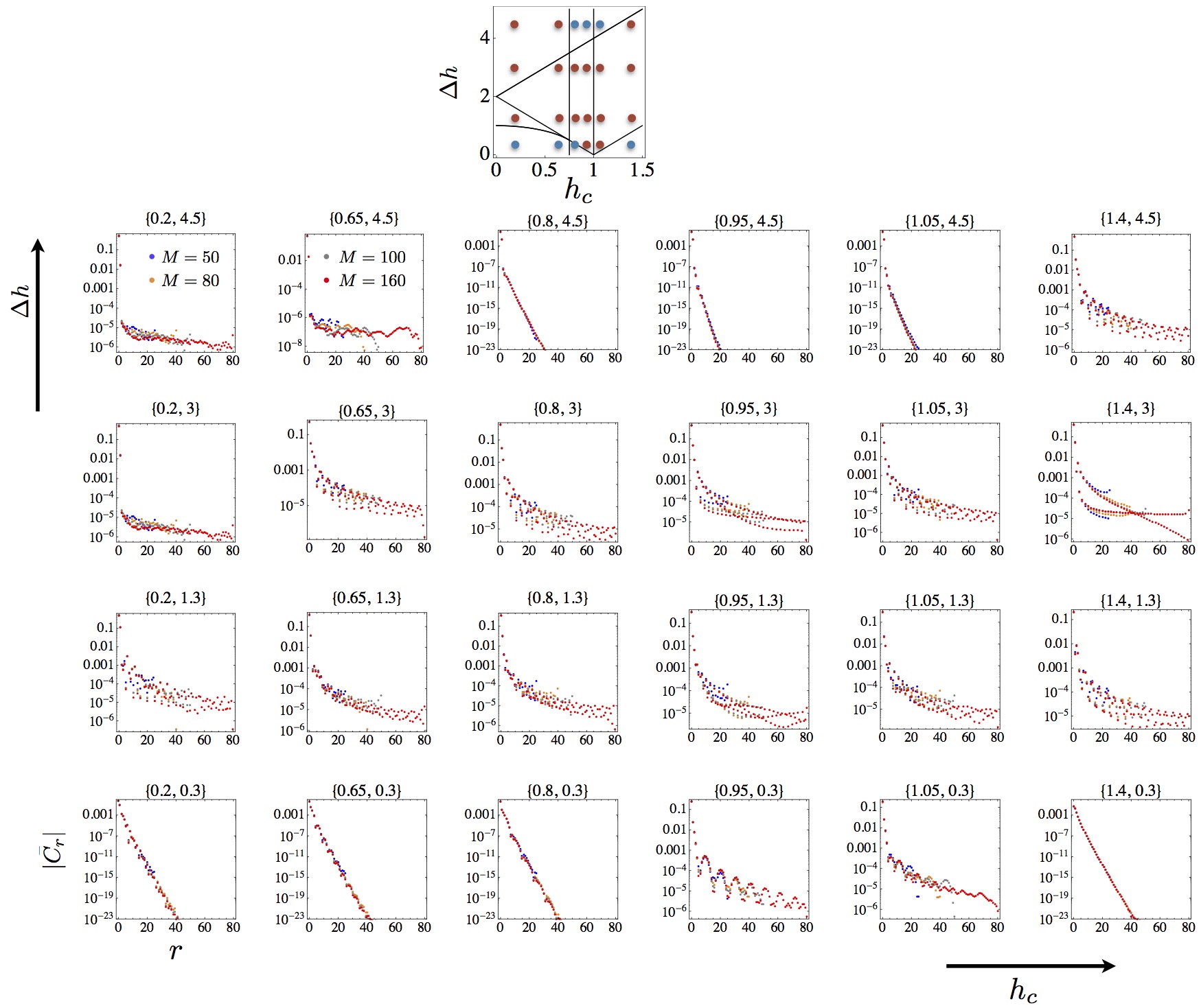
Figure 3: Upper panel: Non-equilibirum steady-state phase diagram in the $h_{c}-\Delta h$ plane. The red (blue) dots correspond to algebraic (exponential) spacial decay of the spin-spin correlation function along the $z$ direction. Lower panel: Logarithmic plots of the averaged correlation amplitudes $\bar{\left|C_{r}\right|}=\frac{2}{M}\sum_{m=M/2}^{M}\left|C_{r+m,m}\right|$ as a function of the distance between the spins, computed for different values of $h$ and $\Delta h$. Note the clear distinction between the algebraic and exponential decaying cases.

D.3 Currents

Consider a partition $\Sigma$ of the complete system under analysis with a finite range Hamiltonian and write the Hamiltonian as

$$H = H_{\Sigma}+H_{\bar{\Sigma}}+H_{\partial\Sigma}$$

where $H_{\Sigma}$ ($H_{\bar{\Sigma}}$ ) is the Hamiltonian restricted to $\Sigma$ (the complement of $\Sigma$) and $H_{\partial\Sigma}$ collects all the terms that are not separable in terms of $\Sigma$ and $\bar{\Sigma}$ degrees of freedom. A local quantity $Q$ is locally conserved if the restriction of the observable $\hat{Q}$ to the region $\Sigma$ is conserved $\left[H_{\Sigma},\hat{Q}_{\Sigma}\right]=0$. The current of the conserved quantity $Q$, leaving region $\Sigma$, is thus given by

$$\mathcal{J}_{Q,\Sigma} = -\frac{d}{dt}\left\langle Q_{\Sigma}\right\rangle=-i\left\langle\left[H,\hat{Q}_{\Sigma}\right]\right\rangle=-i\left\langle\left[H_{\partial\Sigma},\hat{Q}_{\Sigma}\right]\right\rangle.$$

Choosing $\Sigma$ to be a finite segment of an one dimensional system, the boundary Hamiltonian is made of two disjoint pieces $H_{\partial\Sigma}=H_{\partial\Sigma_{L}}+H_{\partial\Sigma_{R}}$ corresponding to the left and right boundaries. The individual left and right currents are thus given by

$$\mathcal{J}_{Q,\Sigma}^{L/R} = -i\left\langle\left[H_{\partial\Sigma_{L/R}},Q_{\Sigma}\right]\right\rangle.$$

For steady-state conditions $\mathcal{J}_{Q,\Sigma}^{R}=-\mathcal{J}_{Q,\Sigma}^{L}$.

For the energy current of the XY model, with $\Sigma$ a segment of the central region of Fig.2-(a) , we have, in terms of the Jordan-Wigner transformed fermions,

$$Q_{\Sigma} = H_{\Sigma}=-\sum_{m:\left(m,m+1\in\Sigma\right)}\frac{J}{2}\left[\left(2\gamma c_{m}^{\dagger}c_{m+1}^{\dagger}+2c_{m+1}^{\dagger}c_{m}+2c_{m}^{\dagger}c_{m+1}-2\gamma c_{m}c_{m+1}\right)\right]-h\sum_{m\in\Sigma}\left(2c_{m}^{\dagger}c_{m}-1\right)$$

$$H_{\partial\Sigma_{R}} = -\frac{J}{2}\left[\left(2\gamma c_{m}^{\dagger}c_{m+1}^{\dagger}+2c_{m+1}^{\dagger}c_{m}+2c_{m}^{\dagger}c_{m+1}-2\gamma c_{m}c_{m+1}\right)\right]\text{ with }m\in\Sigma;\,m+1\in\bar{\Sigma}$$

and

$$\mathcal{J}_{Q,\Sigma}^{R} = \frac{1}{2}C^{\dagger}\left(\begin{array}[]{cc}\boldsymbol{j}_{pp}&\boldsymbol{j}_{ph}\\ \boldsymbol{j}_{hp}&\boldsymbol{j}_{hh}\end{array}\right)C$$

with

$$\boldsymbol{j}_{pp} = -iJ^{2}\left(1-\gamma^{2}\right)\left(\left|m-1\right\rangle\left\langle m+1\right|-\left|m+1\right\rangle\left\langle m-1\right|\right)-2ihJ\left(\left|m-1\right\rangle\left\langle m\right|-\left|m\right\rangle\left\langle m-1\right|\right)$$

$$\boldsymbol{j}_{hh} = iJ^{2}\left(1-\gamma^{2}\right)\left(\left|\hat{m+1}\right\rangle\left\langle\hat{m-1}\right|-\left|\hat{m-1}\right\rangle\left\langle\hat{m+1}\right|\right)+2ihJ\left(\left|\hat{m}\right\rangle\left\langle\hat{m-1}\right|-\left|\hat{m-1}\right\rangle\left\langle\hat{m}\right|\right)$$

$$\boldsymbol{j}_{hp} = 2i\gamma hJ\left(\left|\hat{m}\right\rangle\left\langle m-1\right|-\left|\hat{m-1}\right\rangle\left\langle m\right|\right)$$

$$\boldsymbol{j}_{ph} = -2i\gamma hJ\left(\left|m-1\right\rangle\left\langle\hat{m}\right|-\left|m\right\rangle\left\langle\hat{m-1}\right|\right)$$

The mean value of the current operator can be computed as

$$\left\langle\mathcal{J}_{Q,\Sigma}^{R}\right\rangle_{t} = \frac{1}{2}\text{tr}\left\{\left(\begin{array}[]{cc}\boldsymbol{j}_{pp}&\boldsymbol{j}_{ph}\\ \boldsymbol{j}_{hp}&\boldsymbol{j}_{hh}\end{array}\right)\left[1-\boldsymbol{\chi}\left(t\right)\right]\right\}.$$

References

Kinoshita et al. (2006)T. Kinoshita, T. Wenger, and D. S. Weiss, Nature 440, 900
(2006).
Dubois et al. (2013)J. Dubois, T. Jullien,
F. Portier, P. Roche, A. Cavanna, Y. Jin, W. Wegscheider, P. Roulleau, and D. C. Glattli, Nature 502, 659 (2013).
Khajetoorians et al. (2013)A. A. Khajetoorians, B. Baxevanis, C. Hübner, T. Schlenk,
S. Krause, T. O. Wehling, S. Lounis, A. Lichtenstein, D. Pfannkuche, J. Wiebe, and R. Wiesendanger, Science (New York, N.Y.) 339, 55 (2013).