Out of equilibrium electrons and the Hall conductance of a Floquet topological insulator

Abstract

Graphene irradiated by a circularly polarized laser has been predicted to be a Floquet topological insulator showing a laser-induced quantum Hall effect. A circularly polarized laser also drives the system out of equilibrium resulting in non-thermal electron distribution functions that strongly affect transport properties. Results are presented for the Hall conductance for two different cases. One is for a closed system such as a cold-atomic gas where transverse drift due to non-zero Berry curvature can be measured in time of flight measurements. For this case the effect of a circularly polarized laser that has been switched on suddenly is studied. The second is for an open system coupled to an external reservoir of phonons. While for the former, the Hall conductance is far from the quantized limit, for the latter, coupling to a sufficiently low temperature reservoir of phonons is found to produce effective cooling, and thus an approach to the quantum limit, provided the frequency of the laser is large as compared to the band-width. For laser frequencies comparable to the band-width, strong deviations from the quantum limit of conductance is found even for a very low temperature reservoir, with the precise value of the Hall conductance determined by a competition between reservoir induced cooling and the excitation of photo-carriers by the laser. For the closed system, the electron distribution function is determined by the overlap between the initial wavefunction and the Floquet states which can result in a Hall conductance which is opposite in sign to that of the open system.

I Introduction

A corner stone in condensed matter has been the discovery of the quantum Hall effect Klitzing et al. (1980); Das Sarma and Pinczuk (1997) where electrons confined to two-dimensions ($2D$) and subjected to an external magnetic field exhibit transport properties that are remarkable in their insensitivity to material parameters. In particular for the case of the integer quantum Hall effect, the Hall conductance ($\sigma_{xy}$) is quantized in integer multiples of the universal conductance $e^{2}/h$ (i.e., $\sigma_{xy}=Ce^{2}/h$) with the integer $C$ being a geometric or topological property of the band-structure, known as the Chern number. Thouless et al. (1982); Bellissard et al. (1994); Avron et al. (1994) Not surprisingly, the discovery of this effect has lead to tremendous interest in exploring similar topologically protected transport in other systems. An important contribution in this direction was the theoretical proposal of the quantum Hall effect in the absence of a magnetic field, but in the presence of a staggered magnetic flux which still breaks time-reversal symmetry. Haldane (1988) Soon after, topologically protected transport in 2D and 3D in time-reversal preserving systems was discovered. Hasan and Kane (2010); Qi and Zhang (2011); Kane and Mele (2005); Bernevig et al. (2006) There is also now a growing interest in generalizing these concepts to strongly interacting systems. Senthil (pear)

Another intriguing class of systems are those that show topological behavior only dynamically, an example of this are the Floquet topological insulators (TIs) where a time-periodic perturbation modifies the electron hopping matrix elements in such a way as to mimic a magnetic flux. Oka and Aoki (2009); Inoue and Tanaka (2010); Kitagawa et al. (2010); Lindner et al. (2011) Since time-dependent Hamiltonians do not conserve energy, the concept of energy-levels do not exist. For the particular case of time-periodic Hamiltonians, a quasi-energy spectrum may still be constructed from the eigenvalues of the time-evolution operator over one period. Shirley (1965); Sambe (1973) In this language, Floquet TIs have bulk quasi-energy bands with non-zero Berry-curvature and Chern number, and support edge-states in confined geometries.  Oka and Aoki (2009); Inoue and Tanaka (2010); Kitagawa et al. (2010); Lindner et al. (2011); Kitagawa et al. (2011); Lindner et al. (2013); Gómez-León and Platero (2013); Katan and Podolsky (2013); Perez-Piskunow et al. (2014); Lababidi et al. (2014); Kundu et al. (2014); Quelle and Morais Smith (2014)

However there are many open questions in the study of Floquet TIs that are unique to the fact that these systems are out of equilibrium. Firstly, much of the discussion in the literature assumes that these quasi-energy levels play the same role as the true energy levels of a static Hamiltonian, which leads to theoretical predictions of quantum Hall-like quantized transport, Oka and Aoki (2009); Kitagawa et al. (2011) with strong experimental signatures of robust chiral edge transport in optical waveguides. Rechstman et al. (2013) However in a nonequilibrium system the electron distribution function, which enters in all measurable quantities, is not known apriori and depends sensitively on relaxation mechanisms, Gu et al. (2011); Kundu and Seradjeh (2013); Torres et al. (2014); Dehghani et al. (2014); Shirai et al. (2015); Iadecola and Chamon (shed) and at least on shorter time-scales, on how the external periodic drive has been switched on. Lazarides et al. (2014); Sentef et al. (shed); Goldman and Dalibard (2014); Dehghani et al. (2014); D’Alessio and Rigol (shed); Bukov and Polkovnikov (2014) Moreover, unlike static Hamiltonians, there may not even be a one to one correspondence between the Chern number of the bulk quasi-bands and the number of edge-states in the quasi-spectrum, Lababidi et al. (2014) and hence some new topological invariants may be necessary for time-periodic systems. Rudner et al. (2013); Carpentier et al. (2015) Often dissipative coupling to suitably chosen reservoirs can strongly modify topological properties Diehl et al. (2011); Budich et al. (shed) thus requiring new measures for topological order in open and dissipative systems. Uhlmann (1986); Rivas et al. (2013); Viyuela et al. (2014)

Understanding these issues is particularly important due to several experimental realizations of Floquet systems such as in optical waveguides, Rechstman et al. (2013) cold atoms in periodically modulated optical lattices, Jotzu et al. (shed) 2D Dirac fermions on the surface of a 3D TI irradiated by a circularly polarized laser, Wang et al. (2013); Onishi et al. (shed) and chiral transport in graphene irradiated by THz radiation. Karch et al. (2010, 2011)

In this paper we study graphene irradiated by a circularly polarized laser, taking into account the full time-evolution of the system, and also accounting for coupling to an external reservoir of phonons. A similar study was carried out for 2D Dirac fermions Dehghani et al. (2014) where it was shown that in the absence of coupling to an external reservoir, i.e., when the system was an ideal closed quantum system, the electron distribution function retained memory of the state before the laser was switched on, and also depended on the laser switch-on protocol. It was also shown that coupling to phonons makes the system lose memory of these initial conditions, yet the electron distribution function was still far out of equilibrium even when the phonons were an ideal reservoir. The effect of the electron distribution function on the photoemission spectra was discussed.

In this paper our goal is to study the effect of the electron distribution function on the dc Hall conductance both for an ideal closed quantum system, and for an open system. A computation of the Hall conductance requires going beyond the continuum model of Dirac fermions because the Berry curvature for a Floquet system becomes mathematically ill-defined in the continuum, in the vicinity of $k$-points where laser induced inter-band transitions are allowed. On a lattice on the other hand, even in the presence of resonances, the Berry-curvature remains well defined. Thus in this paper we generalize the treatment of Ref. Dehghani et al., 2014 to graphene with the aim of exploring the dc Hall conductance.

Usually Hall conductance is measured in solid-state systems using four terminals or leads, two for driving the current, and two transverse leads across which the voltage is measured. Datta (1997) However in cold-atomic gases one may study the Hall conductance even without leads, by applying a small potential gradient, and studying the transverse drift of the particles in time of flight measurements. Jotzu et al. (shed) Thus, our results for the closed system is applicable for such a set-up. Our results for the open system is more relevant to a solid-state device where the electron-phonon scattering is strong.

We now discuss some subtleties related to transport in two dimensions. In general the conductance and conductivity are related as conductance =conductivity$\times L^{D-2}$. Thus for $D=2$, both the conductance and conductivity become independent of the sample size, and a four terminal measurement of the conductance also measures the conductivity, the latter being typically evaluated within the linear-response Kubo formalism. At the same time, conductance of mesoscopic systems can also be computed within a Landauer formalism provided there is no inelastic scattering in the system. Datta (1997) For larger systems, where electron-electron or electron-phonon scattering becomes important, the Landauer formalism can no longer be applied.

The Landauer formalism can be generalized to time-periodic systems, Kohler et al. (2005) and this approach has been used to compute the two terminal Gu et al. (2011); Kundu et al. (2014) and four terminal Torres et al. (2014) conductance of graphene sheets irradiated by a laser. This formalism again assumes that there is no inelastic scattering, and that energy is conserved upto an integer times the laser frequency, with the electron occupation probabilities primarily determined by the overlap of the Floquet states with the states in the leads. Our treatment in this paper, employing the Kubo formalism is in the opposite limit where the sample size is large so that inelastic electron-phonon scattering is important. Thus our results are in a regime complementary to that addressed in Ref. Torres et al., 2014. In this limit of large system size, the mean chemical potential of the leads maintains the average filling (in our case we are always at half filling), while the voltage difference that maintains current flow is modeled as a small electric field maintained across the sample, and which is treated within the linear-response Kubo formalism.

The outline of the paper is as follows, in Section II the model is introduced, a Kubo formula for the dc Hall conductance is derived, and the “ideal” quantum limit explained. In Section III the dc Hall conductance is presented for the closed system and compared with the “ideal” case. In Section IV we generalize to the open system where the electrons are coupled to a phonon reservoir. The rate or kinetic equation accounting for inelastic electron-phonon scattering in the presence of a periodic drive is derived. The results for the Hall conductance at steady-state with different reservoir temperatures are obtained and compared with results for the closed system and with the ”ideal” case. Finally in section V we present our conclusions.

II Model

We study graphene irradiated by a circularly polarized laser, and also coupled to a bath of phonons. The Hamiltonian is,

$$H=H_{\rm el}+H_{\rm ph}+H_{c}$$ (1)

where (setting $\hbar=1$) $H_{\rm el}$ is the electronic part,

$$H_{\rm el}=-t_{h}\sum_{k}\begin{pmatrix}c_{kA}^{\dagger}&c_{kB}^{\dagger}\end{pmatrix}\begin{pmatrix}0&h_{k}^{AB}(t)\\ \left[h_{k}^{AB}(t)\right]^{*}&0\end{pmatrix}\begin{pmatrix}c_{kA}\\ c_{kB}\end{pmatrix},$$

$$h^{AB}_{k}(t)=\sum_{i=1,2,3}e^{ia(\vec{k}+\vec{A}(t))\cdot\vec{\delta}_{i}}$$ (2)

$\vec{\delta}_{i}$ are the nearest-neighbor unit-vectors on the graphene lattice, $\vec{\delta}_{1}=\left(\frac{1}{2},\frac{\sqrt{3}}{2}\right);\vec{\delta}_{2}=\left(\frac{1}{2},-\frac{\sqrt{3}}{2}\right);\vec{\delta}_{3}=\left(-1,0\right)$. The circularly polarized laser enters through minimal substitution $\vec{k}\rightarrow\vec{k}+\vec{A}(t)$, where

$$A_{x}(t)=\theta(t)A_{0}\cos\Omega t;A_{y}(t)=-\theta(t)A_{0}\sin\Omega t$$ (3)

We assume that the laser has been suddenly switched on at time $t=0$. This assumption holds equally well for lasers switched on over a time which is short as compared to the period $2\pi/\Omega$ of the laser.

The translation vectors $\vec{a}_{1},\vec{a}_{2}$ for graphene are $\vec{a}_{1}=\frac{a}{2}\left(3,\sqrt{3}\right);\vec{a}_{2}=\frac{a}{2}\left(3,-\sqrt{3}\right)$, while the reciprocal lattice vectors ($\vec{b}_{i}\cdot\vec{a}_{j}=2\pi\delta_{ij}$) are $\vec{b}_{1}=\frac{2\pi}{3a}\left(1,\sqrt{3}\right);\vec{b}_{2}=\frac{2\pi}{3a}\left(1,-\sqrt{3}\right)$. As written above, $h^{AB}_{k}$ is not invariant under translations by integer multiples of a reciprocal lattice vector, $\vec{k}\rightarrow\vec{k}+n_{i}\vec{b}_{i}$. In order to recover this symmetry it is convenient to make the transformation $c_{kB}\rightarrow c_{kB}e^{ia\vec{k}\cdot\vec{\delta}_{3}}$. Bernevig (2013) Then since, $a(\vec{\delta}_{1}-\vec{\delta}_{3})=\vec{a}_{1}$, $a(\vec{\delta}_{2}-\vec{\delta}_{3})=\vec{a}_{2}$, after this transformation, $h^{AB}_{k}$ becomes

$$h_{k}^{AB}(t)=e^{ia\vec{A}(t)\cdot\vec{\delta}_{3}}+\sum_{i=1,2}e^{i\vec{k}\cdot\vec{a}_{i}+ia\vec{A}(t)\cdot\vec{\delta}_{i}}$$ (4)

Dissipation affects the electron distribution and thus the topological signatures such as the Hall conductance. Here we consider dissipation due to coupling to 2D phonons

$$H_{\rm ph}=\sum_{q,i=x,y}\left[\omega_{qi}b_{qi}^{\dagger}b_{qi}\right]$$ (5)

where the electron-phonon coupling is

$$H_{c}=\sum_{{k}q\sigma,\sigma^{\prime}=A,B}c_{k\sigma}^{\dagger}\vec{A}_{\rm ph}(q)\cdot\vec{\sigma}_{\sigma\sigma^{\prime}}c_{{k}\sigma^{\prime}}$$ (6)

$$\vec{A}_{\rm ph}(q)=\left[\lambda_{x,q}\left(b_{x,q}^{\dagger}+b_{x,-q}\right),\lambda_{y,q}\left(b_{y,q}^{\dagger}+b_{y,-q}\right)\right]$$ (7)

As is standard practice, we have denoted the sub-lattice labels $A,B$ in terms of a pseudo-spin label $\sigma$, a notation that will be adopted throughout the paper. Above we have made the assumption that phonon induced scattering between electrons with different quasi-momenta do not occur. Thus electronic states at different quasi-momenta $k$ are independently coupled to the reservoir.

Moreover we will later assume that the phonons have a broad bandwidth so that inelastic scattering channels between electrons at all relevant quasi-energies and phonons are possible. While electron quasi-energies form an infinite ladder which may be regarded as photon absorption and emission side-bands, the matrix elements between different quasi-energy bands and phonons are suppressed very rapidly as the number of photon absorption and emission processes increase Dehghani et al. (2014). Thus for the laser amplitude and frequencies we will be working with, to have the most effective inelastic relaxation, it will be sufficient to consider a maximum phonon frequency $\omega_{q}^{\rm max}\simeq 6\Omega$. A circularly polarized laser also opens up a gap $\Delta$ at the Dirac points which in the high frequency limit of $A_{0}at_{h}/\Omega\ll 1$ is $\Delta\simeq 2A_{0}^{2}a^{2}t_{h}^{2}/\Omega$. Oka and Aoki (2009); Kitagawa et al. (2011) Thus we will assume that the lowest phonon frequency available is $\omega_{q}^{\rm min}\simeq\Delta$ to allow for efficient relaxation near the Dirac points.

II.1 Kubo formula for the Hall conductance

The Kubo formula for the Hall conductance is a linear response to a weak probe $\vec{A}_{\rm pr}$ that is applied over and above the circularly polarized laser $\vec{A}$. While the Kubo formalism has been employed before for Floquet systems Torres and Kunold (2005); Oka and Aoki (2009, 2011), yet we outline the derivation in order to highlight the main assumptions, and also in order to generalize the derivation to open systems like the one studied in this paper.

The electronic part of the Hamiltonian in the presence of an external laser $\vec{A}$ and a probe field $\vec{A}_{\rm pr}$ is,

$$H_{\rm el}^{\prime}=\sum_{ij\sigma\sigma^{\prime}}c_{i\sigma}^{\dagger}h_{ij}^{\sigma\sigma^{\prime}}c_{j\sigma^{\prime}}e^{-i\int_{j}^{i}\left(\vec{A}(t)+\vec{A}_{\rm pr}(t)\right)\cdot\vec{dl}}$$ (8)

Since $c_{j\sigma}=\frac{1}{\sqrt{N}}\sum_{k}e^{i\vec{k}\cdot\vec{j}}c_{k\sigma}$, we see that the vector potential corresponds to replacing $\vec{k}\rightarrow\vec{k}+\vec{A}+\vec{A}_{\rm pr}$. Taylor expanding with respect to the weak probe,

$$H_{\rm el}^{\prime}\simeq\sum_{jr\sigma\sigma^{\prime}}c_{j+r,\sigma}^{\dagger}h_{j+r,j}^{\sigma\sigma^{\prime}}(t)c_{j\sigma^{\prime}}\left(1-i\int_{j}^{j+r}\vec{A}_{\rm pr}(t)\cdot\vec{dl}\right)$$

$$=H_{\rm el}+\sum_{q}\vec{j}_{q}\cdot\vec{A}_{-q}^{\rm pr}$$ (9)

where $\vec{A}_{\rm pr}(\vec{j})=(1/\sqrt{N})\sum_{q}e^{i\vec{q}\cdot\vec{j}}\vec{A}_{q}^{\rm pr}$ and

$$\vec{j}_{q}=\frac{1}{\sqrt{N}}\sum_{k,\sigma\sigma^{\prime}}c_{k+q/2,\sigma}^{\dagger}c_{k-q/2,\sigma^{\prime}}\frac{\partial h_{k}^{\sigma\sigma^{\prime}}(t)}{\partial\vec{k}}$$ (10)

The current-current correlation function which quantifies how an electric field applied in the direction $\hat{i}$, affects the current flowing in the direction $\hat{j}$ is given by

$$R_{ij}(q,t,t^{\prime})=-i\theta(t,t^{\prime})\biggl{\langle}\Psi(t_{0})\biggl{|}\biggl{[}j_{qI}^{i}(t),j_{-qI}^{j}(t^{\prime})\biggr{]}\biggr{|}\Psi(t_{0})\biggr{\rangle}$$

where $|\Psi(t_{0})\rangle$ is the wavefunction at a certain reference time $t_{0}$, while the current operators are in the interaction representation

$$\vec{j}_{kI}(t)=U_{k}(t_{0},t)\vec{j}_{k}U_{k}(t,t_{0})$$ (12)

where $U_{k}(t,t^{\prime})$ is the time-evolution operator due to the electronic part of the Hamiltonian ($H_{\rm el}$), and is given by

$$U_{k}(t,t_{0})=\sum_{\alpha=u,d}e^{-i\epsilon_{k\alpha}(t-t_{0})}|\phi_{k\alpha}(t)\rangle\langle\phi_{k\alpha}(t_{0})|$$ (13)

Above $\epsilon_{k\alpha=u,d}$ are the quasi-energies while

$$|\phi_{k\alpha}(t)\rangle=\begin{pmatrix}\phi_{k\alpha}^{\uparrow}\\ \phi_{k\alpha}^{\downarrow}\end{pmatrix}$$ (14)

are the quasi-modes that are periodic in time. Thus, $U_{k\sigma\sigma^{\prime}}(t,t_{0})=\sum_{\alpha}e^{-i\epsilon_{k\alpha}(t-t_{0})}\phi_{k\alpha}^{\sigma}(t)\phi_{k\alpha}^{\sigma^{\prime}*}(t_{0})$, and in the interaction representation $c_{k\sigma}(t)=U_{k\sigma\sigma^{\prime}}(t,t_{0})c_{k\sigma^{\prime}}(t_{0}),c_{k\sigma}^{\dagger}(t)=c_{k\sigma^{\prime}}^{\dagger}(t_{0})U_{k\sigma^{\prime}\sigma}(t_{0},t)$. The quasi-energies $\epsilon_{k\alpha}$ represent an infinite ladder of states where $\epsilon_{k\alpha}$ and $\epsilon_{k\alpha}+m\Omega$, for any integer $m$, represent the same physical state corresponding to the Floquet quasi-modes $|\phi_{k\alpha}(t)\rangle$ and $e^{im\Omega t}|\phi_{k\alpha}(t)\rangle$ respectively. Confusion due to this over-counting can be easily avoided by noting that in all physical quantities and matrix elements, it is always the combination $e^{-i\epsilon_{k\alpha}t}|\phi_{k\alpha}(t)\rangle=|\psi_{k\alpha}\rangle$ that appears, where $|\psi_{k\alpha}\rangle$ are the solutions to the time-dependent Schrodinger equation. There are only two distinct solutions for $|\psi_{k\alpha}\rangle$ which we label as $\alpha=u,d$, while we adopt the convention that the corresponding quasi-energies lie within a Floquet Brillouin zone (BZ) $-\Omega/2<\epsilon_{k\alpha}<\Omega/2$.

Expanding the fermionic operators in the quasi-mode basis at $t_{0}$,

$$c_{kb^{\prime}}(t_{0})=\sum_{\alpha^{\prime}}\phi_{k\alpha^{\prime}}^{b^{\prime}}(t_{0})\gamma_{k\alpha^{\prime}}$$ (15)

where $\gamma^{\dagger}_{k\alpha},\gamma_{k\alpha}$ are the creation and annihilation operators for the quasi-modes at time $t_{0}$, the response function at $q=0$ is found to be

$$R_{ij}(q=0,t,t^{\prime})=-i\theta(t-t^{\prime})\frac{1}{N}\sum_{k,\alpha\beta\gamma\delta}$$

$$e^{-i(\epsilon_{k\alpha}-\epsilon_{k\beta})(t-t_{0})}e^{-i(\epsilon_{k\gamma}-\epsilon_{k\delta})(t^{\prime}-t_{0})}$$

$$\langle\phi_{k\beta}(t)|\biggl{[}\frac{\partial h_{k}(t)}{\partial{k}_{i}}\biggr{]}|\phi_{k\alpha}(t)\rangle\langle\phi_{k\delta}(t^{\prime})|\biggl{[}\frac{\partial h_{k}(t^{\prime})}{\partial{k}_{j}}\biggr{]}|\phi_{k\gamma}(t^{\prime})\rangle$$

$$\biggl{\langle}\Psi(t_{0})\biggl{|}\biggl{[}\gamma^{\dagger}_{k\beta}\gamma_{k\alpha},\gamma^{\dagger}_{k\delta}\gamma_{k\gamma}\biggr{]}\biggr{|}\Psi(t_{0})\biggr{\rangle}$$ (16)

Since the Floquet quasi-modes at any given time form a complete basis that obey

$$\left[h_{k}-i\partial_{t}\right]|\phi_{k\alpha}\rangle=\epsilon_{k\alpha}|\phi_{k\alpha}\rangle$$ (17)

the following relation holds,

$$\langle\phi_{k\beta}|\nabla h_{k}|\phi_{k\alpha}\rangle=i\partial_{t}\left[\langle\phi_{k\beta}|\nabla\phi_{k\alpha}\rangle\right]+\delta_{\alpha\beta}\nabla\epsilon_{k\alpha}$$

$$+\left(\epsilon_{k\alpha}-\epsilon_{k\beta}\right)\langle\phi_{k\beta}|\nabla\phi_{k\alpha}\rangle$$ (18)

$R_{ij}(t,t^{\prime})$ depends not only on the time difference $t-t^{\prime}$ but also on the mean time $(t+t^{\prime})/2$. In what follows we will make some approximations that are equivalent to averaging over the mean time.

The first approximation we make is to retain only diagonal components of the average below, since the off-diagonal terms will be accompanied by oscillations of the kind $e^{-i(\epsilon_{ku}-\epsilon_{kd})(t+t^{\prime})/2}$,

$$\biggl{\langle}\biggl{[}\gamma^{\dagger}_{k\beta}\gamma_{k\alpha},\gamma^{\dagger}_{k\delta}\gamma_{k\gamma}\biggr{]}\biggr{\rangle} =\delta_{\alpha,\delta}\delta_{\beta,\gamma}\biggl{[}\langle\gamma_{k\beta}^{\dagger}\gamma_{k\beta}\rangle$$ (19)

$$-\langle\gamma_{k\alpha}^{\dagger}\gamma_{k\alpha}\rangle\biggr{]}$$

Thus we obtain,

$$R_{ij}(q=0,t,t^{\prime})=-i\theta(t-t^{\prime})\sum_{k,\alpha,\beta}e^{-i(\epsilon_{k\alpha}-\epsilon_{k\beta})(t-t^{\prime})}$$

$$\biggl{[}\left(\epsilon_{k\alpha}-\epsilon_{k\beta}\right)\langle\phi_{k\beta}(t)|\frac{\partial}{\partial{k}_{i}}\phi_{k\alpha}(t)\rangle+i\partial_{t}\langle\phi_{k\beta}(t)|\frac{\partial}{\partial{k}_{i}}\phi_{k\alpha}(t)\rangle\biggr{]}$$

$$\biggl{[}-\left(\epsilon_{k\alpha}-\epsilon_{k\beta}\right)\langle\phi_{k\alpha}(t^{\prime})|\frac{\partial}{\partial{k}_{j}}\phi_{k\beta}(t^{\prime})\rangle$$

$$+i\partial_{t^{\prime}}\langle\phi_{k\alpha}(t^{\prime})|\frac{\partial}{\partial{k}_{j}}\phi_{k\beta}(t^{\prime})\rangle\biggr{]}\biggl{[}\langle\gamma_{k\beta}^{\dagger}\gamma_{k\beta}\rangle-\langle\gamma_{k\alpha}^{\dagger}\gamma_{k\alpha}\rangle\biggr{]}$$ (20)

Let us define

$$\langle\phi_{k\beta}(t)|\frac{\partial}{\partial{k}_{i}}\phi_{k\alpha}(t)\rangle=\sum_{m}e^{im\Omega t}C^{m}_{\beta i\alpha}$$ (21)

then,

$$R_{ij}(q=0,t,t^{\prime})=-i\theta(t-t^{\prime})\sum_{k,\alpha,\beta,m,m^{\prime}}e^{im\Omega t+im^{\prime}\Omega t^{\prime}}$$

$$e^{-i(\epsilon_{k\alpha}-\epsilon_{k\beta})(t-t^{\prime})}C^{m}_{\beta i\alpha}C^{m^{\prime}}_{\alpha j\beta}$$

$$\biggl{[}\epsilon_{k\alpha}-\epsilon_{k\beta}-m\Omega\biggr{]}\biggl{[}-\left(\epsilon_{k\alpha}-\epsilon_{k\beta}\right)-m^{\prime}\Omega\biggr{]}$$

$$\times\biggl{[}\langle\gamma_{k\beta}^{\dagger}\gamma_{k\beta}\rangle-\langle\gamma_{k\alpha}^{\dagger}\gamma_{k\alpha}\rangle\biggr{]}$$ (22)

Now we average over one the mean time $(t+t^{\prime})/2$ over one cycle of the laser. This is equivalent to keeping only $m^{\prime}=-m$ terms so that the results become time-translationally invariant,

$$R_{ij}(q=0,t,t^{\prime})=-i\theta(t-t^{\prime})(-1)\sum_{k,\alpha,\beta,m}e^{im\Omega t-im\Omega t^{\prime}}$$

$$\times e^{-i(\epsilon_{k\alpha}-\epsilon_{k\beta})(t-t^{\prime})}C^{m}_{\beta i\alpha}C^{-m}_{\alpha j\beta}$$

$$\biggl{[}\epsilon_{k\alpha}-\epsilon_{k\beta}-m\Omega\biggr{]}^{2}\biggl{[}\langle\gamma_{k\beta}^{\dagger}\gamma_{k\beta}\rangle-\langle\gamma_{k\alpha}^{\dagger}\gamma_{k\alpha}\rangle\biggr{]}$$ (23)

Denoting $\alpha=u,\beta=d$, and setting $m\rightarrow-m$ in one of the terms, we obtain,

$$R_{ij}(q=0,t,t^{\prime})=-i\theta(t-t^{\prime})(-1)\sum_{k,m}\biggl{[}\epsilon_{ku}-\epsilon_{kd}-m\Omega\biggr{]}^{2}$$

$$\times\biggl{(}e^{-i(\epsilon_{ku}-\epsilon_{kd}-m\Omega)(t-t^{\prime})}C^{m}_{diu}C^{-m}_{ujd}$$

$$-e^{-i(\epsilon_{kd}-\epsilon_{ku}+m\Omega)(t-t^{\prime})}C^{-m}_{uid}C^{m}_{dju}\biggr{)}\biggl{[}\langle\gamma_{kd}^{\dagger}\gamma_{kd}\rangle-\langle\gamma_{ku}^{\dagger}\gamma_{ku}\rangle\biggr{]}$$

Fourier transforming this expression,

$$R_{ij}(q=0,\omega)=\sum_{k,m}\biggl{[}\epsilon_{ku}-\epsilon_{kd}-m\Omega\biggr{]}^{2}$$

$$\biggl{[}\frac{C^{-m}_{uid}C^{m}_{dju}}{\omega+i\delta+\epsilon_{ku}-\epsilon_{kd}-m\Omega}-\frac{C^{m}_{diu}C^{-m}_{ujd}}{\omega+i\delta-(\epsilon_{ku}-\epsilon_{kd}-m\Omega)}\biggr{]}$$

$$\biggl{[}\langle\gamma_{kd}^{\dagger}\gamma_{kd}\rangle-\langle\gamma_{ku}^{\dagger}\gamma_{ku}\rangle\biggr{]}$$ (25)

For the Hall conductance, we need the combination,

$$R_{ij}(q=0,\omega)-R_{ji}(q=0,\omega)=\sum_{k,m}\biggl{[}\epsilon_{ku}-\epsilon_{kd}-m\Omega\biggr{]}^{2}$$

$$\times\biggl{(}C^{-m}_{uid}C^{m}_{dju}-C^{-m}_{ujd}C^{m}_{diu}\biggr{)}\frac{2\left(\omega+i\delta\right)}{\left(\omega+i\delta\right)^{2}-\left(\epsilon_{ku}-\epsilon_{kd}-m\Omega\right)^{2}}$$

$$\times\biggl{[}\langle\gamma_{kd}^{\dagger}\gamma_{kd}\rangle-\langle\gamma_{ku}^{\dagger}\gamma_{ku}\rangle\biggr{]}$$ (26)

Thus the dc Hall conductance is

$$\sigma_{ij}(\omega=0)=\frac{R_{ij}-R_{ji}}{2i\omega}\biggr{|}_{\omega=0}$$

$$=i\sum_{k,m}\biggl{(}C^{-m}_{uid}C^{m}_{dju}-C^{-m}_{ujd}C^{m}_{diu}\biggr{)}\biggl{[}\langle\gamma_{kd}^{\dagger}\gamma_{kd}\rangle-\langle\gamma_{ku}^{\dagger}\gamma_{ku}\rangle\biggr{]}$$

Denoting the laser period as $T_{\Omega}=2\pi/\Omega$,

$$i\sum_{m}\biggl{(}C^{-m}_{uid}C^{m}_{dju}-C^{-m}_{ujd}C^{m}_{diu}\biggr{)}=i\frac{1}{T^{2}_{\Omega}}\int_{0}^{T_{\Omega}}dt_{1}\int_{0}^{T_{\Omega}}dt_{2}\sum_{m}$$

$$e^{-im\Omega(t_{1}-t_{2})}\biggl{(}\langle\phi_{kd}(t_{1})|\frac{\partial}{\partial{k}_{j}}\phi_{ku}(t_{1})\rangle\langle\phi_{ku}(t_{2})|\frac{\partial}{\partial{k}_{i}}\phi_{kd}(t_{2})\rangle$$

$$-\langle\phi_{kd}(t_{1})|\frac{\partial}{\partial{k}_{i}}\phi_{ku}(t_{1})\rangle\langle\phi_{ku}(t_{2})|\frac{\partial}{\partial{k}_{j}}\phi_{kd}(t_{2})\rangle\biggr{)}$$ (28)

Using $\sum_{m}e^{im\Omega t}=\delta(t/T_{\Omega})$, we obtain,

$$i\sum_{m}\biggl{(}C^{-m}_{uid}C^{m}_{dju}-C^{-m}_{ujd}C^{m}_{diu}\biggr{)}=$$

$$i\frac{1}{T_{\Omega}}\int_{0}^{T_{\Omega}}dt\biggl{(}\langle\phi_{kd}(t)|\frac{\partial}{\partial{k}_{j}}\phi_{ku}(t)\rangle\langle\phi_{ku}(t)|\frac{\partial}{\partial{k}_{i}}\phi_{kd}(t)\rangle$$

$$-\langle\phi_{kd}(t)|\frac{\partial}{\partial{k}_{i}}\phi_{ku}(t)\rangle\langle\phi_{ku}(t)|\frac{\partial}{\partial{k}_{j}}\phi_{kd}(t)\rangle\biggr{)}$$

$$=i\frac{1}{T_{\Omega}}\int_{0}^{T_{\Omega}}dt\biggl{(}\langle\partial_{i}\phi_{kd}(t)|\partial_{j}\phi_{kd}(t)\rangle-\langle\partial_{j}\phi_{kd}(t)|\partial_{i}\phi_{kd}(t)\rangle\biggr{)}$$

$$=\frac{1}{T_{\Omega}}\int_{0}^{T_{\Omega}}dtF_{kd}(t)$$ (29)

where above we have used the orthonormality of the Floquet states at any given time. Thus the dc Hall conductance is,

$$\sigma_{xy}(\omega=0)=\frac{e^{2}}{2\pi h}\int_{BZ}d^{2}k\overline{F}_{kd}\left[\rho_{kd}-\rho_{ku}\right]$$ (30)

where $\overline{F}_{kd}$ is the time-average of the Berry curvature over one cycle,

$$\overline{F}_{kd}=\frac{1}{T_{\Omega}}\int_{0}^{T_{\Omega}}dt\,\,2{\rm Im}\biggl{[}\langle\partial_{y}\phi_{kd}(t)|\partial_{x}\phi_{kd}(t)\rangle\biggr{]}$$ (31)

and as expected, the Hall conductance depends on the occupation probabilities

$$\rho_{k\alpha=u,d}=\langle\gamma_{k\alpha}^{\dagger}\gamma_{k\alpha}\rangle$$ (32)

The “ideal” quantum limit corresponds to the case where $|\rho_{kd}-\rho_{ku}|=1$, so that the Hall conductance is

$$\sigma_{xy}^{\rm ideal}=C\frac{e^{2}}{h}$$ (33)

with

$$C=\frac{1}{2\pi}\int_{\rm BZ}d^{2}kF_{kd}$$ (34)

being the Chern number. It is important to note that while the Berry-curvature is time-dependent, it’s integral over the BZ is time-independent, and a topological invariant. However, once the population $\rho_{kd}-\rho_{ku}$ becomes dependent on momentum, the integral of the Berry-curvature weighted by the population is no longer a topological invariant, and depends on time. The averaging procedure outlined above corresponds to replacing the time-dependent Berry curvature by its average over one cycle.

In this paper we will study the time-averaged dc Hall conductance defined in Eq. (30) for two cases. One is when the occupation probabilities $\rho_{kd,u}$ are for the closed system with a quench switch-on protocol for the laser (section III), while the second is for the open system coupled to a reservoir, where the $\rho_{kd,u}$ will be determined from solving a kinetic equation (section IV). In order to compute the Berry curvature $F_{kd}$, we will employ the numerical approach of Ref. Fukui et al., 2005.

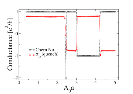
(a)

(b)

Figure 1: (Color online) Hall conductance for the ideal case ($\sigma_{xy}=Ce^{2}/h$) and for a closed system after a quench, for different strengths of the circularly polarized laser of frequency: (a). $\Omega=10t_{h}$ (b). $\Omega=5t_{h}$.

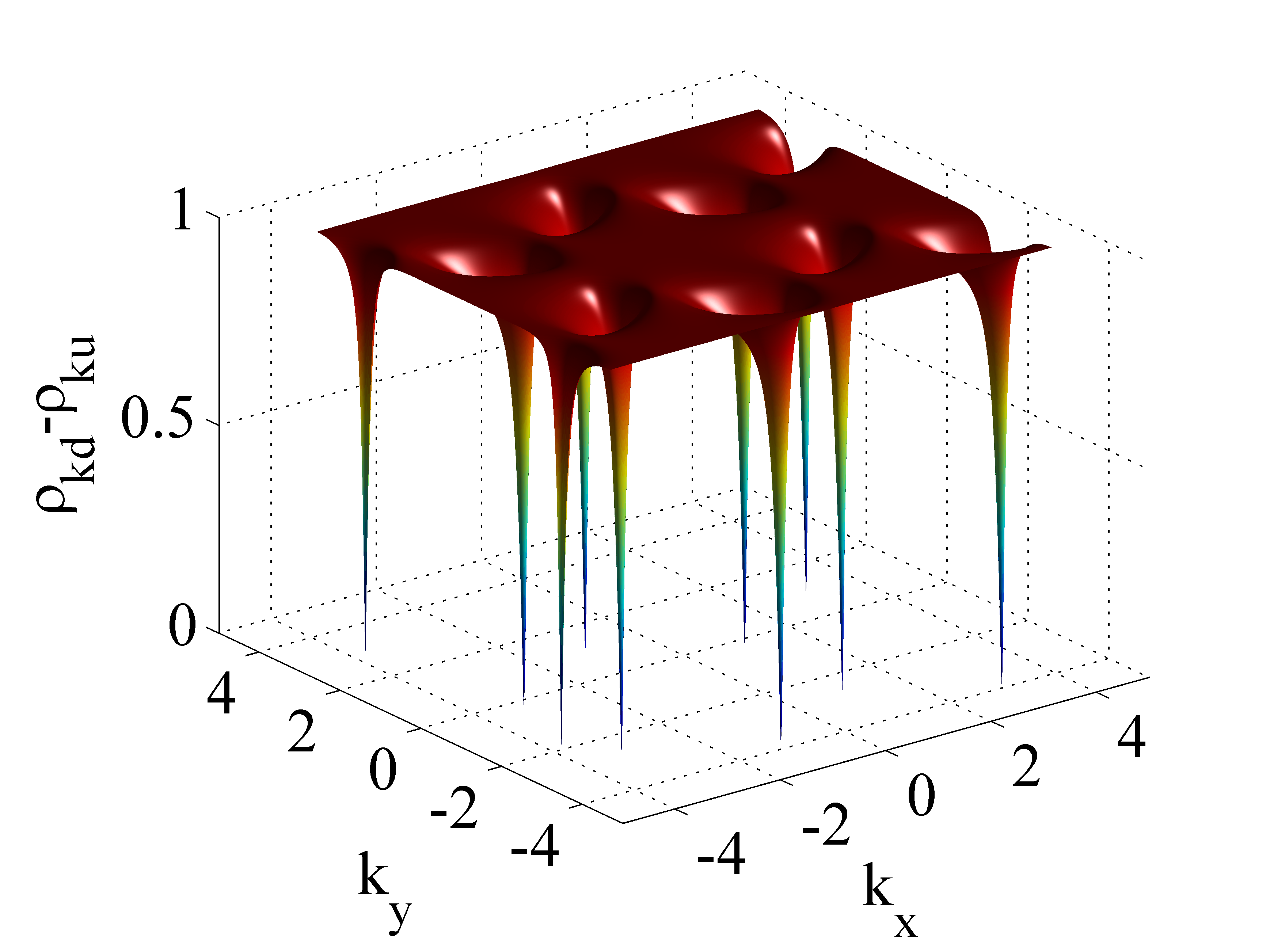
(a)

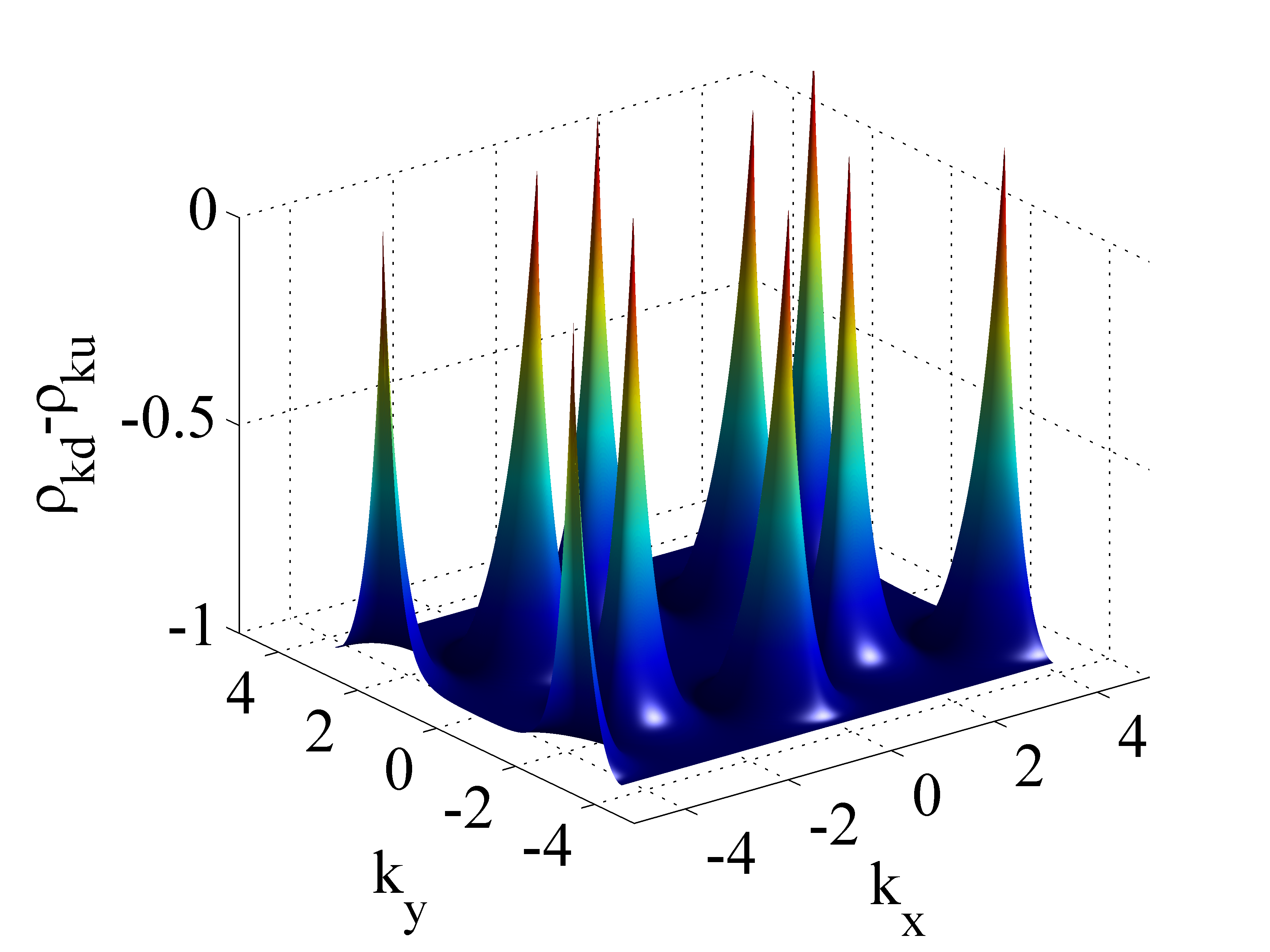
(b)

Figure 2: (Color online) Excitation density $\rho_{kd}-\rho_{ku}$ in the closed system for a quench switch-on protocol for a laser of frequency $\Omega=10t_{h}$ and amplitude: (a). $A_{0}a=1.0$ (b). $A_{0}a=5.0$.

III Hall conductance for the closed system for a quench switch-on protocol

Suppose that at $t\leq 0$, there is no external irradiation, and the electrons are in the ground-state of graphene. Thus the wavefunction right before the switching on of the laser is

$$|\Psi_{\rm in}(t=0^{-})\rangle=\prod_{{k}}|\psi_{{\rm in},k}\rangle,$$

$$|\psi_{{\rm in},k}\rangle=\frac{1}{\sqrt{2}}\begin{pmatrix}e^{i\theta_{k}}\\ 1\end{pmatrix}$$ (35)

where

$$\tan{\theta_{k}}=\frac{\sin(\vec{k}\cdot{\vec{a}}_{1})+\sin{(\vec{k}\cdot{\vec{a}}_{2})}}{1+\cos(\vec{k}\cdot{\vec{a}}_{1})+\cos{(\vec{k}\cdot{\vec{a}}_{2})}}$$ (36)

The time-evolution after switching on the laser is

$$|\Psi(t>0)\rangle=\prod_{k}U_{k}(t,0)|\psi_{\rm in,k}\rangle$$ (37)

where $U_{k}(t,t^{\prime})$ is the time-evolution operator given in Eq. (13).

In practice, in order to determine the Floquet states, it is convenient to solve the problem in Fourier space,

$$|\phi_{k\alpha}(t)\rangle=\sum_{m}e^{im\Omega t}|\tilde{\phi}_{mk\alpha}\rangle$$ (38)

where $|\tilde{\phi}_{mk\alpha}\rangle$ is a 2 component spinor which obeys,

$$\sum_{m}\left[H_{\rm el}^{nm}+m\Omega\delta_{nm}\right]|\tilde{\phi}_{mk\alpha}\rangle=\epsilon_{k\alpha}|\tilde{\phi}_{nk\alpha}\rangle,$$

$$H_{\rm el}^{nm}=\frac{1}{T_{\Omega}}\int_{0}^{T_{\Omega}}dte^{-i(n-m)\Omega t}H_{\rm el}$$

$$=\begin{pmatrix}0&h_{\sigma\sigma^{\prime}}^{nm}(k)\\ h_{\sigma^{\prime}\sigma}^{nm}(k)&0\end{pmatrix}$$ (39)

For graphene in a circularly polarized laser,

$$h^{nm}_{\sigma\sigma^{\prime}}(k)=\!\!-t_{h}i^{m-n}J_{m-n}\left(A_{0}a\right)\sum_{j=1,2,3}\!\!e^{i\vec{k}\cdot\vec{a}_{j}}e^{-i(m-n)\alpha_{j}},$$

$$h^{nm}_{\sigma^{\prime}\sigma}(k)\!\!=\!\!-t_{h}(-i)^{m-n}J_{m-n}\left(A_{0}a\right)\!\!\sum_{j=1,2,3}\!\!\!\!e^{-i\vec{k}\cdot\vec{a}_{j}}e^{-i(m-n)\alpha_{j}}$$

where $\alpha_{1}=-\alpha_{2}=\frac{\pi}{3},\alpha_{3}=\pi$ and $\vec{a}_{1}=\frac{a}{2}\left(3,\sqrt{3}\right),\vec{a}_{2}=\frac{a}{2}\left(3,-\sqrt{3}\right),\vec{a}_{3}=0$

We are interested in the time-averaged Hall conductance defined in Eq. (30). For this we need the overlap between the initial state before the quench and the Floquet quasi-modes since they control the occupation probabilities,

$$\rho_{k\alpha=u,d}^{\rm quench}=|\langle\phi_{k\alpha=u,d}(0)|\psi_{\rm in,k}\rangle|^{2}$$ (41)

Fig 1 shows the Hall conductance for the ideal case where only one Floquet band is occupied ($\rho_{kd}=1,\sigma_{xy}^{\rm ideal}=Ce^{2}/h$), and compared with the Hall conductance for the quench. Thus each point in the plot corresponds to a situation where initially the system was in the ground state of graphene, and then at time $t=0$ a laser of strength $A_{0}a$ and frequency $\Omega$ was switched on suddenly. Notice that there are a number of topological phase transitions corresponding to jumps in the Chern number as $A_{0}at_{h}/\Omega$ is varied. These topological transitions can be quite complex with the Chern number changing by $\pm 2,\pm 3$. As discussed in Ref. Kundu et al., 2014, this occurs because when linearly dispersing Dirac bands cross, the Chern number exchanges between $\pm 1$, while quadratically dispersing band-crossings cause the Chern number to exchange between $\pm 2$, and their combined effect can lead to the topological transitions observed here and in Ref. Kundu et al., 2014.

Fig. 1 shows that the Hall conductance for the closed system after a quench is smaller than that for the ideal case, this is not surprising as a quench creates a nonequilibrium population of electrons which for a closed system of non-interacting electrons, has no means to relax. The symmetry of the system dictates that the quasi-energies are located symmetrically about zero. An intriguing effect that can occur is a reversal of the sign of the Hall conductance due to a laser-like situation where the population in the “upper” quasi-band is higher. These populations are determined by the overlap of the initial wavefunction and the Floquet modes, thus as $A_{0}at_{h}/\Omega$ is varied, this overlap can be higher with one quasi-band or the other, leading to a reversal in the sign of the Hall conductance that does not necessarily follow the sign of $C$. This phenomena was also noticed in Ref. D’Alessio and Rigol, shed.

To highlight this effect, the excitation density $\rho_{kd}-\rho_{ku}$ that enters in the Hall conductance is plotted in Fig. 2 for two different cases. The upper panel of Fig. 2 is for the case where the initial wavefunction has the higher overlap with the lower (or negative energy) Floquet band so that the Hall conductance is the same sign as the ideal case, while the lower panel is for a case when the initial wavefunction has a larger overlap with the upper (positive energy) Floquet band so that the Hall conductance has the opposite sign to the ideal case. Also a very general feature of the excitation density are spikes or enhanced excitations at the Dirac points. We will show in the next section that this feature will persist even for the open system, though the spikes will broaden as the temperature of the reservoir is increased.

Another feature one finds is that the Hall conductance after a quench shows jumps that sometimes follow the topological transitions governed by jumps in $C$, but not always. For example, in the upper and lower panel of Fig. 1, one finds a topological transition at $A_{0}a\sim 2.5$ where the Chern number changes from $1\rightarrow-2\rightarrow 1$ very rapidly. The Hall conductance after the quench on the other hand is sensitive to the first transition from $1\rightarrow-2$, but not to the second from $-2\rightarrow 1$. A similar effect is seen in the lower panel in Fig. 1 where $\sigma_{xy}^{\rm quench}$ does not follow the topological transition at $A_{0}a\sim 1$.

The quench results presented here are relevant to the experimental set-up in Ref. Jotzu et al., shed where a Floquet topological system was realized in a closed cold-atomic gas, and where transport measurements were performed by tilting the system and observing the magnitude of the transverse drift in time of flight measurements. Another relevant situation is ultra-fast pump probe measurements in solids using pulse lasers, when measurements are done faster than phonon relaxation times.

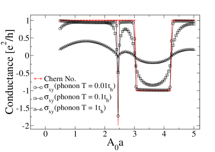
(a)

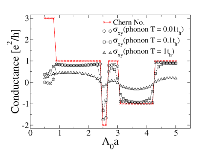
(b)

Figure 3: (Color online) Hall conductance for the ideal case ($\sigma_{xy}=Ce^{2}/h$) and at steady state with a phonon reservoir, for different strengths of the circularly polarized laser and for laser frequencies: (a). $\Omega=10t_{h}$ (b). $\Omega=5t_{h}$.

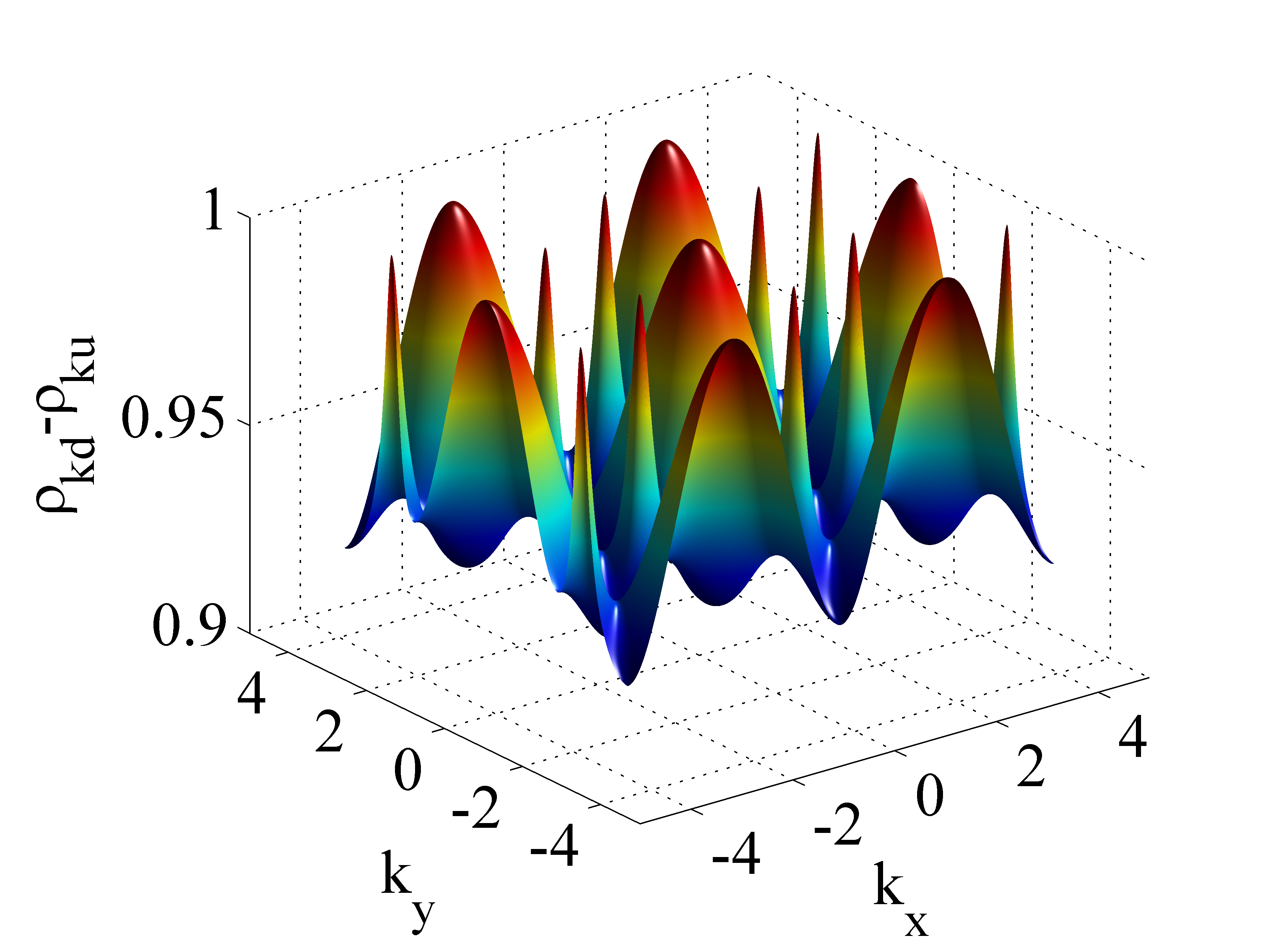
(a)

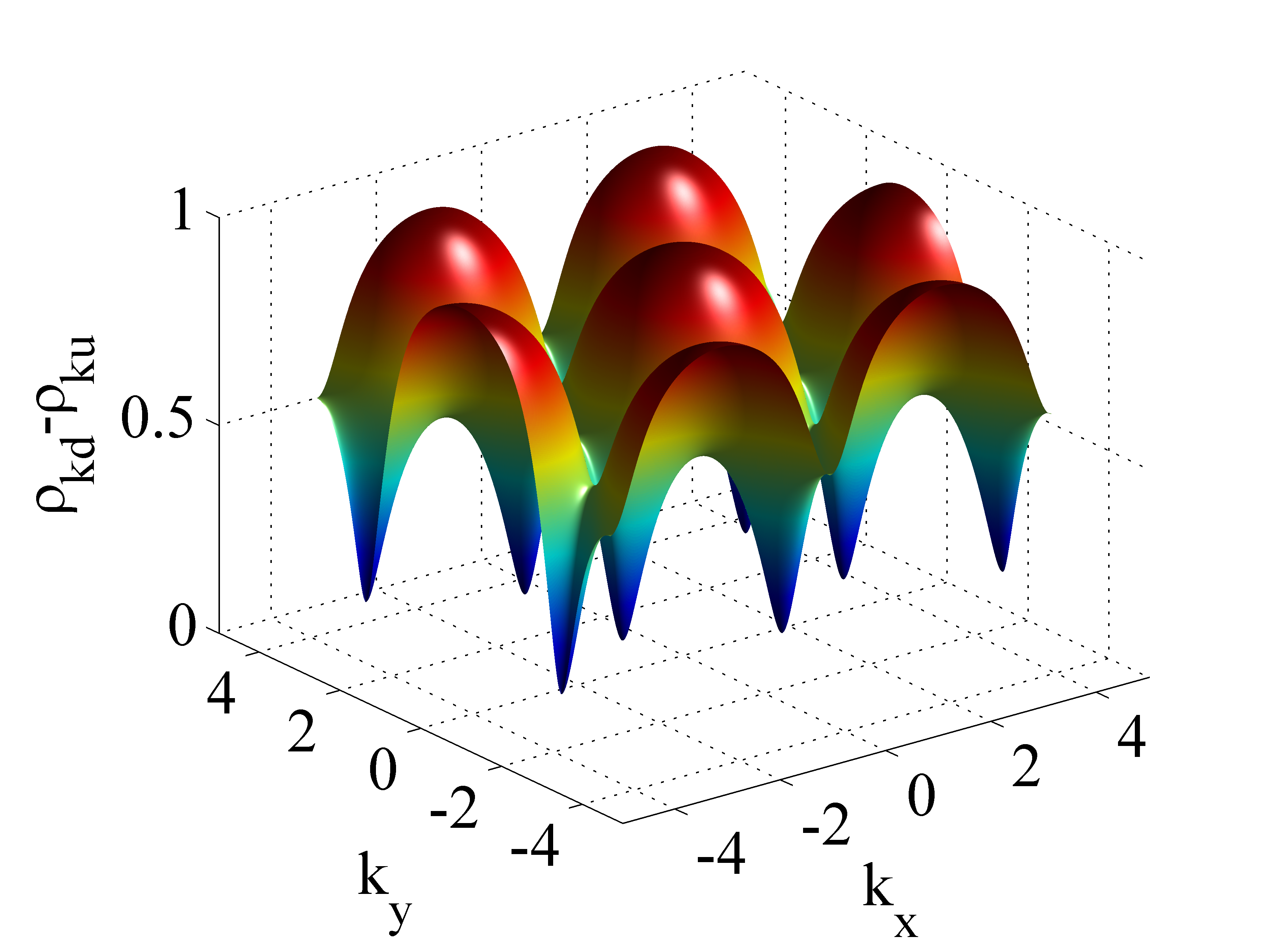
(b)

Figure 4: (Color online) Excitation density $\rho_{kd}-\rho_{ku}$ at steady state with phonons. The parameters are $A_{0}a=1.0,\Omega=10t_{h}$, with the phonons at temperature (a) $T=0.01t_{h}$, (b). $T=1.0t_{h}$.

IV Hall conductance for the open system

We now present results for the Hall conductance when the system is coupled to an ideal reservoir of phonons that is always in thermal equilibrium at a temperature $T$. Inelastic scattering between electrons and phonons will cause the electron distribution function to relax, affecting topological properties such as the Hall conductance. We employ a rate or kinetic equation approach within the Floquet formalism Kohler et al. (2005); Kohn (2001); Hone et al. (2009) to study how the electron distribution evolves from an initial state generated by a quench switch-on protocol, and present analytic results for the resulting steady-state. A similar treatment was carried out for 2D Dirac fermions irradiated by a circularly polarized laser and coupled to phonons, Dehghani et al. (2014) we generalize the approach of Ref. Dehghani et al., 2014 to graphene.

For completeness we first briefly outline the derivation of the kinetic equation. Let $W(t)$ be the density matrix obeying

$$\frac{dW(t)}{dt}=-i\left[H,W(t)\right]$$ (42)

It is convenient to be in the interaction representation, $W_{I}(t)=e^{iH_{\rm ph}t}U^{\dagger}_{\rm el}(t,0)W(t)U_{\rm el}(t,0)e^{-iH_{\rm ph}t}$, where $U_{\rm el}(t,t^{\prime})=\prod_{k}U_{k}(t,t^{\prime})$ is the time-evolution operator for the electrons under a periodic drive (see Eq. (13)). To ${\cal O}(H_{c}^{2})$, the density matrix obeys the following equation of motion

$$\frac{dW_{I}}{dt}=-i\left[H_{c,I}(t),W_{I}(t_{0})\right]$$

$$-\int_{t_{0}}^{t}dt^{\prime}\left[H_{c,I}(t),\left[H_{c,I}(t^{\prime}),W_{I}(t^{\prime})\right]\right]$$ (43)

where $H_{c,I}$ is in the interaction representation. We assume that at the initial time $t_{0}$, the electrons and phonons are uncoupled so that $W(t_{0})=W^{\rm el}_{0}(t_{0})\otimes W^{\rm ph}(t_{0})$, and that initially the electrons are in the post-quench state $|\Psi(t)\rangle$ described in Section III, while the phonons are in thermal equilibrium at temperature $T$. This is justified because phonon dynamics is much slower than electron dynamics, so that the quench state of section III can be achieved within femto-second time-scales, Wang et al. (2013) while, the phonons do not affect the system until pico-second time-scales.

Thus,

$$W^{\rm el}_{0}(t)=|\Psi(t)\rangle\langle\Psi(t)|=\prod_{k}W^{\rm el}_{k,0}$$ (44)

where

$$\!\!W^{\rm el}_{k,0}(t)=\!\!\!\sum_{\alpha,\beta=u,d}e^{-i(\epsilon_{k\alpha}-\epsilon_{k\beta})t}|\phi_{k\alpha}(t)\rangle\langle\phi_{k\beta}(t)|\rho_{k,\alpha\beta}^{\rm quench}$$ (45)

with

$$\rho_{k,\alpha\beta}^{\rm quench}=\langle\phi_{k\alpha}(0)|\psi_{{\rm in},k}\rangle\langle\psi_{{\rm in},k}|\phi_{k\beta}(0)\rangle$$ (46)

Defining the electron reduced density matrix as the one obtained from tracing over the phonons, $W^{\rm el}={\rm Tr}_{\rm ph}W$, and noting that $H_{c}$ being linear in the phonon operators, the trace vanishes, we need to solve,

$$\frac{dW^{\rm el}_{I}}{dt}=-{\rm Tr}_{\rm ph}\int_{t_{0}}^{t}dt^{\prime}\left[H_{c,I}(t),\left[H_{c,I}(t^{\prime}),W_{I}(t^{\prime})\right]\right]$$ (47)

We assume that the phonons are an ideal reservoir and stay in equilibrium. In that case $W_{I}(t)=W^{\rm el}_{I}(t)\otimes e^{-H_{\rm ph}/T}/{\rm Tr}\left[e^{-H_{\rm ph}/T}\right]$ (we set $k_{B}=1$).

The most general form of the reduced density matrix for the electrons is

$$W^{\rm el}_{I}(t)=\prod_{k}\sum_{\alpha\beta}\rho_{k,\alpha\beta}(t)|\phi_{k\alpha}(t)\rangle\langle\phi_{k\beta}(t)|$$ (48)

where in the absence of phonons, $\rho_{k,\alpha\beta}=\rho_{k,\alpha\beta}^{\rm quench}$ and are time-independent in the interaction representation. The last remaining assumption is to identify the slow and fast variables, which allows one to make the Markov approximation. Kohler et al. (2005) We assume that $\rho_{k,\alpha\beta}$ are slowly varying as compared to the characteristic time scales of the reservoir. We also make the so called modified rotating wave approximation Kohn (2001) where it is assumed that the density matrix $\rho_{k,\alpha\beta}$ varies slowly over one cycle of the laser. The last approximation is not necessary, and was not made in Ref. Dehghani et al., 2014, where it was observed that indeed the density matrix varies slowly over one cycle of the laser for sufficiently weak coupling to the reservoirs.

We only study the diagonal components of $\rho_{k,\alpha\alpha}$, which after the Markov approximation, obey the rate equation

$$\dot{\rho}_{k,\alpha\alpha}(t)=-\sum_{\beta=u,d}L^{k}_{\alpha\alpha;\beta\beta}\rho_{k,\beta\beta}(t)$$ (49)

$L^{k}_{\alpha\alpha,\beta\beta}$ are the in-scattering and out-scattering rates which due to conservation of particle number obey $\sum_{\alpha=u,d}L^{k}_{\alpha\alpha,\beta\beta}=0$.

Thus to summarize, the main approximations made in deriving Eq. (49) are Hone et al. (2009), a). the phonon bath is always in thermal equilibrium, b). the system-bath coupling is weak as compared to the laser frequency as well as the bath relaxation rates, c). the bath correlation times are short as compared to the time-scales over which the reduced density matrix for the electrons varies, d). a modified rotating wave approximation has been made where the scattering matrix elements are replaced by their average over one cycle of the laser. This is valid when the reduced density matrix varies slowly over one cycle of the laser, which is typically the case when the system-bath coupling is weak in comparison to the laser frequency. Dehghani et al. (2014) The Floquet kinetic equation fully takes into account the time-periodic structure of the Floquet states. The reduced density matrix components $\rho_{k,\alpha\alpha}$ are the occupation probabilities of these Floquet states, and it is these probabilities that are assumed to be sufficiently slowly varying in time.

While the physical initial condition corresponds to a quench switch on protocol for the laser where $\rho_{k,\alpha\alpha}(t=0)=\rho_{k,\alpha=u,d}^{\rm quench}$, the steady-state solution is independent of this initial state and corresponds to $\rho_{k,\alpha\alpha}(t=\infty)=\rho_{k\alpha}$, where

$$\rho_{ku}=\frac{|L^{k}_{uu,dd}|}{|L^{k}_{uu,dd}|+|L^{k}_{uu,uu}|};\rho_{kd}=1-\rho_{ku}$$ (50)

Expanding $\langle\phi_{k\alpha}(t)|c_{k\sigma}^{\dagger}c_{k\sigma^{\prime}}|\phi_{k\beta}(t)\rangle$ in a Fourier series such that $\langle\phi_{k\alpha}(t)|c_{k\uparrow}^{\dagger}c_{k\downarrow}|\phi_{k\beta}(t)\rangle=\sum_{n}e^{in\Omega t}C^{n}_{1k,\alpha\beta}$, and $C^{n}_{2k,\alpha\beta}=\left(C^{-n}_{1k,\beta\alpha}\right)^{*}$, we find the following in-scattering and out-scattering rates for a uniform phonon density of states $D_{\rm ph}$,

$$L^{k}_{uu,uu}=D_{\rm ph}\biggl{[}\lambda_{x}^{2}\sum_{n}\left(C^{n}_{1k,ud}C^{-n}_{1k,du}+C^{n}_{2k,ud}C^{-n}_{2k,du}+C^{n}_{1k,ud}C^{-n}_{2k,du}+C^{n}_{2k,ud}C^{-n}_{1k,du}\right)$$

$$+\lambda_{y}^{2}\sum_{n}\left(-C^{n}_{1k,ud}C^{-n}_{1k,du}-C^{n}_{2k,ud}C^{-n}_{2k,du}+C^{n}_{1k,ud}C^{-n}_{2k,du}+C^{n}_{2k,ud}C^{-n}_{1k,du}\right)\biggr{]}$$

$$\times\biggl{[}\theta(-\epsilon_{kd}+\epsilon_{ku}+n\Omega)(1+N(-\epsilon_{kd}+\epsilon_{ku}+n\Omega))+\theta(\epsilon_{kd}-\epsilon_{ku}-n\Omega)N(\epsilon_{kd}-\epsilon_{ku}-n\Omega)\biggr{]}$$ (51)

$$-L^{k}_{uu,dd}=D_{\rm ph}\biggl{[}\lambda_{x}^{2}\sum_{n}\left(C^{n}_{1k,ud}C^{-n}_{1k,du}+C^{n}_{2k,ud}C^{-n}_{2k,du}+C^{n}_{1k,ud}C^{-n}_{2k,du}+C^{n}_{2k,ud}C^{-n}_{1k,du}\right)$$

$$+\lambda_{y}^{2}\sum_{n}\left(-C^{n}_{1k,ud}C^{-n}_{1k,du}-C^{n}_{2k,ud}C^{-n}_{2k,du}+C^{n}_{1k,ud}C^{-n}_{2k,du}+C^{n}_{2k,ud}C^{-n}_{1k,du}\right)\biggr{]}$$

$$\times\biggl{[}\theta(\epsilon_{kd}-\epsilon_{ku}-n\Omega)(1+N(\epsilon_{kd}-\epsilon_{ku}-n\Omega))+\theta(-\epsilon_{kd}+\epsilon_{ku}+n\Omega)N(-\epsilon_{kd}+\epsilon_{ku}+n\Omega)\biggr{]}$$ (52)

Above $N(x)=1/(e^{x/T}-1)$ is the Bose function. In presenting our results we also consider an isotropic electron-phonon coupling $\lambda_{x}=\lambda_{y}$ so that the steady-state electron distribution function becomes independent of the electron-phonon coupling.

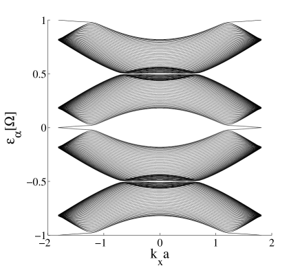
(a)

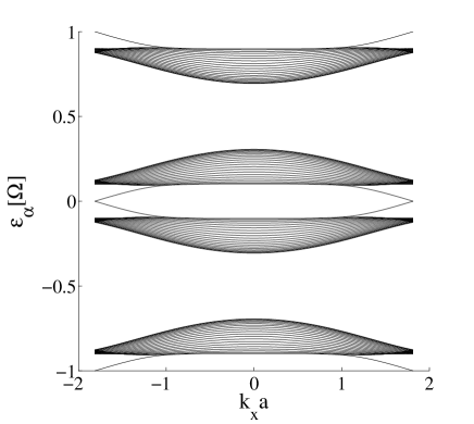
(b)

Figure 5: (Color online) Floquet spectrum over two Floquet BZs for laser frequency $\Omega=5.0t_{h}$ and for laser amplitudes and Chern numbers, (a). $A_{0}a=0.5,C=3$ (b). $A_{0}a=1.5,C=1$. Additional edge states at the Floquet zone boundaries appear for case (a).

Eqs. (51) and  (52) imply that the population of the two quasi-bands $\rho_{kd,u}$ are determined by a sum over phonon induced inelastic scattering between many quasi-energy levels (denoted by the sum over $n$). These complicated scattering processes imply a nonequilibrium (non-Gibbsian) steady-state for the electrons even when the phonons are in thermal equilibrium, unless the frequency of the laser is so high that only a single term in the sum over $n$ survives Dehghani et al. (2014); Shirai et al. (2015). In such a high-frequency limit, as we shall show, the Hall conductance approaches a thermal result, and in particular will approach $Ce^{2}/h$ as the reservoir temperature is lowered. For lower laser frequencies on the other hand, significant deviations from $Ce^{2}/h$ will be found even when the phonons are at a very low temperature.

Fig. 3 shows the steady-state Hall conductance for three different reservoir temperatures ($T=0.01t_{h},0.1t_{h},1t_{h}$), and for the same laser parameters as the ones for which the quench results were discussed. These results are plotted with those for the “ideal” case. Fig. 3 (a) is for a fairly high frequency ($\Omega=10t_{h}$) and shows that the steady-state Hall conductance approaches the ideal limit of $Ce^{2}/h$ as the temperature of the reservoir is lowered, with the topological transitions characterized by a thermal broadening. The excitation density for the same laser frequency is shown in Fig. 4, and is characterized by sharp spikes at the Dirac points at low temperatures which then show thermal broadening as the temperature of the reservoir is raised.

Fig. 3 (b) is for a lower laser frequency of $\Omega=5t_{h}$. In this case, while for large laser amplitudes ($A_{0}a>1$), the results are similar to panel (a), with the Hall conductance approaching $Ce^{2}/h$ as the temperature of the bath is lowered, marked deviations are seen for smaller laser amplitudes ($A_{0}a<1$). For this case the Hall conductance, even with low temperature phonons, saturates at a value very different from $Ce^{2}/h$, infact almost approaching zero.

Even though we have a large sample in mind, where the role played by the edges do not explicitly enter the calculation, it is still instructive to study the quasi-energy spectrum in a finite geometry (Fig. 5) to understand the difference between the case of $A_{0}a>1$ and $A_{0}a<1$, but at the same laser frequency $\Omega=5t_{h}$. One observes that $A_{0}a>1$ is also the case where the laser frequency is large as compared to the electron band-width (which is strongly influenced by $A_{0}a$), and all the edge-states reside at the center of the Floquet BZ ($\epsilon=0$), with the number of chiral edge modes equaling the Chern number $C$. In contrast for laser frequencies comparable to or smaller than the band-width, ($A_{0}a<1$), additional edge modes appear in the Floquet zone boundaries ($\epsilon=\pm\Omega/2$), and the number of chiral edge modes no longer equal the Chern number $C$, which is no longer a good or sufficient topological index. A modified topological invariant has been introduced that correctly counts the number of edges modes at the center and edges of the zone-boundary Rudner et al. (2013); Carpentier et al. (2015), however we find that the distribution function at low frequencies is so far out of equilibrium, that the Hall conductance is unrelated to this new topological invariant, and almost approaches zero. Thus highly nonequilibrium steady-states for small laser frequencies prevent one to achieve Hall conductances of ${\cal O}(e^{2}/h)$.

Fig. 6 shows how the Hall conductance depends upon the frequency of the laser for the closed as well as for the open system, where for the latter the reservoir temperature is fairly low ($T=0.01t_{h}$). As the laser frequency is increased, the Hall conductance for the open system approaches the ideal quantum limit, and the results become more and more like an equilibrium system where the Floquet bands are occupied by the Gibbs distribution. Dehghani et al. (2014); Shirai et al. (2015) The closed system of course corresponds to a nonequilibrium situation as there is no mechanism for thermalization, with the steady-state depending on the overlap between the initial state and the Floquet state, resulting in a Hall conductance that can have the opposite sign to that of the open system.

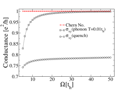
(a)

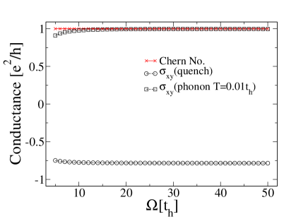
(b)

Figure 6: (Color online) Hall conductance for the closed system after a quench, for the open system at steady-state with phonons at $T=0.01t_{h}$, and for the ideal case ($Ce^{2}/h$), plotted for different laser frequencies and for the laser amplitudes: (a). $A_{0}a=1.0$ (b). $A_{0}a=5.0$.

V Conclusions

We have studied the dc Hall conductance derived from the Kubo formula, for graphene irradiated by a circularly polarized laser. Results are presented for two situations, one is for a closed system for a quench switch-on protocol for the laser, while the second is for an open system coupled to an ideal phonon reservoir. For the closed system, the electron distribution function retains memory of the initial conditions which can lead to Hall conductances (Fig. 1) that are not only smaller in magnitude than the ideal limit of $Ce^{2}/h$, but also sometimes do not follow the topological transitions in $C$ as the laser parameters are varied, and can be of the opposite sign to the ideal result. The latter occurs when the initial state has a larger overlap (Fig. 2) with the “upper” Floquet band which has a Berry curvature of the opposite sign to that of the “lower” Floquet band. The results for the closed system are most relevant for experiments in cold-atomic gases such as the one of Ref. Jotzu et al., shed.

For the open system, as long as the laser frequencies are larger than the electron bandwidth (for small laser amplitudes $A_{0}a<1$, this condition is $\Omega>6t_{h}$), the main effect of the reservoir is to cause an effective cooling that allows the Hall conductance to eventually approach $Ce^{2}/h$ as the reservoir temperature is lowered (Fig. 3, upper panel and Fig. 6), with the Hall conductance following the topological transitions with a characteristically thermal broadening.

For the open system, surprises occur for laser frequencies lower or comparable to the band-width (Fig. 3 lower panel). In this case, strong deviations of the Hall conductance from $Ce^{2}/h$ occur, with the Hall conductance almost approaching zero. This may be related to the Hall transport measured in graphene irradiated by THz laser, Karch et al. (2010, 2011) where the observed Hall effect was very small compared to the quantum limit, and was accounted for by a semi-classical Boltzman analysis.

Interestingly enough these strong deviations from the quantum limit are also accompanied by the appearance of edge-states in the BZ edges so that $C$ is no longer a good topological index. However the result we obtain cannot be accounted for by any modified topological index that takes into account these new edge modes. This is because, the electron distribution function for low laser frequencies is highly out of equilibrium even when the reservoir is ideal, with the resultant steady-state determined from solving a rate equation that accounts for laser induced photoexcitation of carriers and phonon induced inelastic scattering between many different quasi-energy levels.

These results also suggest that due to the inherent nonequilibrium nature of the problem, especially for low laser frequencies, the Hall conductance will depend upon the dominant inelastic scattering mechanism, and hence the Hall conductance in large samples where electron-phonon scattering is dominant will differ from the Hall conductance in smaller samples Torres et al. (2014) where for the latter the relaxation mechanism is determined by the location of the Fermi-levels of the leads. Gu et al. (2011); Kundu et al. (2014); Torres et al. (2014) It is of course interesting to also consider samples of intermediate size where both the leads as well as the phonons play a role in the inelastic scattering. Seetharam et al. (shed)

For the experimental feasibility of observing a large Hall response of ${\cal O}(e^{2}/h)$, one therefore needs laser frequencies larger than the electron band-width as this suppresses photoexcited carriers, and eliminates edge-states at the Floquet BZ boundaries making $C$ the relevant topological index. However, one needs to keep in mind that the maximum voltage drop across a lattice site due to the applied laser ($\sim A_{0}a\Omega$) cannot be too large in order to avoid dielectric breakdown across orbital sub-bands, at the same time the laser amplitude $A_{0}a$ should be large enough so that the dynamical gap $\Delta$ at the Dirac points is larger than the temperature of the reservoir. With current day experiments, one may realize these conditions in artificial graphene lattices such as in cold-atomic gases Jotzu et al. (shed) and photonic waveguides. Rechstman et al. (2013)

Acknowledgments: This work was supported by US Department of Energy, Office of Science, Basic Energy Sciences, under Award No. DE-SC0010821 (HD and AM).

References

- Klitzing et al. (1980) K. v. Klitzing, G. Dorda, and M. Pepper, Phys. Rev. Lett. 45, 494 (1980).
- Das Sarma and Pinczuk (1997) S. Das Sarma and A. Pinczuk, Perspectives in Quantum Hall Effects, John Wiley, New York (1997).
- Thouless et al. (1982) D. J. Thouless, M. Kohmoto, M. P. Nightingale, and M. den Nijs, Phys. Rev. Lett. 49, 405 (1982).
- Bellissard et al. (1994) J. Bellissard, A. van Elst, and H. Schulz‐ Baldes, Journal of Mathematical Physics 35 (1994).
- Avron et al. (1994) J. Avron, R. Seiler, and B. Simon, Communications in Mathematical Physics 159, 399 (1994).
- Haldane (1988) F. D. M. Haldane, Phys. Rev. Lett. 61, 2015 (1988).
- Hasan and Kane (2010) M. Z. Hasan and C. L. Kane, Rev. Mod. Phys. 82, 3045 (2010).
- Qi and Zhang (2011) X.-L. Qi and S.-C. Zhang, Rev. Mod. Phys. 83, 1057 (2011).
- Kane and Mele (2005) C. L. Kane and E. J. Mele, Phys. Rev. Lett. 95, 146802 (2005).
- Bernevig et al. (2006) B. A. Bernevig, T. L. Hughes, and S.-C. Zhang, Science 314, 1757 (2006).
- Senthil (pear) T. Senthil, arXiv:1405.4015, Annual Review of Condensed Matter Physics 6 (to appear).
- Oka and Aoki (2009) T. Oka and H. Aoki, Phys. Rev. B 79, 081406 (2009).
- Inoue and Tanaka (2010) J. Inoue and A. Tanaka, Phys. Rev. Lett. 105, 017401 (2010).
- Kitagawa et al. (2010) T. Kitagawa, E. Berg, M. Rudner, and E. Demler, Phys. Rev. B 82, 235114 (2010).
- Lindner et al. (2011) N. H. Lindner, G. Refael, and V. Galitski, Nature Physics 7, 490 (2011).
- Shirley (1965) J. H. Shirley, Phys. Rev. 138, B979 (1965).
- Sambe (1973) H. Sambe, Phys. Rev. A 7, 2203 (1973).
- Kitagawa et al. (2011) T. Kitagawa, T. Oka, A. Brataas, L. Fu, and E. Demler, Phys. Rev. B 84, 235108 (2011).
- Lindner et al. (2013) N. H. Lindner, D. L. Bergman, G. Refael, and V. Galitski, Phys. Rev. B 87, 235131 (2013).
- Gómez-León and Platero (2013) A. Gómez-León and G. Platero, Phys. Rev. Lett. 110, 200403 (2013).
- Katan and Podolsky (2013) Y. T. Katan and D. Podolsky, Phys. Rev. Lett. 110, 016802 (2013).
- Perez-Piskunow et al. (2014) P. M. Perez-Piskunow, G. Usaj, C. A. Balseiro, and L. E. F. F. Torres, Phys. Rev. B 89, 121401 (2014).
- Lababidi et al. (2014) M. Lababidi, I. I. Satija, and E. Zhao, Phys. Rev. Lett. 112, 026805 (2014).
- Kundu et al. (2014) A. Kundu, H. A. Fertig, and B. Seradjeh, Phys. Rev. Lett. 113, 236803 (2014).
- Quelle and Morais Smith (2014) A. Quelle and C. Morais Smith, Phys. Rev. B 90, 195137 (2014).
- Rechstman et al. (2013) M. Rechstman, J. Zeuner, Y. Plotnik, Y. Lumer, D. Podolsky, F. Dreisow, S. Nolte, M. Segev, and A. Szameit, Nature (London) 496, 196 (2013).
- Gu et al. (2011) Z. Gu, H. A. Fertig, D. P. Arovas, and A. Auerbach, Phys. Rev. Lett. 107, 216601 (2011).
- Kundu and Seradjeh (2013) A. Kundu and B. Seradjeh, Phys. Rev. Lett. 111, 136402 (2013).
- Torres et al. (2014) L. E. F. F. Torres, P. M. Perez-Piskunow, C. A. Balseiro, and G. Usaj, Phys. Rev. Lett. 113, 266801 (2014).
- Dehghani et al. (2014) H. Dehghani, T. Oka, and A. Mitra, Phys. Rev. B 90, 195429 (2014).
- Shirai et al. (2015) T. Shirai, T. Mori, and S. Miyashita, Phys. Rev. E 91, 030101 (2015).
- Iadecola and Chamon (shed) T. Iadecola and C. Chamon, arXiv:1412.5599 (unpublished).
- Lazarides et al. (2014) A. Lazarides, A. Das, and R. Moessner, Phys. Rev. Lett. 112, 150401 (2014).
- Sentef et al. (shed) M. A. Sentef, M. Claassen, A. F. Kemper, B. Moritz, T. Oka, J. K. Freericks, and T. P. Devereaux, arXiv:1401.5103 (unpublished).
- Goldman and Dalibard (2014) N. Goldman and J. Dalibard, Phys. Rev. X 4, 031927 (2014).
- D’Alessio and Rigol (shed) L. D’Alessio and M. Rigol, arXiv:1409.6319 (unpublished).
- Bukov and Polkovnikov (2014) M. Bukov and A. Polkovnikov, Phys. Rev. A 90, 043613 (2014).
- Rudner et al. (2013) M. S. Rudner, N. H. Lindner, E. Berg, and M. Levin, Phys. Rev. X 3, 031005 (2013).
- Carpentier et al. (2015) D. Carpentier, P. Delplace, M. Fruchart, and K. Gawedzki, Phys. Rev. Lett. 114, 106806 (2015).
- Diehl et al. (2011) S. Diehl, E. Rico, M. A. Baranov, and P. Zoller, Nature Physics 7, 971 (2011).
- Budich et al. (shed) J. C. Budich, P. Zoller, and S. Diehl, arXiv:1409.6341 (unpublished).
- Uhlmann (1986) A. Uhlmann, Rep. Math. Phys. 24, 229 (1986).
- Rivas et al. (2013) A. Rivas, O. Viyuela, and M. A. Martin-Delgado, Phys. Rev. B 88, 155141 (2013).
- Viyuela et al. (2014) O. Viyuela, A. Rivas, and M. A. Martin-Delgado, Phys. Rev. Lett. 112, 130401 (2014).
- Jotzu et al. (shed) G. Jotzu, M. Messer, R. Desbuquois, M. Lebrat, T. Uehlinger, D. Greif, and T. Esslinger, arXiv:1406.7874 (unpublished).
- Wang et al. (2013) Y. H. Wang, H. Steinberg, P. Jarillo-Herrero, and N. Gedik, Science 342, 453 (2013).
- Onishi et al. (shed) Y. Onishi, Z. Ren, M. Novak, K. Segawa, Y. Ando, and K. Tanaka, arXiv:1403.2492 (unpublished).
- Karch et al. (2010) J. Karch, P. Olbrich, M. Schmalzbauer, C. Zoth, C. Brinsteiner, M. Fehrenbacher, U. Wurstbauer, M. M. Glazov, S. A. Tarasenko, E. L. Ivchenko, D. Weiss, J. Eroms, R. Yakimova, S. Lara-Avila, S. Kubatkin, and S. D. Ganichev, Phys. Rev. Lett. 105, 227402 (2010).
- Karch et al. (2011) J. Karch, C. Drexler, P. Olbrich, M. Fehrenbacher, M. Hirmer, M. M. Glazov, S. A. Tarasenko, E. L. Ivchenko, B. Birkner, J. Eroms, D. Weiss, R. Yakimova, S. Lara-Avila, S. Kubatkin, M. Ostler, T. Seyller, and S. D. Ganichev, Phys. Rev. Lett. 107, 276601 (2011).
- Datta (1997) S. Datta, Electronic Transport in Mesoscopic Systems, Cambridge University Press (1997).
- Kohler et al. (2005) S. Kohler, J. Lehmann, and P. Hänggi, Phys. Rep. 406, 379 (2005).
- Bernevig (2013) B. A. Bernevig, Topological Insulators and Topological Superconductors, Princeton University Press (2013).
- Torres and Kunold (2005) M. Torres and A. Kunold, Phys. Rev. B 71, 115313 (2005).
- Oka and Aoki (2011) T. Oka and H. Aoki, J. Phys.:Conf. Ser. 334, 012060 (2011).
- Fukui et al. (2005) T. Fukui, Y. Hatsugai, and H. Suzuki, Journal of the Physical Society of Japan 74, 1674 (2005).
- Kohn (2001) W. Kohn, J. Stat. Phys. 103, 417 (2001).
- Hone et al. (2009) D. W. Hone, R. Ketzmerick, and W. Kohn, Phys. Rev. E 79, 051129 (2009).
- Seetharam et al. (shed) K. I. Seetharam, C.-E. Bardyn, N. H. Lindner, M. S. Rudner, and G. Refael, arXiv:1502.02664 (unpublished).