Condensates and instanton - torus knot duality. Hidden Physics at UV scale.

A. Gorsky^2,3 and A. Milekhin^1,2,3
1Institute of Theoretical and Experimental Physics, B. Cheryomushkinskaya 25, Moscow 117218, Russia

²Moscow Institute of Physics and Technology, Dolgoprudny 141700, Russia

³ Institute for Information Transmission Problems of Russian Academy of Science, B. Karetnyi 19, Moscow 127051, Russia

gorsky@itep.ru, milekhin@itep.ru

Abstract

We establish the duality between the torus knot superpolynomials or the Poincaré polynomials of the Khovanov homology and particular condensates in $\Omega$-deformed 5D supersymmetric QED compactified on a circle with 5d Chern-Simons(CS) term. It is explicitly shown that $n$-instanton contribution to the condensate of the massless flavor in the background of four-observable, exactly coincides with the superpolynomial of the $T(n,nk+1)$ torus knot where $k$ - is the level of CS term. In contrast to the previously known results, the particular torus knot corresponds not to the partition function of the gauge theory but to the particular instanton contribution and summation over the knots has to be performed in order to obtain the complete answer. The instantons are sitting almost at the top of each other and the physics of the ”fat point” where the UV degrees of freedom are slaved with point-like instantons turns out to be quite rich. Also also see knot polynomials in the quantum mechanics on the instanton moduli space. We consider the different limits of this correspondence focusing at their physical interpretation and compare the algebraic structures at the both sides of the correspondence. Using the AGT correspondence, we establish a connection between superpolynomials for unknots and q-deformed DOZZ factors.

1 Introduction

The knot invariants were introduced into the QFT framework long time ago [1] however the subject has been getting new impact during the last decade. It turns out that the knot invariants should be considered in the QFT in much more broader context. They are playing several interesting roles besides the original interpretation as the Wilson loop observables in the CS theory. New approaches to their evaluation have been developed. It was recognized in [2] that the open topological strings with Calabi-Yau target space provide an effective tool to derive the knot invariants and simultaneously knot invariants count the particular BPS states in the gauge theory. The target space for the topological string was identified with $\mathcal{O}(-1)\times\mathcal{O}(-1)\rightarrow CP_{1}$ and the knot is selected by the Lagrangian brane wrapping the Lagrangian submanifold. The boundary of the open string worldsheet is fixed at the Lagrangian submanifold in the CY internal space. The recent discussion on the topological string approach to the knot invariants can be found in [3, 4]. The simplicity of torus knots stimulated the derivation of very explicit results and representations for them[5, 2].

The progress in the knot theory brings on the scene the Khovanov-Rozansky homologies which categorize the HOMFLY polynomial. The Poincaré polynomial of the Khovanov-Rozansky homologies has been interpreted in the framework of the topological strings in [6] and it was shown that such Poincaré polynomial, called superpolynomial [7], provides the refined counting of the BPS states. The Khovanov-Rozansky homologies were also related with the space of the solutions to the topological fields theories in four and five dimensions [8, 9]. The way to evaluate the superpolynomials for some class of knots has been suggested in [10] via the refined Chern-Simons theory or equivalently the particular matrix model.

Another way the knot invariants are related with the gauge theories concerns the 3d/3d duality [11] which relates the 3d theory on the submanifold in the CY space and the 3d SUSY gauge theory. The knot complement yields the particular 3d SUSY gauge theory with some matter content. The superpolynomial is related to the partition sum of 3d theory and the parameters $(A,q,t)$ in the superpolynomial were identified with the mass and two equivariant parameters with respect to two independent rotations in $\mathbb{R}^{4}$ [12]. The relation between the partition function on the vortex and the knot polynomials has been discussed in [13]. If we introduce the defects, say 2d defect in 4d theory or 3d defect in 5d theory, any physical phenomena should be recognized equivalently from the worldvolume theories of all branes involved into configurations. This simple argument suggested long time ago [14] works well and provide some interesting crosschecks (see, for instance [15]). In particular, all knot invariants should be recognized by all participants of the configuration.

There is one more important characteristic of the knot – so-called A-polynomial and its generalization – super-A-polynomial [12] depending on the set of variables $(x,y)$ which become operators upon the quantization of the $(x,y)$ symplectic pair. The A-polynomial defines the twisted superpotential in 3d theory [12, 16]. The simplest interpretation of the $(x,y)$ variables concerns the realization of the 3d theory as the theory on the domain wall separating two 4d theories [17, 18]. They are identified with the Wilson and ’t Hooft loops variables. The nice review on the subject can be found in [19].

There was some parallel progress in mathematics concerning the homologies of the torus knots and links. In what follows we shall use quite recent results concerning superpolynomials of the torus knots and their relation with the higher $(q,t)$-Catalan numbers [20, 21, 22, 23].

Another interesting line of development motivating our consideration concerns the UV completion of the different theories and the features of the decoupling of the heavy degrees of freedom. Some phenomena can happen and we know from the textbooks that the heavy degrees of freedom decouple when the masses of the corresponding excitations get large enough with the only exception - anomaly which matters at any scale since it arises from the spectral flow. However one could wonder what happens at the non-perturbative level. The issue of the role of small size instantons in the RG was raised long time ago in QCD when the integrals over the instanton size tend to diverge. The issue of the point-like instantons is also very important in the considerations of the so-called contact terms which measure the difference between the products of the different observables in UV and IR regions (see in this context, for instance [24, 25]). Therefore some regularization is needed to handle with this region in the instanton moduli space.

There were several attempts to analyze the point-like instantons carefully imposing a kind of regularization. We can mention the freckled instantons in [26], Abelian instantons in the non-commutative gauge theories [27] and the Abelian instantons on the commutative $\mathbb{R}^{4}$ blow-upped in a few points [28]. In all these cases one could define the corresponding solutions to the equations of motion with the non-vanishing topological charges. The last example concerns the Abelian instantons in the $\Omega$-deformed abelian theory where the point-like instantons can be defined as well [29]. The different deformations provide the possibility to work with the point-like instantons in a well-defined manner. In these cases we can pose the question concerning the role of these defects in the non-perturbative RG flows.

Moreover one could ask what is the fate of the extended non=perturbative configurations which involve the heavy degrees of freedom in a non-trivial way. This issue has been examined in [30, 13, 31] where the vortex solution involving the ”heavy fields” was considered. The starting point is the superconformal theory then one adds the bi-fundamental matter. One considers the non-Abelian string in the emerging UV theory. At the next step the RG flow generated by the FI term has been analyzed and it was argued that the remnant of the UV theory is the surface operator, that is, the non-Abelian string with the infinite tension. Hence the decoupling in the non-perturbative sector for the extended object is incomplete - we obtain at the end the defect with the infinite tension which provides the boundary conditions for the fields.

The third motivation for this study has more physical origin. When investigating the superfluidity it is very useful to rotate the system since the superfluid component of the current can be extracted in this way. In the first quantization approach the density of the superfluid component is related to the correlator of the winding numbers. The $\Omega$ deformation which is essentially two independent rotations in $\mathbb{R}^{4}$ was introduced by Nekrasov to regularize the instanton moduli space. On the other hand, it allows to look at the response of the ground state of to the rotations like in superfluidity. Since the curvature of the graviphoton field is just the angular velocity we could consider the behavior of the partition function at small angular velocities $\epsilon_{1},\epsilon_{2}$. It turns out that the dependence on the angular velocities is very simple [32] and the derivative of the partition function with respect to the angular velocity yields the mean angular momentum of the system [33]. It can be seen immediately that there is non-vanishing density of the angular momentum and one could be interested in its origin. It is not a simple question what is the elementary rotator like the roton in the superfluid case in the 5d gauge theory. However no doubts it should be identified as some non-perturbative configuration related to instanton.

The starting point of our analysis is the observation made in [34] concerning the relationship between certain knots invariants and the 5d SUSY gauge theory in the $\Omega$-background with CS term at level one and matter in fundamental. It was shown that the particular correlator in $U(1)$ SQED coincides with the sum over the bottom rows of the superpolynomials of the $T_{n,n+1}$ torus knot. Contrary to the previous relations between knots and the gauge theories in this case the particular gauge theory involves the infinite sum over the torus knots.

In this paper we generalize the observation made in [34] and find the similar relation between the sums over the torus knot superpolynomials and the $U(1)$ 5d gauge theories with CS term. In more general situation the second derivative of Nekrasov partition function for 5d SQED with CS term serves as the generating function for the superpolynomial of the torus knots. It is useful to interpret the 4-observable considered in [34] in a bit different manner. We start with the superconformal 5d theory and add matter in fundamental. Then the ”Wilson loop” operator in [34] can be considered as the derivative with respect to the mass of the one-loop determinant of the matter in the fundamental at the infinite mass limit. To some extend the approach used in this paper is along the lines of development elaborated in [8, 9] where the knot homologies were interpreted in terms of the particular solutions to the equations of motion in 5D SUSY gauge theories. However from our analysis it is clear that the proper generating function for the torus knot superpolynomials implies the particular matter content in the 5D theory.

One more lesson concerns the question about the mutual back reaction of IR and UV degrees of freedom. Our answer for the torus knot superpotential involves the derivatives of the partition function in 5D theory with respect to the masses of the light and the ”regulator” flavors hence it allows the twofold interpretation. First, it can be treated as a kind of the point-like instanton renormalization of the VEV $\frac{d}{dM}\langle{\tilde{\psi}}\psi\rangle$ of the light flavor in the $\Omega$-background and is treated as the back reaction of the UV degrees of freedom on the condensate of the massless flavor. The operator has non-vanishing anomalous dimension hence to some extend the superpolynomial yields the instanton contribution to the anomalous dimensions of the composite operator. Oppositely the same correlator can be read in the opposite order and can be thought of as a kind of the backreaction of the light flavor on the defect which involves the UV degrees of freedom.

Summarizing, we shall demonstrate that the gauge theory whose $n$-instanton contribution to the particular correlator coincides with the superpolynomial of $T_{n,nk+1}$ torus knot is the $U(1)$ 5d gauge theory with one compact dimension, CS term at level $k$, 2 flavors in fundamental and one flavor in the anti-fundamental representation. One mass of the fundamental tends to zero while the second tends to infinity. The mass of the anti-fundamental is arbitrary. The remnant of the heavy flavor in the IR is the chiral ring operator.

The paper is organized as follows. In Section 2 we briefly remind the main facts concerning the 5d SQED with CS term and focus at the decoupling procedure in this theory. In Section 3 we describe the relation between the instanton contribution to the derivative of condensate of the light hyper with respect to the regulator scale and the torus knot supepolynomials. In Section 4 we attempt to interpret the result of calculation in terms of a kind of composite defect involving UV degrees of freedom. Section 5 is devoted to the consideration of the different limits for parameters involved in the picture. The interpretation of the correlator from the AGT dual Liouville theory viewpoint will be considered in Section 6. The question concerning the identification of the knot polynomials in the quantum mechanics on the instanton moduli space will be analyzed in Section 7. Our findings and the lines for the further developments are summarized in the Conclusion.

2 Supersymmetric QED with CS term

2.1 Fields, couplings, symmetries and Lagrangian with $\Omega$ deformation

Five-dimensional supersymmetric QED involves of vector field $A_{A}$, four-component Dirac spinor $\lambda$ and Higgs field $\phi$, all lying in the adjoint representation of $U(1)$. The Lagrangian reads as follows:

$$\mathcal{L}=-\frac{1}{4g^{2}}F_{AB}F^{AB}+\frac{1}{g^{2}}(\partial_{A}\phi)^{2}+\cfrac{1}{g^{2}}\bar{\lambda}\gamma^{A}\partial_{A}\lambda$$ (1)

$\gamma^{A},A=1,...,5$ are five-dimensional gamma matrices.

When looking for the superfluidity it is useful to rotate the system to feel the dissipationless component of the liquid. The same trick was used by Nekrasov [32] when introducing the $\Omega$-background which corresponds to switching on the graviphoton field whose components of curvature are identified with two independent angular velocities in $R^{4}$. The response of the partition function in the $\Omega$-deformed theory yields the gravimagnetization of the ground state or the average angular momentum of the system. To some extend it measures the ” superfluid” component of the vacuum state of the 4d gauge theory.

Let us start from the discussion of pure gauge $\mathcal{N}=2$ super Yang-Mills theory in presence of $\Omega$-background in four Euclidean dimensions. Then we will lift the theory to five-dimensions. The field content of the theory is the gauge field $A_{m}$, the complex scalar $\varphi,\bar{\varphi}$ and Weyl fermions $\Lambda^{I}_{\alpha},\bar{\Lambda}^{I}_{\dot{\alpha}}$ in the adjoint of the $U(1)$ group. Here $m=1,\dots,4$, $I=1,2$ are $SU(2)_{I}$ R-symmetry index, $\alpha,\dot{\alpha}$ are the $SU(2)_{L}\times SU(2)_{R}$ spinor indices. To introduce $\Omega$-background one can consider a nontrivial fibration of $\mathbb{R}^{4}$ over a torus $T^{2}$ [32],[35]. The six-dimensional metric is:

$$ds^{2}=2dzd\bar{z}+\left(dx^{m}+\Omega^{m}d\bar{z}+\bar{\Omega}^{m}dz\right)^{2},$$ (2)

where $(z,\bar{z})$ are the complex coordinates on the torus and the four-dimensional vector $\Omega^{m}$ is defined as:

$$\Omega^{m}=\Omega^{mn}x_{n},\qquad\Omega^{mn}=\frac{1}{2\sqrt{2}}\begin{pmatrix}0&i\epsilon_{1}&0&0\\ -i\epsilon_{1}&0&0&0\\ 0&0&0&-i\epsilon_{2}\\ 0&0&i\epsilon_{2}&0\end{pmatrix}.$$ (3)

In general if $\Omega^{mn}$ is not (anti-)self-dual the supersymmetry in the deformed theory is broken. However one can insert R-symmetry Wilson loops to restore some supersymmetry [35]:

$$A^{I}_{J}=-\frac{1}{2}\Omega_{mn}\left(\bar{\sigma}^{mn}\right)^{I}_{J}d\bar{z}-\frac{1}{2}\bar{\Omega}_{mn}\left(\bar{\sigma}^{mn}\right)^{I}_{J}dz.$$ (4)

The most compact way to write down the supersymmetry transformations and the Lagrangian for the $\Omega$-deformed theory is to introduce ’long’ scalars (do not confuse them with $\mathcal{N}=1$ superfields):

$$\Phi=\varphi+i\Omega^{m}D_{m},\qquad\bar{\Phi}=\bar{\varphi}+i\bar{\Omega}^{m}D^{m},$$ (5)

Then bosonic sector of the deformed Lagrangian reads as:

$$\begin{split}\mathcal{L}_{\Omega}=-\frac{1}{4g^{2}}F_{mn}F^{mn}+\frac{1}{g^{2}}D_{m}\Phi D^{m}\bar{\Phi}+\frac{1}{2g^{2}}\left[\Phi,\bar{\Phi}\right]^{2}=\\ -\frac{1}{4g^{2}}F_{mn}F^{mn}+\cfrac{1}{g^{2}}(\partial_{m}\phi+F_{mn}\Omega^{n})(\partial^{m}\phi-F^{mn}\Omega^{n})+\frac{1}{2g^{2}}(i\Omega^{m}\partial_{m}\bar{\phi}+i\Omega^{m}\partial_{m}\phi)^{2}\end{split}$$ (6)

We can couple this theory to fundamental hypermultiplet, which consists of two scalars $q$, $\tilde{q}$ and two Weyl fermions $\psi$ and $\tilde{\psi}$ and characterized by two masses: $m$ and $\tilde{m}$, since $\mathcal{N}=2$ hypermultiplet is build from two $\mathcal{N}=1$ hypermultiplets with opposite charges. Now the bosonic part reads as:

$$\begin{split}\mathcal{L}_{m}=-\frac{1}{4g^{2}}F_{mn}F^{mn}+\cfrac{1}{g^{2}}(\partial_{m}\phi+F_{mn}\Omega^{n})(\partial^{m}\phi-F^{mn}\Omega^{n})+\\ \cfrac{1}{2}|D_{m}q|^{2}+\cfrac{1}{2}|D_{m}\tilde{q}|^{2}+\cfrac{2}{g^{2}}(i\partial_{m}(\Omega^{m}\bar{\phi}+\Omega^{m}\phi)+g^{2}(\bar{q}q-\bar{\tilde{q}}\tilde{q}))^{2}+\\ \frac{1}{2}|(\phi-m-i\Omega^{m}D_{m})q|^{2}+\frac{1}{2}|(\phi-\tilde{m}-i\Omega^{m}D_{m})\tilde{q}|^{2}+2g^{2}|\tilde{q}q|^{2}\end{split}$$ (7)

General $\Omega$-deformation preserves only one supersymmetry[35]. It is convenient to introduce topological twist[32] and take $SU_{L}(2)$ times diagonal subgroup of $SU_{R}(2)\times SU_{I}(2)$ to be Lorentz group. Then $\Lambda^{I}_{\dot{\alpha}}$ becomes scalar $\eta$ and self-dual tensor $\chi_{IJ}$, $\Lambda^{I}_{\alpha}$ becomes vector $\psi_{I}$, and $\psi,\bar{\psi}$ becomes $\theta,\nu_{m},\omega_{mn}$. Supercharges have similar fate. The scalar supercharge $Q=Q_{\Omega}$ stays unbroken.

2.2 On Decoupling procedure

Decoupling of the heavy flavor in the 5d gauge theory is very delicate issue mainly due to the UV incompleteness of the theory. It was discussed in many studies that the naive field theory intuition fails and the purely stringy degrees of freedom like different D-branes emerge in the UV completion problem. It can be recognized in the different ways, for instance, from the viewpoint of the ADHM quantum mechanics which describes the UV physics from the viewpoint of the instanton particles. The ADHM quantum mechanics in this case involves the tiny issues at the threshold when the continuum spectrum opens. It was assumed that in this quantum mechanics the stringy degrees of freedom get manifested in the index calculations.

One more pattern of the nontrivial decoupling of the heavy degrees of freedom is provided by the 4d example of the decoupling of the heavy flavor [30]. The naive decoupling of the heavy flavor fails and one finds himself with the remnant surface operator supplemented by the operator acting in the flavor fugacity space. This operator was identified with the integrable Hamiltonian of the Calogero-Ruijsenaars type [30].

In our paper we shall meet the subtleties with the UV completion as well. W the e start with the theory with the heavy flavor and try to decouple it. During this process we get the particular 4-observable as the remnant which seems to be identified naturally with the domain wall in the $\Omega$-deformed 5d SQED. This is to some extend analogous to the 4d case however the 4-observable emerges instead of 2-observable remnant. We shall also see how the information about the UV completion can be extracted from the ADHM quantum mechanics on the instanton moduli space. The knot invariants encodes the particular set of states near threshold.

On the quantitative level we shall get the following remnant of the heavy flavor in the following way. Although we start with three matter hypermultiplets, actually we need only two of them since one has infinite mass. Now we will show that the only effect from this heavy hypermultiplet is an insertion of the operator $O=\int d^{5}x\exp(-\beta(\phi+iA_{5})$, where $\phi$ is a vector multiplet scalar and $A_{5}$ is the fifth component of the gauge field:

$$\lim_{m_{2}\rightarrow\infty}\cfrac{\exp(\beta m_{2})}{\beta}\cfrac{\partial}{\partial m_{2}}Z^{U(1)}(m_{1},m_{2},m_{3})=\langle O\rangle_{m_{1},m_{3}}^{U(1)}$$ (8)

Note that upon reduction to four dimensions $\phi+iA_{5}$ becomes complex scalar Higgs field. Suppose for a while that we are considering four-dimensional theory without $\Omega$-deformation. Then integrating out heavy hypermultiplet will produce usual Coleman-Weinberg potential

$$(\phi+m_{2})^{2}\left(\log\left(\cfrac{\phi+m_{2}}{\Lambda_{UV}}\right)-1\right)=\int_{0}^{\infty}\cfrac{dt}{t^{3}}\exp(-t(\phi+m_{2}))$$ (9)

In order to lift this expression to a five-dimensional theory[36], we have to sum over the Kaluza-Klein modes, that is, add $\cfrac{2\pi in}{R}+iA_{5}$ to $\phi+m_{2}$ and sum over $n$. This will result in

$$\operatorname{Li}_{3}\left(e^{-2\pi R(\phi+m_{2}+iA_{5})}\right)$$ (10)

Which is for large $m_{2}$ is just $\exp(-2\pi R(\phi+A_{5}+m_{2}))$ So we have reproduced eq. (8) with the operator $O=\int d^{5}x\exp\left(-\beta\left(\phi(x)+iA_{5}\right)\right)$.

When switch to the $\Omega$-deformed theory, almost all supersymmetries are broken and the chiral ring gets deformed, since conventional Higgs scalar is not equivariantly closed:

$$Q_{\Omega}\phi=\Omega^{\mu}A_{\mu}$$ (11)

Appropriate deformation of complex Higgs field $\phi$ in four-dimensions such that

$$Q_{\Omega}\Phi=0$$ (12)

was build in [35] and we claim that the $\exp(-\beta\Phi)$ with deformed $\Phi$, is exactly the operator we need even in the Omega-deformed theory. In the next section we will demonstrate this statement by a direct computation.

3 Superpolynomial of torus knots and 5d SQED

In this Section we shall explore the localization formulas for the instanton Nekrasov-like partition sums in the 5d SUSY QED. Therefore we look for the proper physical theory which would involves the knot invariants in a rational clear-cut manner. In this paper we extend the proposal formulated in [34], which relates $q,t$-Catalan numbers represented the bottom row of the superpolynomials of $T_{n,n+1}$ torus knots.

We shall evaluate the K-theoric equivariant integral over the moduli space of the instantons. It is equal to equivariant Euler characteristic of the tautological line bundle $V$ over the Hilbert scheme:

$$C_{n}(q,t)=\chi^{T}(Hilb^{n}(\mathbb{C}^{2}),\Lambda^{n}V)$$ (13)

where $q,t$ are equivariant parameters for the natural torus $T$ action on $\mathbb{C}^{2}$. $C_{n}(q,t)$ are called q,t-Catalan numbers.

First, recall some relevant mathematical results.

In [37] Haiman and Garsia introduced the following generalization of Catalan numbers:

$$C_{n}(q,t)=\sum_{\lambda:|\lambda|=n}\large{\cfrac{t^{2\sum l}q^{2\sum a}(1-t)(1-q)\prod^{0,0}(1-q^{a^{\prime}}t^{l^{\prime}})(\sum q^{a^{\prime}}t^{l^{\prime}})}{\prod(q^{a}-t^{l+1})\prod(t^{l}-q^{a+1})}}$$ (14)

where all sums and products are taken over partition $\lambda$. $l$ and $a$ denote leg and arm, whereas $l^{\prime}$ and $a^{\prime}$ denote coleg and coarm respectively. $\prod^{0,0}$ denote the omission of $(0,0)$ box. In case $q=t=1$, $C_{n}(1,1)=\cfrac{1}{n+1}\left(\begin{array}[]{c}2n\\ n\\ \end{array}\right)$

It is also useful to present the expressions for the so-called higher Catalan numbers introduced in [38]. They can be represented in terms of the Young diagrams as follows

$$C_{n}^{k}(q,t)=\sum_{\lambda:|\lambda|=n}\large{\cfrac{t^{(k+1)\sum l}q^{(k+1)\sum a}(1-t)(1-q)\prod^{0,0}(1-q^{a^{\prime}}t^{l^{\prime}})(\sum q^{a^{\prime}}t^{l^{\prime}})}{\prod(q^{a}-t^{l+1})\prod(t^{l}-q^{a+1})}}$$ (15)

In what follows we shall identify the index $k$ with the level of 5d Chern-Simons term. The shift $k\rightarrow k+1$ corresponds to the decoupling of one flavor in the 5d supersymmetric SQED.

In [22] it was shown that these numbers calculate Poincaré polynomial for a plain curve singularity corresponding to $(n+1,n)$ torus knot. Furthermore, in [20] was conjectured the following expression for a superpolynomial for $(nk+1,n)$ torus knot:

$$P(A,q,t)_{nk+1,n}=$$ (16)

$$\sum_{\lambda:|\lambda|=n}\large{\cfrac{t^{(k+1)\sum l}q^{(k+1)\sum a}(1-t)(1-q)\prod^{0,0}(1+Aq^{-a^{\prime}}t^{-l^{\prime}})\prod^{0,0}(1-q^{a^{\prime}}t^{l^{\prime}})(\sum q^{a^{\prime}}t^{l^{\prime}})}{\prod(q^{a}-t^{l+1})\prod(t^{l}-q^{a+1})}}$$

In this paper we extend the proposal formulated in [34], which relates $q,t$-Catalan numbers and certain vacuum expectation value in five-dimensional $U(1)$ gauge theory in the $\Omega$-deformation. We claim that the above superpolynomial could be obtained via five-dimensional $U(1)$ gauge theory with 2 fundamental flavors with masses $m_{f},M$, one anti-fundamental flavor with the mass $m_{a}$ and Chern-Simons term with the coupling $k$:

$$P(A,q,t)_{n,nk+1}=t^{-n/2}q^{-n/2}\cfrac{1}{1+A}\cfrac{\exp(\beta M)}{\beta^{2}}\cfrac{\partial}{\partial m_{f}}\cfrac{\partial}{\partial M}Z^{U(1)}_{n}(m_{f},m_{a},M)\biggl{|}_{m_{f}=0,\ M\rightarrow\infty}$$ (17)

where $Z^{U(1)}_{n}$ is $n$-instanton contribution to the partition function.

NB: our choice of variables is different from one adopted in [20]. We will perform the identification of variables when we discuss various limits of these formulas.

Figure 1: $\mathcal{O}(-1)\times\mathcal{O}(-1)\rightarrow\mathbb{P}^{1}$ with two blow-ups corresponding to the 5D SQED with two flavors and zero CS term

One of the dimensions is compactified on a circle with radius $\beta$. We denote the $\Omega$-background parameters by $\epsilon_{1}$ and $\epsilon_{2}$. Then

$$t=\exp(-\beta\epsilon_{1})$$ (18)

$$q=\exp(-\beta\epsilon_{2})$$ (19)

$$A=-\exp(\beta m_{a})$$ (20)

We are going to prove this relation using the refined topological vertex technique[39]. According to [40], the full partition function in the case of one fundamental flavor and one anti-fundamental flavor is given by::

$$Z^{U(1)}(m_{f},m_{a})=\large{\sum_{\lambda}(-Q)^{|\lambda|}t^{|\lambda|/2}q^{|\lambda|/2}\times}$$

$$\large{\dfrac{t^{\sum l}q^{\sum a}\prod_{i=1,j=1}^{\infty}(1-Q_{f}q^{i-1/2}t^{\lambda_{i}-j+1/2})(1-Q_{a}q^{-\lambda_{i}^{t}+j-1/2}t^{1/2-i})}{\prod(t^{l}-q^{a+1})(t^{l+1}-q^{a})}}$$ (21)

where Kähler parameters: $Q_{f}=\exp(-\beta m_{f})/\sqrt{qt},Q_{a}=\sqrt{qt}\exp(\beta m_{a})$, $Q$ defines the coupling constant via $Q=\exp(-\beta/g)$. Corresponding three-dimensional Calabi-Yau geometry is represented on the Figure 1. Perturbative part is given by:

$$Z^{U(1),pert}(m_{f},m_{a})=\prod_{i=1,j=1}^{\infty}(1-Q_{f}q^{i-1/2}t^{-j+1/2})(1-Q_{a}q^{j-1/2}t^{1/2-i})$$ (22)

Then n-instanton contribution is given by:

$$Z^{U(1)}_{n}(m_{f},m_{a})=\large{\sum_{|\lambda|=n}(-Q)^{|\lambda|}t^{|\lambda|/2}q^{|\lambda|/2}\times}$$

$$\large{\dfrac{t^{\sum l}q^{\sum a}\prod(1-\exp(-\beta m_{f})t^{l^{\prime}}q^{a^{\prime}})(1-\exp(\beta m_{a})t^{-l^{\prime}}q^{-a^{\prime}})}{\prod(t^{l}-q^{a+1})(t^{l+1}-q^{a})}}$$ (23)

Factors like

$$\prod(1-\exp(-\beta m_{f})t^{l^{\prime}}q^{a^{\prime}})$$ (24)

correspond to chiral matter contribution. $U(1)$ gauge part contributes:

$$\large{\sum_{|\lambda|=n}(-Q)^{|\lambda|}t^{|\lambda|/2}q^{|\lambda|/2}\dfrac{t^{\sum l}q^{\sum a}}{\prod(t^{l}-q^{a+1})(t^{l+1}-q^{a})}}$$ (25)

Therefore, for the superpolynomial we need:

• In order to obtain a factor $\prod^{0,0}(1-q^{a^{\prime}}t^{l^{\prime}})$ in the superpolynomial we have add a zero mass chiral multiplet and differentiate with respect to its mass.

• To obtain $\sum q^{a^{\prime}}t^{l^{\prime}}$ we take another chiral multiplet, differentiate with respect to its mass and after that we send the mass to infinity.

• Factor $\prod^{0,0}(1+Aq^{-a^{\prime}}t^{-l^{\prime}})$ comes from the anti-fundamental multiplet.

• Finally, it is well-known that the Chern-Simons action with the coupling constant $k$ contributes $t^{k\sum l}q^{k\sum a}$ - it can be easily seen in the above formulas if we remember that the Cherm-Simons term emerges as a one-loop effect from $k$ very heavy chiral multiplets. However Chern-Simons coupling affects the whole geometry. The coupling is actually given by the intersection number of two-cycles on the manifold[41, 42]. For example, the theory with coupling $k=1$ and without flavors is given by geometry $\mathcal{O}(0)\times\mathcal{O}(-2)\rightarrow\mathbb{P}^{1}$ - see Figure 2. Recall, that the $n$-instanton contribution arises from the worldsheet instanton wrapping the base $\mathbb{P}^{1}$ $n$ times. This fact suggests that the shift $1\rightarrow kn+1$ in the torus knot is actually an analogue of the Witten effect, since the instanton wraps around the other two-cycle $kn$ additional times and acquires additional charge.

Figure 2: $\mathcal{O}(0)\times\mathcal{O}(-2)\rightarrow\mathbb{P}^{1}$ geometry corresponding to 5D SQED with the Chern-Simons coupling $k=1$, but without any flavors

Now let us return to the operator $\exp(-\beta\Phi)$. Consider the term $(-1)(1-t)(1-q)\sum q^{a^{\prime}}t^{l^{\prime}}$ in the original expression for a superpolynomial. If $\lambda_{i}$ is the length of i-th row, then

$$(1-t)\sum_{i=1}(q^{\lambda_{i}}t^{i-1}-t^{i-1})=\sum_{i=1}(q^{\lambda_{i}}t^{i-1}-t^{i-1}-q^{\lambda_{i}}t^{i}+t^{i})$$ (26)

where the sum is over rows in a particular Young diagram $\lambda$. The last expression is exactly what we will obtain if we calculate the vev of $\exp(-\beta\phi)$ using Nekrasov formulas([35] eq. (4.19)) - in this approach one introduces the profile function:

$$f_{\lambda,\epsilon_{1},\epsilon_{2}}(x)=|x|+\sum_{i=1}\left(|x+\epsilon_{1}-\epsilon_{2}\lambda_{i}-\epsilon_{1}i|-|x-\epsilon_{2}\lambda_{i}-\epsilon_{1}i|-|x+\epsilon_{1}-\epsilon_{1}i|+|x-\epsilon_{1}i|\right)$$ (27)

Then contribution to the vev of $\phi^{n}$ is given by

$$\cfrac{1}{2}\int_{-\infty}^{+\infty}dx\ x^{n}f^{{}^{\prime\prime}}_{\lambda,\epsilon_{1},\epsilon_{2}}(x)$$ (28)

We see that even in the presence of Omega-deformation decoupling of the heavy flavor leads to the insertion of $\exp(-\beta\phi)$.

Now we can evaluate the whole partition function summing over the instanton contributions

$$Z^{Nek}(m,\epsilon_{1},\epsilon_{2},\beta,Q)=\sum_{n}(-Q)^{n}Z_{n}(m,\epsilon_{1},\epsilon_{2},\beta)$$ (29)

Where the whole partition function obeys some interesting equations as a function of its arguments. In the NS limit when $\epsilon_{2}=0\rightarrow t=1$ the summation of q-Catalan numbers can be performed explicitly and yields [43]:

$$P(q,Q)=\cfrac{\exp(\beta M)}{\beta^{2}}\cfrac{\partial}{\partial m_{f}}\cfrac{\partial}{\partial M}Z^{Nek}(m_{f},M,q,Q/\sqrt{q})\biggl{|}_{\ m_{f}=0,\ M\rightarrow\infty}=\frac{A_{q}(Qq^{2})}{A_{q}(Qq)}$$ (30)

where $A_{q}(s)$ is the q-Airy function:

$$A_{q}(s)=\sum_{k}\cfrac{s^{k}q^{k^{2}}}{(q;q)_{k}}$$ (31)

where $(z;q)_{k}=\prod_{l=0}^{k-1}(1-zq^{l})$ is Pochhammer symbol. This implies that the condensate obeys the following relation:

$$P(q,Q)=1-QP(q,Q)P(q,qQ)$$ (32)

Unfortunately, we do not know any field-theoretic explanation of this relation. We will return to this question when we will be discussing the stable limit $k\rightarrow\infty$.

4 The Attempt of interpretation

4.1 Point-like Abelian instantons

In this Section we shall consider the physical picture behind the duality found. It implies that we have $n$ point-like instantons sitting almost at the top of each other in the background provided by the nonlocal operator $\exp(-\beta{\Phi})$. When the $\Omega$ deformation is switched off the operator becomes local therefore the physical picture we shall try to develop should respect this property. Another suggesting argument goes as follows. Consider the limit of $\epsilon_{1},\epsilon_{2}\rightarrow 0$ when the Nekrasov partition function is reduced to the form

$$Z_{Nek}\propto\exp\left(\frac{F}{\epsilon_{1}\epsilon_{2}}\right)$$ (33)

Having in mind that $\epsilon_{1},\epsilon_{2}$ are two angular velocities the simple argument shows that there is the average angular momentum $<J>\neq 0$ in the system [33] and one could say about the gravimagnetization of the ground state. Combining these arguments we could suspect that the microscopic state we are dealing with is built from the regulator degree of freedom, is nonlocal, has instanton charge $n$ and some angular momentum. This is the qualitative description of the part of this extended object in $R^{4}\times S^{1}$.

Note that a somewhat similar situation occurs in the description of the nonperturbative effects in the ABJM model [44] where the membrane M2 instantons wrapping the (m,n) cycle in the internal space yields the corresponding contribution to the partition function at strong coupling regime. The brane interpretation of the nonpeturbative effects at weak coupling is not completely clarified in that case.

We have to combine two parts into the worldvolume of some brane. First of all let us comment what are natural configurations in D=5 which obey the required property. The first candidate is the dyonic instanton [45] or its supergravity counterpart - supertube. The dyonic instanton has the instanton charge Q , F1 charge P and D2 dipole charge/ It has the geometry of the cylinder with the distributed charge densities and its angular momentum is proportional to the product of two charges $J\propto PQ$. In the other duality frame it is presented by the D3 brane with the KK momentum [46]. In this case the defect could be represented by the M5 brane supplemented by the instanton charges.

The second candidate is the D6-D0 state which corresponds to the rotating black hole [47]. This configuration can be BPS in some region of parameters [48]. From the field theory viewpoint it represents the domain wall configuration in D=5 gauge theory which carries the additional angular momentum. In the 4d dimensional $\Omega$ -deformed gauge theory such closed domain wall does exist [43] and has the geometry of the squashed sphere $S^{3}_{b}$ where $b^{2}=\frac{\epsilon_{1}}{\epsilon_{2}}$. Therefore the candidate defect would have the worldsheet $S^{3}_{b}\times S^{1}\times M$ in this case.

In all cases we assume that the key contribution for the mechanism preventing the closed object from shrinking is the angular momentum. When the SUSY is broken in some way the additional source come from the difference between the energies providing the stabilizing pressure. It is natural to expect that the nonperturbative configuration is sensitive to the $\Omega$ background and moreover we assume that the defects like strings and domain wall have the infinite tension being proportional to the mass of the regulator. However the naive argument could fail if the very heavy object is dressed by the other instanton-like configurations which yields via dimensional transmutation the factor

$$\Lambda=M\exp\left(-c/g^{2}(M)\right)$$ (34)

and potentially could yield nonvanishing contribution.

The issue of instability which would result in expanding is more complicated. It is necessary to identify the presence or absence of the negative modes at the composite defect which is not a simple task. Is there are the odd number of negative modes at the configuration it would mean that this defect corresponds to the bounce describing the Schwinger-type process of the creation of the extended object in the graviphoton field.

4.2 From UV to IR on the defect

Recently the interesting approach for the evaluation of the superconformal indexes with the surface defects of has been suggested in [30, 13, 31]. The idea is based on the realization of the bootstrapping program via particular pattern of RG flow. The aim is to evaluate the index in some quiver-like IR theory with the defect. Instead one enlarges the theory adding the hypermultiplet in the bifundamental representation with respect to the say $SU(N)\times SU(N)$ and consider the UV theory first. Since the initial IR theory is conformal the addition hyper brings the Landau pole into the problem. The FI term is added to the Lagrangian which forces the hypermultiplet to condense and fixes the scale in the model.

At the next step one would like to decouple additional flavor in bifundamental at the scales much lower then one fixed by its condensate. The decoupling could proceed in two different ways. If the background in UV theory is trivial the decoupling goes smoothly and we return down to the initial IR theory. However one can select more elaborated way and start with the nontrivial configuration at UV scale. In [30] one selects the nonabelian vortex configuration (see [49, 45, 50] for the review). The corresponding condensate of bifundamental becomes inhomogeneous and at IR the theory becomes the same IR theory without additional hyper but with additional surface operator which now is the nonabelian string with the infinite tension.

This general picture of RG flows with the nonperturbative defects turns out to be very useful and provides new tool for the evaluation of indexes. It turns out that the index of the UV theory allows the integral representation which has the interesting pole structure. The residues of the particular poles in the index can be identified with the indexes of IR theory supplemented by the surface operators with some flux $r$. There are poles corresponding to the surface operators with the different fluxes. Moreover the index in the IR theory with the defect with flux r can be identified with the action of the particular difference operator $G_{r}$ with respect to the flavor fugacities acting on the IR index without the defects

$$I_{r}\propto G_{r}I_{0}$$ (35)

This operator was identified with the Ruijsenaars-Schneider(RS) operator known to be integrable. The trigonometric RS model is nothing but the CS theory perturbed by two Wilson loops in different directions [51](see Appendix D).

Upon deriving of the superconformal index in IR theory with defect one could be interested in the additional algebraic structure behind. It was found in [13] that the operators $G_{r}$ form a nontrivial algebra. The surface operators are realized by D2 branes with $R^{2}\times S^{1}$ worldsheet and it was demonstrated that the Wilson loop along this $S^{1}$ emerges in the CS theory on $S^{1}\times C$ where C is the curve defining the superconformal theory. The following correspondence takes place

$$G_{r}\leftrightarrow<W_{r}>$$ (36)

where the Wilson loop in the representation r is evaluated. Algebra of the operators $G_{r}$ gets mapped into the Verlinde algebra in the CS theory.

4.3 Analogy with QCD and CP(N) model

Let us comment on the related questions which can be raised in QCD and its two-dimensional ”counterpart” which shares many features of QCD [52] – $CP(N)$ sigma-model. Now we know well the origin of this correspondence – it is just the matching condition between the theory in the bulk and the worldsheet theory on the defect. The analogous problem in QCD would concern the Casher-Banks relation for the chiral condensate relating it with the spectral density of the Dirac operator $\rho(0)$.

$$\langle\bar{\psi}\psi\rangle=-\pi\rho(o)$$ (37)

The fermionic zero mode at the individual instanton is senseless in the QCD vacuum since we have strongly interacting instanton ensemble however the collective effect from the instanton ensemble yields the nonvanishing density at the origin.

Now the question parallel our study would concern the response of the quark condensate on the ”mass of the regulator M” since we are looking at the derivative of the condensate with respect to the mass of the heavy flavor M. Speaking differently we are trying to evaluate the effect of the point-like instantons at the Dirac operator spectral density. The possible arguments could look as follows. We can consider the well-known path integral representation for the quark condensate in terms of the Wilson loops (see, for instance [53])

$$\langle\bar{\psi}\psi\rangle=\sum_{paths\quad C}[DC]\langle W(C)\rangle$$ (38)

where the measure over the paths is fixed by the QCD path integral and the vev of the Wilson loop involves the averaging over all configurations of the gauge field. Therefore using this representation we could say that we are searching for the back reaction of the UV degrees of freedom at the vev of the Wilson loop.

Since from our analysis we know that the key players are the point-like instantons we could wonder how they could affect the Wilson loop. The natural conjecture sounds as follows. It is known that the Wilson loop renormalization involves the specific UV contribution from the cusps [54]. Therefore one could imagine that the point-like instantons placed at the Wilson loop induces the cusps or self-intersections of the Wilson loops and therefore yield the additional UV renormalization of the quark condensate. If this interpretation is correct it would imply that the cusp anomalous dimension which on the other hand carries the information about the anomalous dimensions of the QCD operators with the large Lorentz spin should be related with the torus knot invariants.

Another way to approach the question is to use the low-energy theorems [55]. The correlator we are looking at in the SUSY theory is now the correlator of the bilinears of the massless and the regulator fields. Due to the low-energy theorems we get

$$\int d^{4}x\langle\bar{\psi}\psi(0)\bar{\psi}_{R}\psi_{R}(x)\rangle\propto\langle\bar{\psi}\psi\rangle$$ (39)

which however knows about the ”perturbative” dilatational Ward identity and one could be interested how the point-like instantons affect this relation. We shall see later that the similar result in the SUSY case can be reformulated in the Liouville AGT side in terms of the similar low-energy theorem ”dressed” by the small instantons.

How similar problem could be posed in the non-SUSY $CP(N)$ model which can appear as the theory on the defect [56]? The analogue of the closed domain wall considered above is the kink-antikink bound state which is true excitation at the large N [57]. The analogous picture looks as follows. We have one vacuum in the non-SUSY $CP(N)$ model however there is the excited vacuum between the kink-antikink pair. Following our analysis we could conjecture that this excited vacuum is the analogue of the ”regulator vacuum” in the SUSY case separated by the kinks. Naively it involves the large scale and can just decouple but the kink and antikink can be dressed by the point-like instantons similar to the dressing of the domain walls by the instantons. As a result of dressing the finite $\Lambda$ scale emerges and the kink-antikink state remains in the spectrum.

Finally note that the chiral condensate gets generated in the QED in the external magnetic field [58]. Naively it can be traced from the summation over the lowest Landau level. The analogous question sounds as follows: is there the interplay between the fermion condensate and the high Landau levels which are a kind of regulators in this problem. Apparently more involved analysis demonstrated that the higher Landau levels matter for the condensation and there is an interplay between the IR and UV physics once again.

5 Different limits

5.1 Down to HOMFLY, Jones and Alexander

In order to compare the superpolynomial with other knot invariants, let us rewrite formulas from the previous section in a bit different notation. It is convenient to change to the following variables:

$$\cfrac{1}{\tilde{q}^{2}\tilde{t}^{2}}=q=\exp(-\beta\epsilon_{1})$$ (40)

$$\tilde{q}^{2}=t=\exp(-\beta\epsilon_{2})$$ (41)

$$\tilde{a}^{2}\tilde{t}=A=-\exp(\beta m_{a})$$ (42)

And inverse:

$$\tilde{t}=-\cfrac{1}{\sqrt{qt}}=-\exp(\beta(\epsilon_{1}+\epsilon_{2})/2)$$ (43)

$$\tilde{q}=\sqrt{t}=\exp(-\beta\epsilon_{2}/2)$$ (44)

$$\tilde{a}=\sqrt{-\sqrt{tq}A}=\exp\left(\beta\frac{2m_{a}-\epsilon_{1}-\epsilon_{2}}{4}\right)$$ (45)

• $\tilde{t}=-1$: The superpolynomial reduces to HOMFLY. On the field theory side we have $\epsilon_{1}+\epsilon_{2}=0$

• $\tilde{a}=\tilde{q}^{N}$ corresponds to the quantization condition in NS limit when there is no vev of the scalar. The mass of the antifundamental gets quantized $m_{a}=\cfrac{(2N-1)\epsilon_{2}-\epsilon_{1}}{2}$ and reduction to the bottom raw or Catalans corresponds to the semiclassical limit in NS quantization. What is more, if we take $\tilde{t}=-1$ we obtain Jones polynomial for the fundamental representation of $sl(N)$

• $\tilde{a}=1$: we obtain Poincare polynomial for Hegaard-Floer homologies and mass of the anti-fundamental multiplet reads as $m_{a}=-\cfrac{\epsilon_{1}+\epsilon_{2}}{2}$. Further specification $\tilde{t}=-1$ yields Alexander polynomial. Hence the sum over Alexanders corresponds to the condensate in the case of massless antifundamental. It has some interesting realization at the CY side summarized in the Appendix A.

5.2 Up to stable limit

Consider the limit $k\rightarrow\infty$ which yields the $T_{n,\infty}$ torus knot. At the gauge theory side it corresponds to the dominance of CS in the action.

The additional unexpected structure emerges in the stable limit [59]. It turns out that the superpolynomial allows two different ”bosonic” and ”fermionic” representations. Moreover it has the structure of the character of the very special representation in $\hat{SL(2)}$ at level 1 introduced by Feigin and Stoyanovsky.

Where $\hat{SL(2)}$ at level 1 could appear from? The possible conjecture sounds as follows. We have to recognize the knot invariants from the viewpoint of the theory on the flavor branes as well. two hypermultiplets, one in fundamental and one in antifundamental. The theory on their worldvolumes should enjoy $SL(2)$ gauge group instead of SU(2) for two fundamentals. It is the analogue of the Chiral Lagrangian realized as the worldvolume theory on the flavor branes. Similar to the QCD we have the CS term here as well and the coefficient in front of it equals to the number of colors. In our abelian case we immediately arrive at the level 1 as expected. The ”Chiral Lagrangian” in our case could have Skyrmion solutions like in QCD and we conjecture that the Feigin-Stoyanovsky representation is just representation in terms of Skyrmions.

Another question which can be asked in the stable limit is the A-polynomial. The point is that superpolynomial of uncolored $T_{n,\infty}$ torus knot gives superpolynomial of unknot colored by the n-th symmetric representation $M_{n}$:

$$P_{n,\infty}(a,q,t)=\cfrac{M_{n}(a,q,t)}{M_{1}(a,q,t)}$$ (46)

These are given by the so-called MacDonald dimensions[60]. Therefore we could investigate the dependence of the superpolynomial on the representation which is governed by the super-A-polynomia l[12] of the knot. For the unknot in the symmetric representation, in our normalization it reads as

$$\hat{A}(a,q,t,\hat{x},\hat{y})=\cfrac{ta\hat{x}-a^{-1}\hat{x}^{-1}}{\hat{x}q-\hat{x}^{-1}q^{-1}}+\sqrt{-t}\hat{y}$$ (47)

where operators $\hat{x},\hat{y}$ act as

$$\hat{y}M_{n}=M_{n+1},\ \hat{x}M_{n}=(-tq)^{n}M_{n}$$ (48)

and quantum A-polynomial annihilates superpolynomial:

$$\hat{A}M_{n}=0$$ (49)

Note that this equation actually connects two different instanton contributions $M_{n}$ and $M_{n+1}$. Recall that in the NS limit $\epsilon_{2}=0$ but for a generic $k$, we have found similar relation (32) which relates different instanton contributions too. These relations are similar in the spirit to non-perturbative Dyson-Schwinger equations introduced recently by N. Nekraso v[29]. We hope to discuss this issue elsewhere [61].

5.3 Nabla - Shift - Cut-and-join operator and the decoupling of heavy flavor

Let us make few comments concerning the role of operator providing the transformation $k\rightarrow k+1$ in our picture. It has different reincarnations and different names in the several problems. It is known as Nabla operator in the theory of the symmetric functions, as the shift operator in the rational DAHA and Calogero model and cut-in-join operator in the context of some counting problems in geometry. Since we have identified this parameter as the level of 5D CS term we could use this knowledge and see the different interpretations of this shift.

From the physical side it can be immediately recognize as the effect of the decoupling of the heavy flavor since it is know for a while [62] that one-loop effect provides this shift of the level. It provides the shift of the Calogero coupling constant in the quantum mechanics on the instanton moduli space and more formally it corresponds to the multiplication of the integrand over the instanton moduli by the determinant bundle [63]. It can be also seen at the CY side when it corresponds to the change of the geometry.

In the consider action on the $T_{n,nk+1}$ torus knots this operator was used [60] to generate a kind of the discrete Hamiltonian evolution in k with the simple boundary condition for k=0, corresponding to unknot. Having in mind that the dynamics of the Calogero coupling can be interpreted as the realization of the RG evolution with the limit cycles [64] it would be interesting to look for the cyclic solutions to this discrete Hamiltonian dynamics and possible Efimov-like states in this framework.

To illustrate these arguments let us consider the limit $m_{a}\rightarrow\infty$, that is $A\rightarrow+\infty$. From physical viewpoint, we integrate out antifundamental multiplet, so the Chern-Simons coupling should reduce by one. Indeed, the following limit is well-defined:

$$\lim_{A\rightarrow+\infty}\cfrac{1}{A^{n-1}}P(A,q,t)_{nm+1,n}=P(A=0,q,t)_{n(m-1)+1,n}$$ (50)

Actually, this relation is known in the knot theory and is quite general:

$$\lim_{A\rightarrow+\infty}\cfrac{1}{A^{n-1}}P(A,q,t)_{k,n}=constP(A=0,q,t)_{k-n,n}$$ (51)

The cut-and-join operator was identified in [60] as the $W^{3}_{0}$ generator from $W^{3}$ algebra. This fits well with the our consideration since the CS term written in superfield looks as follows

$$\delta L_{CS}=\int d^{5}xd^{4}\theta\Phi^{3}$$ (52)

It is possible to develop the matrix model of the Dijkgraaf-Vafa type for the 5D gauge theory [42] which can be considered as the generation function for the superpolynomials of the $T_{n,nK+1}$ torus knots. The matrix model evaluation of the particular observable in the general case of all nonvanishing masses looks as

$$Z_{matr}=\int[dM]O(m_{1})O(m_{2})O(m_{3})exp(t_{2}TrM^{2}+t_{3}TrM^{3})$$ (53)

with some measure probably suggested in [10] and the coefficient $t_{3}$ corresponds to the CS term. It is clear that in the matrix model framework it is coupled to the corresponding $W^{3}_{0}$ generator. The knot invariants presumably can be evaluated upon taking derivatives with respect to $m_{1},m_{2}$ and the corresponding limits. The operators O(m) are conjectured to be

$$O(m)=det(M-m)$$ (54)

which can be evidently related with the resolvents. The type of the knot presumably is selected by the corresponding term of expansion in $t_{2}$ with fixed value of $t_{3}$.

Therefore the shift operator can be thought of as one of the consequences from the generalized Konishi relation in the 5D gauge theory yielding the W-constraints in the matrix model. If one introduces more times more general Virasoro and W- constraints can be formulated for the torus knots superpolynomials (see [65] for the related discussion). Let us emphasize that the matrix model with the cubic potential is different from the matrix model developed for the evaluation of the torus knot invariants from the type B topological strings in [3, 4].

6 AGT conjecture prospective

In this section we will continue our study of the five-dimensional SQED with two fundamental flavors in the $\Omega$ deformation. We will show in a moment that the instanton partition function for 5D SQED is directly related to the perturbative partition function for 5D $SU(2)$ gauge theory. Therefore, according to the AGT conjecture[66], there should be a relation between three-point functions in Liouville theory and five-dimensional SQED. We will establish an explicit connection between 5D SQED and the three-point function in the q-deformed Liouville theory on a sphere. We argue that the three-point function is equal to the combination of four instanton partition functions. Using these results we will show that there is a relation between superpolynomials for unknot and Liouville theree-point functions.

Let us consider $D=5,\ \mathcal{N}=1\ SU(2)$ gauge theory with four flavours. It can be obtained as a theory living on a certain IIB $(p,q)$-brane web - see Figure 3. Or, equivalently, as M-theory compactification on the toric Calabi-Yau theefold, those toric diagram is given by the same figure.

Figure 3: $SU(2)$ theory with four flavours

We can obtain two copies of 5D SQED by sending Coloumb parameter to infinity $a\rightarrow+\infty(Q_{c}\rightarrow 0)$, that is, by cutting the toric diagram by horizontal line - compare the result with Figure 2. If we send $g^{2}\rightarrow\infty(Q\rightarrow 0)$ then the partition function is given only by the perturbative contribution - we cut the toric diagram by vertical line - see Figure 4

Figure 4: Perturbative $SU(2)$ theory with four flavours

Note that the $SU(2)$ theory has a rotational symmetry(fiber-base duality)[67, 68, 69] which interchanges coupling constant $Q=\exp(-\beta/g^{2})$ with Coloumb parameter $Q_{f}=\exp(-\beta a)$. It is this symmetry which relates perturbative $SU(2)$ theory with instanton $U(1)$ - one has to rotate Figure 4 by 90 degrees in order to obtain Figure 2

In the pioneer work [66] it was shown that the perturbative part of the Nekrasov partition function for the four-dimensional $SU(2)$ theory with four fundamental flavors actually coincides with the three-point function $\langle e^{2\alpha_{1}\phi}e^{2\alpha_{2}\phi}e^{2\alpha_{3}\phi}\rangle$ in the Liouville theory on a sphere, also known as a DOZZ factor [70, 71]:

$$\begin{split}C(\alpha_{1},\alpha_{2},\alpha_{3})=(\pi\mu\gamma(b^{2})b^{2-2b^{2}})^{(Q-\alpha_{1}-\alpha_{2}-\alpha_{3})/b}\times\\ \cfrac{\Upsilon^{\prime}(0)\Upsilon(2\alpha_{1})\Upsilon(2\alpha_{2})\Upsilon(2\alpha_{3})}{\Upsilon(\alpha_{1}+\alpha_{2}+\alpha_{3}-Q_{c})\Upsilon(\alpha_{1}+\alpha_{2}-\alpha_{3})\Upsilon(\alpha_{1}+\alpha_{3}-\alpha_{2})\Upsilon(\alpha_{2}+\alpha_{3}-\alpha_{1})}\end{split}$$ (55)

where we have adopted the standard notation for the Liouville theory: the central charge is given by $c=1+6Q_{c}^{2}$, $Q_{c}=b+1/b$. And $\Upsilon$ is a combination of two Barnes’ functions:

$$\Upsilon(x)=\cfrac{1}{\Gamma_{2}(x|b,b^{-1})\Gamma_{2}(Q-x|b,b^{-1})}$$ (56)

One can think about the Barnes’ function $\Gamma_{2}$ as a regularized product:

$$\Gamma_{2}(x|\epsilon_{1},\epsilon_{2})=\prod_{n,m=0}^{+\infty}(x+m\epsilon_{1}+n\epsilon_{2})^{-1}$$ (57)

- for the case of the combination $\cfrac{\Gamma_{2}(x)\Gamma_{2}(y)}{\Gamma_{2}(x+z)\Gamma_{2}(y-z)}$ this is a precise prescription.

In [72] and later in [73, 74, 69] it was argued that the lift to the five-dimensional theory corresponds to the q-deformation on the CFT side. Now we are going to extend the proposal of [69], which connects the full(including both perturbative and non-perturbative) Nekrasov partition function for the 5D Abelian theory with two flavors with the q-deformed DOZZ factor in the case $c=1$. We argue that the same relation holds for the general central charge. However, in our approach we will need the combination of several instanton partition functions in order to obtain a single DOZZ factor.

First of all, let us recall the q-deformation of Barnes’ double gamma function, which is closely related to the MacMahon function. Again, we will not need a precise definition, since we are interested in rations of four such functions:

$$\Gamma^{\beta}_{2}(x|\epsilon_{1},\epsilon_{2})=\prod_{i,j=0}(1-\exp(-\beta(x+i\epsilon_{1}+j\epsilon_{2})))^{-1}$$ (58)

And correspondingly:

$$\Upsilon^{\beta}(x)=\cfrac{1}{\Gamma^{\beta}_{2}(x|b,b^{-1})\Gamma^{\beta}_{2}(Q-x|b,b^{-1})}$$ (59)

Following [69], we define q-deformed DOZZ factor by substituting Barnes’ functions by their q-analogues. However, we will omit the factor $(\pi\mu\gamma(b^{2})b^{2-2b^{2}})^{(Q-\alpha_{1}-\alpha_{2}-\alpha_{3})/b}$ since it can be absorbed into the definition of vertex operators:

$$C^{\beta}(\alpha_{1},\alpha_{2},\alpha_{3})=\cfrac{\Upsilon^{\beta^{\prime}}(0)\Upsilon^{\beta}(2\alpha_{1})\Upsilon^{\beta}(2\alpha_{2})\Upsilon^{\beta}(2\alpha_{3})}{\Upsilon^{\beta}(\alpha_{1}+\alpha_{2}+\alpha_{3}-Q_{c})\Upsilon^{\beta}(\alpha_{1}+\alpha_{2}-\alpha_{3})\Upsilon^{\beta}(\alpha_{1}+\alpha_{3}-\alpha_{2})\Upsilon^{\beta}(\alpha_{2}+\alpha_{3}-\alpha_{1})}$$ (60)

Returning to the 5D partition function, it will be useful to consider a bit different representation for the partition function from the section 3[40]:

$$Z_{inst}=\prod_{i,j=0}\cfrac{(1-\frac{QQ_{a}}{\sqrt{qt}}q^{i+1/2}t^{j+1/2})(1-QQ_{f}\sqrt{qt}q^{i+1/2}t^{j+1/2})}{(1-Qq^{i+1/2}t^{j+1/2})(1-QQ_{f}Q_{a}q^{i+1/2}t^{j+1/2})}$$ (61)

where we have used an analytic continuation:

$$\prod_{i,j=1}(1-Qq^{i-1/2}t^{j-1/2})=\prod_{i,j=1}(1-Qq^{i-1/2}t^{1/2-j})^{-1}$$ (62)

Kähler parameters for the coupling constant, fundamental and antifundamental masses read as:

$$Q=\exp(-\beta/g),\ Q_{f}=\exp(-\beta m_{f})/\sqrt{qt}=\mu_{f}/\sqrt{qt},\ Q_{a}=\sqrt{qt}\exp(\beta m_{a})=\sqrt{qt}\mu_{a}$$ (63)

Finally, the partition function can be rewritten as:

$$Z_{inst}(1/g,m_{f},m_{a})=\cfrac{\Gamma^{\beta}_{2}(1/g-m_{a}+\epsilon_{1}/2+\epsilon_{2}/2|\epsilon_{1},\epsilon_{2})\Gamma^{\beta}_{2}(1/g+m_{f}+\epsilon_{1}/2+\epsilon_{2}/2|\epsilon_{1},\epsilon_{2})}{\Gamma^{\beta}_{2}(1/g+\epsilon_{1}/2+\epsilon_{2}/2|\epsilon_{1},\epsilon_{2})\Gamma^{\beta}_{2}(1/g+m_{f}-m_{a}+\epsilon_{1}/2+\epsilon_{2}/2|\epsilon_{1},\epsilon_{2})}$$ (64)

We see that the DOZZ factor and the 5D partition function are strikingly similar. First of all, we can establish usual relation in AGT correspondence:

$$b=\epsilon_{1},b^{-1}=\epsilon_{2},Q_{c}=\epsilon_{1}+\epsilon_{2}$$ (65)

Then, it is straightforward to obtain the following expression:

$$\Upsilon^{\beta^{\prime}}(0)=\cfrac{1}{\beta}\prod_{i,j=0}(1-q^{i}t^{j})_{0,0}(1-\exp(-\beta Q_{c})q^{i}t^{j})$$ (66)

where the subscript $0,0$ denotes the omission of the $i=j=0$ term.

After trivial manipulations with various factors we arrive at the following identification:

$$C^{\beta}(\alpha_{1},\alpha_{2},\alpha_{3})=\cfrac{1}{Q\sqrt{qt}}\cfrac{Z^{3}_{inst}\cfrac{\partial Z^{1}_{inst}}{\partial m_{f}}}{Z^{2}_{inst}Z^{4}_{inst}}$$ (67)

where

$$Z^{1}_{inst}=Z_{inst}(g^{-1}=\frac{Q_{c}}{2}+\alpha_{1}-\alpha_{2}-\alpha_{3},m_{f}=-g^{-1}-\frac{Q_{c}}{2},m_{a}=g^{-1}+\frac{Q_{c}}{2}-2\alpha_{1})$$ (68)

$$Z^{2}_{inst}=Z_{inst}(\frac{Q_{c}}{2}-2\alpha_{1},\alpha_{2}+\alpha_{3}-\alpha_{1}-g^{-1}-\frac{Q_{c}}{2},g^{-1}+\alpha_{1}+\alpha_{2}+\alpha_{3}-3\frac{Q_{c}}{2})$$ (69)

$$Z^{3}_{inst}=Z_{inst}(\alpha_{1}+\alpha_{2}-\alpha_{3}-\frac{Q_{c}}{2},2\alpha_{2}-g^{-1}-\frac{Q_{c}}{2},g^{-1}+2\alpha_{3}-\frac{Q_{c}}{2})$$ (70)

$$Z^{4}_{inst}=Z_{inst}(2\alpha_{3}-\frac{Q_{c}}{2},\alpha_{3}+\alpha_{1}-\alpha_{2}-g^{-1}-\frac{Q_{c}}{2},g^{-1}+\alpha_{2}+\alpha_{1}-\alpha_{3}-\frac{Q_{c}}{2})$$ (71)

Equation (67) suggests that the DOZZ function is equal to the composite defect wave function, since the derivative with respect to $m_{f}$ corresponds to the insertion of this defect, whereas the wave function is literary equal to the partition function in the presence of the defect. Terms in the denominator are conjugate wave functions.

Now let us return to the torus knot superpolynomial. It is clear that the derivative with respect to the fundamental mass corresponds to correlators of the form $\langle\phi e^{2\alpha_{1}\phi}e^{2\alpha_{2}\phi}e^{2\alpha_{3}\phi}\rangle$ on the Liouville side. However, the role of the operator $\exp(-\beta\Phi)$ is not quite clear. We will show now that in the absence of the CS term($k=0$), it is not necessary to consider the VEV of $\exp(-\beta\Phi)$, since this VEV and the partition function is actually proportional. This observation establishes a bridge between Liouville correlators and torus knots.

Let us consider the following peculiar observable[29]:

$$\langle Y(qtz)+Q\cfrac{z^{k}(z-\exp(\beta m_{af}))(1-z\exp(-\beta m_{f}))}{Y(z)}\rangle$$ (72)

where $Y(z)$ is a generating function for chiral ring observables:

$$Y(z)=(z-1)\exp\left(\sum_{n=1}^{\infty}\cfrac{z^{-n}\langle\exp\left(-\beta n\Phi\right)\rangle}{n}\right)$$ (73)

Also, in [75, 76] it was conjectured that the operator $Y(z)$ corresponds to the insertion of a domain wall. For a particular instanton configuration, defined by a Young diagram $\lambda$, $Y(z)$ equals to

$$Y(z)=\cfrac{\prod_{\partial_{+}\lambda}(z-q^{a^{\prime}}t^{l^{\prime}})}{\prod_{\partial_{-}\lambda}(z-qtq^{a^{\prime}}t^{l^{\prime}})}=z\cfrac{\prod_{\partial_{+}\lambda}(1-q^{a^{\prime}}t^{l^{\prime}}/z)}{\prod_{\partial_{-}\lambda}(1-qtq^{a^{\prime}}t^{l^{\prime}}/z)}$$ (74)

where $\partial_{+}\lambda$ defines cells which can be added to the Young diagram and $\partial_{-}\lambda$ are those which we can remove.

According to N. Nekrasov[29], (72) is a regular function as a function of ”spectral parameter” z. This is an analogue of Baxter TQ-equation for general Omega-deformation. In our case it is a polynomial of degree $k+1$. If we use the identities

$$1-(1-q)(1-t)\sum_{\Box}q^{a^{\prime}}t^{l^{\prime}}=\sum_{\partial_{+}\lambda}q^{a^{\prime}}t^{l^{\prime}}-qt\sum_{\partial_{-}\lambda}q^{a^{\prime}}t^{l^{\prime}}$$ (75)

$$Y(0)=-1$$

Then we see that

$$\langle Y(z)\rangle=zZ_{inst}-Z_{inst}+\langle\exp(-\beta\Phi)\rangle+O(1/z),\ z\rightarrow\infty$$ (76)

Let us concentrate on the case $k=0$ which corresponds to the unknot. We can find the constant term in (72) by taking $z=0$:

$$-Z-QZ\exp(\beta m_{af})$$ (77)

On the other hand we obtain this term by taking $z\rightarrow\infty$. Finally, we arrive at:

$$\langle\exp(-\beta\Phi)\rangle=QZ\cfrac{e^{-\beta m_{f}}-e^{\beta m_{a}}-e^{\beta m_{a}}e^{-\beta m_{f}}-1}{1+Qe^{-\beta m_{f}}}$$ (78)

Recalling that the instanton partition function $Z=\langle 1\rangle$ is equal to 1 if $m_{f}$ or $m_{af}$ equal to zero, we obtain:

$$-\cfrac{\partial}{\partial(\beta m_{f})}\langle\exp(-\beta\Phi)\rangle{\Big{|}}_{m_{f}=0}=Q\cfrac{\partial Z}{\partial(\beta m_{f})}\cfrac{2e^{\beta m_{a}}}{1+Q}-Q\cfrac{e^{\beta m_{a}}(1-Q)-(1+Q)}{(1+Q)^{2}}$$ (79)

The problem with $k=1$ is that one has to consider higher-order terms in the expansion of $Y(z)$.

7 Knot invariants from quantum mechanics on the instanton moduli space and $n\leftrightarrow m$ duality

There are complicated consistency conditions for the branes of different dimensions to live together happily and they are formulated differently in their worldvolume theories. All physical phenomena have to equivalently described from the viewpoints of the worldvolume theories on the defects of the different dimensions involved. Therefore we have to recognize the knot invariants in the corresponding quantum mechanics on the instanton moduli space. In this Section we consider the NS limit postponing the case of the general $\Omega$- background for the further study. As we have mentioned before one could expect that the states near threshold should matter for the UV completion problem and we shall see that it is indeed the case.

Let us remind, following [77] how the Poincare polynomial of the HOMFLY homologies of the torus knots are obtained in the Calogero model. To this aim it is useful to represent the quantum Calogero Hamiltonian in terms of the Dunkl operators

$$H_{cal}=\sum_{n}\partial_{n}^{2}+\sum_{i\neq n}\frac{c(c-1)}{(z_{i}-z_{n})^{2}}$$ (80)

$$H_{cal}=\sum_{n}D_{n}^{2}\qquad D_{n}=\partial_{n}+c\sum_{i\neq n}\frac{1-\sigma_{i,n}}{z_{i}-z_{n}}$$ (81)

The Dunkl operators enters as generators in the rational DAHA algebra [78]. It is important that for rational Calogero coupling $c=n/m$ there is the finite-dimensional representation of DAHA [79]. It is this finite-dimensional representation does the job.

It was shown in [21] that the particular twisted character of this finite-dimensional representation coincides with the Poincare polynomial of the HOMFLY homology of the $T_{n,m}$ torus knot

$$P_{n,m}(a,q)=a^{(n-1)(m-1)}\sum_{i=0}^{n-1}a^{2i}tr(q^{\rho};Hom_{S_{n}}(\Lambda^{i}h,L_{m/n}))$$ (82)

where the following objects are involved. The $h$ is the $(n-1)$ dimensional reflection representation of $S_{n}$, $C[h],C[h^{*}],C[S_{n}]$ generates the whole Cherednik algebra (we present its definition in Appendix). The $L_{m/n}$ is the finite-dimensional representation of the Cherednik algebra. The $n\leftrightarrow m$ symmetry is not evident however it was proved in [77] via comparison with the arc spaces on the Seifert surfaces of the torus knots. The arc space is nothing but the space of open topological string instantons in the physical language. The element $\rho$ belongs to the algebra and acts semisimply. Its eigenvalues provides the q-grading in the character representation. It can be thought of as the Cartan element of $SL(2,R)$ subalgebra of the Cherednik algebra which is known for the Calogero model and plays the role of the spectrum generating algebra. This Cartan element corresponds to one of the U(1) rotations of the $\mathbb{C}^{2}$ where the instantons live.

Therefore from the Calogero viewpoint the HOMFLY invariant can be considered as a kind of generalization of the Witten index. The HOMFLY torus knot invariants are captured by the subspace of the rational complexified Calogero model Hilbert space. As we argued before the torus knot invariants are derived upon the integration of the determinants over the instanton moduli space in 5d gauge theory and the integral is localized at the centered instantons at one point. This fits with the relevance of the case when all Calogero particles are concentrated around the origin and we consider a kind of the ”falling at the center” problem. Note that the rational Calogero system is the conformal quantum mechanical model and we effectively impose the restriction on the spectrum.

Where the Calogero model with the particular coupling comes from in our instanton problem? The answer comes from the quantum mechanics on $n$-instantons moduli space. The small abelian instantons yield the Calogero model indeed if we think about the theory on the commutative space when some number of the points are blow-uped [28]. If the abelian instantons are restricted on the complex line one gets the Calogero model for the elongated instantons indeed as shown in [28].

We have to explain why the coupling constant in the Calogero model equals to $n/m$. The key point is that the CS term induces the magnetic field on the ADHM moduli space [80, 81] which is equal to the level of CS term, in our case $B_{eff}=k$. Immediately we can recognize that the coupling constant in the Calogero model corresponding to the $T_{n,nk+1}$ is the CS level $k=\frac{nk+1}{n}$ at least at large $n$ as required from the DAHA representation. Therefore we could claim that it is CS term which generates the correct interaction of Calogero particles.

The proper framework to explain $n\leftrightarrow m$ duality in the Calogero coupling is suggested by the QHE which can be approximately described by the $n$-body Calogero or RS models depending on geometry [82, 83, 84]. In the Calogero approach to QHE the Calogero coupling is equal to the filling factor which is related to the coefficient in front of the 3d CS term in the effective theory of the integer QHE. This is parallel to our case where the Calogero interaction is induced via the reduction of 5d CS term to 3d and the Calogero coupling is the level of CS term again. Fermions in the IQHE get substituted by the abelian instantons in our case. With this identification of the Calogero model we could expect that duality in the torus knot problem gets mapped into the similar duality in the integer QHE. The $\nu\rightarrow\nu^{-1}$ duality in IQHE corresponds to the substitution of quasiparticles by holes and vise versa.

It is in order to make some digression which can be interesting by its own. In our study we have started with the theory with $N_{f}=3$ which has Landau pole. The theory with $N_{f}=2$ has vanishing $\beta$- function while theory with $N_{f}=1$ is asymptotically free. They are very different therefore we could look for the origin of this difference in the our framework. We know that one flavor is massless therefore we can not decouple it however the limit $A\rightarrow 0$ provides the decoupling of one flavor. The transition from $N_{f}=3\rightarrow N_{f}=2$ from the point-like instantons looks quite smooth. Starting with all massive flavors and sending one mass to infinity we see the clear picture of the knotting and formation of some small compact UV defect where the small instantons are nested. That is transition from the theory with Landau pole to the conformal theory involves the formation of some small size UV defect.

We can look at this point from the slightly different angle, namely from the realization of the HOMFLY polynomial in terms of the finite-dimensional representation of rational DAHA. When $A\neq 0$ we have conformal regime perturbed by the particular nonlocal operator. In this case the parameter a which we have identified with the mass of the fundamental measures the representation of $S^{n}$ on the $n$-point-like instantons- Calogero particles. Since mass is related to the Casimir of the translation $(p^{2}=m^{2})$ we could claim that the symmetric group and the Lorentz group are related in the nontrivial way. Indeed the $SL(2,R)$ rotations are built in the rational DAHA nontrivially.

However the momentum is not the generator of the DAHA therefore the mixing of the $n$-particle state under the translations occurs and the different representations of the symmetric group emerge. When $A\rightarrow 0$ a bit unusual counting of the representation of the symmetric group by mass serving as fugacity disappears that is in some sense the group of space-time translations and symmetric group decouple from each other. This seem to be some important property of the asymptotically free theories which has to be elaborated in more details.

8 Conclusion

In this paper we have formulated the explicit instanton–torus knot duality between the $n$-instanton contribution to the particular condensate in the 5D SQED and superpolynomial of the particular torus knot. The second derivative of the Nekrasov partition function plays the role of the generating function for the torus knot superpolynomials. The condensate is evaluated in the background of the 4-observable - which can be considered as the result of the incomplete decoupling of the regulator degree of freedom. Hence to some extend we could say that the knot invariants govern the delicate UV properties of the gauge theory when the point-like instantons interact with the UV degrees of freedom.

What are the lessons we could learn from this correspondence? Some of them have been already mentioned in the Introduction. First of all the appearance of the higher $q,t$-Catalan number tells that we dealing with the point-like instantons sitting at the top of each other instead of the randomly distributed in $\mathbb{R}^{4}$. This effect is due to the regulator degrees of freedom which yields the non-local operator in the correlator. Secondly the non-locality of the operator induced by the UV regulator degree of freedom implies that we have to recognize the compact nonlocal object. This is the candidate state for the ”elementary rotator” and on the other hand it captures the information on the torus knots superpolynomials.

The other lesson can be formulated as follows. The example in [30] demonstrates that the UV degrees of freedom can penetrate as the non-Abelian strings with the infinite tension known as the surface operators. Similar logic can be applied for the domain walls which separates the region with the ”UV” degrees of freedom and region with the IR degrees of freedom only. In the similar simplest case the domain wall tension becomes infinite when the mass of the regulator tends to be infinite and the situation is analogous to the string with the infinite tension. Such domain walls yields the boundary conditions only.

However one could consider the more interesting question: are there the compact defects involving the UV regulator degrees of freedom with the finite action. The candidates are the closed string and closed domain wall. In this case we have to find arguments preventing them from shrinking to a point and therefore escaping from the physical spectrum. If considering the closed string involving the regulators the first mechanism could be analogue of the mechanism considered by Shifman and Yung in the ”instead-of-confinement” approach [85]when the quantum state of the monopole-antimonopole pair nested on the string prevent it from shrinking. This monopole-antimonopole pair transforms into the interesting state upon the Seiberg duality. Another way to stabilize the closed string is to add a kind of rotation due to the additional quantum number like for the Hopf string considered in [86]. Similar mechanisms can be applied to the closed domain wall as well. One can consider its stabilization via the defects of low dimension or by rotation induced by the additional quantum numbers. There is for instance the ”monopole bag” configuration [87]. In our case we have a kind of such object which seems to be prevented from shrinking by the instantons inside. Moreover one could expect that the mass of the regulator which enters the domain wall tension is ”dressed” by the point-like instantons and its transforms into the $\Lambda_{QCD}$ -type scale via dimensional transmutation thus providing the some dynamical mechanism behind it.

One more important physical lesson to be learned is as follows. In the conventional QCD there is the fermionic zero mode at the individual instanton, however the fermionic chiral condensate is not due to it. The chiral condensate is determined via Casher-Banks relation by the density of the quasi-zero modes in the instanton-anti-instanton ensemble. The details of the interaction of the instantons can not be recognized in this case and only the collective effect can be seen in Casher-Banks relation. In our case due to supersymmetry we can say more on the microscopic structure behind the condensate. The CS term induces the attractive interaction of Calogero-type between point-like instantons and the falling at the center phenomena occurs. It turns out that the accurate treatment of this phenomena is performed in terms of the knot invariants. In our case the torus knots are selected by the choice of the matter content, however in general more complicated knots can be expected. The summation over the torus knot superpolynomials amounts to the nonvanishing condensate and corresponds to the summation over instantons which to some extend yields the microscopic picture for the analogue of ”Casher-Banks” relation.

It seems that we just have touched the tip of the iceberg and there are immediate questions to be formulated.

• How the matter content of the 5D has to be extended to fit with the general $T_{n,m}$ torus knots and links? We expect that the superpotential in the 5d theory is in one-to -one correspondence with the type of the knot. The torus knots correspond to the simplest case when only the CS term is involved.

• How the instanton-knot correspondence will be modified in the nonabelian case and for the general quiver theory?

• We have not discuss in this study the differentials in the Khovanov homologies postponing this issue for the separate work. They should be related to the effect of surface operators. Indeed, it was shown in [21] that the differentials are attributed to the complex lines in $R^{4}$. The related question concerns the derivation of the Hall algebra in the 5d theory. The results in [88] certainly should be of some use.

• What is the meaning of the fourth grading which seems to be under the carpet for the torus knots [89] in the 5D gauge theory?

• What amount of this duality survives in the 4d case?

• We have not touched in this paper the theory on the worldvolume of the flavor brane at all postponing this issue for the future work. This would involve the analogue of the Chiral Lagrangian and we will have to recognize the torus knot invariants from this perspective as well. It is known that the Skyrmion is represented as the instanton trapped by the domain wall in D=5 gauge theory [50] realizing dynamically the Atyah-Manton picture. It seems that our composite defect could have a relation with a kind of Skyrmion or dyonic Skyrmion in the ”Chiral Lagrangian”.

• It seems that our considerations have common features with the Higher dimensional [90] QHE effect in the refined case and the conventional QHE in the unrefined case. Is it possible to clarify the role of the torus knot invariants in that context?

• Is it possible to have the simple interpretation of $n\leftrightarrow(nk+1)$ duality in terms of the topological strings and in the theory on the surface operator?

• Recently the relation between the RG cycles and the decoupling of the heavy degrees of freedom has been found in the $\Omega$-deformed SQCD. The similar RG cycles were found in the Calogero model [64, 91] in this context. How these RG cycles can be formulated in terms of knot invariants? Are there the Efimov-like states?

• There is an interesting duality between the pair of integrable systems. One classical integrable system belongs to the Toda-Calogero-RS family while the second quantum integrable model is a kind of the spin chain. The mapping between two sides of the correspondence is quite nontrivial [92, 93, 94]. In our case we see that the knot invariants are related with the spectrum of the quantum Calogero system. Is it possible to recognize the knot invariants at the spin chain side when the additional deformation is included? Some step in this direction was made in [43].

• Recently an additional clarification of the 2d-4d duality has been obtained. Using the representation of the nonabelian string in terms of the resolvent [95] in N=1 SYM theory the issue of the gluino condensate has been reconsidered in [96]. It was shown, using the interplay between 2d and 4d generalized Konishi anomalies, that the gluino condensate in N=1 theory penetrates the worldsheet theory and deforms the chiral ring and corresponding Bethe ansatz equations in the worldsheet theory in the nontrivial manner. Is it possible to use the 5d-3d correspondence to recognize the knot invariants on the defect ”inside the condensate”?

• How the critical behavior discussed in [34] will be generalized in our situation [61] and what is its proper physical interpretation?

• Is it possible to make the arguments concerning the explanations of the dimensional transmutation phenomena via the composite defect precise?

• How these composite defects interact?

We hope to discuss these issues elsewhere.

9 Appendix A. Torus knots

In this Appendix we will sketch some properties of torus knots. For a comprehensive review, see [97]. The general definition of a knot is a continuous embedding of $S^{1}$ into $S^{3}$ up to a homotopy. The trivial example in unknot: this is just a circle lying inside $S^{3}$. According to the Thurston theorem[98], every knot is either:

• Satellite. Such knots can be obtained by taking a non-trivial knot lying inside a solid 2-torus(in this situation non-trivial means that the knot neither lying in a 3-ball inside the solid torus nor just wrapping one of the torus cycles) and then embedding the solid torus into the $S^{3}$ as another non-trivial knot.

• Hyperbolic. In this case the compliment of the knot $S^{3}\backslash\gamma$ is a hyperbolic space.

• Torus. This family is very well-studied. Such knots are characterized by two numbers: $n$ and $m$. They can be obtained by wrapping the $S^{1}$ $n$ times over one cycle on a two-torus and $m$ times over the other cycle without self-intersections.

Obvious property of the torus knot is $K_{n,m}=K_{m,n}$. Actually, if $n$ and $m$ are not co-prime, it will be a link rather than a knot: link is a collection of knots which do not intersect. Also, $(n,1)$ and $(1,m)$ represent unknot. Therefore the most simple example is $(3,2)$ knot, so-called trefoil knot(see Figure 5).

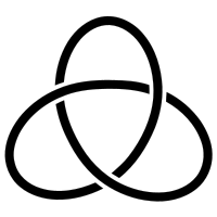
Figure 5: Trefoil knot(this figure courtesy of Wikipedia)

The algebraic knot in $S^{3}$ which is the main object in this section can be described by the intersection of $S^{3}$ with some algebraic curve. If we realize the sphere as

$$|z_{1}|^{2}+|z_{2}|^{2}=1$$ (83)

then the simplest $(p,q)$ torus knots which can be obtained from the unknot by the $SL(2,Z)$ action corresponds to the curve

$$z_{1}^{p}=z_{2}^{q}$$ (84)

which is called Seifert surface of the knot. The sphere is invariant under

$$z_{1}\rightarrow e^{i\theta}z_{1}\qquad z_{2}\rightarrow e^{i\theta}z_{2}$$ (85)

while the Seifert surface under

$$z_{1}\rightarrow e^{iq\theta}z_{1}\qquad z_{2}\rightarrow e^{ip\theta}z_{2}$$ (86)

In the CS theory the knot invariants one can evaluated from the corresponding Wilson loop vacuum expectation value. The useful tool is the knot operator introduced in [5]

$$W_{R}^{n,m}|p>=\sum_{\mu\in M_{R}}exp[-i\mu^{2}\frac{nm}{k+N}-2\pi i\frac{m}{k+N}p\mu]|p+n\mu>$$ (87)

where $M_{R}$ is the set of weights corresponding to the irreducible representation R and $|p>$ is the element of the basis of the Hilbert space of the SU(N) CS theory on the torus labeled by the weights p. When evaluating the vev of Wilson loop one performs the Heegaard cut of $S^{3}$ into two solid tori. Then the torus knot is introduced on the surface of one of the solid tori by the action of the knot operator on the corresponding vacuum state. In the standard framing the vev of Wilson loop is given by

$$<W^{n,m}_{R}>=E^{2\pi}\frac{<p|SW_{R}^{n,m}|p>}{<\rho|S|\rho>}$$ (88)

where S - is the operator of S-transformation from $SL(2,Z)$.

10 Appendix B. Higher (q,t) Catalan numbers

In this Appendix we briefly review higher (q,t) deformed Catalan numbers $C_{n}^{k}(q,t)$ which enter the expression for the $T_{n,nk+1}$ superpolynomial at $a=0$. There are several definitions of the higher Catalan numbers related to the geometry of the Hilbert schemes of points, symmetric functions, representation theory and combinatorics of paths. To orient the reader we provide a few of them

• Let us introduce the elementary symmetric functions $e_{n}$, Macdonald polynomial $H_{\mu}$ for the partition $\mu$, the Hall product $<.,.>$ on the symmetric functions and $\Lambda$ - the ring of the symmetric functions. There is the so-called Nabla operator $\nabla$ which act on the Macdonald basis as

  $$\nabla H_{\mu}=T_{\mu}H_{\mu},\qquad T_{\mu}=q^{n(\mu^{\prime}}t^{n(\mu)},\qquad n(\mu)=\sum_{x\in dg(\mu)}l(x)$$ (89)

  where $\mu^{\prime}$ denotes the transpose of $\mu$. The $C_{n}^{k}(q,t)$ in terms of the symmetric functions are defined as follows

  $$C_{n}^{k}(q,t)=<\nabla^{k}(e_{n}),e_{n}>$$ (90)

• One can define the higher Catalans in terms of the so-called diagonal harmonics. To this aim consider the polynomial ring $C(x_{1},y_{1},\dots,x_{n},y_{n})$ The symmetric group $S_{n}$ acts diagonally $\omega x_{i}=x_{\omega(i)}$ $\omega y_{i}=y_{\omega(i)}$ , $\omega\in S_{n}$. Introduce the ideal generated by all alternating polynomials and let be $\mathfrak{m}$ the maximal ideal generated by $x_{1},y_{i},\dots x_{n},y_{n}$ . Let $M^{k}=I^{k}/\mathfrak{m}I^{k}$. It is possible do introduce the double grading is the space of polynomials according the degrees in x and y variables. The grading tells that bi-degree $(d_{1},d_{2})$ corresponds to the situation when all monomials of the polynomial have equal bi-degree $(d_{1},d_{2})$. The higher Catalans are now defined as

  $$C_{n}^{k}(q,t)=\sum_{l}\sum_{s}q^{l}t^{s}dimM^{k}_{l,s}$$ (91)

  where $M^{k}_{l,s}$ is the bihomogeneous component of $M^{k}$ of bidegree (l,s).

• The last definition which is the closest to our context is based on the Hilbert scheme of n points on $C^{2}$ $Hilb^{n}(C^{2})$. Let us define $O(k)=O(1)^{\otimes k}$. where $O(1)=detT$ and T is the tautological rank n bundle. The double grading in this case is introduced on the set of global section $H^{0}(Z_{n},O(k))$ where $Z_{n}$ tells that all points are sitting at the top of each other. The $C_{n}^{k}(q,t)$ are now defined as follows

  $$C_{n}^{k}(q,t)=\sum_{l}\sum_{s}q^{l}t^{s}dimH^{0}(Z_{n},O(k))_{l,s}$$ (92)

Let us emphasize that the key property of the higher Catalans which is important in our study is that they provide the description of the properties of the set of points sitting at the top of each other.

11 Appendix C. The Dunkl operators and rational DAHA

In this Appendix we briefly describe the rational double affine Hecke algebras (DAHA) $H_{c}$ and their finite-dimensional representations relevant for the invariants of the torus knots. The rational DAHA of type $A_{n-1}$ with parameter c is generated by the $V=C^{n-1},V^{*}$ and the permutation group. $S_{n}$ with the following relations

$$\sigma x\sigma^{-1}=\sigma(x),\qquad\sigma y\sigma^{-1}=\sigma(y)$$ (93)

$$x_{1}x_{2}=x_{2}x_{1}\qquad y_{1}y_{2}=y_{2}y_{1}$$ (94)

$$yx-xy=<y,x>-c\sum_{s\in\mathfrak{S}}<\alpha_{s},x><y,\alpha_{s}^{v}>s$$ (95)

where $\mathfrak{S}$ is the set of all transpositions, and $\alpha_{s},\alpha_{s}^{v}$ are the corresponding roots and coroots.

It is convenient to introduce the Dunkl operators

$$D_{i}=\frac{\partial}{\partial x_{i}}-c\sum_{i\neq j}\frac{s_{ij}-1}{x_{i}-x_{j}}$$ (96)

and introduce the space of polynomial functions on V, where elements of V acts by the multiplications and $V^{*}$ by the Dunkl operators. This representation is denoted by $M_{c}$. It is known [79] that for rational $c=m/n$ DAHA has unique finite dimensional representation $L_{m/n}$ which was identified as the factor $L_{c}=M_{c}/I_{c}$ where $I_{c}$ is the ideal generated by the following set of the homogeneous polynomials $f_{i}$ of degree m

$$f_{i}=Coef_{m}[(1-zx_{i})^{-1}\prod_{i=1}^{n}(1-zx_{i})^{m/n}]$$ (97)

They are annihilated by the Dunkl operators

$$D_{k}(f_{i})=0$$ (98)

and therefore are invariants under the DAHA action. The dimension of the finite-dimensional representation is

$$dimL^{m/n}=m^{n-1}$$ (99)

There is $SL(2,R)$ subalgebra of DAHA which involves the Hamiltonian of the rational complexified Calogero model

$$H_{Cal}=\sum_{i}D_{i}^{2}$$ (100)

the rest of the operators from this subalgebra are

$$K=\frac{1}{2}\sum_{i}(x_{i}D_{i}+D_{i}x_{i})\qquad J_{1}=\sum_{i}x_{i}^{2}$$ (101)

Let us also note that there is the so-called shift operator which acts by changing $c\rightarrow c+1$ and is the counterpart of the Nabla operator in the theory of the symmetric functions and the cut- and-join operator. It corresponds to the shift of the level of 5d CS term.

12 Appendix D. The Ruijsenaars-Shneyder many-body integrable model from the perturbed CS theory

The surface operator which survives at the road from UV to IR [30] induces the action of the quantum trigonometric RS Hamiltonian which is simply described in terms o the perturbed 3d CS theory [51]. The phase space in this model is identified with the space of flat connections on the torus with the marked point and particular monodromy around while the Hamiltonian can be described as the Wilson loop around one cycle.

Equivalently is can be obtained via the Hamiltonian reduction. To perform the Hamiltonian reduction replace the space of two dimensional gauge fields by the cotangent space to the loop group:

$$T^{*}\hat{G}=\{(g(x),k_{x}+P(x))\}$$

The relation to the two dimensional construction is the following. Choose a non-contractible circle $\bf S^{1}$ on the two-torus which does not pass through the marked point $p$. Let $x,y$ be the coordinates on the torus and $y=0$ is the equation of the $\bf S^{1}$. The periodicity of $x$ is $\beta$ and that of $y$ is $R$. Then

$$P(x)=A_{x}(x,0),g(x)=P\exp\int_{0}^{R}A_{y}(x,y)dy.$$

The moment map equation looks as follows:

$$kg^{-1}_{x}g+g^{-1}Pg-P=J\delta(x),$$ (102)

with $k={1\over{R\beta}}$. The solution of this equation in the gauge $P={\rm diag}(q_{1},\ldots,q_{N})$ leads to the Lax operator $A=g(0)$ with $R,\beta$ exchanged. On the other hand, if we diagonalize $g(x)$:

$$g(x)={\rm diag}\left(z_{1}=e^{{\sqrt{-}1}Rq_{1}},\ldots,z_{N}=e^{{\sqrt{-}1}Rq_{N}}\right)$$ (103)

then a similar calculation leads to the Lax operator

$$B=P\exp\oint{1\over{k}}P(x)dx={\rm diag}(e^{{\sqrt{-}1}\theta_{i}})\exp{\sqrt{-}1}R\beta\nu{\rm r}$$

with

$${\rm r}_{ij}={1\over{1-e^{{\sqrt{-}1}Rq_{ji}}}},i\neq j;\quad{\rm r}_{ii}=-\sum_{j\neq i}{\rm r}_{ij}$$

thereby establishing the duality $A\leftrightarrow B$ explicitly.

References

- [1] Edward Witten “Quantum Field Theory and the Jones Polynomial” In Commun.Math.Phys. 121, 1989, pp. 351–399 DOI: 10.1007/BF01217730
- [2] Hirosi Ooguri and Cumrun Vafa “Knot invariants and topological strings” In Nucl.Phys. B577, 2000, pp. 419–438 DOI: 10.1016/S0550-3213(00)00118-8
- [3] Andrea Brini, Bertrand Eynard and Marcos Marino “Torus knots and mirror symmetry” In Annales Henri Poincare 13, 2012, pp. 1873–1910 DOI: 10.1007/s00023-012-0171-2
- [4] Hans Jockers, Albrecht Klemm and Masoud Soroush “Torus Knots and the Topological Vertex” In Lett.Math.Phys. 104, 2014, pp. 953–989 DOI: 10.1007/s11005-014-0687-0
- [5] J. M. F. Labastida and Marcos Marino “Polynomial invariants for torus knots and topological strings” In Commun. Math. Phys. 217, 2001, pp. 423–449 DOI: 10.1007/s002200100374
- [6] Sergei Gukov, Albert S. Schwarz and Cumrun Vafa “Khovanov-Rozansky homology and topological strings” In Lett.Math.Phys. 74, 2005, pp. 53–74 DOI: 10.1007/s11005-005-0008-8
- [7] Nathan M. Dunfield, Sergei Gukov and Jacob Rasmussen “The Superpolynomial for knot homologies”, 2005 arXiv:math/0505662 [math.GT]
- [8] Edward Witten “Fivebranes and Knots”, 2011 arXiv:1101.3216 [hep-th]
- [9] Davide Gaiotto and Edward Witten “Knot Invariants from Four-Dimensional Gauge Theory” In Adv.Theor.Math.Phys. 16.3, 2012, pp. 935–1086 DOI: 10.4310/ATMP.2012.v16.n3.a5
- [10] Mina Aganagic and Shamil Shakirov “Knot Homology and Refined Chern-Simons Index” In Commun.Math.Phys. 333.1, 2015, pp. 187–228 DOI: 10.1007/s00220-014-2197-4
- [11] Tudor Dimofte, Davide Gaiotto and Sergei Gukov “Gauge Theories Labelled by Three-Manifolds” In Commun.Math.Phys. 325, 2014, pp. 367–419 DOI: 10.1007/s00220-013-1863-2
- [12] Hiroyuki Fuji, Sergei Gukov and Piotr Sulkowski “Super-A-polynomial for knots and BPS states” In Nucl. Phys. B867, 2013, pp. 506–546 DOI: 10.1016/j.nuclphysb.2012.10.005
- [13] Mathew Bullimore, Martin Fluder, Lotte Hollands and Paul Richmond “The superconformal index and an elliptic algebra of surface defects” In JHEP 10, 2014, pp. 62 DOI: 10.1007/JHEP10(2014)062
- [14] N. Dorey “The BPS spectra of two-dimensional supersymmetric gauge theories with twisted mass terms” In JHEP 11, 1998, pp. 005 arXiv:hep-th/9806056 [hep-th]
- [15] Mina Aganagic, Nathan Haouzi and Shamil Shakirov “-Triality”, 2014 arXiv:1403.3657 [hep-th]
- [16] Mina Aganagic and Cumrun Vafa “Large N Duality, Mirror Symmetry, and a Q-deformed A-polynomial for Knots”, 2012 arXiv:1204.4709 [hep-th]
- [17] Yuji Terashima and Masahito Yamazaki “SL(2,R) Chern-Simons, Liouville, and Gauge Theory on Duality Walls” In JHEP 08, 2011, pp. 135 DOI: 10.1007/JHEP08(2011)135
- [18] Abhijit Gadde, Sergei Gukov and Pavel Putrov “Walls, Lines, and Spectral Dualities in 3d Gauge Theories” In JHEP 1405, 2014, pp. 047 DOI: 10.1007/JHEP05(2014)047
- [19] Sergei Gukov and Ingmar Saberi “Lectures on Knot Homology and Quantum Curves”, 2012 arXiv:1211.6075 [hep-th]
- [20] Alexei Oblomkov and Vivek Shende “The Hilbert scheme of a plane curve singularity and the HOMFLY polynomial of its link” In Duke Math. J. 161.7 Duke University Press, 2012, pp. 1277–1303 DOI: 10.1215/00127094-1593281
- [21] Eugene Gorsky, Alexei Oblomkov, Jacob Rasmussen and Vivek Shende “Torus knots and the rational DAHA” In Duke Math. J. 163.14 Duke University Press, 2014, pp. 2709–2794 DOI: 10.1215/00127094-2827126
- [22] E Gorsky “q, t-Catalan numbers and knot homology” In Zeta functions in algebra and geometry, 2012, pp. 213–232 arXiv:1003.0916
- [23] E. Gorsky and A. Neguţ “Refined knot invariants and Hilbert schemes” In ArXiv e-prints, 2013 arXiv:1304.3328 [math.RT]
- [24] A. Losev, N. Nekrasov and Samson L. Shatashvili “Issues in topological gauge theory” In Nucl. Phys. B534, 1998, pp. 549–611 DOI: 10.1016/S0550-3213(98)00628-2
- [25] Gregory W. Moore, Nikita Nekrasov and Samson Shatashvili “Integrating over Higgs branches” In Commun. Math. Phys. 209, 2000, pp. 97–121 DOI: 10.1007/PL00005525
- [26] A. Losev, N. Nekrasov and Samson L. Shatashvili “Freckled instantons in two-dimensions and four-dimensions” In Strings ’99. Proceedings, Conference, Potsdam, Germany, July 19-24, 1999 17, 2000, pp. 1181–1187 DOI: 10.1088/0264-9381/17/5/327
- [27] Nikita Nekrasov and Albert S. Schwarz “Instantons on noncommutative R**4 and (2,0) superconformal six-dimensional theory” In Commun. Math. Phys. 198, 1998, pp. 689–703 DOI: 10.1007/s002200050490
- [28] Harry W. Braden and Nikita A. Nekrasov “Space-time foam from noncommutative instantons” In Commun. Math. Phys. 249, 2004, pp. 431–448 DOI: 10.1007/s00220-004-1127-2
- [29] N. Nekrasov “Non-Perturbative Schwinger–Dyson Equations: From BPS/CFT Correspondence to the Novel Symmetries of Quantum Field Theory” Gorsky, Alexander(ed.) and Vysotsky, Mikhail(ed.), Proceedings, 100th anniversary of the birth of I.Ya. Pomeranchuk (Pomeranchuk 100), 2014 DOI: 10.1142/9242
- [30] Davide Gaiotto, Leonardo Rastelli and Shlomo S. Razamat “Bootstrapping the superconformal index with surface defects” In JHEP 1301, 2013, pp. 022 DOI: 10.1007/JHEP01(2013)022
- [31] Shlomo S. Razamat and Brian Willett “Down the rabbit hole with theories of class ” In JHEP 10, 2014, pp. 99 DOI: 10.1007/JHEP10(2014)099
- [32] Nikita A. Nekrasov “Seiberg-Witten prepotential from instanton counting” In Adv.Theor.Math.Phys. 7, 2004, pp. 831–864 DOI: 10.4310/ATMP.2003.v7.n5.a4
- [33] Alexandr Gorsky “Angular Momentum and Gravimagnetization of the SYM vacuum” In Theor. Math. Phys. 171, 2012, pp. 616–628 DOI: 10.1007/s11232-012-0059-9
- [34] K. Bulycheva, A. Gorsky and S. Nechaev “Critical behavior in topological ensembles”, 2014 arXiv:1409.3350 [hep-th]
- [35] Nikita Nekrasov and Andrei Okounkov “Seiberg-Witten theory and random partitions”, 2003 arXiv:hep-th/0306238 [hep-th]
- [36] Albion E. Lawrence and Nikita Nekrasov “Instanton sums and five-dimensional gauge theories” In Nucl.Phys. B513, 1998, pp. 239–265 DOI: 10.1016/S0550-3213(97)00694-9
- [37] A.M. Garsia and M. Haiman “A Remarkable q, t-Catalan Sequence and q-Lagrange Inversion” In Journal of Algebraic Combinatorics 5.3 Kluwer Academic Publishers-Plenum Publishers, 1996, pp. 191–244 DOI: 10.1023/A:1022476211638
- [38] Mark Haiman “t, q-Catalan numbers and the Hilbert scheme” In Discrete Mathematics 193.1 Elsevier, 1998, pp. 201–224
- [39] Amer Iqbal, Can Kozcaz and Cumrun Vafa “The Refined topological vertex” In JHEP 0910, 2009, pp. 069 DOI: 10.1088/1126-6708/2009/10/069
- [40] Amer Iqbal, Can Kozcaz and Khurram Shabbir “Refined Topological Vertex, Cylindric Partitions and the U(1) Adjoint Theory” In Nucl.Phys. B838, 2010, pp. 422–457 DOI: 10.1016/j.nuclphysb.2010.06.010
- [41] Kenneth A. Intriligator, David R. Morrison and Nathan Seiberg “Five-dimensional supersymmetric gauge theories and degenerations of Calabi-Yau spaces” In Nucl.Phys. B497, 1997, pp. 56–100 DOI: 10.1016/S0550-3213(97)00279-4
- [42] Albrecht Klemm and Piotr Sulkowski “Seiberg-Witten theory and matrix models” In Nucl.Phys. B819, 2009, pp. 400–430 DOI: 10.1016/j.nuclphysb.2009.04.004
- [43] Ksenia Bulycheva and Alexander Gorsky “BPS states in the Omega-background and torus knots” In JHEP 1404, 2014, pp. 164 DOI: 10.1007/JHEP04(2014)164
- [44] Andrea Brini, Bertrand Eynard and Marcos Marino “Torus knots and mirror symmetry” In Annales Henri Poincare 13, 2012, pp. 1873–1910 DOI: 10.1007/s00023-012-0171-2
- [45] Neil D. Lambert and David Tong “Dyonic instantons in five-dimensional gauge theories” In Phys. Lett. B462, 1999, pp. 89–94 DOI: 10.1016/S0370-2693(99)00894-1
- [46] Heng-Yu Chen, Minoru Eto and Koji Hashimoto “The Shape of Instantons: Cross-Section of Supertubes and Dyonic Instantons” In JHEP 01, 2007, pp. 017 DOI: 10.1088/1126-6708/2007/01/017
- [47] Roy P Kerr “Gravitational field of a spinning mass as an example of algebraically special metrics” In Physical review letters 11.5 APS, 1963, pp. 237
- [48] Edward Witten “BPS Bound states of D0 - D6 and D0 - D8 systems in a B field” In JHEP 04, 2002, pp. 012 DOI: 10.1088/1126-6708/2002/04/012
- [49] M. Shifman and A. Yung “Supersymmetric Solitons and How They Help Us Understand Non-Abelian Gauge Theories” In Rev. Mod. Phys. 79, 2007, pp. 1139 DOI: 10.1103/RevModPhys.79.1139
- [50] Minoru Eto, Muneto Nitta, Keisuke Ohashi and David Tong “Skyrmions from instantons inside domain walls” In Phys. Rev. Lett. 95, 2005, pp. 252003 DOI: 10.1103/PhysRevLett.95.252003
- [51] Alexander Gorsky and Nikita Nekrasov “Relativistic Calogero-Moser model as gauged WZW theory” In Nucl. Phys. B436, 1995, pp. 582–608 DOI: 10.1016/0550-3213(94)00499-5
- [52] V.A. Novikov, Mikhail A. Shifman, A.I. Vainshtein and Valentin I. Zakharov “Instanton Effects in Supersymmetric Theories” In Nucl.Phys. B229, 1983, pp. 407 DOI: 10.1016/0550-3213(83)90340-1
- [53] Alexander A. Migdal “Loop Equations and 1/N Expansion” In Phys. Rept. 102, 1983, pp. 199–290 DOI: 10.1016/0370-1573(83)90076-5
- [54] Alexander M. Polyakov “Gauge Fields as Rings of Glue” In Nucl. Phys. B164, 1980, pp. 171–188 DOI: 10.1016/0550-3213(80)90507-6
- [55] Mikhail A. Shifman “Anomalies and Low-Energy Theorems of Quantum Chromodynamics” [Usp. Fiz. Nauk157,561(1989)] In Phys. Rept. 209, 1991, pp. 341–378 DOI: 10.1016/0370-1573(91)90020-M
- [56] A. Gorsky, M. Shifman and A. Yung “Non-Abelian meissner effect in Yang-Mills theories at weak coupling” In Phys. Rev. D71, 2005, pp. 045010 DOI: 10.1103/PhysRevD.71.045010
- [57] Edward Witten “Instantons, the Quark Model, and the 1/n Expansion” In Nucl. Phys. B149, 1979, pp. 285 DOI: 10.1016/0550-3213(79)90243-8
- [58] V. P. Gusynin, V. A. Miransky and I. A. Shovkovy “Dimensional reduction and catalysis of dynamical symmetry breaking by a magnetic field” In Nucl. Phys. B462, 1996, pp. 249–290 DOI: 10.1016/0550-3213(96)00021-1
- [59] Eugene Gorsky, Alexei Oblomkov and Jacob Rasmussen “On stable Khovanov homology of torus knots” In Experimental Mathematics 22.3 Taylor & Francis, 2013, pp. 265–281
- [60] P. Dunin-Barkowski et al. “Superpolynomials for toric knots from evolution induced by cut-and-join operators” In JHEP 1303, 2013, pp. 021 DOI: 10.1007/JHEP03(2013)021
- [61] K. Bulycheva, A. Gorsky, A. Milekhin and S. Nechaev, in preparation
- [62] Edward Witten “Phase transitions in M theory and F theory” In Nucl.Phys. B471, 1996, pp. 195–216 DOI: 10.1016/0550-3213(96)00212-X
- [63] Yuji Tachikawa “Five-dimensional Chern-Simons terms and Nekrasov’s instanton counting” In JHEP 02, 2004, pp. 050 DOI: 10.1088/1126-6708/2004/02/050
- [64] Alexander Gorsky “SQCD, Superconducting Gaps and Cyclic RG Flows”, 2012 arXiv:1202.4306 [hep-th]
- [65] Oleg Dubinkin “On the Virasoro constraints for torus knots” In J.Phys. A47.48, 2014, pp. 485203 DOI: 10.1088/1751-8113/47/48/485203
- [66] Luis F. Alday, Davide Gaiotto and Yuji Tachikawa “Liouville Correlation Functions from Four-dimensional Gauge Theories” In Lett.Math.Phys. 91, 2010, pp. 167–197 DOI: 10.1007/s11005-010-0369-5
- [67] A. Gorsky, S. Gukov and A. Mironov “Multiscale N=2 SUSY field theories, integrable systems and their stringy / brane origin. 1.” In Nucl. Phys. B517, 1998, pp. 409–461 DOI: 10.1016/S0550-3213(98)00055-8
- [68] A. Gorsky, S. Gukov and A. Mironov “SUSY field theories, integrable systems and their stringy / brane origin. 2.” In Nucl. Phys. B518, 1998, pp. 689–713 DOI: 10.1016/S0550-3213(98)00106-0
- [69] Ling Bao, Elli Pomoni, Masato Taki and Futoshi Yagi “M5-Branes, Toric Diagrams and Gauge Theory Duality” In JHEP 1204, 2012, pp. 105 DOI: 10.1007/JHEP04(2012)105
- [70] Alexander B. Zamolodchikov and Alexei B. Zamolodchikov “Structure constants and conformal bootstrap in Liouville field theory” In Nucl. Phys. B477, 1996, pp. 577–605 DOI: 10.1016/0550-3213(96)00351-3
- [71] Harald Dorn and H. J. Otto “Two and three point functions in Liouville theory” In Nucl. Phys. B429, 1994, pp. 375–388 DOI: 10.1016/0550-3213(94)00352-1
- [72] Hidetoshi Awata and Yasuhiko Yamada “Five-dimensional AGT Conjecture and the Deformed Virasoro Algebra” In JHEP 1001, 2010, pp. 125 DOI: 10.1007/JHEP01(2010)125
- [73] Can Kozcaz, Sara Pasquetti and Niclas Wyllard “A and B model approaches to surface operators and Toda theories” In JHEP 1008, 2010, pp. 042 DOI: 10.1007/JHEP08(2010)042
- [74] Ricardo Schiappa and Niclas Wyllard “An A(r) threesome: Matrix models, 2d CFTs and 4d N=2 gauge theories” In J.Math.Phys. 51, 2010, pp. 082304 DOI: 10.1063/1.3449328
- [75] Nikita A. Nekrasov and Samson L. Shatashvili “Supersymmetric vacua and Bethe ansatz” In Cargese 2008, theory and particle physics : The LHC perspective and beyond, proceedings of the ESF School in High Energy Physics and Astrophysics, Cargese Summer School, Cargese, France, 16-28 June 2008 192-193, 2009, pp. 91–112 DOI: 10.1016/j.nuclphysbps.2009.07.047
- [76] N. Nekrasov “Supersymmetric gauge theories and quantization of integrable systems” In Strings 2009, 2009
- [77] Evgeny Gorsky “Arc spaces and DAHA representations” In Selecta Mathematica 19.1 Springer, 2013, pp. 125–140 arXiv:1110.1674
- [78] Ivan Cherednik “A unification of Knizhnik-Zamolodchikov and Dunkl operators via affine Hecke algebras” In Inventiones mathematicae 106.1 Springer, 1991, pp. 411–431
- [79] Yuri Berest, Pavel Etingof and Victor Ginzburg “Finite dimensional representations of rational Cherednik algebras” In arXiv preprint math/0208138, 2002
- [80] Benjamin Collie and David Tong “Instantons, Fermions and Chern-Simons Terms” In JHEP 07, 2008, pp. 015 DOI: 10.1088/1126-6708/2008/07/015
- [81] Seok Kim, Ki-Myeong Lee and Sungjay Lee “Dyonic Instantons in 5-dim Yang-Mills Chern-Simons Theories” In JHEP 08, 2008, pp. 064 DOI: 10.1088/1126-6708/2008/08/064
- [82] Leonard Susskind “The Quantum Hall fluid and noncommutative Chern-Simons theory”, 2001 arXiv:hep-th/0101029 [hep-th]
- [83] Alexios P. Polychronakos “Quantum Hall states on the cylinder as unitary matrix Chern-Simons theory” In JHEP 06, 2001, pp. 070 DOI: 10.1088/1126-6708/2001/06/070
- [84] A. Gorsky, I. I. Kogan and C. Korthels-Altes “Dualities in quantum Hall system and noncommutative Chern-Simons theory” In JHEP 01, 2002, pp. 002 DOI: 10.1088/1126-6708/2002/01/002
- [85] M. Shifman and A. Yung “Lessons from supersymmetry: ”Instead-of-Confinement” Mechanism” In Int. J. Mod. Phys. A29.27, 2014, pp. 1430064 DOI: 10.1142/S0217751X14300646
- [86] A. Gorsky, M. Shifman and A. Yung “Revisiting the Faddeev-Skyrme Model and Hopf Solitons” In Phys.Rev. D88, 2013, pp. 045026 DOI: 10.1103/PhysRevD.88.045026
- [87] S. Bolognesi “Instanton Bags, High Density Holographic QCD and Chiral Symmetry Restoration” In Phys. Rev. D90.10, 2014, pp. 105015 DOI: 10.1103/PhysRevD.90.105015
- [88] Sergei Gukov and Marko Stošić “Homological Algebra of Knots and BPS States” In Proceedings, String-Math 2011 85, 2012, pp. 125–172 DOI: 10.1090/pspum/085/1377
- [89] Eugene Gorsky, Sergei Gukov and Marko Stosic “Quadruply-graded colored homology of knots”, 2013 arXiv:1304.3481 [math.QA]
- [90] Jiang-ping Hu and Shou-Cheng Zhang “Collective excitations at the boundary of a 4-D quantum Hall droplet” In Phys. Rev. B66, 2002, pp. 125301 DOI: 10.1103/PhysRevB.66.125301
- [91] K. M. Bulycheva and A. S. Gorsky “Limit cycles in renormalization group dynamics” In Proceedings, 100th anniversary of the birth of I.Ya. Pomeranchuk 57, 2014, pp. 171–182 DOI: 10.3367/UFNe.0184.201402g.0182
- [92] Alexander Givental and Bum-sig Kim “Quantum cohomology of flag manifolds and Toda lattices” In Commun. Math. Phys. 168, 1995, pp. 609–642 DOI: 10.1007/BF02101846
- [93] Davide Gaiotto and Peter Koroteev “On Three Dimensional Quiver Gauge Theories and Integrability” In JHEP 1305, 2013, pp. 126 DOI: 10.1007/JHEP05(2013)126
- [94] A. Gorsky, A. Zabrodin and A. Zotov “Spectrum of Quantum Transfer Matrices via Classical Many-Body Systems” In JHEP 01, 2014, pp. 070 DOI: 10.1007/JHEP01(2014)070
- [95] Eugene Gorsky, Sergei Gukov and Marko Stosic “Quadruply-graded colored homology of knots”, 2013 arXiv:1304.3481 [math.QA]
- [96] M. Shifman and A. Yung “Quantum Deformation of the Effective Theory on Non-Abelian string and 2D-4D correspondence” In Phys. Rev. D89.6, 2014, pp. 065035 DOI: 10.1103/PhysRevD.89.065035
- [97] Louis H Kauffman “Knots and physics” World scientific, 2013
- [98] William P Thurston “Three-dimensional manifolds, Kleinian groups and hyperbolic geometry” In Proc. Sympos. Pure Math 39, 1983, pp. 87–111