On the generalized shift-splitting preconditioner for saddle point problems

Abstract. In this paper, the generalized shift-splitting preconditioner is implemented for saddle point problems with symmetric positive definite (1,1)-block and symmetric positive semidefinite (2,2)-block. The proposed preconditioner is extracted form a stationary iterative method which is unconditionally convergent. Moreover, a relaxed version of the proposed preconditioner is presented and some properties of the eigenvalues distribution of the corresponding preconditioned matrix are studied. Finally, some numerical experiments on test problems arisen from finite element discretization of the Stokes problem are given to show the effectiveness of the preconditioners.

Keywords: Saddle point problem, preconditioner, shift-splitting, symmetric positive definite.
AMS Subject Classification: 65F10, 65F50, 65N22.

1 Introduction

Consider the saddle point linear system

$$\mathcal{A}u\equiv\left(\begin{array}[]{cc}A&B^{T}\\ -B&C\end{array}\right)\left(\begin{array}[]{c}x\\ y\end{array}\right)=\left(\begin{array}[]{c}f\\ -g\end{array}\right)\equiv b,$$ (1)

where $A\in\mathbb{R}^{n\times n}$ is symmetric positive definite (SPD), $C\in\mathbb{R}^{m\times m}$ is symmetric positive semidefinite and $B\in\mathbb{R}^{m\times n}$, $m\leq n$, is of full rank. Moreover, $x,f\in\mathbb{R}^{n}$ and $y,g\in\mathbb{R}^{m}$. We also assume that the matrices $A$, $B$ and $C$ are large and sparse. According to Lemma 1.1 in [9] the matrix $\mathcal{A}$ is nonsingular. Such systems arise in a variety of scientific computing and engineering applications, including constrained optimization, computational fluid dynamics, mixed finite element discretization of the Navier-Stokes equations, etc. (see [1, 10, 14, 25]). Application-based analysis can be seen in [22, 26, 28].

In the last decade, there has been intensive work on development of the effective iterative methods for solving matrix equations with different structures (see for example [4, 18, 19, 20, 21, 27]). Benzi and Golub [9] investigated the convergence and the preconditioning properties of the Hermitian and skew-Hermitian splitting (HSS) iterative method [4], when it is used for solving the saddle point problems. Bai et al. in [5] established the preconditioned HSS (PHSS) iterative method, which involves a single parameter, and then, Bai and Golub in [3] proposed its two-parameter acceleration, called the accelerated Hermitian and skew-Hermitian splitting (AHSS) iterative method; see also [2]. Besides these HSS methods, Uzawa-type schemes [6, 7, 13, 16, 23] and preconditioned Krylov subspace methods, such as MINRES and GMRES incorporated with suitable preconditioners have also been applied to solve the saddle point problems (see [29, 30, 31, 32] and the references therein as well as [11, 12]). The reader is also referred to [10] for a comprehensive survey.

To solve the saddle point problem (1) when $C=0$, Cao et al., in [15], proposed the shift-splitting preconditioner

$$\mathcal{P}_{SS}=\frac{1}{2}(\alpha I+\mathcal{A})=\frac{1}{2}\left(\begin{array}[]{cc}\alpha I+A&B^{T}\\ -B&\alpha I\\ \end{array}\right),$$

which is a skillful generalization of the idea of the shift-splitting preconditioner initially introduced in [8] for solving a non-Hermitian positive definite linear system where $\alpha>0$ and $I$ is the identity matrix. Recently, Chen and Ma in [17] studied the two-parameter generalization of the preconditioner $\mathcal{P}_{SS}$, say

$$\mathcal{P}_{GSS}=\frac{1}{2}\left(\begin{array}[]{cc}\alpha I+A&B^{T}\\ -B&\beta I\\ \end{array}\right),$$

for solving the saddle point linear systems (1) with $C=0$, where $\alpha\geq 0$ and $\beta>0$.

In this paper, we propose a modified generalized shift-splitting (MGSS) preconditioner for the saddle point problem (1) with $C\neq 0$. The MGSS preconditioner is based on a splitting of the saddle point matrix which results in an unconditionally convergent stationary iterative method. Moreover, a relaxed version of the MGSS preconditioner is presented and the eigenvalues distribution of the corresponding preconditioned matrix is studied.

The organization of the paper is as follows. In Section 2 we propose the MGSS preconditioner and its relaxed version. Section 3 is devoted to some numerical experiments. Finally, in Section 4 we present some concluding remarks.

2 The generalized shift-splitting preconditioner

Let $\alpha,\beta>0$. Consider the splitting $\mathcal{A}=\mathcal{M}_{\alpha,\beta}-\mathcal{N}_{\alpha,\beta}$, where

$$\mathcal{M}_{\alpha,\beta}=\frac{1}{2}\left({\begin{array}[]{*{20}{c}}\alpha I+A&B^{T}\\ -B&\beta I+C\end{array}}\right)\quad\textrm{and}\quad\mathcal{N}_{\alpha,\beta}=\frac{1}{2}\left({\begin{array}[]{*{20}{c}}\alpha I-A&-B^{T}\\ B&\beta I-C\end{array}}\right).$$ (2)

This splitting leads to the following stationary iterative method (the MGSS iterative scheme) (1)

$$\mathcal{M}_{\alpha,\beta}u^{(k+1)}=\mathcal{N}_{\alpha,\beta}u^{(k)}+b$$ (3)

for solving the linear system (1), where $u^{(0)}$ is an initial guess. Therefore, the iteration matrix of the MGSS iterative method is given by $\Gamma_{\alpha,\beta}=\mathcal{M}_{\alpha,\beta}^{-1}\mathcal{N}_{\alpha,\beta}$. In the sequel, the convergence of the proposed method is studied. It is well known that the iterative method (3) is convergent for every initial guess $u^{(0)}$ if and only if $\rho(\Gamma_{\alpha,\beta})<1$, where $\rho(.)$ denotes the spectral radius of $\Gamma$ (see [1]). Let $u=(x;y)$ be an eigenvector corresponding to the eigenvalue $\lambda$ of $\Gamma_{\alpha,\beta}$. Then, we have $\mathcal{N}_{\alpha,\beta}u=\lambda\mathcal{M}_{\alpha,\beta}u$ or equivalently

$$(\alpha I-A)x-B^{T}y = \lambda(\alpha I+A)x+\lambda B^{T}y,$$ (4)

$$Bx+(\beta I-C)y = -\lambda Bx+\lambda(\beta I+C)y.$$ (5)

Lemma 1.

Let $\alpha,\beta>0$. If $\lambda$ is an eigenvalue of the matrix $\Gamma_{\alpha,\beta}$, then $\lambda\neq\pm 1$.

Proof.

If $\lambda=1$, then from Eqs. (4) and (5) we obtain $\mathcal{A}u=0$ which is a contradiction, since $u\neq 0$ and the matrix $\mathcal{A}$ is nonsingular ([9, Lemma 1.1]).

If $\lambda=-1$, then from Eqs. (4) and (5) it follows that $2\alpha x=0$ and $2\beta x=0$. Since, $\alpha,\beta>0$, we get $x=0$ and $y=0$. This is a contradiction, because $(x;y)$ is an eigenvector of $\mathcal{A}$. ∎

Theorem 1.

Let $\lambda$ be an eigenvalue of the matrix $\Gamma$ and $\alpha,\beta>0$. Then $|{\lambda}|<1$.

Proof.

We first show that $x\neq 0$. If $x=0$, then it follows from Eq. (4) that $(1+\lambda)B^{T}y=0$. Therefore, from Lemma 1 we conclude that $B^{T}y=0$ and this yields $y=0$, since $B$ has full rank. This is a contradiction because $(x;y)$ is an eigenvector of $\Gamma_{\alpha,\beta}$.

Without loss of generality let ${\left\|{x}\right\|}_{2}=1$. Multiplying both sides of (4) by $x^{*}$ yields

$$\alpha-x^{*}Ax-(Bx)^{*}y=\lambda(\alpha{\left\|{x}\right\|}_{2}^{2}+x^{*}Ax)+\lambda(Bx)^{*}y.$$ (6)

We consider two cases $Bx=0$ and $Bx\neq 0$. If $Bx=0$, then Eq. (6) implies

$$|\lambda|=\frac{|\alpha-x^{*}Ax|}{|\alpha+x^{*}Ax|}<1.$$

We now assume that $Bx\neq 0$. In this case, from Eq. (5) we obtain

$$Bx=\frac{\beta(\lambda-1)}{\lambda+1}y+Cy.$$ (7)

Substituting Eq. (7) in (6) yields

$$(1-\lambda)\alpha-(1+\lambda)x^{*}Ax=(1+\lambda)\left(\beta\frac{\overline{\lambda}-1}{1+\overline{\lambda}}y^{*}y+y^{*}Cy\right).$$

Letting $p=x^{*}Ax$, $q=y^{*}y$, and $r=y^{*}Cy$, it follows from the latter equation that

$$\alpha\omega+\beta q\overline{\omega}=p+r,\quad\textrm{with}\quad\omega=\frac{1-\lambda}{1+\lambda}.$$ (8)

Since $\alpha,\beta,p>0$ and $q,r\geq 0$, form (8) we see that

$$\Re(w)=\frac{p+r}{\alpha+\beta q}>0.$$

Hence, we have

$$|\lambda|=\frac{|1-\omega|}{|1+\omega|}=\sqrt{\frac{(1-\Re(\omega))^{2}+\Im(\omega)^{2}}{(1+\Re(\omega))^{2}+\Im(\omega)^{2}}}<1$$

which completes the proof. ∎

Remark 1.

Let $C=0$. If $\alpha=\beta>0$ then MGSS iterative method is reduced to the shift-splitting method presented by Cao et al. in [15] and when $\alpha$ and $\beta$ are two positive parameters the method becomes the generalized shif-splitting method proposed by Chen and Ma in [17].

Theorem 1 guarantees the convergence of the MGSS method, however the stationary iterative method (3) is typically too slow for the method to be competitive. Nevertheless, it serves the preconditioner $\mathcal{P}_{MGSS}=\mathcal{M}_{\alpha,\beta}$ for a Krylov subspace method such as GMRES, or its restarted version GMRES($m$) to solve system (1). At each step of the MGSS iterative method or applying the shift-splitting preconditioner $\mathcal{P}_{MGSS}$ within a Krylov subspace method, we need to compute a vector of the form $z=\mathcal{P}_{MGSS}^{-1}r$ for a given $r=(r_{1};r_{2})$ where $r_{1}\in\mathbb{R}^{n}$ and $r_{2}\in\mathbb{R}^{m}$. It is not difficult to check that

$$\mathcal{P}_{MGSS} =\frac{1}{2}\left({\begin{array}[]{*{20}{c}}I&B^{T}\left(\beta I+C\right)^{-1}\\ 0&I\end{array}}\right)\left({\begin{array}[]{*{20}{c}}S&0\\ 0&\beta I+C\end{array}}\right)\left({\begin{array}[]{*{20}{c}}I&0\\ -\left(\beta I+C\right)^{-1}B&I\end{array}}\right),$$

where $S=\alpha I+A+B^{T}\left(\beta I+C\right)^{-1}B$. Hence,

$$\mathcal{P}_{MGSS}^{-1} =2\left({\begin{array}[]{*{20}{c}}I&0\\ \left(\beta I+C\right)^{-1}B&I\end{array}}\right)\left({\begin{array}[]{*{20}{c}}S^{-1}&0\\ 0&(\beta I+C)^{-1}\end{array}}\right)\left({\begin{array}[]{*{20}{c}}I&-B^{T}\left(\beta I+C\right)^{-1}\\ 0&I\end{array}}\right).$$ (15)

By using Eq. (15) we state Algorithm 1 to compute the vector $z=(z_{1};z_{2})$ where $z_{1}\in\mathbb{R}^{n}$ and $z_{2}\in\mathbb{R}^{m}$ as following.

Algorithm 1.

Computation of $z=\mathcal{P}_{MGSS}^{-1}r$.

1. Solve $(\beta I+C)w=2r_{2}$ for $w$.
   

2. Compute $w_{1}=2r_{1}-B^{T}w$.
   

3. Solve $\left(\alpha I+A+B^{T}(\beta I+C)^{-1}B\right)z_{1}=w_{1}$ for $z_{1}$.
   

4. Solve $(\beta I+C)v=Bz_{1}$ for $v$.
   

5. Compute $z_{2}=v+w$.

Obviously, the matrix $S=\alpha I+A+B^{T}(\beta I+C)^{-1}B$ is SPD. In practical implementation of Algorithm 1 one may use the conjugate gradient (CG) method or a preconditioned CG (PCG) method to solve the system of Step 3. It is noted that, since the matrix $\beta I+C$ is SPD and of small size in comparison to the size of $A$, we use the Cholesky factorization of $\beta I+C$ in Steps 1, 3 and 4.

In the sequel, we consider the relaxed MGSS (RMGSS) preconditioner

$$\mathcal{P}_{RMGSS}=\left({\begin{array}[]{*{20}{c}}A&B^{T}\\ -B&\beta I+C\end{array}}\right).$$

for the saddle point problem (1). The next theorem discusses eigenvalues distribution of $\mathcal{P}_{RMGSS}^{-1}\mathcal{A}$.

Theorem 2.

The preconditioned matrix $\Psi=\mathcal{P}_{RMGSS}^{-1}\mathcal{A}$ has an eigenvalue 1 with multiplicity $n$ and the remaining eigenvalues are $\lambda_{i}=\frac{\mu_{i}}{\beta+\mu_{i}}$, $1\leq i\leq m$, where $\mu_{i}$’s are the eigenvalues of the matrix $G=C+BA^{-1}B^{T}$.

Proof.

By using Eq. (15) (with $\alpha=0$ and neglecting the pre-factor 2) we obtain

$$\Psi=\left({\begin{array}[]{*{20}{c}}I&A^{-1}B^{T}-A^{-1}B^{T}S^{-1}BA^{-1}B^{T}-A^{-1}B^{T}S^{-1}C\\ 0&S^{-1}G\end{array}}\right)$$

where $S=\beta I+G$. Therefore, $\Psi$ has an eigenvalue 1 with multiplicity $n$ and the remaining eigenvalues are the eigenvalues of $T=\left(\beta I+G\right)^{-1}G$ and this completes the proof. ∎

Remark 2.

Similar to Theorem 3.2 in [15] it can be shown that the dimension of the Krylov subspace $\mathcal{K}(\Psi,b)$ is at most $m+1$. This shows that the GMRES iterative method to solve (1) in conjunction with the preconditioner $\mathcal{P}_{RMGSS}^{-1}$ terminates in most $m+1$ iterations and provides the exact solution of the system (see Proposition 6.2 in [27]). Obviously, the matrix $G$ is SPD and as a result its eigenvalues are positive. Therefore, from Theorem 2 we see that $|\lambda_{i}-1|=0$ or $|\lambda_{i}-1|=\frac{\beta}{\beta+\mu_{i}}$. Hence, the eigenvalues of $\Psi$ would be well clustered with a nice clustering of its eigenvalues around the point $(1,0)$ for small values of $\beta$. In this case, the matrix $\Psi$ would be well conditioned.

3 Numerical Experiments

In this section, some numerical experiments are given to show the effectiveness of the MGSS and RMGSS preconditioners. All the numerical experiments presented in this section were computed in double precision using some MATLAB codes on a Laptop with Intel Core i7 CPU 1.8 GHz, 6GB RAM. We consider the Stokes problem (see [25, page 221])

$$\left\{\begin{array}[]{ll}-\triangle\textbf{u}+\nabla p=\textbf{f},\\ \hskip 31.2982pt\nabla.\textbf{u}=0,\\ \end{array}\right.$$ (16)

in $\Omega=[-1,1]\times[-1,1]$, with the exact solution

$$\textbf{u}=(20xy^{3},5x^{4}-5y^{4}),\quad p=60x^{2}y-20y^{3}+\textrm{constant}.$$

We use the interpolant of u for specifying Dirichlet conditions everywhere on the boundary. The test problems were generated by using the IFISS software package written by Elman et al. [prec1]. The IFISS package were used to discretize the problem (16) using stabilized Q1-P0 finite elements. We used $\beta=0.25$ as the stabilization parameter. Matrix properties of the test problem for different sizes are given in Table 1.

We use GMRES($5$) in conjunction with the preconditioners $\mathcal{P}_{MGSS}$ and $\mathcal{P}_{RMGSS}$. We also compare the results of the MGSS and RMGSS preconditioners with those of the Hermitian and skew-Hermitian (HSS) preconditioner (see [9]). To show the effectiveness of the methods we also give the results of GMRES(5) without preconditioning. We use a null vector as an initial guess and the stopping criterion $\|b-Ax^{(k)}\|_{2}<10^{-9}\|b\|_{2}$. In the implementation of the preconditioners $\mathcal{P}_{MGSS}$ and $\mathcal{P}_{RMGSS}$, in Algorithm 1, we use the Cholesky factorization of $\beta I+C$ and the CG method to solve the system of Step 3. It is noted that, in the CG method, the iteration is terminated when the residual norm is reduced by a factor of 100 or when the number of iterations exceeds 40. Numerical results are given in Table 2 for different sizes of the problem. In this table “IT” denotes for the number of iterations for the convergence and “CPU” stands for the corresponding CPU times (in seconds). For the HSS preconditioner we experimentally computed the optimal value of the involving parameter (see [9]) of the method. For the MGSS method we present the numerical results for $(\alpha,\beta)=(0.01,0.001)$ and $(\alpha,\beta)=(0.001,0.001)$ and in the RMGSS method for $\beta=0.001$. As the numerical results show the all the preconditioners are effective. We also observe that the MGSS and RMGSS preconditioners are superior to the HSS preconditioners in terms of both iteration count and CPU times. For more investigation the eigenvalues distribution of the matrices $\mathcal{A}$, $\mathcal{P}_{MGSS}^{-1}\mathcal{A}$ with $\alpha=\beta=0.001$ and $\mathcal{P}_{RMGSS}^{-1}\mathcal{A}$ with $\beta=0.001$ are displayed in Figure 1. As we see the eigenvalues of $\mathcal{P}_{MGSS}^{-1}\mathcal{A}$ and $\mathcal{P}_{RMGSS}^{-1}\mathcal{A}$ are more clustered than the matrix $\mathcal{A}$.

4 Conclusion

We have presented a modification of the generalized shift-splitting method to solve the saddle point problem with symmetric positive definite (1,1)-block and symmetric positive semidefinite (2,2)-block. Then the resulted preconditioner and its relaxed version have been implemented to precondition the saddle point problem. We have seen that both of the preconditioners are effective when they are combined with the GMRES(m) algorithm. Our numerical results show that the proposed preconditioners are more effective than the HSS preconditioner.

Table 1: Matrix properties of the test problem.

Grid	$n$	$m$	nnz(A)	nnz(B)	nnz(C)
$16\times 16$	578	256	3826	1800	768
$32\times 32$	2178	1024	16818	7688	3072
$64\times 64$	8450	4096	70450	31752	12288
$128\times 128$	33282	16384	288306	129032	49152

Table 2: Numerical results for the test problem.

	GMRES(5)				MGSS				RMGSS				HSS
Grid	IT	CPU		($\alpha$,$\beta$)	IT	CPU		$\beta$	IT	CPU		$\alpha$	IT	CPU
$16\times 16$	18	0.119		$(0.01,0.001)$	6	0.048		0.001	6	0.048		0.085	12	0.051
				$(0.001,0.001)$	6	0.048
$32\times 32$	33	0.530		$(0.01,0.001)$	6	0.152		0.001	5	0.145		0.050	18	0.199
				$(0.001,0.001)$	6	0.153
$64\times 64$	147	8.066		$(0.01,0.001)$	14	1.305		0.001	7	1.021		0.020	27	2.449
				$(0.001,0.001)$	7	0.905
$128\times 128$	349	76.9		$(0.01,0.001)$	27	10.492		0.001	15	10.016		0.020	41	24.633
				$(0.001,0.001)$	14	9.284

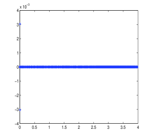
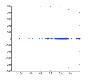
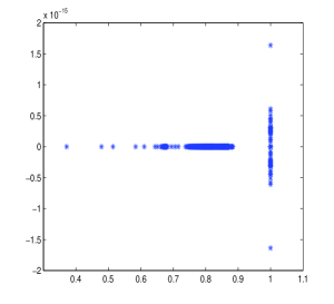
Figure 1: Eigenvalues distribution of the saddle point matrix $\mathcal{A}$ (left) and the preconditioned matrix, $\mathcal{P}_{MGSS}^{-1}\mathcal{A}$ where $\alpha=\beta=0.001$ (middle) and $\mathcal{P}_{RMGSS}^{-1}\mathcal{A}$ where $\beta=0.001$ (right) with $m=32$.

References

• [1] O. Axelsson and V.A. Barker, Finite Element Solution of Boundary Value Problems, Academic Press, Orlando, FL, 1984.
• [2] Z. Z. Bai, Optimal parameters in the HSS-like methods for saddle-point problems, Numer. Linear Algebra Appl. 16 (2009) 447-479.
• [3] Z. Z. Bai and G. H. Golub, Accelerated Hermitian and skew-Hermitian splitting methods for saddle-point problems, IMA J. Numer. Anal. 27 (2007) 1-23.
• [4] Z. Z. Bai, G. H. Golub and M. K. Ng, Hermitian and skew-Hermitian splitting methods for non-Hermitian positive definite linear systems, SIAM J. Matrix Anal. Appl. 24 (2003) 603-626.
• [5] Z. Z. Bai, G. H. Golub and J. Y. Pan, Preconditioned Hermitian and skew-Hermitian splitting methods for non-Hermitian positive semidefinite linear systems, Numer. Math. 98 (2004) 1-32.
• [6] Z. Z. Bai, B. Parlett and Z. Q. Wang, On generalized successive overrelaxation methods for augmented linear systems, Numer. Math. 102 (2005) 1-38.
• [7] Z. Z. Bai and Z. Q. Wang, On parameterized inexact Uzawa methods for generalized saddle point problems, Linear Algebra Appl. 428 (2008) 2900-2932.
• [8] Z. Z. Bai, J. F. Yin and Y. F. Su, A shift-splitting preconditioner for non-Hermitian positive definite matrics, J. Comput. Math. 24 (2006) 539-552.
• [9] M. Benzi and G.H. Golub, A preconditioner for generalized saddle point problems, SIAM J. Matrix Anal. Appl. 26 (2004) 20-41.
• [10] M. Benzi, G.H. Golub and J. Liesen, Numerical solution of saddle point problems, Acta Numer. 14 (2005) 1-137.
• [11] M. Benzi and X.P. Guo, A dimensional split preconditioner for Stokes and linearized Navier-Stokes equations, Appl. Numer. Math. 61 (2011) 66-76.
• [12] M. Benzi, M. K. Ng, Q. Niu and Z. Wang. A relaxed dimensional fractorization preconditioner for the incompressible Navier-Stokes equations, J. Comput. Phys. 230 (2011) 6185-6202.
• [13] J. H. Bramble, J. E. Pasciak, and A. T. Vassilev, Analysis of the inexact Uzawa algorithm for saddle point problems, SIAM J. Numer. Anal. 34 (1997) 1072-1092.
• [14] F. Brezzi and M. Fortin, Mixed and Hybrid Finite Element Methods, Springer, New York, 1991.
• [15] Y. Cao, J. Du and Q. Niu, Shift-splitting preconditioners for saddle point problems, J. Comput. Appl. Math. 272 (2014) 239-250.
• [16] Y. Cao, M. Q. Jiang and Y. L. Zheng, A splitting preconditioner for saddle point problems, Numer. Linear Algebra Appl. 18 (2011) 875-895.
• [17] C. Chen and C. Ma, A generalized shift-splitting preconditioner for saddle point problems, Appl. Math. Lett. 43 (2015) 49-55.
• [18] F. Ding, P. X. Liu and J. Ding, Iterative solutions of the generalized Sylvester matrix equations by using the hierarchical identification principle, Appl. Math. Comput. 197 (2008) 41-50.
• [19] F. Ding and T. Chen, Gradient based iterative algorithms for solving a class of matrix equations, IEEE Trans. Automat. Control. 50(2005) 1216-1221.
• [20] F. Ding and T. Chen, On iterative solutions of general coupled matrix equations, SIAM J. Control Optim. 44(2006) 2269-2284.
• [21] F. Ding and H. Zhang, Gradient-based iterative algorithm for a class of the coupled matrix equations related to control systems, IET Control Theory Appl. 8(2014) 1588-1595.
• [22] H. Elman, Multigrid and Krylov subspace methods for the discrete Stokes equations, Internat. J. Numer. Methods Fluids. 22 (1996) 755-770.
• [23] H. C. Elman and G. H. Golub, Inexact and preconditioned Uzawa algorithms for saddle point problems, SIAM J. Numer. Anal. 31 (1994) 1645-1661.
• [24] H.C. Elman, A. Ramage, D.J. Silvester, IFISS: A Matlab toolbox for modelling incompressible flow, ACM Trans. Math. Software. 33 (2007), Article 14.
• [25] H. C. Elman, D. J. Silvester and A.J. Wathen, Finite Elements and Fast Iterative Solvers, Oxford University Press, Oxford, 2003.
• [26] A. Klawonn, Block-triangular preconditioners for saddle-point problems with a penalty term, SIAM J. Sci. Comput. 19 (1998) 172-184.
• [27] Y. Saad, Iterative Methods for Sparse Linear Systems, SIAM, Philadelphia, 2003.
• [28] D. Silvester and A. Wathen, Fast iterative solution of stabilized Stokes systems, Part II: Using general block preconditioners, SIAM J. Numer. Anal. 31 (1994) 1352-1367.
• [29] S.-L. Wu, T.-Z. Huang and C.-X. Li, Generalized block triangular preconditioner for symmetric saddle point problems, Computing. 84 (2009) 183-208.
• [30] S.-L. Wu, T.-Z. Huang and C.-X. Li, Modified block preconditioners for the discretized time-harmonic Maxwell equations in mixed form, J. Comput. Appl. Math. 237 (2013) 419-431.
• [31] S.-L. Wu, L. Bergamaschi and C.-X. Li, A note on eigenvalue distribution of constraint-preconditioned symmetric saddle point matrices, Numer. Linear Algebra Appl. 21 (2014) 171-174.
• [32] S.-L. Wu and C.-X. Li, Eigenvalue estimates of an indefinite block triangular preconditioner for saddle point problem, J. Comput. Appl. Math. 260 (2014) 349-355.