Efficient Algorithms for CUR and Interpolative Matrix Decompositions

Abstract

The manuscript describes efficient algorithms for the computation of the CUR and ID decompositions. The methods used are based on simple modifications to the classical truncated pivoted QR decomposition, which means that highly optimized library codes can be utilized for implementation. For certain applications, further acceleration can be attained by incorporating techniques based on randomized projections. Numerical experiments demonstrate advantageous performance compared to existing techniques for computing CUR factorizations.

1 Introduction

In many applications, it is useful to approximate a matrix $\bm{\mathsf{A}}\in\mathbb{C}^{m\times n}$ by a factorization of rank $k<\min(m,n)$. When the singular values of $\bm{\mathsf{A}}$ decay sufficiently fast so that an accurate approximation can be obtained for a rank $k$ that is substantially smaller than either $m$ or $n$, great savings can be obtained both in terms of storage requirements, and in terms of speed of any computations involving $\bm{\mathsf{A}}$. A low rank approximation that is in many ways optimal is the truncated singular value decomposition (SVD) of rank $k$, which approximates $\bm{\mathsf{A}}$ via the product

$$\begin{array}[]{ccccc}\bm{\mathsf{A}}&\approx&\bm{\mathsf{U}}_{k}&\bm{\mathsf{\Sigma}}_{k}&\bm{\mathsf{V}}^{*}_{k},\\ m\times n&&m\times k&k\times k&k\times n\end{array}$$ (1.1)

where the columns of the orthonormal matrices $\bm{\mathsf{U}}_{k}$ and $\bm{\mathsf{V}}_{k}$ are the left and right singular vectors of $\bm{\mathsf{A}}$, and where $\bm{\mathsf{\Sigma}}_{k}$ is a diagonal matrix holding the singular values of $\bm{\mathsf{A}}$. However, a disadvantage of the low rank SVD is its storage requirements. Even if $\bm{\mathsf{A}}$ is a sparse matrix, $\bm{\mathsf{U}}_{k}$ and $\bm{\mathsf{V}}_{k}$ are usually dense. This means that if $\bm{\mathsf{A}}$ is large and very sparse, compression via the SVD is only efficient when the rank $k$ is much smaller than $\min(m,n)$.

As an alternative to the SVD, the so called CUR-factorization [8, 19, 13] has recently received much attention [15, 21]. The CUR-factorization approximates an $m\times n$ matrix $\bm{\mathsf{A}}$ as a product

$$\begin{array}[]{ccccc}\bm{\mathsf{A}}&\approx&\bm{\mathsf{C}}&\bm{\mathsf{U}}&\bm{\mathsf{R}},\\ m\times n&&m\times k&k\times k&k\times n\end{array}$$ (1.2)

where $\bm{\mathsf{C}}$ contains a subset of the columns of $\bm{\mathsf{A}}$ and $\bm{\mathsf{R}}$ contains a subset of the rows of $\bm{\mathsf{A}}$. The key advantage of the CUR is that the factors $\bm{\mathsf{C}}$ and $\bm{\mathsf{R}}$ (which are typically much larger than $\bm{\mathsf{U}}$) inherit properties such as sparsity or non-negativity from $\bm{\mathsf{A}}$. Also, the index sets that point out which columns and rows of $\bm{\mathsf{A}}$ to include in $\bm{\mathsf{C}}$ and $\bm{\mathsf{R}}$ often assist in data interpretation. Numerous algorithms for computing the CUR factorization have been proposed (see e.g. [5, 21]), with some of the most recent and popular approaches relying on a method known as leverage scores [5, 13], a notion originating from statistics [11].

A third factorization which is closely related to the CUR is the so called interpolative decomposition (ID), which decomposes $\bm{\mathsf{A}}$ as

$$\begin{array}[]{ccccc}\bm{\mathsf{A}}&\approx&\bm{\mathsf{C}}&\bm{\mathsf{V}}^{*},\\ m\times n&&m\times k&k\times n\end{array}$$ (1.3)

where again $\bm{\mathsf{C}}$ consists of $k$ columns of $\bm{\mathsf{A}}$. The matrix $\bm{\mathsf{V}}$ contains a $k\times k$ identity matrix as a submatrix and can be constructed so that $\max_{i,j}|\bm{\mathsf{V}}(i,j)|\leq 1$, making $\bm{\mathsf{V}}$ fairly well-conditioned. Of course, one could equally well express $\bm{\mathsf{A}}$ as

$$\begin{array}[]{ccccc}\bm{\mathsf{A}}&\approx&\bm{\mathsf{W}}&\bm{\mathsf{R}},\\ m\times n&&m\times k&k\times n\end{array}$$ (1.4)

where $\bm{\mathsf{R}}$ holds $k$ rows of $\bm{\mathsf{A}}$, and the properties of $\bm{\mathsf{W}}$ are analogous to those of $\bm{\mathsf{V}}$. A third variation of this idea is the two-sided interpolative decomposition (tsID), which decomposes $\bm{\mathsf{A}}$ as the product

$$\begin{array}[]{ccccc}\bm{\mathsf{A}}&\approx&\bm{\mathsf{W}}&\bm{\mathsf{A}}_{\rm skel}&\bm{\mathsf{V}}^{*},\\ m\times n&&m\times k&k\times k&k\times n\end{array}$$ (1.5)

where $\bm{\mathsf{A}}_{\rm skel}$ consists of a $k\times k$ submatrix of $\bm{\mathsf{A}}$. The two sided ID allows for data interpretation in a manner entirely analogous to the CUR, but has an advantage over the CUR in that it is inherently better conditioned, cf. Remark 2.3. On the other hand, the factors $\bm{\mathsf{W}}$ and $\bm{\mathsf{V}}$ do not inherit properties such as sparsity or non-negativity. This makes the two-sided ID only marginally better than the SVD in terms of storage requirements for sparse matrices.

In this manuscript, we describe a set of efficient algorithms for computing approximate ID and CUR factorizations. The algorithms are obtained via slight variations on the classical “rank-revealing QR” factorizations [4] and are easy to implement—the most expensive parts of the computation can be executed using highly optimized standard libraries such as, e.g., LAPACK [1]. We also demonstrate how the computations can be accelerated by using randomized algorithms [10]. For instance, randomization allows us to improve the asymptotic complexity of computing the CUR decomposition from $O(mnk)$ to $O(mn\,log(k)+(m+n)k^{2})$. Section 6 illustrates via several numerical examples that the techniques described here for computing the CUR factorization compare favorably in terms of both speed and accuracy with recently proposed CUR implementations. All the ID and CUR factorization algorithms discussed in this article are efficiently implemented as part of the open source RSVDPACK package [20].

2 Preliminaries

In this section we review some existing matrix decompositions, notably the pivoted QR , ID , and CUR  decompositions [10]. We follow the notation of [7] (the so called “Matlab style notation”): given any matrix $\bm{\mathsf{A}}$ and (ordered) subindex sets $I$ and $J$, $\bm{\mathsf{A}}(I,J)$ denotes the submatrix of $\bm{\mathsf{A}}$ obtained by extracting the rows and columns of $\bm{\mathsf{A}}$ indexed by $I$ and $J$, respectively; and $\bm{\mathsf{A}}(:,J)$ denotes the submatrix of $\bm{\mathsf{A}}$ obtained by extracting the columns of $\bm{\mathsf{A}}$ indexed by $J$. For any positive integer $k$, $1:k$ denotes the ordered index set $(1,\ldots,k)$. We take $\|\cdot\|$ to be the spectral or operator norm (largest singular value) and $\|\cdot\|_{F}$ the Frobenius norm: $\|x\|_{F}=\left(\displaystyle\sum_{k=1}^{n}|x_{k}|^{2}\right)^{\frac{1}{2}}$.

2.1 The singular value decomposition (SVD)

The SVD was introduced briefly in the introduction. Here we define it again, with some more detail added. Let $\bm{\mathsf{A}}$ denote an $m\times n$ matrix, and set $r=\min(m,n)$. Then $\bm{\mathsf{A}}$ admits a factorization

$$\begin{array}[]{ccccccccccccccccccccc}\bm{\mathsf{A}}&=&\bm{\mathsf{U}}&\bm{\mathsf{\Sigma}}&\bm{\mathsf{V}}^{*},\\ m\times n&&m\times r&r\times r&r\times n\end{array}$$ (2.1)

where the matrices $\bm{\mathsf{U}}$ and $\bm{\mathsf{V}}$ are orthonormal, and $\bm{\mathsf{\Sigma}}$ is diagonal. We let $\{\bm{\mathsf{u}}_{i}\}_{i=1}^{r}$ and $\{\bm{\mathsf{v}}_{i}\}_{i=1}^{r}$ denote the columns of $\bm{\mathsf{U}}$ and $\bm{\mathsf{V}}$, respectively. These vectors are the left and right singular vectors of $\bm{\mathsf{A}}$. As in the introduction, the diagonal elements $\{\sigma_{j}\}_{j=1}^{r}$ of $\bm{\mathsf{\Sigma}}$ are the singular values of $\bm{\mathsf{A}}$. We order these so that $\sigma_{1}\geq\sigma_{2}\geq\cdots\geq\sigma_{r}\geq 0$. We let $\bm{\mathsf{A}}_{k}$ denote the truncation of the SVD to its first $k$ terms, $\bm{\mathsf{A}}_{k}=\sum_{i=1}^{k}\sigma_{i}\,\bm{\mathsf{u}}_{i}\,\bm{\mathsf{v}}_{j}^{*}$. It is easily verified that

$$\|\bm{\mathsf{A}}-\bm{\mathsf{A}}_{k}\|=\sigma_{k+1},\qquad\mbox{and that}\qquad\|\bm{\mathsf{A}}-\bm{\mathsf{A}}_{k}\|_{F}=\left(\sum_{j=k+1}^{\min(m,n)}\sigma_{j}^{2}\right)^{1/2}.$$ (2.2)

Moreover, the Eckart-Young theorem [6] states that these errors are the smallest possible errors that can be incurred when approximating $\bm{\mathsf{A}}$ by a matrix of rank $k$.

2.2 Pivoted QR factorizations

Let $\bm{\mathsf{A}}$ be an $m\times n$ matrix with real or complex entries, and set $r=\min(m,n)$. The (compact) QR-factorization of $\bm{\mathsf{A}}$ then takes the form

$$\begin{array}[]{ccccccc}\bm{\mathsf{A}}&\bm{\mathsf{P}}&=&\bm{\mathsf{Q}}&\bm{\mathsf{S}},\\ m\times n&n\times n&&m\times r&r\times n\end{array}$$ (2.3)

where $\bm{\mathsf{P}}$ is a permutation matrix, $\bm{\mathsf{Q}}$ has orthonormal columns, and $\bm{\mathsf{S}}$ is upper triangular (the matrix we call “$\bm{\mathsf{S}}$” is customarily labeled “$\bm{\mathsf{R}}$”, but we use that letter for one of the factors in the CUR-decomposition). The permutation matrix $\bm{\mathsf{P}}$ can more efficiently be represented via a vector $J\in\mathbb{Z}_{+}^{n}$ of indices such that $\bm{\mathsf{P}}=\bm{\mathsf{I}}(:,J)$ where $\bm{\mathsf{I}}$ is the $n\times n$ identity matrix. The factorization (2.3) can then be written

$$\begin{array}[]{ccccccc}\bm{\mathsf{A}}(:,J)&=&\bm{\mathsf{Q}}&\bm{\mathsf{S}}.\\ m\times n&&m\times r&r\times n\end{array}$$ (2.4)

The QR-factorization is often computed via column pivoting combined with either the Gram-Schmidt process, Householder reflectors [7], or Givens rotations [4]. The resulting factor $\bm{\mathsf{S}}$ then satisfies various decay conditions [7], such as:

$$\bm{\mathsf{S}}(j,j)\geq\|\bm{\mathsf{S}}(j:m,\ell)\|_{2}\qquad\mbox{for all}\ j<\ell.$$

The QR-factorization (2.4) expresses $\bm{\mathsf{A}}$ as a sum of $r$ rank-one matrices

$$\bm{\mathsf{A}}(:,J)\approx\sum_{j=1}^{r}\bm{\mathsf{Q}}(:,j)\,\bm{\mathsf{S}}(j,:).$$

The QR-factorization is often built incrementally via a greedy algorithm such as column pivoted Gram-Schmidt. This opens up the possibility of stopping after the first $k$ terms have been computed and settling for a “partial QR-factorization of $\bm{\mathsf{A}}$”. We can express the error term by splitting the factors in (2.4) as follows:

$$\bm{\mathsf{A}}(:,J)\quad=\quad\hbox{}\vbox{\kern 0.86108pt\hbox{$\kern 0.0pt\kern 2.5pt\kern-5.0pt\left[\kern 0.0pt\kern-2.5pt\kern-5.55557pt\vbox{\kern-0.86108pt\vbox{\vbox{ \halign{\kern\arraycolsep\hfil\@arstrut$\kbcolstyle#$\hfil\kern\arraycolsep& \kern\arraycolsep\hfil$\@kbrowstyle#$\ifkbalignright\relax\else\hfil\fi\kern\arraycolsep&& \kern\arraycolsep\hfil$\@kbrowstyle#$\ifkbalignright\relax\else\hfil\fi\kern\arraycolsep\cr 5.0pt\hfil\@arstrut$\scriptstyle$\hfil\kern 5.0pt&5.0pt\hfil$\scriptstyle k$\hfil\kern 5.0pt&5.0pt\hfil$\scriptstyle r-k\\m$\hfil\kern 5.0pt&5.0pt\hfil$\scriptstyle\bm{\mathsf{Q}}_{1}$\hfil\kern 5.0pt&5.0pt\hfil$\scriptstyle\bm{\mathsf{Q}}_{2}$\hfil\kern 5.0pt\crcr}}}}\right]$}}\times\hbox{}\vbox{\kern 0.86108pt\hbox{$\kern 0.0pt\kern 2.5pt\kern-5.0pt\left[\kern 0.0pt\kern-2.5pt\kern-5.55557pt\vbox{\kern-0.86108pt\vbox{\vbox{ \halign{\kern\arraycolsep\hfil\@arstrut$\kbcolstyle#$\hfil\kern\arraycolsep& \kern\arraycolsep\hfil$\@kbrowstyle#$\ifkbalignright\relax\else\hfil\fi\kern\arraycolsep&& \kern\arraycolsep\hfil$\@kbrowstyle#$\ifkbalignright\relax\else\hfil\fi\kern\arraycolsep\cr 5.0pt\hfil\@arstrut$\scriptstyle$\hfil\kern 5.0pt&5.0pt\hfil$\scriptstyle n\\k$\hfil\kern 5.0pt&5.0pt\hfil$\scriptstyle\bm{\mathsf{S}}_{1}\\r-k$\hfil\kern 5.0pt&5.0pt\hfil$\scriptstyle\bm{\mathsf{S}}_{2}$\hfil\kern 5.0pt\crcr}}}}\right]$}}\ =\ \bm{\mathsf{Q}}_{1}\bm{\mathsf{S}}_{1}+\bm{\mathsf{Q}}_{2}\bm{\mathsf{S}}_{2}.$$ (2.5)

Observe that since the SVD is optimal, it is always the case that

$$\sigma_{k+1}(\bm{\mathsf{A}})\leq\|\bm{\mathsf{Q}}_{2}\,\bm{\mathsf{S}}_{2}\|=\|\bm{\mathsf{S}}_{2}\|.$$

We say that a factorization is a “rank-revealing QR-factorization (RRQR)” if the ratio $\frac{\|\bm{\mathsf{S}}_{2}\|}{\sigma_{k+1}(\bm{\mathsf{A}})}$ is guaranteed to be bounded [9]. (Some authors require additionally that $\sigma_{j}(\bm{\mathsf{S}}_{1})\approx\sigma_{j}(\bm{\mathsf{A}})$ for $1\leq j\leq k$). Classical column pivoted Gram-Schmidt typically results in an RRQR, but there are counter-examples. More sophisticated versions such as [9] provably compute an RRQR, but are substantially harder to code, and the gain compared to standard methods is typically modest.

2.3 Low rank interpolative decomposition

An approximate rank $k$ interpolative decomposition (ID) of a matrix $\bm{\mathsf{A}}\in\mathbb{C}^{m\times n}$ is the approximate factorization:

$$\begin{array}[]{cccc}\bm{\mathsf{A}}&\approx&\bm{\mathsf{C}}&\bm{\mathsf{V}}^{*},\\ m\times n&&m\times k&k\times n\end{array}$$ (2.6)

where the partial column skeleton $\bm{\mathsf{C}}\in\mathbb{C}^{m\times k}$ is given by a subset of the columns of $\bm{\mathsf{A}}$ and $\bm{\mathsf{V}}$ is well-conditioned in a sense that we will make precise shortly. The interpolative decomposition approximates $\bm{\mathsf{A}}$ using only some of its columns, and one of the advantages of doing so is that the more compact description of the range of $\bm{\mathsf{A}}$ given by its skeleton preserves some of the properties of the original matrix $\bm{\mathsf{A}}$ such as sparsity and non-negativity. In this section we show one way of obtaining a low rank interpolative decomposition, via the truncated QR with column pivoting.

From (2.5), we see that as long as $\|\bm{\mathsf{S}}_{2}\|_{2}$ is small, we can approximate $\bm{\mathsf{A}}(:,J)$ by $\bm{\mathsf{Q}}_{1}\bm{\mathsf{S}}_{1}$. We show that the approximation term $\bm{\mathsf{Q}}_{1}\bm{\mathsf{S}}_{1}$ provides a rank $k$ ID to the matrix $\bm{\mathsf{A}}$. In fact, the approximation term $\bm{\mathsf{Q}}_{1}\bm{\mathsf{S}}_{1}$ is the image of a skeleton of $\bm{\mathsf{A}}$, i.e., the range of $\bm{\mathsf{Q}}_{1}\bm{\mathsf{S}}_{1}$ is contained in the span of $k$ columns of $\bm{\mathsf{A}}$. Splitting the columns of $\bm{\mathsf{S}}_{1}$ and $\bm{\mathsf{S}}_{2}$ as follows:

$$\bm{\mathsf{S}}_{1}=\ \hbox{}\vbox{\kern 0.86108pt\hbox{$\kern 0.0pt\kern 2.5pt\kern-5.0pt\left[\kern 0.0pt\kern-2.5pt\kern-5.55557pt\vbox{\kern-0.86108pt\vbox{\vbox{ \halign{\kern\arraycolsep\hfil\@arstrut$\kbcolstyle#$\hfil\kern\arraycolsep& \kern\arraycolsep\hfil$\@kbrowstyle#$\ifkbalignright\relax\else\hfil\fi\kern\arraycolsep&& \kern\arraycolsep\hfil$\@kbrowstyle#$\ifkbalignright\relax\else\hfil\fi\kern\arraycolsep\cr 5.0pt\hfil\@arstrut$\scriptstyle$\hfil\kern 5.0pt&5.0pt\hfil$\scriptstyle k$\hfil\kern 5.0pt&5.0pt\hfil$\scriptstyle n-k\\k$\hfil\kern 5.0pt&5.0pt\hfil$\scriptstyle\bm{\mathsf{S}}_{11}$\hfil\kern 5.0pt&5.0pt\hfil$\scriptstyle\bm{\mathsf{S}}_{12}$\hfil\kern 5.0pt\crcr}}}}\right]$}}\quad\mbox{and}\quad\bm{\mathsf{S}}_{2}=\ \hbox{}\vbox{\kern 0.86108pt\hbox{$\kern 0.0pt\kern 2.5pt\kern-5.0pt\left[\kern 0.0pt\kern-2.5pt\kern-5.55557pt\vbox{\kern-0.86108pt\vbox{\vbox{ \halign{\kern\arraycolsep\hfil\@arstrut$\kbcolstyle#$\hfil\kern\arraycolsep& \kern\arraycolsep\hfil$\@kbrowstyle#$\ifkbalignright\relax\else\hfil\fi\kern\arraycolsep&& \kern\arraycolsep\hfil$\@kbrowstyle#$\ifkbalignright\relax\else\hfil\fi\kern\arraycolsep\cr 5.0pt\hfil\@arstrut$\scriptstyle$\hfil\kern 5.0pt&5.0pt\hfil$\scriptstyle k$\hfil\kern 5.0pt&5.0pt\hfil$\scriptstyle n-k\\r-k$\hfil\kern 5.0pt&5.0pt\hfil$\scriptstyle\bm{\mathsf{0}}$\hfil\kern 5.0pt&5.0pt\hfil$\scriptstyle\bm{\mathsf{S}}_{22}$\hfil\kern 5.0pt\crcr}}}}\right]$}},\quad(\text{i.e., }\ \ \bm{\mathsf{S}}=\hbox{}\vbox{\kern 0.86108pt\hbox{$\kern 0.0pt\kern 2.5pt\kern-5.0pt\left[\kern 0.0pt\kern-2.5pt\kern-5.55557pt\vbox{\kern-0.86108pt\vbox{\vbox{ \halign{\kern\arraycolsep\hfil\@arstrut$\kbcolstyle#$\hfil\kern\arraycolsep& \kern\arraycolsep\hfil$\@kbrowstyle#$\ifkbalignright\relax\else\hfil\fi\kern\arraycolsep&& \kern\arraycolsep\hfil$\@kbrowstyle#$\ifkbalignright\relax\else\hfil\fi\kern\arraycolsep\cr 5.0pt\hfil\@arstrut$\scriptstyle$\hfil\kern 5.0pt&5.0pt\hfil$\scriptstyle k$\hfil\kern 5.0pt&5.0pt\hfil$\scriptstyle n-k\\k$\hfil\kern 5.0pt&5.0pt\hfil$\scriptstyle\bm{\mathsf{S}}_{11}$\hfil\kern 5.0pt&5.0pt\hfil$\scriptstyle\bm{\mathsf{S}}_{12}\\r-k$\hfil\kern 5.0pt&5.0pt\hfil$\scriptstyle\bm{\mathsf{0}}$\hfil\kern 5.0pt&5.0pt\hfil$\scriptstyle\bm{\mathsf{S}}_{22}$\hfil\kern 5.0pt\crcr}}}}\right]$}},\ )$$ (2.7)

it is immediate that

$$\bm{\mathsf{A}}(:,J)\ =\ \bm{\mathsf{Q}}_{1}\begin{bmatrix}\bm{\mathsf{S}}_{11}&\bm{\mathsf{S}}_{12}\end{bmatrix}+\bm{\mathsf{Q}}_{2}\begin{bmatrix}0&\bm{\mathsf{S}}_{22}\end{bmatrix}\ =\ \hbox{}\vbox{\kern 0.86108pt\hbox{$\kern 0.0pt\kern 2.5pt\kern-5.0pt\left[\kern 0.0pt\kern-2.5pt\kern-5.55557pt\vbox{\kern-0.86108pt\vbox{\vbox{ \halign{\kern\arraycolsep\hfil\@arstrut$\kbcolstyle#$\hfil\kern\arraycolsep& \kern\arraycolsep\hfil$\@kbrowstyle#$\ifkbalignright\relax\else\hfil\fi\kern\arraycolsep&& \kern\arraycolsep\hfil$\@kbrowstyle#$\ifkbalignright\relax\else\hfil\fi\kern\arraycolsep\cr 5.0pt\hfil\@arstrut$\scriptstyle$\hfil\kern 5.0pt&5.0pt\hfil$\scriptstyle k$\hfil\kern 5.0pt&5.0pt\hfil$\scriptstyle n-k\\m$\hfil\kern 5.0pt&5.0pt\hfil$\scriptstyle\bm{\mathsf{Q}}_{1}\bm{\mathsf{S}}_{11}$\hfil\kern 5.0pt&5.0pt\hfil$\scriptstyle\bm{\mathsf{Q}}_{1}\bm{\mathsf{S}}_{12}+\bm{\mathsf{Q}}_{2}\bm{\mathsf{S}}_{22}$\hfil\kern 5.0pt\crcr}}}}\right]$}}.$$

In other words, we see that the matrix $\bm{\mathsf{Q}}_{1}\bm{\mathsf{S}}_{11}$ equals the first $k$ columns of $\bm{\mathsf{A}}(:,J)$. We now define the factor $\bm{\mathsf{C}}$ in (2.6) via

$$\bm{\mathsf{C}}\ :=\ \bm{\mathsf{A}}(:,J(1:k))\ =\ \bm{\mathsf{Q}}_{1}\bm{\mathsf{S}}_{11}.$$

Then the dominant term $\bm{\mathsf{Q}}_{1}\bm{\mathsf{S}}_{1}$ in (2.5) can be written

$$\bm{\mathsf{Q}}_{1}\bm{\mathsf{S}}_{1}\ =\ \begin{bmatrix}\bm{\mathsf{Q}}_{1}\bm{\mathsf{S}}_{11}&\bm{\mathsf{Q}}_{1}\bm{\mathsf{S}}_{12}\end{bmatrix}\ =\ \bm{\mathsf{Q}}_{1}\bm{\mathsf{S}}_{11}\,[\bm{\mathsf{I}}_{k}\quad\bm{\mathsf{T}}_{l}].\ =\ \bm{\mathsf{C}}\,[\bm{\mathsf{I}}_{k}\quad\bm{\mathsf{T}}_{l}],$$

where $\bm{\mathsf{T}}_{l}$ is a solution to the matrix equation

$$\bm{\mathsf{S}}_{11}\bm{\mathsf{T}}_{l}=\bm{\mathsf{S}}_{12}.$$ (2.8)

The equation (2.8) obviously has a solution whenever $\bm{\mathsf{S}}_{11}$ is non-singular. If $\bm{\mathsf{S}}_{11}$ is singular, then one can show that $\bm{\mathsf{A}}$ must necessarily have rank $k^{\prime}$ less than $k$, and the bottom $k-k^{\prime}$ rows in (2.8) consist of all zeros, so there exists a solution in this case as well. We now recover the factorization (2.6) upon setting

$${\bm{\mathsf{V}}}^{*}=\begin{bmatrix}\bm{\mathsf{I}}_{k}&\bm{\mathsf{T}}_{l}\end{bmatrix}\bm{\mathsf{P}}^{*}.$$ (2.9)

The approximation error of the ID obtained via truncated QR with pivoting is the same as that of the truncated QR:

$$\bm{\mathsf{A}}-\bm{\mathsf{C}}\bm{\mathsf{V}}^{*}=\bm{\mathsf{Q}}_{2}\bm{\mathsf{S}}_{22}$$ (2.10)

Remark 2.1

This section describes a technique for converting a QR decomposition of $\bm{\mathsf{A}}$ into the interpolative decomposition (1.3). By applying an analogous procedure to the adjoint $\bm{\mathsf{A}}^{*}$ of $\bm{\mathsf{A}}$, we obtain the sibling factorization (1.4) that uses a sub-selection of rows of $\bm{\mathsf{A}}$ to span the row space. In other words, to find the column skeleton, we perform Gram-Schmidt on the columns on $\bm{\mathsf{A}}$, and in order to find the row skeleton, we perform Gram-Schmidt to the rows of $\bm{\mathsf{A}}$.

2.4 Two sided interpolative decomposition

A two sided ID approximation for matrices, is constructed via two successive one sided IDs. Assume that we have performed the one sided decomposition to obtain (2.9). Then perform an ID of the adjoint of $\bm{\mathsf{C}}$ to determine a matrix $\bm{\mathsf{W}}$ and an index vector $I$ such that

$$\begin{array}[]{cccccccccccccccc}\bm{\mathsf{C}}^{*}&=&\bm{\mathsf{C}}(I(1:k),:)^{*}&\bm{\mathsf{W}}^{*}.\\ k\times m&&k\times k&k\times m\end{array}$$ (2.11)

In other words, the index vector $I$ is obtained by performing a pivoted Gram-Schmidt process on the rows of $\bm{\mathsf{C}}$. Observe that the factorization (2.11) is exact since it is a full (as opposed to partial) QR factorization. We next insert (2.11) into (2.6), using that $\bm{\mathsf{C}}(I(1:k),:)=\bm{\mathsf{A}}(I(1:k),J(1:k))$, and obtain

$$\bm{\mathsf{A}}\ \approx\ \bm{\mathsf{C}}\bm{\mathsf{V}}^{*}=\bm{\mathsf{W}}\bm{\mathsf{A}}(I(1:k),J(1:k))\bm{\mathsf{V}}^{*}.$$ (2.12)

We observe that the conversion of the single-sided ID (2.9) into the two-sided ID (2.12) is exact in the sense that no additional approximation error is incurred:

$$\bm{\mathsf{A}}-\bm{\mathsf{C}}\,\bm{\mathsf{V}}^{*}=\bm{\mathsf{A}}-\bm{\mathsf{W}}\,\bm{\mathsf{A}}(I(1:k),J(1:k))\,\bm{\mathsf{V}}^{*}=\bm{\mathsf{Q}}_{2}\bm{\mathsf{S}}_{2}.$$

Remark 2.2

The index vector $I$ and the basis matrix $\bm{\mathsf{W}}$ computed using the approach described in this section form an approximate row-ID for $\bm{\mathsf{A}}$ in the sense that $\bm{\mathsf{A}}\approx\bm{\mathsf{W}}\,\bm{\mathsf{A}}(I,:)$. However, the resulting error tends to be slightly higher than the error incurred if Gram-Schmidt is performed directly on the rows of $\bm{\mathsf{A}}$ (rather than on the rows of $\bm{\mathsf{C}}$), cf. Lemma 3.2.

2.5 The CUR Decomposition

A rank $k$ CUR factorization of a matrix $\bm{\mathsf{A}}\in\mathbb{C}^{m\times n}$ is given by

$$\begin{array}[]{ccccccc}\bm{\mathsf{A}}&\approx&\bm{\mathsf{C}}&\bm{\mathsf{U}}&\bm{\mathsf{R}},\\ m\times n&&m\times k&k\times k&k\times n\end{array}$$

where $\bm{\mathsf{C}}$ consists of $k$ columns of $\bm{\mathsf{A}}$, and $\bm{\mathsf{R}}$ consists of $k$ rows of $\bm{\mathsf{A}}$. The decomposition is typically obtained in three steps [15]. First, some scheme is used to assign a weight or the so called leverage score (of importance) to each column and row in the matrix. This is typically done either using the $\ell_{2}$ norms of the columns and rows or by using the leading singular vectors of $\bm{\mathsf{A}}$ [5]. Next, the matrices $\bm{\mathsf{C}}$ and $\bm{\mathsf{R}}$ are constructed via a randomized sampling procedure, using the leverage scores to assign a sampling probability to each column and row. Finally, the $\bm{\mathsf{U}}$ matrix is computed via:

$$\bm{\mathsf{U}}\approx\bm{\mathsf{C}}^{\dagger}\bm{\mathsf{A}}\bm{\mathsf{R}}^{\dagger},$$ (2.13)

with $\bm{\mathsf{C}}^{\dagger}$ and $\bm{\mathsf{R}}^{\dagger}$ being the pseudoinverses of $\bm{\mathsf{C}}$ and $\bm{\mathsf{R}}$.

Many techniques for computing CUR factorizations have been proposed. In particular, we mention the recent work of Sorensen and Embree [18] on the DEIM-CUR method. A number of standard CUR algorithms is implemented in the software package rCUR [2] which we use for our numerical comparisons. The methods in the rCUR package utilize eigenvectors to assign weights to columns and rows of $\bm{\mathsf{A}}$. Computing the eigenvectors exactly amounts to doing the SVD which is very expensive. However, instead of the full SVD, when a CUR of rank $k$ is required, we can utilize instead the randomized SVD algorithm [10] to compute an approximate SVD of rank $k$ at substantially lower cost.

Remark 2.3 (Conditioning of CUR)

For matrices whose singular value experience substantial decay, the accuracy of the CUR factorization can deteriorate due to effects of ill-conditioning. To simplify slightly, one would normally expect the leading $k$ singular values of $\bm{\mathsf{C}}$ and $\bm{\mathsf{R}}$ to be of roughly the same order of magnitude as the leading $k$ singular values of $\bm{\mathsf{A}}$. Since low-rank factorizations are most useful when applied to matrices whose singular values decay reasonably rapidly, we would typically expect $\bm{\mathsf{C}}$ and $\bm{\mathsf{R}}$ to be highly ill-conditioned, with condition numbers roughly on the order of $\sigma_{1}(\bm{\mathsf{A}})/\sigma_{k}(\bm{\mathsf{A}})$. Hence, in the typical case, evaluation of the formula (2.13) can be expected to result in substantial loss of accuracy due to accumulation of round-off errors. Observe that the ID does not suffer from this problem; in (1.5), the matrix $\bm{\mathsf{A}}_{\rm skel}$ tends to be ill-conditioned, but it does not need to be inverted. (The matrices $\bm{\mathsf{W}}$ and $\bm{\mathsf{V}}$ are well-conditioned.)

3 The CUR-ID algorithm

In this section, we demonstrate that the CUR decomposition can easily be constructed from the basic two-sided ID (which in turn, recall, can be built from a column pivoted QR factorization), via a procedure we call “CUR-ID”. The difference between recently popularized algorithms for CUR computation and CUR-ID is in the choice of columns and rows of $\bm{\mathsf{A}}$ for forming $\bm{\mathsf{C}}$ and $\bm{\mathsf{R}}$. In the CUR-ID algorithm, the columns and rows are chosen via the two sided ID. The idea behind the use of ID for obtaining the CUR factorization is that the matrix $\bm{\mathsf{C}}$ in the CUR factorization is immediately available from the ID  (see (2.9)), and the matrix $\bm{\mathsf{V}}\in\mathbb{C}^{n\times k}$ not only captures a rough row space description of $\bm{\mathsf{A}}$ but also is of rank at most $k$. A rank $k$ ID on $\bm{\mathsf{C}}$, being an exact factorization of $\bm{\mathsf{C}}$ which is of rank at most $k$, could hint on the relevant rows of $\bm{\mathsf{A}}$ that approximate the entire row space of $\bm{\mathsf{A}}$ itself. Specifically, similar to (2.9) where approximating $\operatorname{range}(\bm{\mathsf{A}})$ using $\bm{\mathsf{C}}$ incurs an error term $\begin{bmatrix}\bm{\mathsf{0}}&\bm{\mathsf{Q}}_{2}S_{22}\end{bmatrix}$, we can estimate the error of approximating $\operatorname{range}(\bm{\mathsf{A}}^{*})$ using $\bm{\mathsf{A}}(I(1:k),:)$; see Lemma 3.2 below.

The CUR-ID algorithm is based on the two sided ID factorization, and as a starting point, we assume the factorization (2.12) has been computed using the procedures described in Section 2. In other words, we assume that the index vectors $I$ and $J$, and the basis matrices $\bm{\mathsf{V}}$ and $\bm{\mathsf{W}}$, are all available. We then define

$$\bm{\mathsf{C}}\ =\ \bm{\mathsf{A}}(:,J(1:k))\quad\text{and}\quad\bm{\mathsf{R}}=\bm{\mathsf{A}}(I(1:k),:).$$ (3.1)

Consequently, $\bm{\mathsf{C}}$ and $\bm{\mathsf{R}}$ are respectively subsets of columns and of rows of $\bm{\mathsf{A}}$, with $J$ and $I$ determined by the pivoted QR factorizations. Next we construct a $k\times k$ matrix $\bm{\mathsf{U}}$ such that $\bm{\mathsf{A}}\approx\bm{\mathsf{C}}\bm{\mathsf{U}}\bm{\mathsf{R}}$. We know that

$$\bm{\mathsf{A}}\approx\bm{\mathsf{C}}\,\bm{\mathsf{V}}^{*},$$ (3.2)

and we seek a factor $\bm{\mathsf{U}}$ such that

$$\bm{\mathsf{A}}\approx\bm{\mathsf{C}}\,\bm{\mathsf{U}}\,\bm{\mathsf{R}}.$$ (3.3)

By inspecting (3.2) and (3.3), we find that we would achieve our objective if we could determine a matrix $\bm{\mathsf{U}}$ such that

$$\begin{array}[]{cccccccccccccc}\bm{\mathsf{U}}&\bm{\mathsf{R}}&=&\bm{\mathsf{V}}^{*}.\\ k\times k&k\times m&&k\times m\end{array}$$ (3.4)

Unfortunately, (3.4) is an over-determined system, but at least intuitively, it seems plausible that it should have a fairly accurate solution, given that the rows of $\bm{\mathsf{R}}$ and the rows of $\bm{\mathsf{V}}^{*}$ should, by construction, span roughly the same space (namely, the space spanned by the $k$ leading right singular vectors of $\bm{\mathsf{A}}$). Solving (3.4) in the least-square sense, we arrive at our definition of $\bm{\mathsf{U}}$:

$$\bm{\mathsf{U}}:=\bm{\mathsf{V}}^{*}\bm{\mathsf{R}}^{\dagger}.$$ (3.5)

The construction of $\bm{\mathsf{C}}$, $\bm{\mathsf{U}}$, and $\bm{\mathsf{R}}$ in the previous paragraph was based on heuristics. We next demonstrate that the approximation error is comparable to the error resulting from the original QR-factorization. First, let us define $\bm{\mathsf{E}}$ and $\tilde{\bm{\mathsf{E}}}$ as the errors in the column and row IDs of $\bm{\mathsf{A}}$, respectively,

$$\bm{\mathsf{A}}= \ \bm{\mathsf{C}}\,\bm{\mathsf{V}}^{*}+\bm{\mathsf{E}},$$ (3.6)

$$\bm{\mathsf{A}}= \ \bm{\mathsf{W}}\,\bm{\mathsf{R}}+\tilde{\bm{\mathsf{E}}}.$$ (3.7)

Recall that $\bm{\mathsf{E}}$ is a quantity we can control by continuing the original QR factorization until $\|\bm{\mathsf{E}}\|$ is smaller than some given threshold. We will next prove two lemmas. The first states that the error in the CUR decomposition is bounded by $\|\bm{\mathsf{E}}\|+\|\tilde{\bm{\mathsf{E}}}\|$. The second states that $\|\tilde{\bm{\mathsf{E}}}\|$ is small whenever $\|\bm{\mathsf{E}}\|$ is small (and again, $\|\bm{\mathsf{E}}\|$ we can control).

Lemma 3.1

Let $\bm{\mathsf{A}}$ be an $m\times n$ matrix that satisfies the approximate factorizations (3.6) and (3.7). Suppose further that $\bm{\mathsf{R}}$ is full rank, and that the $k\times k$ matrix $\bm{\mathsf{U}}$ is defined by (3.5). Then

$$\|\bm{\mathsf{A}}-\bm{\mathsf{C}}\bm{\mathsf{U}}\bm{\mathsf{R}}\|\leq\|\bm{\mathsf{E}}\|+\|\tilde{\bm{\mathsf{E}}}\|.$$ (3.8)

• Using first (3.5) and then (3.6), we find

  $$\bm{\mathsf{A}}-\bm{\mathsf{C}}\bm{\mathsf{U}}\bm{\mathsf{\bm{\mathsf{R}}}}=\bm{\mathsf{A}}-\bm{\mathsf{C}}\bm{\mathsf{V}}^{*}\bm{\mathsf{\bm{\mathsf{R}}}}^{\dagger}\bm{\mathsf{\bm{\mathsf{R}}}}=\bm{\mathsf{A}}-(\bm{\mathsf{A}}-\bm{\mathsf{E}})\bm{\mathsf{R}}^{\dagger}\bm{\mathsf{R}}=\bigl{(}\bm{\mathsf{A}}-\bm{\mathsf{A}}\bm{\mathsf{R}}^{\dagger}\bm{\mathsf{R}}\bigr{)}+\bm{\mathsf{E}}\bm{\mathsf{R}}^{\dagger}\bm{\mathsf{R}}.$$ (3.9)

  To bound the term $\bm{\mathsf{A}}-\bm{\mathsf{A}}\bm{\mathsf{R}}^{\dagger}\bm{\mathsf{R}}$ we use (3.7) and the fact that $\bm{\mathsf{R}}\bm{\mathsf{R}}^{\dagger}\bm{\mathsf{R}}=\bm{\mathsf{R}}$ to achieve

  $$\bm{\mathsf{A}}-\bm{\mathsf{A}}\bm{\mathsf{R}}^{\dagger}\bm{\mathsf{R}}=\bm{\mathsf{A}}-(\bm{\mathsf{W}}\bm{\mathsf{R}}+\tilde{\bm{\mathsf{E}}})\bm{\mathsf{R}}^{\dagger}\bm{\mathsf{R}}=\bm{\mathsf{A}}-\bm{\mathsf{W}}\bm{\mathsf{R}}-\tilde{\bm{\mathsf{E}}}\bm{\mathsf{R}}^{\dagger}\bm{\mathsf{R}}=\tilde{\bm{\mathsf{E}}}-\tilde{\bm{\mathsf{E}}}\bm{\mathsf{R}}^{\dagger}\bm{\mathsf{R}}=\tilde{\bm{\mathsf{E}}}(I-\bm{\mathsf{R}}^{\dagger}\bm{\mathsf{R}}).$$ (3.10)

  Inserting (3.10) into (3.9) and taking the norms of the result, we get

  $$\|\bm{\mathsf{A}}-\bm{\mathsf{C}}\bm{\mathsf{U}}\bm{\mathsf{R}}\|=\|\tilde{\bm{\mathsf{E}}}(\bm{\mathsf{I}}-\bm{\mathsf{R}}^{\dagger}\bm{\mathsf{R}})+\bm{\mathsf{E}}\bm{\mathsf{R}}^{\dagger}\bm{\mathsf{R}}\|\leq\|\tilde{\bm{\mathsf{E}}}(\bm{\mathsf{I}}-\bm{\mathsf{R}}^{\dagger}\bm{\mathsf{R}})\|+\|\bm{\mathsf{E}}\bm{\mathsf{R}}^{\dagger}\bm{\mathsf{R}}\|\leq\|\tilde{\bm{\mathsf{E}}}\|+\|\bm{\mathsf{E}}\|,$$

  where in the last step we used that $\bm{\mathsf{R}}\bm{\mathsf{R}}^{\dagger}$ and $\bm{\mathsf{I}}-\bm{\mathsf{R}}\bm{\mathsf{R}}^{\dagger}$ are both orthonormal projections. $\Box$

Lemma 3.2

Let $\bm{\mathsf{A}}$ be an $m\times n$ matrix that admits the factorization (3.6), with error term $\bm{\mathsf{E}}$. Suppose further that $I=[I_{\rm skel},I_{\rm res}]$ and $\bm{\mathsf{T}}$ form the output of the ID of the matrix $\bm{\mathsf{C}}$, so that

$$\bm{\mathsf{C}}=\bm{\mathsf{W}}\bm{\mathsf{C}}(I_{\rm skel},:),\qquad\mbox{where}\qquad\bm{\mathsf{W}}=\bm{\mathsf{P}}\left[\begin{array}[]{c}\bm{\mathsf{I}}\\ \bm{\mathsf{T}}^{*}\end{array}\right],$$ (3.11)

and where $\bm{\mathsf{P}}$ is the permutation matrix for which $\bm{\mathsf{P}}\bm{\mathsf{A}}(I,:)=\bm{\mathsf{A}}$. Now define the matrix $\bm{\mathsf{R}}$ via

$$\bm{\mathsf{R}}=\bm{\mathsf{A}}(I_{\rm skel},:).$$ (3.12)

Observe that $\bm{\mathsf{R}}$ consists of the $k$ rows of $\bm{\mathsf{A}}$ selected in the skeletonization of $\bm{\mathsf{C}}$. Finally, set

$$\bm{\mathsf{F}}=\bigl{[}-\bm{\mathsf{T}}^{*}\ \ \bm{\mathsf{I}}\bigr{]}\bm{\mathsf{P}}^{*}.$$ (3.13)

Then the product $\bm{\mathsf{W}}\bm{\mathsf{R}}$ approximates $\bm{\mathsf{A}}$, with a residual error

$$\tilde{\bm{\mathsf{E}}}=\bm{\mathsf{A}}-\bm{\mathsf{W}}\bm{\mathsf{R}}=\bm{\mathsf{P}}\left[\begin{array}[]{c}\bm{\mathsf{0}}\\ \bm{\mathsf{F}}\bm{\mathsf{E}}\end{array}\right].$$ (3.14)

• From the definitions of $\bm{\mathsf{W}}$ in (3.11) and $\bm{\mathsf{R}}$ in (3.12) we find

  $$\bm{\mathsf{A}}-\bm{\mathsf{W}}\bm{\mathsf{R}}=\bm{\mathsf{P}}\bm{\mathsf{A}}(I,:)-\bm{\mathsf{W}}\bm{\mathsf{R}}=\bm{\mathsf{P}}\left[\begin{array}[]{c}\bm{\mathsf{A}}(I_{\rm skel},:)\\ \bm{\mathsf{A}}(I_{\rm res},:)\end{array}\right]-\bm{\mathsf{P}}\left[\begin{array}[]{c}\bm{\mathsf{I}}\\ \bm{\mathsf{T}}^{*}\end{array}\right]\bm{\mathsf{A}}(I_{\rm skel},:)\\ =\bm{\mathsf{P}}\left[\begin{array}[]{c}\bm{\mathsf{0}}\\ \bm{\mathsf{A}}(I_{\rm res},:)-\bm{\mathsf{T}}^{*}\bm{\mathsf{A}}(I_{\rm skel},:)\end{array}\right]=\bm{\mathsf{P}}\left[\begin{array}[]{c}\bm{\mathsf{0}}\\ \bm{\mathsf{F}}\bm{\mathsf{A}}\end{array}\right].$$ (3.15)

  To bound the term $\bm{\mathsf{F}}\bm{\mathsf{A}}$ in (3.15), we invoke (3.6) to obtain

  $$\bm{\mathsf{F}}\bm{\mathsf{A}}=\bm{\mathsf{F}}\bm{\mathsf{C}}\bm{\mathsf{V}}^{*}+\bm{\mathsf{F}}\bm{\mathsf{E}}=\{\mbox{Insert (\ref{eq:hannah1})}\}=\bm{\mathsf{F}}\bm{\mathsf{W}}\bm{\mathsf{C}}(I_{\rm skel},:)\bm{\mathsf{V}}^{*}+\bm{\mathsf{F}}\bm{\mathsf{E}}=\bm{\mathsf{F}}\bm{\mathsf{E}},$$ (3.16)

  since $\bm{\mathsf{F}}\bm{\mathsf{W}}=\bm{\mathsf{0}}$ due to (3.11) and (3.13). Finally, insert (3.16) into (3.15) to obtain (3.14). $\Box$

Equation (3.14) allows us to bound the norm of the error $\tilde{\bm{\mathsf{E}}}$ in (3.7). Simply observe that the definition of $\bm{\mathsf{F}}$ in (3.13) implies that for any matrix $\bm{\mathsf{X}}$ we have:

$$\bm{\mathsf{F}}\bm{\mathsf{X}}=\bigl{[}-\bm{\mathsf{T}}^{*}\ \ \bm{\mathsf{I}}\bigr{]}\bm{\mathsf{P}}^{*}\bm{\mathsf{X}}=\bigl{[}-\bm{\mathsf{T}}^{*}\ \ \bm{\mathsf{I}}\bigr{]}\left[\begin{matrix}\bm{\mathsf{X}}(I_{\rm skel},:)\\ \bm{\mathsf{X}}(I_{\rm res},:)\end{matrix}\right]=-\bm{\mathsf{T}}^{*}\bm{\mathsf{X}}(I_{\rm skel},:)+\bm{\mathsf{X}}(I_{\rm res},:),$$

so that:

$$\|\bm{\mathsf{F}}\bm{\mathsf{X}}\|=\|\bm{\mathsf{X}}(I_{\rm res},:)-\bm{\mathsf{T}}^{*}\bm{\mathsf{X}}(I_{\rm skel},:)\|\leq\|\bm{\mathsf{X}}(I_{\rm res},:)\|+\|\bm{\mathsf{T}}\|\,\|\bm{\mathsf{X}}(I_{\rm skel},:)\|\leq(1+\|\bm{\mathsf{T}}\|)\,\|\bm{\mathsf{X}}\|.$$ (3.17)

This leads us to the following Corollary to Lemma 3.2:

Corollary 3.3

Under the same assumptions as in Lemma 3.2, we have

$$\|\tilde{\bm{\mathsf{E}}}\|\leq(1+\|\bm{\mathsf{T}}\|)\,\|\bm{\mathsf{E}}\|.$$ (3.18)

Further, assuming additionally that the conditions of Lemma 3.1 are satisfied,

$$\|\bm{\mathsf{A}}-\bm{\mathsf{C}}\bm{\mathsf{U}}\bm{\mathsf{R}}\|\leq(2+\|\bm{\mathsf{T}}\|)\,\|\bm{\mathsf{E}}\|.$$ (3.19)

• To show (3.18), we use (3.14) and (3.17):

  $$\|\tilde{\bm{\mathsf{E}}}\|=\left\|\bm{\mathsf{P}}\begin{bmatrix}\bm{\mathsf{0}}\\ \bm{\mathsf{F}}\bm{\mathsf{E}}\end{bmatrix}\right\|\leq\left\|\begin{bmatrix}\bm{\mathsf{0}}\\ \bm{\mathsf{F}}\bm{\mathsf{E}}\end{bmatrix}\right\|\leq(1+\|\bm{\mathsf{T}}\|)\,\|\bm{\mathsf{E}}\|.$$

  For (3.19), we use (3.8) and (3.18):

  $$\|\bm{\mathsf{A}}-\bm{\mathsf{C}}\bm{\mathsf{U}}\bm{\mathsf{R}}\|\leq\|\bm{\mathsf{E}}\|+\|\tilde{\bm{\mathsf{E}}}\|\leq(2+\|\bm{\mathsf{T}}\|)\,\|\bm{\mathsf{E}}\|.$$

  $\Box$

Now recall that the matrix $\bm{\mathsf{T}}$ contains the expansion coefficients in the interpolative decomposition of $\bm{\mathsf{C}}$. These can be guaranteed [12] to all be bounded by $1+\nu$ in magnitude for any positive number $\nu$. The cost increases as $\nu\rightarrow 0$, but for, e.g., $\nu=1$, the cost is very modest. Consequently, we find that for either the spectral or the Frobenius norm, we can easily guarantee $\|\bm{\mathsf{T}}\|\leq(1+\nu)\sqrt{k(n-k)}$, with practical norm often far smaller.

4 Efficient deterministic algorithms

Sections 2 and 3 describe how to obtain the ID, two-sided ID, and the CUR decompositions from the output of the column pivoted rank $k$ QR algorithm. In this section, we discuss implementation details, and computational costs for each of the three algorithms.

4.1 The one-sided interpolative decomposition

We start discussing the algorithm for computing an ID decomposition which returns an index vector $J$ and a matrix $\bm{\mathsf{V}}$ such that $\bm{\mathsf{A}}\approx\bm{\mathsf{A}}(:,J(1:k))\bm{\mathsf{V}}^{*}$, and is summarized as Algorithm 1. The only computational complication here is how to evaluate $\bm{\mathsf{T}}=\bm{\mathsf{S}}_{11}^{-1}\bm{\mathsf{S}}_{12}$ on Line 4 of the algorithm. Observe that $\bm{\mathsf{S}}_{11}$ is upper triangular, so as long as $\bm{\mathsf{S}}_{11}$ is not too ill-conditioned, a simple backwards solve will compute $\bm{\mathsf{T}}$ very efficiently. When highly accurate factorizations are sought, however, $\bm{\mathsf{S}}_{11}$ will typically be sufficiently ill-conditioned that it is better to view $\bm{\mathsf{T}}$ as the solution to a least squares system:

$$\bm{\mathsf{T}}=\arg\min_{\bm{\mathsf{U}}}\|\bm{\mathsf{S}}_{11}\bm{\mathsf{U}}-\bm{\mathsf{S}}_{12}\|.$$ (4.1)

This equation can be solved using stabilized methods. For instance, we can form a stabilized pseudo-inverse of $\bm{\mathsf{S}}_{11}$ by first computing its SVD $\bm{\mathsf{S}}_{11}=\tilde{\bm{\mathsf{U}}}\tilde{\bm{\mathsf{D}}}\tilde{\bm{\mathsf{V}}}^{*}$. Dropping all terms involving singular values smaller than some specified threshold, we obtain a truncated decomposition $\bm{\mathsf{S}}_{11}\approx\hat{\bm{\mathsf{U}}}\hat{\bm{\mathsf{D}}}\hat{\bm{\mathsf{V}}}^{*}$. Then set $\bm{\mathsf{T}}=\hat{\bm{\mathsf{V}}}\hat{\bm{\mathsf{D}}}^{-1}\hat{\bm{\mathsf{U}}}^{*}\bm{\mathsf{S}}_{12}$. We can also amend (4.1) with a regularization term (i.e. $\lambda\|\bm{\mathsf{U}}\|$), turning the minimization into a Tikhonov type problem, solvable by an application of the conjugate gradient scheme.

There exists a variation of Algorithm 1 that results in an interpolation matrix $\bm{\mathsf{V}}$ whose entries are assured to be of moderate magnitude. The idea is to replace the column pivoted QR on Line 1 by the so called “strongly rank revealing QR factorization” algorithm described by Gu and Eisenstat in [9]. They prove that for any $\epsilon>0$, one can construct matrices $\bm{\mathsf{S}}_{11}$ and $\bm{\mathsf{S}}_{12}$ such that the equation $\bm{\mathsf{S}}_{11}\bm{\mathsf{T}}=\bm{\mathsf{S}}_{12}$ has a solution for which $|\bm{\mathsf{T}}(i,j)|\leq 1+\epsilon$ for every $i$ and $j$. The cost of the algorithm increases as $\epsilon\rightarrow 0$, but remains reasonable as long as $\epsilon$ is not too close to $0$. While such a provably robust algorithm has strong appeal, we have found that in practice, standard column pivoted QR works so well that the additional cost and coding effort required to implement the method of [9] is not worthwhile.

With respect to storage cost, if $\bm{\mathsf{A}}$ is $m\times n$, to store the ID representation of $\bm{\mathsf{A}}$, we require $mk+k(n-k)$ units (since $\bm{\mathsf{V}}$ contains within it an identity matrix).

4.2 The two-sided interpolative decomposition

Next, we consider the two-sided ID described in Section 2.4, and summarized here as Algorithm 2. The main observation is that $\bm{\mathsf{C}}^{*}$ is a matrix of rank at most $k$. Hence, a rank $k$ QR decomposition would reconstruct it exactly so that the steps in Algorithm 1 produce an exact decomposition. Typically, if the dimensions are not too large, the QR decomposition for step 2 can be performed using standard software packages, such as, e.g., LAPACK. For the two sided ID, the storage requirement for an $m\times n$ matrix is $k(m-k)+k^{2}+k(n-k)$, which is the same as for the one sided ID above.

4.3 The CUR decomposition

As demonstrated in Section 3, it is simple to convert Algorithm 2 for computing a two-sided ID into an algorithm for constructing the CUR decomposition. We summarize the procedure as Algorithm 3. The only complication here concerns solving the least squares problem

$$\begin{array}[]{cccccccccc}\bm{\mathsf{U}}&\bm{\mathsf{R}}&=&\bm{\mathsf{V}}^{*}\\ k\times k&k\times n&&k\times n\end{array}$$ (4.2)

for $\bm{\mathsf{U}}$. In applications like data-mining, where $n$ might be very large, and modest accuracy is sought, one may simply form the normal equations and solve those. For higher accuracy, stabilized techniques based on a truncated QR or SVD decomposition of $\bm{\mathsf{R}}$ is preferable.

If feasible, one may also consider some adjustment to (4.2) based on the error introduced by the truncated QR factorization. Including the error term from (2.10), we may write:

$$\bm{\mathsf{A}}=\bm{\mathsf{C}}\bm{\mathsf{V}}^{*}+\bm{\mathsf{E}}=\bm{\mathsf{C}}\bm{\mathsf{U}}\bm{\mathsf{R}},$$

from which we obtain the modified system:

$$\bm{\mathsf{U}}\bm{\mathsf{R}}=\bm{\mathsf{V}}^{*}+\bm{\mathsf{C}}^{\dagger}\bm{\mathsf{E}},$$ (4.3)

where $\bm{\mathsf{E}}$ can be obtained from $\bm{\mathsf{E}}=\bm{\mathsf{A}}-\bm{\mathsf{Q}}\bm{\mathsf{R}}$ once the partial rank $k$ QR factorization has been performed. One can then obtain matrix $\bm{\mathsf{U}}$ from a least squares problem corresponding to (4.3). For CUR, the storage requirement for an $m\times n$ matrix is $mk+kn+k^{2}$, noting that the $k\times k$ matrix $\bm{\mathsf{U}}$ is not a diagonal.

4.4 Computational and storage costs

All the algorithms discussed in this section have asymptotic cost $O(mnk)$. The dominant part of the computation is almost always the initial rank-$k$ QR factorization. All subsequent computations involve only matrices of sizes $m\times k$ or $k\times n$, and have cost $O((m+n)k^{2})$. In terms of memory storage, when the matrix $\bm{\mathsf{A}}$ is dense, the two ID decompositions of $\bm{\mathsf{A}}$ require the least space, followed by the SVD, and then the CUR. However, if $\bm{\mathsf{A}}$ is a sparse matrix and sparse storage format is used for the factor matrices, the ID and CUR decompositions can be stored more efficiently. Note that the factors $\bm{\mathsf{C}}$ and $\bm{\mathsf{R}}$ will be sparse if $\bm{\mathsf{A}}$ is sparse and so in the sparse case, the CUR storage will in general be minimal amongst all the factorizations.

Input : $\bm{\mathsf{A}}\in\mathbb{C}^{m\times n}$ and parameter $k<\min(m,n)$.

Output : A column index set $J$ and a matrix $\bm{\mathsf{V}}\in\mathbb{C}^{n\times k}$ such that $\bm{\mathsf{A}}\approx\bm{\mathsf{A}}(:,J(1:k))\bm{\mathsf{V}}^{*}$.

1 Perform a rank $k$ column pivoted QR factorization to get $\bm{\mathsf{A}}\bm{\mathsf{P}}=\bm{\mathsf{Q}}_{1}\bm{\mathsf{S}}_{1}$;

2 define the ordered index set $J$ via $\bm{\mathsf{I}}(:,J)=\bm{\mathsf{P}}$;

3 partition $\bm{\mathsf{S}}_{1}$: $\bm{\mathsf{S}}_{11}=\bm{\mathsf{S}}_{1}(:,1:k)$, $\bm{\mathsf{S}}_{12}=\bm{\mathsf{S}}_{1}(:,k+1:n)$;

4 $\bm{\mathsf{V}}=\bm{\mathsf{P}}\begin{bmatrix}\bm{\mathsf{I}}_{k}&\bm{\mathsf{S}}_{11}^{-1}\bm{\mathsf{S}}_{12}\end{bmatrix}^{*}$;

Algorithm 1 A rank $k$ ID decomposition

Input : $\bm{\mathsf{A}}\in\mathbb{C}^{m\times n}$ and parameter $k<\min(m,n)$.

Output : A column index set $J$, a row index set $I$ and a matrices $\bm{\mathsf{V}}\in\mathbb{C}^{n\times k}$ and $\bm{\mathsf{W}}\in\mathbb{C}^{m\times k}$ such that $\bm{\mathsf{A}}\approx\bm{\mathsf{W}}\bm{\mathsf{A}}(I(1:k),J(1:k))\bm{\mathsf{V}}^{*}$.

1 Perform a one sided rank $k$ ID of $\bm{\mathsf{A}}$ so that $\bm{\mathsf{A}}\approx\bm{\mathsf{C}}\bm{\mathsf{V}}^{*}$ where $\bm{\mathsf{C}}=\bm{\mathsf{A}}(:,J(1:k))$;

2 Perform a full rank ID on $\bm{\mathsf{C}}^{*}$ so that $\bm{\mathsf{C}}^{*}=\bm{\mathsf{C}}^{*}(:,I(1:k))\bm{\mathsf{W}}^{*}$;

Algorithm 2 A rank $k$ two sided ID decomposition

Input : $\bm{\mathsf{A}}\in\mathbb{C}^{m\times n}$ and parameter $k<\min(m,n)$.

Output : Matrices $\bm{\mathsf{C}}\in\mathbb{C}^{m\times k}$, $\bm{\mathsf{R}}\in\mathbb{C}^{k\times n}$, and $\bm{\mathsf{U}}\in\mathbb{C}^{k\times k}$ (such that $\bm{\mathsf{A}}\approx\bm{\mathsf{C}}\bm{\mathsf{U}}\bm{\mathsf{R}}$).

1 Construct a rank $k$ two sided ID of $\bm{\mathsf{A}}$ so that $\bm{\mathsf{A}}\approx\bm{\mathsf{W}}\bm{\mathsf{A}}(I(1:k),J(1:k))\bm{\mathsf{V}}^{*}$;

2 Construct matrices $\bm{\mathsf{C}}=\bm{\mathsf{A}}(:,J(1:k))$ and $\bm{\mathsf{R}}=\bm{\mathsf{A}}(I(1:k),:)$;

3 Construct matrix $\bm{\mathsf{U}}$ via $\bm{\mathsf{U}}=\bm{\mathsf{V}}^{*}\bm{\mathsf{R}}^{\dagger}$;

Algorithm 3 A rank $k$ CUR-ID algorithm

5 Efficient randomized algorithms

The computational costs of the algorithms described in Section 4 tend to be dominated by the cost of performing the initial $k$ steps of a column pivoted QR-decomposition of $\bm{\mathsf{A}}$ (at least when the rank $k$ is substantially smaller than the dimensions $m$ and $n$ of the matrix). This initial step can often be accelerated substantially by exploiting techniques based on randomized projections. These ideas were originally proposed in [14, 17], and further developed in [16, 22, 12, 10].

Observe that in order to compute the column ID of a matrix, all we need is to know the linear dependencies among the columns of $\bm{\mathsf{A}}$. When the singular values of $\bm{\mathsf{A}}$ decay reasonably rapidly, we can determine these linear dependencies by processing a matrix $\bm{\mathsf{Y}}$ of size $\ell\times n$, where $\ell$ can be much smaller than $n$. The rows of $\bm{\mathsf{Y}}$ consist of random linear combinations of the rows of $\bm{\mathsf{A}}$, and as long as the number of samples $\ell$ is a “little bit” larger than the rank $k$, highly accurate approximations result. In this section, we provide a brief description of how randomization can be used to accelerate the ID and the CUR factorizations, for details and a rigorous analysis of sampling errors, see [10].

The techniques in this section are all designed to compute a one-sided ID. Once this factorization is available, either a two-sided ID, or a CUR decomposition can easily be obtained using the techniques outlined in Section 3.

5.1 A basic randomized algorithm

Suppose that we are given an $m\times n$ matrix $\bm{\mathsf{A}}$ and seek to compute a column ID, a two-sided ID, or a CUR decomposition. As we saw in Section 4, we can perform this task as long as we can identify an index vector $J=[J_{\rm skel},\,J_{\rm res}]$ and a basis matrix $\bm{\mathsf{V}}\in\mathbb{C}^{n\times k}$ such that

$$\begin{array}[]{cccccccccc}\bm{\mathsf{A}}&=&\bm{\mathsf{A}}(:,J_{\rm skel})&\bm{\mathsf{V}}^{*}&+&\bm{\mathsf{E}}\\ m\times n&&m\times k&k\times n&&m\times n\end{array}$$

where $\bm{\mathsf{E}}$ is small. In Section 4, we found $J$ and $\bm{\mathsf{V}}$ by performing a column pivoted QR factorization of $\bm{\mathsf{A}}$. In order to do this via randomized sampling, we first fix a small over-sampling parameter $p$, say $p=10$ for now (see Remark 5.1 for details). Then draw a $(k+p)\times m$ random matrix $\bm{\mathsf{\Omega}}$ whose entries are i.i.d. standardized Gaussian random variables, and form the sampling matrix

$$\begin{array}[]{cccccccc}\bm{\mathsf{Y}}&=&\bm{\mathsf{\Omega}}&\bm{\mathsf{A}}.\\ (k+p)\times n&&(k+p)\times m&m\times n\end{array}$$ (5.1)

One can prove that with high probability, the space spanned by the rows of $\bm{\mathsf{Y}}$ contains the dominant $k$ right singular vectors of $\bm{\mathsf{A}}$ to high accuracy. This is precisely the property we need in order to find both the vector $J$ and the basis matrix $\bm{\mathsf{V}}$. All we need to do is to perform $k$ steps of a column pivoted QR factorization of the sample matrix to form a partial QR factorization

$$\begin{array}[]{cccccccc}\bm{\mathsf{Y}}(:,J)&\approx&\bm{\mathsf{Q}}&\bm{\mathsf{S}}.\\ (k+p)\times n&&(k+p)\times k&k\times n\end{array}$$

Then compute the matrix of expansion coefficients via $\bm{\mathsf{T}}=\bm{\mathsf{S}}(1:k,1:k)^{-1}\bm{\mathsf{S}}(1:k,(k+1):n)$, or a stabilized version, as described in Section 4.1. The matrix $\bm{\mathsf{V}}$ is formed from $\bm{\mathsf{T}}$ as before, resulting in Algorithm 4. The asymptotic cost of Algorithm 4 is $O(mnk)$, just like the algorithms described in Section 4. However, substantial practical gain is achieved due to the fact that the matrix-matrix multiplication is much faster than a column-pivoted QR factorization. This effect gets particularly pronounced when a matrix is very large and is stored either out-of-core, or on a distributed memory machine.

Input : $\bm{\mathsf{A}}\in\mathbb{C}^{m\times n}$, a rank parameter $k<\min(m,n)$, and an oversampling parameter $p$.

Output : A column index set $J$ and a matrix $\bm{\mathsf{V}}\in\mathbb{C}^{n\times k}$ (such that $\bm{\mathsf{A}}\approx\bm{\mathsf{A}}(:,J(1:k))\bm{\mathsf{V}}^{*}$).

1 Construct a random matrix $\bm{\mathsf{\Omega}}\in\mathbb{R}^{(k+p)\times m}$ with i.i.d. Gaussian entries;

2 Construct the sample matrix $\bm{\mathsf{Y}}=\bm{\mathsf{\Omega}}\bm{\mathsf{A}}$;

3 Perform full pivoted QR factorization on $\bm{\mathsf{Y}}$ to get: $\bm{\mathsf{Y}}\bm{\mathsf{P}}=\bm{\mathsf{Q}}\bm{\mathsf{S}}$;

4 Remove $p$ columns of $\bm{\mathsf{Q}}$ and $p$ rows of $\bm{\mathsf{S}}$ to construct $\bm{\mathsf{Q}}_{1}$ and $\bm{\mathsf{S}}_{1}$;

5 Define the ordered index set $J$ via $\bm{\mathsf{I}}(:,J)=\bm{\mathsf{P}}$;

6 Partition $\bm{\mathsf{S}}_{1}$: $\bm{\mathsf{S}}_{11}=\bm{\mathsf{S}}_{1}(:,1:k)$, $\bm{\mathsf{S}}_{12}=\bm{\mathsf{S}}_{1}(:,k+1:n)$;

7 $\bm{\mathsf{V}}=\bm{\mathsf{P}}\begin{bmatrix}\bm{\mathsf{I}}_{k}&\bm{\mathsf{S}}_{11}^{-1}\bm{\mathsf{S}}_{12}\end{bmatrix}^{*}$;

Algorithm 4 A randomized rank $k$ ID Decomposition

Remark 5.1

Careful mathematical analysis is available to guide the choice of the over-sampling parameter $p$ [10]. However, in practical applications, choosing $p=10$ is almost always more than sufficient. If a very close to optimal skeleton is desired, one could increase the parameter up to $p=2k$, but this is generally far higher than needed.

5.2 An accelerated randomized scheme

At this point, all algorithms described have asymptotic complexity $O(mnk)$. Using the randomized projection techniques, we can reduce this to $O(mn\,\log(k)+k^{2}(m+n))$. The idea is to replace the Gaussian randomized matrix $\bm{\mathsf{\Omega}}$ we used in Section 5.1 by a random matrix that has enough structure that the matrix-matrix multiplication (5.1) can be executed in $O(mn\,\log(k))$ operations. For instance, one can use a subsampled random Fourier transform (SRFT), which takes the form

$$\begin{array}[]{cccccccccccccccc}\bm{\mathsf{\Omega}}&=&\sqrt{\frac{m}{\ell}}&\bm{\mathsf{R}}&\bm{\mathsf{F}}&\bm{\mathsf{D}}\\ \ell\times m&&&\ell\times m&m\times m&m\times m\end{array}$$ (5.2)

where $\bm{\mathsf{D}}$ is an $m\times m$ diagonal matrix whose entries are independent random variables uniformly distributed on the complex unit circle; where $\bm{\mathsf{F}}$ is the $m\times m$ unitary discrete Fourier transform, whose entries take the values $\bm{\mathsf{F}}(p,q)=m^{-1/2}\,e^{-2\pi i(p-1)(q-1)/m}$ for $p,q=1,2,\dots,m$; and where $\bm{\mathsf{R}}$ is an $\ell\times m$ matrix that samples $\ell$ coordinates from $m$ uniformly at random (i.e., its $\ell$ rows are drawn randomly without replacement from the rows of the $m\times m$ identity matrix).

When using an SRFT, a larger number of samples is sometimes required to attain similar accuracy. In practice $\ell=2k$ is almost always sufficient, see [10, Sec. 4.6].

Replacing lines 1 and 2 in Algorithm 4 by the SRFT (5.2) reduces the cost of executing these lines to $O(mn\,\log(k))$, assuming $\ell=2k$. The remaining operations have complexity $O(k^{2}(m+n))$.

5.3 An accuracy enhanced scheme

The randomized sampling schemes described in Sections 5.1 and 5.2 are roughly speaking as accurate as the techniques based on a column pivoted QR factorization described in Section 4 as long as the singular values of $\bm{\mathsf{A}}$ exhibit reasonable decay. For the case where the singular values decay slowly (as often happens in data mining and analysis of statistical data, for instance), the accuracy deteriorates. However, high accuracy can easily be restored by slightly modifying the construction of the sampling matrix $\bm{\mathsf{Y}}$. The idea of the power sampling scheme is roughly to choose a small integer $q$ (say $q=1$ or $q=2$), and then form the sampling matrix via

$$\bm{\mathsf{Y}}=\bm{\mathsf{\Omega}}\,\bm{\mathsf{A}}\,\bigl{(}\bm{\mathsf{A}}^{*}\bm{\mathsf{A}})^{q}.$$ (5.3)

The point here is that if $\bm{\mathsf{A}}$ has singular values $\{\sigma_{j}\}_{j=1}^{\min(m,n)}$, then the singular values of $\bm{\mathsf{A}}\,\bigl{(}\bm{\mathsf{A}}\bm{\mathsf{A}}^{*})^{q}$ are $\{\sigma_{j}^{2q+1}\}_{j=1}^{\min(m,n)}$, which means that the larger singular values are weighted much more heavily versus the lower ones.

For computational efficiency, note that the evaluation of (5.3) should be done by successive multiplications of $\bm{\mathsf{A}}$ and $\bm{\mathsf{A}}^{*}$, so that line 2 in Algorithm 4 gets replaced by:

(2a)	$\bm{\mathsf{Y}}=\bm{\mathsf{\Omega}}\bm{\mathsf{A}}$
(2b)	for $i=1:q$
(2c)		$\bm{\mathsf{Y}}\leftarrow\bm{\mathsf{Y}}\bm{\mathsf{A}}^{*}$
(2d)		$\bm{\mathsf{Y}}\leftarrow\bm{\mathsf{Y}}\bm{\mathsf{A}}$
(2e)	end

In cases where very high computational precision is required (higher than $\epsilon_{\rm mach}^{1/(2q+1)}$, where $\epsilon_{\rm mach}$ is the machine precision), one typically needs to orthonormalize the sampling matrix in between multiplications, resulting in:

(2a)	$\bm{\mathsf{Y}}=\bm{\mathsf{\Omega}}\bm{\mathsf{A}}$
(2b)	for $i=1:q$
(2c)		$\bm{\mathsf{Y}}\leftarrow\texttt{orth}(\bm{\mathsf{Y}})\bm{\mathsf{A}}^{*}$
(2d)		$\bm{\mathsf{Y}}\leftarrow\texttt{orth}(\bm{\mathsf{Y}})\bm{\mathsf{A}}$
(2e)	end

where orth refers to orthonormalization of the rows, without pivoting. In other words, if $\bm{\mathsf{Q}}=\texttt{orth}(\bm{\mathsf{Y}})$, then $\bm{\mathsf{Q}}$ is a matrix whose rows form an orthonormal basis for the rows of $\bm{\mathsf{Y}}$.

The asymptotic cost of the algorithm described in this section is $O((2q+1)mnk+k^{2}(m+n))$.

Remark 5.2

It is to the best of our knowledge not possible to accelerate the accuracy enhanced technique described in this section to $O(mn\,\log(k))$ complexity.

6 Numerics

In this section, we present numerical comparisons between the proposed CUR-ID algorithm, and previously proposed schemes, specifically those implemented in the rCUR package [2] and the algorithm from [18].

We first compare the proposed method for computing the CUR decomposition (Algorithm 3) against four existing CUR algorithms, one based on the newly proposed DEIM-CUR method as described in [18] and three algorithms as implemented in the rCUR package. We first use the full SVD with each algorithm:

1. The full SVD is computed and provided to rCUR, and then the “highest ranks” option is chosen. This generally offers good performance and reasonable runtime in our experiments.

2. The full SVD is computed and provided to rCUR, and then the “orthogonal top scores” option is chosen. This is an expensive scheme that we believe gives the best performance in rCUR for many matrix types. However, when the decay of singular values of the input matrix is very rapid or abrupt (as in the example in Figure 3 below), the scheme performs poorly. This scheme is also considerably slower than the others.

3. The full SVD is computed and provided to DEIM-CUR. This generally offers good performance and reasonable runtime in our experiments.

4. The full SVD is computed and provided to rCUR, and then the “top scores” option is chosen. This procedure reflects a common way that “leverage scores” are used. It has slightly worse performance than CUR-1 and CUR-H in our experiments but better runtime.

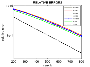
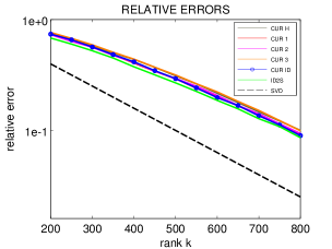
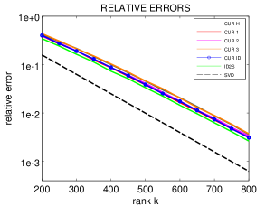
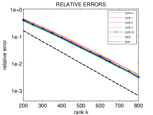
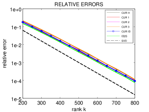
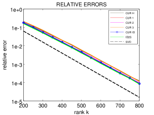
Figure 1: Relative errors for differently conditioned matrices approximated with various algorithms. Left: fat matrices ($1000\times 3000$), right: thin matrices ($3000\times 1000$). Top to bottom: faster drop off of logspaced singular values.

Our first set of test matrices (“Set 1”) involves matrices $\bm{\mathsf{A}}$ of size $1000\times 3000$, of the form $\bm{\mathsf{A}}=\bm{\mathsf{U}}\,\bm{\mathsf{D}}\,\bm{\mathsf{V}}^{*}$ where $\bm{\mathsf{U}}$ and $\bm{\mathsf{V}}$ are random orthonormal matrices, and $\bm{\mathsf{D}}$ is a diagonal matrix with entries that are logspaced between $1$ and $10^{b}$, for $b=-2,\,-4,\,-6$. The second set (“Set 2”) are simply the transposes of the matrices in Set 1 (so these are matrices of size $3000\times 1000$). Figure 1 plots the median relative errors in the spectral norm between the matrix $\bm{\mathsf{A}}$ and the corresponding factorization (with the error defined as $E=\frac{\|\hat{\bm{\mathsf{A}}}_{k}-\bm{\mathsf{A}}\|}{\|\bm{\mathsf{A}}\|}$ where $\hat{\bm{\mathsf{A}}}_{k}=\bm{\mathsf{C}}\bm{\mathsf{U}}\bm{\mathsf{R}}$ is the corresponding approximation of given rank). We plot median quantities collected over $5$ trials. In addition to the four CUR algorithms, we also include plots for the two sided IDand the SVD of given rank (providing the optimal approximation). Based on the plots, we make three conjectures for matrices conditioned similar to those used in this example (note that CUR-1 performs poorly in some of our other experiments):

• The accuracies of CUR-ID, CUR-1, and CUR-2, are all very similar. CUR-H offers slightly worse approximations.

• The accuracy of CUR-3 is worse than all other algorithms tested.

• The two-sided ID is in every case more accurate than the CUR-factorizations.

Next, in Figure 2, we compare the performance and runtimes of CUR-H, CUR-1, and CUR-2 algorithms with the randomized SVD [10] (which gives close results to the true SVD of given rank but at substantially less cost) and the CUR-ID algorithm using the randomized ID, as described in this text (using $q=2$ in the power sampling scheme (5.3)). This comparison allows us to test algorithms which can be used in practice on large matrices, since they involve randomization. We again use random matrices constructed as above whose singular values are logspaced, ranging from $10^{0}$ to $10^{-3}$, but of larger size: $2000\times 4000$. We notice that the performance with all schemes is similar but the runtime with the randomized CUR-ID algorithm is substantially lower than with the other schemes. The runtime of CUR-1 is substantially greater than of the other schemes. The plotted quantities are again medians over $5$ trials.

In Figure 3, we repeat the experiment using the randomized SVD with the two matrices $\bm{\mathsf{A}}_{1}$ and $\bm{\mathsf{A}}_{2}$ defined in the preprint [18]. The matrices $\bm{\mathsf{A}}_{1},\bm{\mathsf{A}}_{2}\in\mathbb{R}^{300,000\times 300}$ are constructed as follows:

$$\bm{\mathsf{A}}_{1}=\displaystyle\sum_{j=1}^{10}\frac{2}{j}x_{j}y^{T}_{j}+\displaystyle\sum_{j=11}^{300}\frac{1}{j}x_{j}y^{T}_{j}\quad\mbox{and}\quad\bm{\mathsf{A}}_{2}=\displaystyle\sum_{j=1}^{10}\frac{1000}{j}x_{j}y^{T}_{j}+\displaystyle\sum_{j=11}^{300}\frac{1}{j}x_{j}y^{T}_{j},$$

where $x$ and $y$ are sparse vectors with random non-negative entries. One problem with using traditional CUR algorithms for these matrices stems from the fact that the singular values of $\bm{\mathsf{A}}_{1}$ and $\bm{\mathsf{A}}_{2}$ decay rapidly. Due to this, the performance of CUR-1 (and of CUR-3, which we do not show) for these examples is poor. It appears that this is because for these schemes, the rapid decay of the singular values of the input matrix translates into the inversion of ill-conditioned matrices, which adversely effects performance. On the other hand, CUR-ID and CUR-2 offer similar performance, close to the approximate SVD results. In Figure 3, we show the medians of relative errors versus $k$ over $5$ trials.

In Figure 4, we show comparison between absolute errors given by our non-randomized and randomized CUR-ID algorithms and the truncated SVD and QR factorizations in terms of the square of the Frobenius norm and the spectral norm. We use $600\times 600$ test matrices, with varying singular value decay, as before. In particular, we check here if the optimistic bound:

$$\|\bm{\mathsf{A}}-\bm{\mathsf{C}}\bm{\mathsf{U}}\bm{\mathsf{R}}\|_{F}^{2}\leq(1+\epsilon)\|\bm{\mathsf{A}}-\bm{\mathsf{A}}_{k}\|_{F}^{2}\quad\mbox{with}\quad\bm{\mathsf{A}}_{k}=\bm{\mathsf{U}}_{k}\bm{\mathsf{\Sigma}}_{k}\bm{\mathsf{V}}_{k}^{*}$$ (6.1)

from [3] holds with $1<\epsilon<2$ for the non-randomized CUR-ID scheme. For $\epsilon\approx 2$ and $k\ll\min(m,n)$ the bound sometimes holds, but it does not hold for all $k$. Despite this, we may also observe from the bottom row of Figure 4 that for matrices with rapid singular value decay, the CUR-ID error in the spectal norm is sometimes lower even than that of the truncated QR.

In Figure 5, we have an image compression experiment, using CUR-ID and CUR-1,CUR-2, and CUR-H with the full SVD. We take two black and white images (of size $350\times 507$ and $350\times 526$) and transform the matrix using four levels of the $2D$ CDF 97 wavelet transform. We then threshold the result, leaving a sparse $m\times n$ matrix $\bm{\mathsf{M}}$ with about $30\%$ nonzeros (with same dimensions as the original image). Then we go on to construct a low rank CUR approximation of this wavelet thresholded matrix (with $k=\min(m,n)/15$) to further compress the image data. Storing the three matrices $\bm{\mathsf{C}}$, $\bm{\mathsf{U}}$, and $\bm{\mathsf{R}}$ corresponds to storing about $8$ time less nonzeros vs storing $\bm{\mathsf{M}}$. To reconstruct the image from this compressed form, we perform the inverse CDF 97 WT transform on the matrix product $\bm{\mathsf{CUR}}$, which approximates the wavelet thresholded matrix. From the plots, we see that CUR-ID produces a $\bm{\mathsf{U}}$ which has less rapid singular value decay than the $\bm{\mathsf{U}}$ matrix obtained with the CUR-1 and CUR-H algorithms. In particular, the reconstructions obtained with CUR-1 are very poor and the U obtained from this scheme has rapidly decaying singular values, comparable to those of $\bm{\mathsf{M}}$.

Thus, in each case, we observe comparable or even better performance with CUR-ID than with existing CUR algorithms. For large matrices, existing CUR algorithms that rely on the singular vectors must be used in conjunction with an accelerated scheme for computing approximate singular vectors, such as, e.g., the randomized method of [10], or to use CUR-ID with the randomized ID. We find that for random matrices the performance is similar, but CUR-ID is easier to implement and is generally more efficient. Also, as in the case of the imaging example we present, existing CUR algorithms suffer from a badly conditioned $\bm{\mathsf{U}}$ matrix when the original matrix is not well conditioned. The $\bm{\mathsf{U}}$ matrix returned by the CUR-ID algorithm tends to be better conditioned.

Finally, we again remark that optimized codes for the algorithms we propose are available as part of the RSVDPACK software package [20].

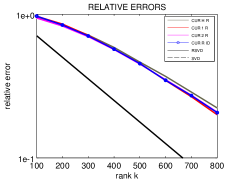
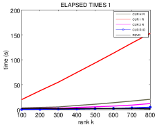
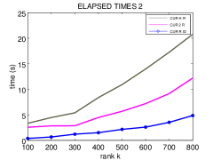
Figure 2: Relative errors and elapsed times for CUR-H,CUR-1,CUR-2 with randomized SVD and CUR-ID with the randomized ID using larger matrices of size $2000\times 4000$. First time plot shows runtimes for all algorithms. Second time plot shows runtimes of CUR-H, CUR-2, and CUR-ID.

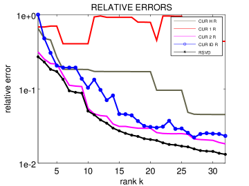
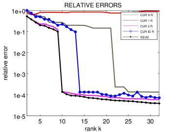
Figure 3: Relative errors versus $k$ for matrices $\bm{\mathsf{A}}_{1}$ (left) and $\bm{\mathsf{A}}_{2}$ (right) from [18] approximated using CUR-H,CUR-1,CUR-2 with randomized SVD and CUR-ID with the randomized ID.

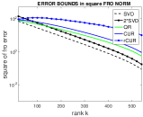
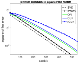
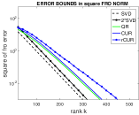
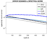
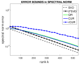
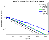
Figure 4: Comparison of absolute error bounds for rank $k$ CUR-ID and CUR-ID with randomization in comparison to truncated rank $k$ SVD and truncated QR decompositions in terms of square Frobenius norm (top) and spectral norm (bottom) for matrices with singular values distributed on a logarithmic scale between $1$ and $10^{-b}$ with $b=1.5,3,4.5$.

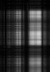
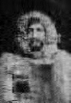
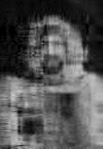
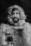
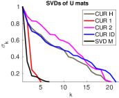
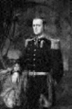
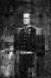
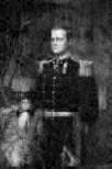
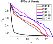
Figure 5: Reconstructed images with CUR compression of the wavelet transformed image. Images resulting from applying Inverse Wavelet transform to matrix product $\bm{\mathsf{CUR}}$ obtained with CUR-1 in column 1, CUR-H in column 2, CUR-2 in column 3, and with CUR-ID in column 4. Column 5 plots: singular value distributions of output $\bm{\mathsf{U}}$ matrices with the different algorithms compared.

7 Conclusions

This paper presents efficient algorithms for computing ID and CUR decompositions. The algorithms are obtained by very minor modifications to the classical pivoted QR factorization. As a result, the new CUR-ID algorithm provides a direct and efficient way to compute the CUR factorization using standard library functions, as provided in, e.g., BLAS and LAPACK.

Numerical tests illustrate that the new algorithm CUR-ID leads to substantially smaller approximation errors than methods that select the rows and columns based on leverage scores only. The accuracy of the new scheme is comparable to existing schemes that rely on additional information in the leading singular vectors, such as, e.g., the DEIM-CUR [18] of Sorensen and Embree, or the “orthogonal top scores” technique in the package rCUR. However, we argue that CUR-ID has a distinct advantage in that it can easily be coded up using existing software packages, and our numerical experiments indicate an advantage in terms of computational speed.

The paper also demonstrates that the two-sided ID is superior to the CUR-decomposition in terms of both approximation errors and conditioning of the factorization. The ID offers the same benefits as the CUR decomposition in terms of data interpretation. However, for very large and very sparse matrices, the CUR decomposition can be more memory efficient than the ID.

Finally, the paper demonstrates that randomization can be used to very substantially accelerate algorithms for computing the ID and CUR-decompositions, including techniques based on leverage scores, the DEIM-CUR algorithm, and the newly proposed CUR-ID. Moreover, randomization can be used to reduce the overall complexity of the CUR-ID-algorithm from $O(mnk)$ to $O(k^{2}m+k^{2}n+mn\log k)$.

Acknowledgement The research reported was supported by the Defense Advanced Projects Research Agency under the contract N66001-13-1-4050, and by the National Science Foundation under contracts 1320652 and 0748488.

References

- [1] E. Anderson, Z. Bai, C. Bischof, S. Blackford, J. Demmel, J. Dongarra, J. Du Croz, A. Greenbaum, S. Hammarling, A. McKenney, and D. Sorensen. LAPACK Users’ Guide. Society for Industrial and Applied Mathematics, Philadelphia, PA, third edition, 1999.
- [2] András Bodor, István Csabai, Michael Mahoney, and Norbert Solymosi. rCUR: an R package for CUR matrix decomposition. BMC Bioinformatics, 13(1), 2012.
- [3] Christos Boutsidis and David P Woodruff. Optimal cur matrix decompositions. In Proceedings of the 46th Annual ACM Symposium on Theory of Computing, pages 353–362. ACM, 2014.
- [4] Tony F. Chan. Rank revealing factorizations. Linear Algebra Appl., 88/89:67–82, 1987.
- [5] Petros Drineas, Michael W. Mahoney, and S. Muthukrishnan. Relative-error matrix decompositions. SIAM J. Matrix Anal. Appl., 30(2):844–881, 2008.
- [6] Carl Eckart and Gale Young. The approximation of one matrix by another of lower rank. Psychometrika, 1(3):211–218, 1936.
- [7] Gene H. Golub and Charles F. Van Loan. Matrix computations. Johns Hopkins Studies in the Mathematical Sciences. Johns Hopkins University Press, Baltimore, MD, fourth edition, 2013.
- [8] Sergei A Goreinov, Eugene E Tyrtyshnikov, and Nickolai L Zamarashkin. A theory of pseudoskeleton approximations. Linear Algebra and its Applications, 261(1):1–21, 1997.
- [9] Ming Gu and Stanley C. Eisenstat. Efficient algorithms for computing a strong rank-revealing qr factorization. SIAM J. Sci. Comput., 17(4):848–869, July 1996.
- [10] N. Halko, P. G. Martinsson, and J. A. Tropp. Finding structure with randomness: probabilistic algorithms for constructing approximate matrix decompositions. SIAM Rev., 53(2):217–288, 2011.
- [11] David C. Hoaglin and Roy E. Welsch. The Hat matrix in regression and ANOVA. The American Statistician, 32(1):17–22, 1978.
- [12] Edo Liberty, Franco Woolfe, Per-Gunnar Martinsson, Vladimir Rokhlin, and Mark Tygert. Randomized algorithms for the low-rank approximation of matrices. Proceedings of the National Academy of Sciences, 104(51):20167–20172, 2007.
- [13] Michael W. Mahoney and Petros Drineas. CUR matrix decompositions for improved data analysis. Proc. Natl. Acad. Sci. USA, 106(3):697–702, 2009. With supplementary material available online.
- [14] Per-Gunnar Martinsson, Vladimir Rokhlin, and Mark Tygert. A randomized algorithm for the approximation of matrices. Technical Report Yale CS research report YALEU/DCS/RR-1361, Yale University, Computer Science Department, 2006.
- [15] Nikola Mitrovic, Muhammad Tayyab Asif, Umer Rasheed, Justin Dauwels, and Patrick Jaillet. CUR decomposition for compression and compressed sensing of large-scale traffic data. Proceedings of the 16th International IEEE Annual Conference on Intelligent Transportation Systems, 2013.
- [16] Vladimir Rokhlin, Arthur Szlam, and Mark Tygert. A randomized algorithm for principal component analysis. SIAM Journal on Matrix Analysis and Applications, 31(3):1100–1124, 2009.
- [17] Tamas Sarlos. Improved approximation algorithms for large matrices via random projections. In 2006 47th Annual IEEE Symposium on Foundations of Computer Science (FOCS’06), pages 143–152. IEEE, 2006.
- [18] D. C. Sorensen and M. Embree. A DEIM Induced CUR Factorization. ArXiv e-prints, July 2014.
- [19] Eugene Tyrtyshnikov. Incomplete cross approximation in the mosaic-skeleton method. Computing, 64(4):367–380, 2000.
- [20] Sergey Voronin and Per-Gunnar Martinsson. Rsvdpack: Subroutines for computing partial singular value decompositions via randomized sampling on single core, multi core, and gpu architectures. arXiv preprint arXiv:1502.05366, 2015.
- [21] Shusen Wang and Zhihua Zhang. Improving CUR matrix decomposition and the Nyström approximation via adaptive sampling. J. Mach. Learn. Res., 14:2729–2769, 2013.
- [22] Franco Woolfe, Edo Liberty, Vladimir Rokhlin, and Mark Tygert. A fast randomized algorithm for the approximation of matrices. Applied and Computational Harmonic Analysis, 25(3):335–366, 2008.