DCPT–14/81

December 2014

Form factor relocalisation and interpolating
renormalisation group flows from the staircase model

Patrick Dorey¹, Guy Siviour¹ and Gábor Takács^2,3

¹Department of Mathematical Sciences, Durham University,

South Road, Durham DH1 3LE, United Kingdom

²MTA-BME “Momentum” Statistical Field Theory Research Group,

1111 Budapest, Budafoki út 8, Hungary

³Department of Theoretical Physics,

Budapest University of Technology and Economics,

1111 Budapest, Budafoki út 8, Hungary

E-mails:

p.e.dorey@durham.ac.uk, gbsiviour@gmail.com, takacsg@eik.bme.hu

We investigate the staircase model, introduced by Aliosha Zamolodchikov through an analytic continuation of the sinh-Gordon S-matrix to describe interpolating flows between minimal models of conformal field theory in two dimensions. Applying the form factor expansion and the $c$-theorem, we show that the resulting $c$-function has the same physical content as that found by Zamolodchikov from the thermodynamic Bethe Ansatz. This turns out to be a consequence of a nontrivial underlying mechanism, which leads to an interesting localisation pattern for the spectral integrals giving the multi-particle contributions. We demonstrate several aspects of this form factor relocalisation, which suggests a novel approach to the construction of form factors and spectral sums in integrable renormalisation group flows with non-diagonal scattering.

1 Introduction: the staircase models

Of all integrable two-dimensional quantum field theories admitting a Lagrangian description, the sinh-Gordon model is the simplest to define. Nevertheless its properties continue to surprise, and it is far from being completely understood. In 1991, in a paper that circulated for many years in preprint form before it was finally published in 2006 [1], Aliosha Zamolodchikov pointed out a further curious feature: the S-matrix of the model admits an interesting continuation from its self-dual point to certain complex values of the coupling. The S-matrix remains real-analytic, being real for purely-imaginary values of the rapidity, but acquires a couple of ‘resonance poles’ located just off the physical sheet. As a scattering theory this continued S-matrix appears to make sense, even though the Lagrangian description of the resulting theory is somewhat obscure. Zamolodchikov chose instead to study the properties of the model via the thermodynamic Bethe ansatz (TBA) method, which gives access to the finite-volume ground-state energy of a quantum field theory taking as its only input the exact S-matrix. This revealed an intriguing structure: as a parameter $\vartheta_{0}$ encoding the ‘distance’ of the continued S-matrix from the self-dual point was taken to infinity, the ground-state energy found by plugging the continued S-matrix into the TBA exhibited a sequence of scaling behaviours approximating with increasing accuracy those of the minimal conformal field theories ${\cal M}_{p}$, one after the other. The crossovers between these regions approximated, again with increasing accuracy as $\vartheta_{0}$ increased, the ${\cal M}_{p}\to{\cal M}_{p-1}$ interpolating flows that had previously been found perturbatively in [2, 3] and analysed exactly using the TBA in [4, 5].

Zamolodchikov interpreted these results as suggesting the existence of a family of integrable quantum field theories with what he dubbed ‘roaming’ renormalisation group (RG) trajectories, passing close by each of the minimal models in turn before finally flowing to massive theories in the far infrared. The general idea is illustrated in figure 1 below; each black dot represents an RG fixed point described by a conformal field theory, and the larger the parameter $\vartheta_{0}$ becomes, the nearer the trajectory passes to each fixed point, and the longer it spends there. In the immediate neighbourhood of each fixed point, the model can be described by a combination of a relevant ($\phi_{13}$) and an irrelevant ($\phi_{31}$) perturbations of the corresponding conformal field theory, a picture which was subsequently verified perturbatively to be consistent with the multiply-hopping flows by Lässig [6].

$$\begin{array}[]{c}\leavevmode\resizebox{284.52756pt}{}{ \begin{picture}(0.0,0.0)\includegraphics{Stairflow.pdf}\end{picture}\begin{picture}(8333.0,3198.0)(2686.0,-5053.0)\put(6901.0,-2086.0){\makebox(0.0,0.0)[lb]{\smash{{{\color[rgb]{0,0,0}Increasing $\Theta_{0}$}}}}} \end{picture} }\end{array}$$

Figure 1: A collection of roaming renormalisation group flows, parameterised by $\vartheta_{0}$

Zamolodchikov’s paper led to a series of generalisations [7, 8, 9, 10], with even more elaborate one-parameter families of RG flows emerging from proposed sets of TBA equations, each visiting infinitely-many fixed points in a suitable limit. Similar behaviours were then predicted for the Homogeneous Sine-Gordon (HSG) models [11] and then confirmed by a TBA analysis [12, 13], though in these cases the number of fixed points visited is always finite. The pattern in all cases is of successive hops between a sequence of conformal field theories with decreasing central charges, punctuated by ever-longer ‘pauses’, or plateaux, near to each conformal field theory. For this reason the roaming theories are often called staircase models.

Given the ubiquity of the roaming phenomenon, it seems worthwhile to understand it in more depth, in particular to gather more evidence as to whether the roaming trajectories encode the properties of bona fide local quantum field theories, or are merely mathematical artefacts of the conjectured TBA equations. Further motivation comes from the fact that the S-matrices associated with the roaming trajectories are often far simpler than those of the interpolating flows that they ultimately come to approximate: for example, Zamolodchikov’s original staircase S-matrix is diagonal, while the massless S-matrices associated with the ${\cal M}_{p}\to{\cal M}_{p-1}$ interpolating flows [14] are non-diagonal and significantly more complicated. This has recently been used to conjecture exact equations describing combined bulk and boundary flows between minimal models [15], confirming and extending previous perturbative results [16].

In this paper we consider Zamolodchikov’s staircase model not through the TBA approach, but rather via the form factors that follow from its S-matrix. These give access to (Sasha) Zamolodchikov’s $c$-function [17] for the model, which we find through both numerical and analytical treatments behaves exactly as expected in the $\vartheta_{0}\to\infty$ limit. For the HSG models, the form factor expansion of Zamolodchikov’s $c$-function was studied numerically in [18, 19] (see also section 7 of [13]), and the evidence found therein for a roaming behaviour was an important motivation for our work. However these earlier papers did not provide an analytic explanation for the observed phenomena, something which is of independent interest. In particular, the staircase limit allows us to extract a set of ‘effective’ form factors for the interpolating flows. For the tricritical Ising to Ising flow these reproduce the diagonal massless form factors found by Defino, Mussardo and Simonetti [20], while for flows further up the staircase an interesting picture incorporating extra ‘magnonic’ contributions emerges, hinting at further universal structures in the general form-factor description of perturbed conformal field theories.

In the next section recall some further details of Zamolodchikov’s staircase model and its treatment via the TBA. In section 3 we review the form factor approach and present some numerical results concerning the form factor treatment of the staircase limit. These results are supported by analytic arguments in section 4, while section 5 concludes the paper with some speculations and suggestions for further work.

2 A short review of the staircase TBA system

The sinh-Gordon model is a theory of a single scalar field $\Phi$, with a classical action depending on a mass scale $M$ and coupling $b$:

$$\mathcal{A}=\int d^{2}x\left(\frac{1}{2}\partial_{\mu}\Phi\partial^{\mu}\Phi-\frac{M^{2}}{b^{2}}\cosh b\Phi\right)\;.$$ (2.1)

The model is integrable, with one of the simplest non-trivial exact S-matrices known: in terms of the parameter $\gamma:=\pi b^{2}/(8\pi+b^{2})$, it is

$$S(\theta)=\frac{\sinh\theta-i\sin\gamma}{\sinh\theta+i\sin\gamma}\;.$$ (2.2)

This function has a pair of zeros at $i\gamma$ and $i(\pi{-}\gamma)$ in the physical strip of the complex rapidity plane, and no physical-strip poles; as $b$ varies from $0$ to $\infty$, $\gamma$ moves from $0$ to $\pi$ and the zeros swap over, reflecting the strong-weak coupling duality of the model under $b\to 1/b$, $\gamma\to\pi-\gamma$. The situation is depicted in figure 2.

$$\begin{array}[]{c}\includegraphics[width=180.0pt]{shGS.pdf}\end{array}$$

Figure 2: The analytic structure of the sinh-Gordon S-matrix: there are two zeros on the physical strip $0\leq\Im m\,\theta\leq\pi$, and two poles on the unphysical strip $-\pi\leq\Im m\,\theta\leq 0$.

The roaming S-matrix is obtained from (2.2) by analytically continuing away from the self-dual point $\gamma=\pi/2$, setting

$$\gamma=\frac{\pi}{2}\pm i\vartheta_{0}$$ (2.3)

with $\vartheta_{0}$ real, and letting $\vartheta_{0}$ tend to infinity in the staircase limit. The resulting S-matrix is depicted in figure 3. It is still real-analytic, but now has a pair of forward and crossed channel ‘resonance poles’ on the unphysical sheet, with real parts $\pm\vartheta_{0}$.

$$\begin{array}[]{c}\includegraphics[width=180.0pt]{shGScont.pdf}\end{array}$$

Figure 3: The S-matrix continuation from sinh-Gordon to staircase: the zeros and poles move a distance $\pm\vartheta_{0}$ parallel to the real axis from their positions at the self-dual point.

Whether this continuation makes sense at the level of the action (2.1) is an open question (though see some speculations in the final section of [8]). However as an abstract S-matrix encoding the scattering of asymptotic multiparticle states there are no immediate problems, and under the assumption that this is the S-matrix of underlying massive field theory one can try to discover further properties of this theory using standard methods of integrable models, in particular the TBA and form-factor approaches.

The TBA gives the ground-state energy $E_{0}(R)$ of an integrable QFT on a circle of circumference $R$ in terms of the solutions of one or more non-linear integral (TBA) equations. For a theory with a single massive particle of mass $m$, such as the sinh-Gordon or staircase model, there is just one TBA equation, for a function $\varepsilon(\theta)$ known as the pseudoenergy:

$$\varepsilon(\theta)=r\cosh(\theta)-\int_{\mathbb{R}}\phi(\theta-\theta^{\prime})L(\theta^{\prime})\,d\theta^{\prime}$$ (2.4)

where $L(\theta)=\log(1+e^{-\varepsilon(\theta)})$, $\phi(\theta)=-\frac{i}{2\pi}\frac{d}{d\theta}\log S(\theta)$, and $r=MR$ is the dimensionless system size in units of $1/M$, the correlation length. The ground-state energy is then expressed in terms of a scaling function $c_{\rm eff}(r)$ known as the effective central charge,

$$E_{0}(R)=-\frac{\pi}{6R}\,c_{\rm eff}(r)\,,$$ (2.5)

as

$$c_{\rm eff}(r)=\frac{3}{\pi^{2}}\int_{\mathbb{R}}r\cosh(\theta)L(\theta)\,d\theta\,.$$ (2.6)

For a unitary conformal field theory with central charge $c$, the scaling of the ground-state energy is such that $c_{\rm eff}(r)$ is a constant, equal to $c$. On the other hand, if a theory not conformal but at some length-scale $r$ is close to a conformal field theory, then $c_{\rm eff}(r)$ near that same value of $r$ should be close to the corresponding central charge. For example, as $r\to 0$ the effective central charge of a conformal field theory perturbed by some relevant operator should tend to the central charge of the unperturbed model; but more generally, any pause in the evolution of $c_{\rm eff}(r)$ at an intermediate scale is evidence that the renormalisation group trajectory of the model is passing close by a CFT, with central charge equal to the approximately-constant value of $c_{\rm eff}(r)$ at that scale.

For the staircase model, this is exactly what Zamolodchikov observed. Plots of $c_{\rm eff}$ as a function of $\log(r)$ show the same UV and IR limits as those for the sinh-Gordon model, namely $1$, the central charge of a single free boson, and $0$, the infrared value always found in a theory with no massless degrees of freedom at long distances. But as $\vartheta_{0}$ grows they acquire an increasingly-pronounced series of plateaux at intermediate scales, of widths $\vartheta_{0}/2$. The heights of these plateaux are the central charges of the unitary $c<1$ minimal models, as illustrated in figure 4. These plots imply precisely the RG flows sketched in figure 1 above, with the increasing length of RG time spent on each plateau indicating that the corresponding RG trajectories get nearer and nearer to the RG fixed points as $\vartheta_{0}$ increases.

$$\begin{array}[]{cc}\vartheta_{0}=0:&\quad\parbox[c]{180.0pt}{\includegraphics[height=60.0pt]{shGflow_0.pdf}}\\ \vartheta_{0}=10:&\quad\parbox[c]{180.0pt}{\includegraphics[height=60.0pt]{shGflow_10.pdf}}\\[3.0pt] \vartheta_{0}=20:&\quad\parbox[c]{180.0pt}{\includegraphics[height=60.0pt]{shGflow_20.pdf}}\end{array}$$

Figure 4: The effective central charge of the staircase model for various values of $\vartheta_{0}$.

To understand how this pattern emerges from the TBA equation (2.4), consider the form of the ‘kernel function’ $\phi(\theta)$, which in terms of the parameter $\vartheta_{0}$ is

$$\phi(\theta)=\frac{1}{2\pi\cosh(\theta+\vartheta_{0})}+\frac{1}{2\pi\cosh(\theta-\vartheta_{0})}~{}.$$ (2.7)

When $\vartheta_{0}$ is large this function ‘relocalises’ into a pair of disconnected peaks of width of order 1, situated at $\theta=\pm\vartheta_{0}$ on the real axis, as shown in figure 5.

$$\begin{array}[]{c}\includegraphics[width=180.0pt]{phicont.pdf}\end{array}$$

Figure 5: The TBA kernel function $\phi(\theta)$ for the staircase model.

In turn, the relocalised kernel means that the integral in the TBA equation (2.4) couples $\varepsilon(\theta)$ not to $\varepsilon(\theta^{\prime})$ with $\theta^{\prime}\approx\theta$, but rather to its values at $\theta^{\prime}\approx\theta\pm\vartheta_{0}$. However one must also consider the effect of the driving term $r\cosh(\theta)$ in the TBA equation: for $|\theta|\gg\log(1/r)$ this dominates, causing $\varepsilon(\theta)$ to be large and $L(\theta)$ small. Nontrivial behaviour of $\varepsilon(\theta)$ therefore only occurs in the region $-\log(1/r)\lessapprox\theta\lessapprox\log(1/r)$, and this behaviour depends crucially on how many times the shift $\vartheta_{0}$ fits into this interval. This number changes whenever $2\log(1/r)\approx(k{-}1)\vartheta_{0}$, or $\log(r)\approx-(k{-}1)\vartheta_{0}/2$, explaining the additional steps in the staircase seen in figure 4.

Note that to see the limiting behaviour of $c_{\rm eff}(r)$ on any individual step, it is not enough simply to take $\vartheta_{0}$ to infinity: $r$ must be rescaled to zero simultaneously, otherwise the step will be missed. More precisely, to see the $k^{\rm th}$ step, set

$$r=\tilde{r}\,e^{-(k{-}1)\vartheta_{0}/2}$$ (2.8)

and then let $\vartheta_{0}$ tend to infinity with $\tilde{r}$ remaining finite. In this limit the TBA equation couples the neighbourhood $\theta\approx\log(1/r)\approx(k{-}1)\vartheta_{0}/2$ to $\theta\approx(k{-}3)\vartheta_{0}/2$, which is in turn coupled to $\theta\approx(k{-}1)\vartheta_{0}/2$ and to $\theta\approx(k{-}5)\vartheta_{0}/2$ and so on. As $\vartheta_{0}$ grows these neighbourhoods separate, and $\varepsilon(\theta)$ is best described by introducing a sequence of ‘effective’ pseudoenergies, one for each neighbourhood. As explained in detail in [8], as $\vartheta_{0}\to\infty$ the equations governing these effective pseudoenergies and also the resulting function $c_{\rm eff}(\tilde{r})$ become exactly the massless TBA equations introduced by Zamolodchikov in [4, 5], confirming that, at least as far as the evolution of the effective central charge is concerned, the limiting flow of the staircase model is indeed the sequence of ${\cal M}_{p}\to{\cal M}_{p-1}$ flows, with step $k$ corresponding to $p=k+2$.

In the following we will show that a similar story holds for the form factors. The details are a little more intricate, but the basic idea of relocalisation of integrals, coupled with a form of double-scaling limit involving $r$ and $\vartheta_{0}$ to expose the individual steps, is the same.

3 Some form factor phenomenology

3.1 Form factors, Zamolodchikov’s $c$-theorem and Cardy’s sum rule

An alternative scale-dependent observable to the finite-size ground-state energy is the correlation function of two operators separated by a distance $R$. In a conformal field theory this will scale as a power of $R$; otherwise if in some regime the theory is close to a CFT, then approximate power-law scaling should be observed. However, rather than look for this behaviour directly, Sasha Zamolodchikov pointed out that the correlation functions of the components of the energy-momentum tensor can be used to construct a quantity – the Zamolodchikov $c$-function $c(R)$ [17] – which is constant for a CFT, equal to the theory’s central charge, and which for unitary non-conformal field theories is a decreasing function of $R$. More precisely, we have

$$\frac{dc(R)}{dR}=-{\textstyle\frac{3}{2}}R^{3}\langle\Theta(R)\Theta(0)\rangle\;.$$ (3.1)

where $\Theta$ is the trace of the energy-momentum tensor. As stressed by Cardy, it is useful to integrate this last formula to yield the sum rule [21]:

$$c(R)=c(\infty)+{\textstyle\frac{3}{2}}\int_{R}^{\infty}\!dR^{\prime}\,(R^{\prime})^{3}\langle\Theta(R^{\prime})\Theta(0)\rangle\,.$$ (3.2)

In general $c(R)$ is not the same as the effective central charge discussed in the last section, but the two functions agree for critical models, and are equally effective as tools to analyse an RG flow.

Form factors allow general correlation functions, and in particular those appearing in (3.2), to be expressed as an infinite sum of multiple integrals; and for an integrable QFT the integrands can be determined exactly, at least in principle, once the S-matrix is known. In a theory with a single massive particle of mass $m$ and $n$-particle asymptotic states $|\theta_{1},\dots\theta_{n}\rangle$ with rapidities $\theta_{1}$…$\theta_{n}$, the form factors of the trace of the energy-momentum tensor $\Theta(x)$ are defined as

$$F^{\Theta}_{n}=\langle 0|\Theta(0)|\theta_{1},\dots\theta_{n}\rangle\,.$$ (3.3)

The two-point function of $\Theta$ can be expressed in terms of these form factors by inserting a complete set of states:

$$\langle\Theta(R)\Theta(0)\rangle=\sum_{n=0}^{\infty}\int_{\mathbb{R}^{n}}\!\frac{d\theta_{1}\dots d\theta_{n}}{(2\pi)^{n}n!}|F_{n}^{\Theta}(\theta_{1}\dots\theta_{n})|^{2}\,e^{-mR\sum_{i=1}^{n}\cosh\theta_{i}}.$$ (3.4)

Substituting this expansion into (3.2) and using the fact that for a massive field theory $c(\infty)=0$, the value of the $c$-function is

$$c(r)=3\sum_{n=0}^{\infty}\int_{\mathbb{R}^{n}}\!\frac{d\theta_{1}\dots d\theta_{n}}{(2\pi)^{n}(n!)}\,\frac{6+6rE+3r^{2}E^{2}+r^{3}E^{3}}{2E^{4}}\,|m^{-2}F_{n}^{\Theta}(\theta_{1}\dots\theta_{n})|^{2}\,e^{-rE}\;,$$ (3.5)

where $r=mR$ now denotes the separation of the fields in the two-point functions defining $c(r)$ in units of the correlation length, and the dimensionless ‘energy’ $E$ is

$$E=\sum_{i=1}^{n}\cosh\theta_{i}\;.$$ (3.6)

From now on we use units in which $m=1$, and focus on the sinh-Gordon and staircase models. For ease of reference, some key formulae for the sinh-Gordon form factors together with their most important properties are provided in appendix A.

3.2 Brute force numerics

Under the roaming continuation (2.3), $\sin\gamma$ is replaced by $\cosh\vartheta_{0}$ and $\vartheta_{0}$ is then taken to infinity. Continuing the exact form factors and evaluating the form factor sum rule (3.5) numerically for large values $\vartheta_{0}$, we can check whether the roaming behaviours of the TBA results are also seen in correlation functions.

3.2.1 The Ising flow

If $r$ is held fixed and nonzero as the limit $\vartheta_{0}\rightarrow\infty$ is taken, then all rapidity integrals in (3.5) are effectively confined to a finite (and $\vartheta_{0}$-independent) region by the factor $e^{-rE}$. In such a region the form factors (A.17) of $\Theta$ have the limits

$$F_{2}^{\Theta}(\theta_{1},\theta_{2})=-2\pi i\sinh\frac{\theta_{1}-\theta_{2}}{2}$$

$$F_{n}^{\Theta}(\theta_{1},\dots,\theta_{n})=0\quad\mathrm{for}\quad n\neq 2\;,$$ (3.7)

which coincide with the form factors for the Ising model a.k.a. the free massive Majorana fermion. From (3.5) one obtains [22]

$$\lim_{r\to 0}\left[\lim_{\vartheta_{0}\to\infty}c(r,\vartheta_{0})\,\right]=\frac{1}{2}\;,$$ (3.8)

which is the correct value for an Ising fixed point in the ultraviolet.

3.2.2 Flow from tricritical to critical Ising

To obtain the next step in the staircase, a simple $\vartheta_{0}\rightarrow\infty$ limit is not sufficient. Instead, one must retain the full expressions for the form factors and evaluate the sum rule for a large but fixed value of $\vartheta_{0}$, varying the parameter $r$. The result is shown in figure 6: to obtain the second step we added the 4-particle contributions which contribute a central charge difference $\Delta c=0.19767\dots$ (the result is terminated at the last accurately known digit). It is expected that the second plateau must be at the tricritical Ising value $c=7/10$ so the exact value must be $\Delta c=0.2$; as demonstrated later, the rest of the central charge difference is accounted for by terms with more than 4 particles.

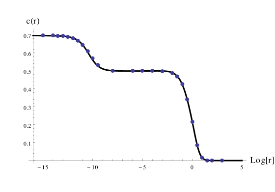
Figure 6: The first two steps of the staircase for $\vartheta_{0}=20$, including 2 and 4 particle contributions. The dots show the result of numerical integration, while the curve is a fit by an appropriate rational function of $r$.

Note that the first step from the Ising model with $c=1/2$ appears at $\log r\approx 0$, while the second one is centred at $\log r=\vartheta_{0}/2$, which explains why it cannot be seen in a naive $\vartheta_{0}\rightarrow\infty$ limit. This is a general pattern: the $k^{\mathrm{th}}$ step, approximating the flow ${\mathcal{M}}_{p}\rightarrow{\mathcal{M}}_{p-1}$ with $p=k+2$ when $\vartheta_{0}$ is large, is centred at

$$\log r=(k-1)\frac{\vartheta_{0}}{2}\;.$$ (3.9)

This behaviour is in full agreement with that of the TBA system discussed in Section 2.

However, higher steps are much harder to calculate to a good accuracy as the integrals are difficult even for sophisticated multi-dimensional integration algorithms. The underlying reasons are the growing dimensionality of the integrals, the growing ranges of rapidities which must be considered when evaluating these integrals, and the progressively more complex shapes of the regions within these ranges where the integrand is significantly different from zero. To improve this situation, it is necessary to understand the nature of the regions to which the integral eventually localises for large values of $\vartheta_{0}$.

3.3 Cells and localisation

The simplest strategy is to divide up the integration space into cells with a hypercubic shape of size $\vartheta_{0}/2$, with centres on a hypercubic lattice with the same spacing. This choice is suggested by the fact that the $e^{-rE}$ factor in the integrand restricts all rapidity integrals to the ranges $-\log(1/r)\lessapprox\theta_{i}\lessapprox\log(1/r)$, while the steps are expected to occur each time $\log(1/r)$ passes an integer multiple of $\vartheta_{0}/2$. An analytic justification will be given in section 4. We introduce the following notation for the hypercubes in rapidity space:

$$[a_{1},\dots,a_{n}]_{\alpha}:=\left\{(\theta_{1},\dots,\theta_{n})\in\mathbb{R}^{n}\,:a_{k}\frac{\vartheta_{0}}{2}-\frac{\alpha}{2}\leq\theta_{k}\leq a_{k}\frac{\vartheta_{0}}{2}+\frac{\alpha}{2}\;,\;k=1,\dots,n\right\}\;,$$ (3.10)

where the integers $a_{k}$ describe the centre of the cell, while $\alpha$ allows for varying its size, with $\alpha=\vartheta_{0}/2$ corresponding to a full elementary cell of the lattice.

It is easy to see that cells differing by symmetry transformations generated by permutations of the centre coordinates $a_{1},\dots,a_{n}$, and by changing their signs simultaneously contribute the same amount, therefore it is enough to evaluate a representative for each sets of equivalent cells. A cell is in normal form if $a_{1}<0$ and the sequence $a_{1},\dots,a_{n}$ is monotonically increasing; each equivalence class of cells can be obtained by applying the symmetries to a cell of normal form.

Performing numerics with the above settings, the following key observations can be made:

1. While increasing $\vartheta_{0}$ gives more accurate values for the steps, especially for higher ones, for each cell $[a_{1},\dots,a_{n}]_{\alpha}$ its contribution is essentially saturated by $\alpha$ of order 1, which stays the same as $\vartheta_{0}$ increases. Therefore the index $\alpha$ is omitted from now on, and the contribution of cell $[a_{1},\dots,a_{n}]$ is always understood to be the saturated value.

2. The contribution to the $k^{\rm th}$ step starts at particle number $n=2k$. It is also interesting to note that the bulk of the contribution is already obtained from this level.

3. Especially for higher steps, the number of potential cells is very large, but only a few of them contribute significantly. For the first four steps and up to 8 particles we list the contributing cells in Table 1. The contributions of ’significant’ cells tends to a constant, while the contributions of others decrease to $0$ in the large $\vartheta_{0}$ limit. Numerically it can be inferred that the asymptotic values of the cell contributions (whether zero or finite) are approached exponentially fast in $\vartheta_{0}$.

Step	2-particle	4-particle	6-particle	8-particle
1	$[0,0]$	–	–	–
2	–	$[-1,-1,1,1]$	$[-1,-1,-1,-1,1,1]$	$[-1,-1,1,1,1,1,1,1]$
				$[-1,-1,-1,-1,1,1,1,1]$
3	–	–	$[-2,-2,0,0,2,2]$	$[-2,-2,0,0,0,0,2,2]$
				$[-2,-2,-2,-2,0,0,2,2]$
4	–	–	–	$[-3,-3,-1,-1,1,1,3,3]$

Table 1: Table of contributing cells up to 8 particles. For each class, we only give a cell of normal form generating them; the rest can be obtained by permuting the integers or changing their signs.

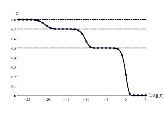
Figure 7: The first three steps of the staircase for $\vartheta_{0}=20$, including 2,4,6 and 8 particle contributions. The dots show the result of numerical integration, the curve is a fit by an appropriate rational function of $r$ to the numerical integration results, while the horizontal lines show the central charges of the first three minimal models.

Using the localisation of the integration, it is possible to obtain a much more accurate result for the flow, as well as to include the third step as shown in figure 7. The plateau values which we obtain are $c=0.5$ (exact), $c=0.6999\dots$ and $c=0.799\dots$ where we terminate the results with the last accurate digit; these are all in good agreement with the minimal model predictions. For the fourth step, the 8-particle contribution (for $\vartheta_{0}=20$) is $\Delta c=0.0470\dots$, while the total expected difference between the corresponding minimal models is $\Delta c=4/70=0.05714\dots$. Again, the majority of the central charge difference arises at the first level that contributes to the given step; however reliable numerical evaluation of higher many-particle integrals proved too difficult, preventing the reconstruction of this step to better accuracy, even using the help of localisation.

The pattern in Table 1 leads us to formulate the following

Theorem R (relocalisation):

The cells contributing to the $k$th step have the following normal form:

$$[a_{1},a_{1},\dots,a_{p},a_{p}]\;:\;p\geq k\;,\;-a_{1}=a_{p}=k-1\;,\;a_{k}-a_{k-1}=0\;\mathrm{or}\;2$$ (3.11)

In the following section we prove this statement using analytic considerations.

4 The form factor integrals in the staircase limit

4.1 Scaling with the distance parameter $r$

To understand the behaviour of the $c$-function, we start by considering the explicit $r$-dependence of the integrand in the c-theorem sum rule (3.5).

The factor

$$e^{-rE}=\prod\limits_{i=1}^{n}e^{-r\cosh\theta_{i}}$$ (4.1)

is the most dominant and the simplest to analyze. Each subfactor obeys

$$e^{-r\cosh\theta_{i}}=\begin{cases}1&|\theta_{i}|\ll-\log r\\ 0&|\theta_{i}|\gg-\log r\end{cases}\;,$$ (4.2)

with the transitional region of $|\theta_{i}|$ around $-\log r$ having a thickness of $O(1)$, i.e. it does not scale with the relevant parameters $\log r$ or $\vartheta_{0}$. This means at a given value of $r$, the contributing region is essentially the hypercube

$$|\theta_{i}|\leq-\log r+O(1)\;,$$ (4.3)

where the $O(1)$ term indicates that the contribution decays in a double exponential way outside the hypercube. Note that all the other terms in the integrand (including the form factors) have at most exponential behaviour in rapidities, so they cannot counteract this behaviour.

In conclusion, for the $k$th step located at

$$-\log r=(k-1)\vartheta_{0}\;,$$ (4.4)

the above considerations imply that contributing cells have coordinates $[a_{1},\dots,a_{n}]$ such that

$$|a_{i}|\leq k-1\quad\mathrm{for}\;i=1,\dots,n\,.$$ (4.5)

4.2 Behaviour of the form factors

We now wish to examine the form factors of the trace of the energy momentum tensor (A.17) in the roaming limit (2.3). Using the Lukyanov representation (A.14) one obtains

$$P_{n}^{(1)}\left(\theta_{1},\dots,\theta_{n}\right)=$$

$$\qquad\sum_{\{\alpha_{j}=\pm 1\}}\left\{\left(\prod_{j=1}^{n}\alpha_{j}e^{-\alpha_{j}(\vartheta_{0}+i\pi/2)}\right)\prod_{r<s}\left(1-i\frac{\alpha_{r}{-}\alpha_{s}}{2}\frac{\cosh\vartheta_{0}}{\sinh\left(\theta_{r}{-}\theta_{s}\right)}\right)\right\}\;.$$ (4.6)

To identify the relevant limiting behaviour we will need let $\vartheta_{0}\to\infty$ in this expression while simultaneously taking suitable rapidity differences to infinity, so as to capture the relocalised contributions from the various cells identified in theorem R of the previous section. These ‘double scaling’ limits are significantly more delicate than those leading to the cluster property (A.15) [23], in which certain rapidity differences are taken to infinity at fixed coupling, and their discussion will take up most of the rest of this section.

4.2.1 Asymptotics of the minimal form factor and normalisation constants

As a preliminary step, we need the asymptotic behaviour of the minimal form factor, which can be written as

$$f(\theta)=\mathcal{N}R(\theta)\;,$$ (4.7)

with

$$R(\theta)=\exp\left[8\int_{0}^{\infty}\frac{dt}{t}\sin^{2}\left(\frac{t(i\pi-\theta)}{2\pi}\right)\frac{\sinh\frac{t\gamma}{2\pi}\sinh(1-\frac{\gamma}{\pi})\frac{t}{2}\sinh\frac{t}{2}}{\sinh^{2}t}\right]\;.$$ (4.8)

Explicit calculation shows that leading asymptotic behaviour of this function is given by

$$R(\theta+k\vartheta_{0}) \mathop{\longrightarrow}\limits_{\vartheta_{0}\rightarrow 0} \begin{cases}-i\sinh\theta/2&k=0\\ e^{\vartheta_{0}/2}\rho(\theta)&k=+1\\ e^{\vartheta_{0}/2}\bar{\rho}(\theta)&k=-1\\ \frac{1}{2}e^{\vartheta_{0}/2}&|k|>1\end{cases}\;,$$ (4.9)

where

$$\rho(\theta) = \frac{1-i}{4}2^{1/4}e^{-K/\pi}e^{\theta/4}\exp\left(-\int_{0}^{\infty}\frac{dt}{t}\frac{\sin^{2}\left(\frac{t(i\pi-\theta)}{2\pi}\right)}{\sinh t\cosh\frac{t}{2}}\right)\;,$$

$$\bar{\rho}(\theta) = \frac{1+i}{4}2^{1/4}e^{-K/\pi}e^{-\theta/4}\exp\left(-\int_{0}^{\infty}\frac{dt}{t}\frac{\sin^{2}\left(\frac{t(i\pi-\theta)}{2\pi}\right)}{\sinh t\cosh\frac{t}{2}}\right)\;,$$ (4.10)

while

$$K=0.915966\dots$$ (4.11)

denotes Catalan’s constant, and

$$\rho(\infty)=\bar{\rho}(-\infty) =\frac{1}{2}$$

$$\rho(-\infty)=\bar{\rho}(\infty) =0\;.$$ (4.12)

In addition, the normalisation $\mathcal{N}$ factor behaves as

$$\mathcal{N} \sim 2e^{-\vartheta_{0}/2}\;,$$ (4.13)

and consequently

$$F_{2}^{(1)}(0,i\pi)\sim-2e^{\vartheta_{0}}\;.$$ (4.14)

4.2.2 Naive power counting

Let us write

$$\theta_{i}=\theta_{i}^{\prime}+t_{i}\vartheta_{0}\;,$$ (4.15)

where $\left|\theta_{i}^{\prime}\right|$ is kept finite as $\vartheta_{0}\rightarrow\infty$. This corresponds to the observation in section 3.3 that the rapidity integration domain can be split into cells $[a_{1},\dots,a_{n}]$. Due to Lorentz invariance (A.2), the form factors only depend on rapidity differences, and according to the form factor equation (A.3), exchanging two rapidities gives just a phase factor. Therefore for the form factor part of the discussion we can perform a global shift and reshuffling of the rapdities to render the $t_{i}$ ordered and positive, with $t_{1}=1$:

$$1=t_{1}\leq\dots\leq t_{n}\;.$$ (4.16)

For a cell of normal form $[a_{1},\dots,a_{n}]$ the corresponding $\vec{t}$ is given by

$$t_{i}=(a_{i}-a_{1})/2+1\quad i=1,\dots,n\;;$$ (4.17)

we will refer to such a cell as being of type $\vec{t}$. Furthermore, the asymptotic behaviour depends only on

$$t_{ij}=t_{i}-t_{j}=(a_{i}-a_{j})/2\;.$$ (4.18)

Since our numerical studies showed that the cell coordinates $[a_{1},\dots,a_{n}]$ of contributing cells are integers of the same parity, we now make the following

Assumption I (integrality):

all the $t_{i}$ are integers. Since $t_{1}$ is fixed to $1$, this is equivalent to

$$t_{ij}\in\mathbb{Z}\;.$$ (4.19)

In Section 4.5 the validity of this assumption will be demonstrated by analytic considerations.

The large-$\vartheta_{0}$ asymptotic behaviour of the form factors in a cell of type $\vec{t}$ is characterised by an exponent $\omega(\vec{t}\>)$ defined as

$$F_{n}^{\Theta}\left(\theta_{1},\dots,\theta_{n}\right)\sim e^{\omega(\vec{t}\>)\vartheta_{0}}$$ (4.20)

or, more precisely

$$\omega(\vec{t}\>):=\lim\limits_{\vartheta_{0}\rightarrow\infty}\frac{1}{\vartheta_{0}}\log F_{n}^{\Theta}\left(\theta_{1}^{\prime}+t_{1}\vartheta_{0},\dots,\theta_{n}^{\prime}+t_{n}\vartheta_{0}\right)\;.$$ (4.21)

Using (A.14), (4.9) and (4.14) one can write

$$\omega(\vec{t}\>)=-1-\frac{n}{4}+\omega_{P}(\vec{t}\>)+\omega_{F}(\vec{t}\>)\;,$$ (4.22)

where the constant $-1$ comes from normalizing by $F_{2}(0,i\pi)$, the term $\omega_{F}(\vec{t}\>)$ is the contribution of the minimal form factors, which can be written as

$$\omega_{F}(\vec{t}\>)=\sum_{<i,j>}\min\left(0,\frac{|t_{ij}|-1}{2}\right)\;,$$ (4.23)

while $\omega_{P}(\vec{t}\>)$ is the asymptotic behaviour of the function $P^{(1)}_{n}$ defined in (4.6).

4.2.3 Upper estimate for $\omega_{P}$

The form factor polynomial $P_{n}^{(1)}$ (4.6) is the sum of $2^{n}$ terms of the form

$$\left(\prod_{j=1}^{n}\alpha_{j}e^{-\alpha_{j}(\vartheta_{0}+i\pi/2)}\right)\prod_{k<j}\left(1-i\frac{\alpha_{k}-\alpha_{j}}{2}\frac{\cosh\vartheta_{0}}{\sinh\left(\theta_{k}-\theta_{j}\right)}\right)\sim e^{\omega_{P}(\vec{\alpha},\vec{t}\>)\vartheta_{0}}\;,$$ (4.24)

where $\omega_{P}(\vec{\alpha},\vec{t}\>)$ is the exponent characterizing the asymptotic behaviour of these terms for each value of $\vec{\alpha}$. Then the following inequality

$$\omega_{P}(\vec{t}\>)\leq\tilde{\omega}_{P}(\vec{t}\>)=\max_{\vec{\alpha}}\omega_{P}(\vec{\alpha},\vec{t}\>)$$ (4.25)

provides an upper estimate for the asymptotic behaviour.

To analyze the $\vec{\alpha}$ dependence we can start with the case

$$\alpha_{1}=\dots=\alpha_{n}=-1\;,$$ (4.26)

for which we obtain

$$\tilde{\omega}_{P}(\vec{\alpha},\vec{t}\>)=n\;.$$ (4.27)

We can then consider the effect of flipping some of the $\alpha_{k}$ from $-1$ to $+1$. It is convenient to introduce a notation in which $\vec{t}$ is parameterised by $N$ blocks of lengths $p_{k}$, $k=1,\dots,N$ such that in the $k$th block the components of $\vec{t}$ are equal to a constant value $v_{k}$:

$$\vec{t}=(\underbrace{v_{1}\dots v_{1}}_{p_{1}},\underbrace{v_{2}\dots v_{2}}_{p_{2}},\dots,\underbrace{v_{N}\dots v_{N}}_{p_{N}})\;,$$ (4.28)

where $v_{N}=\max\vec{t}$, $v_{1}<v_{2}<\dots<v_{N}$ and

$$\sum_{k=1}^{N}p_{k}=n\;.$$ (4.29)

Let us consider the case when there are $r_{1}$ instances of $\vec{\alpha}$ components equal to $+1$ in the first block, $r_{2}$ in the second etc. In terms of $\tilde{\omega}_{P}(\vec{\alpha},\vec{t}\>)$, each such flip comes with a “cost” of $-2$ from the prefactor in the $\vec{\alpha}$-term, while flips in the same block also make “gains” of $+1$ for by “activating” some of the $\cosh\vartheta_{0}$ terms. The number of such activated terms is given by the number of $+1,-1$ pairs inside the blocks, so we obtain

$$\tilde{\omega}_{P}(\vec{\alpha},\vec{t}\>)=n+\sum_{k=1}^{N}(-2r_{k}+(p_{k}-r_{k})r_{k})\;.$$ (4.30)

Since the contributions of the blocks are independent, we can maximise the terms separately:

$$-2r_{k}+(p_{k}-r_{k})r_{k}\quad\mbox{ is maximal when }\quad r_{k}=\left[\frac{p_{k}-2}{2}\right]\;.$$ (4.31)

The end result is

$$\tilde{\omega}_{P}(\vec{t}\>) = n+\sum_{k=1}^{N}\left[\left(\frac{p_{k}-2}{2}\right)^{2}-\frac{\delta_{k}^{2}}{4}\right]$$ (4.32)

$$\delta_{k}=\begin{cases}0&p_{k}\;\mathrm{even}\\ 1&p_{k}\;\mathrm{odd}\end{cases}\;.$$

4.2.4 Upper estimate for $\omega$ and dominant cells

Substituting (4.32) and (4.23) into (4.22), the end result for the upper estimate $\tilde{\omega}$ is

$$\omega(\vec{t}\>)\leq\tilde{\omega}(\vec{t}\>)=-1+\frac{3n}{4}+\sum_{k=1}^{N}\left(\frac{p_{k}-2}{2}\right)^{2}-\sum_{k=1}^{N}\frac{\delta_{k}^{2}}{4}+\sum_{\left\langle i,j\right\rangle}\min\left(0,\frac{|t_{ij}|-1}{2}\right)\;,$$ (4.33)

where $\left\langle i,j\right\rangle$ denotes an (unordered) pair of indices between $1$ and $n$. Using the integrality assumption $t_{ij}\in\mathbb{Z}$ the last term can be computed explicitly, since the summands are all $0$ except when $t_{ij}=0$, which is when $\left\langle i,j\right\rangle$ is a pair from inside the same block. Such pairs contribute $-1/2$, so

$$\tilde{\omega}(\vec{t}\>) = -1+\frac{3n}{4}+\sum_{k=1}^{N}\left[\left(\frac{p_{k}-2}{2}\right)^{2}-\frac{p_{k}(p_{k}-1)}{4}\right]-\sum_{k=1}^{N}\frac{\delta_{k}^{2}}{4}$$ (4.34)

$$= -1+\sum_{k=1}^{N}\left(\frac{3}{4}p_{k}+\frac{4-3p_{k}}{4}\right)-\sum_{k=1}^{N}\frac{\delta_{k}^{2}}{4}$$

$$= -1+N-\sum_{k=1}^{N}\frac{\delta_{k}^{2}}{4}\;.$$

This is surprisingly simple: the end result is just the number of blocks minus 1, with a negative correction for odd blocks.

In the following section we show that the relevant issue is to find the dominant blocks for a fixed value of

$$D(\vec{t}\>)=\max\vec{t}-\min\vec{t}\;,$$ (4.35)

which measures the real space “length” of the sequence $\vec{t}$. In this case the way to maximise the number of blocks is to minimise the steps between blocks, so for the dominant cells integers in adjacent blocks differ by $1$:

$$v_{k+1}-v_{k}=1\;.$$ (4.36)

The total number of blocks is then given by $N=D(\vec{t}\>)+1$. To further maximise the contribution all block lengths should be chosen even. As a result, for any fixed value of $D(\vec{t}\>)$ the dominant contributions comes from cells which have the largest possible number of blocks, all of which are even.

Note that so far we have only obtained an upper limit for the scaling exponent $\omega(\vec{t}\>)$. This can be taken into account by writing the true exponent in the form

$$\omega(\vec{t}\>)=\tilde{\omega}(\vec{t}\>)+\Delta\omega(\vec{t}\>)\;,$$ (4.37)

where

$$\Delta\omega(\vec{t}\>)=\omega_{P}(\vec{t}\>)-\tilde{\omega}_{P}(\vec{t}\>)\leq 0$$ (4.38)

will be called the anomaly term. This arises from potential cancellations between terms with different $\vec{\alpha}$, to which we return later in Section 4.4.

4.3 $c$-function in the roaming limit: proof of Theorem R

Now let us examine the $c$-function contributions. Let us take a cell $[a_{1},\dots,a_{n}]$ of normal form, i.e.

$$a_{1}\leq\dots\leq a_{n}\;,$$ (4.39)

and recall that the corresponding $t$ sequence is

$$t_{i}=(a_{i}-a_{1})/2+1\quad i=1,\dots,n\;.$$ (4.40)

The upper limit for the form factor exponent is given by

$${\omega}(\vec{t}\>)\leq\tilde{\omega}(\vec{t}\>)=N-1\;,$$ (4.41)

where $N$ is the number of blocks in $\vec{t}$. For a given cell to contribute to $c(r)$ its coordinates must satisfy

$$\log r\leq a_{1}\leq\dots\leq a_{n}\leq-\log r\;.$$ (4.42)

The contribution of a cell $[\vec{a}]$ satisfying (4.42) to the $c$-function (3.5) is given by

$$\int_{[\vec{a}]}\!\frac{d\theta_{1}\dots d\theta_{n}}{(2\pi)^{n}(n!)}\,\frac{6+6rE+3r^{2}E^{2}+r^{3}E^{3}}{2E^{4}}\,|m^{-2}F_{n}^{\Theta}(\theta_{1}\dots\theta_{n})|^{2}\,e^{-rE}\;.$$ (4.43)

For the values of $r$ when the given cell contributes $rE$ is $O(1)$, i.e. it is bounded by a $\vartheta_{0}$ independent constant when scaling $\vartheta_{0}\rightarrow\infty$ (in fact $rE\lesssim n$). Therefore the scaling power $\zeta(\vec{a})$ of the $c$-function contribution from cell $[\vec{a}]$ can be defined as the behaviour of the integral

$$\int_{[\vec{a}]}\!\frac{d\theta_{1}\dots d\theta_{n}}{(2\pi)^{n}(n!)}\,\frac{|m^{-2}F_{n}^{\Theta}(\theta_{1}\dots\theta_{n})|^{2}}{2E^{4}}\propto e^{\zeta(\vec{a})\vartheta_{0}}$$ (4.44)

or, more precisely

$$\zeta(\vec{a}):=\mathop{\mathrm{lim}}\limits_{\vartheta_{0}\rightarrow\infty}\;\frac{1}{\vartheta_{0}}\log\int_{[\vec{a}]}\!\frac{d\theta_{1}\dots d\theta_{n}}{(2\pi)^{n}(n!)}\,\frac{|m^{-2}F_{n}^{\Theta}(\theta_{1}\dots\theta_{n})|^{2}}{2E^{4}}\;.$$ (4.45)

The behaviour of the form factor depends only the differences $t_{ij}=t_{i}-t_{j}$; however the energy denominator breaks translational invariance in rapidity space. For a given $\vec{t}$ the value of $a_{n}-a_{1}=2(D(\vec{t}\>)-1)$ is fixed, while $a_{1}$ is fixed by the energy denominator, which is minimised when $\mathop{\mathrm{m}ax}\limits_{i}|a_{i}|=a_{n}$ takes the smallest possible value. As a result the maximum contribution is obtained when $a_{1}=-a_{n}$, all other cases being suppressed by powers of $e^{\vartheta_{0}}$. Therefore the cells giving the highest possible contribution have the form

$$[\vec{a}]=[\underbrace{-k+1,\dots,-k+1}_{p_{1}},\underbrace{-k+1,\dots,-k+1}_{p_{2}},\dots,\underbrace{k-1,\dots,k-1}_{p_{k}}]\;,$$ (4.46)

where $k=D(\vec{t}\>)$, each $p_{l}$ is a positive even number, and $(k-1)\vartheta_{0}/2\leq-\log r$. For such a cell the number of blocks is exactly $N=k$ and the energy denominator has the behaviour

$$E^{4}\propto\exp\left\{2(k-1)\vartheta_{0}\right\}\;,$$ (4.47)

so that the contribution of a cell (4.46) to the $c$-function scale with the exponent

$$\zeta(\vec{a})=2\omega(\vec{t}\>)-2(k-1)<2(N-k)=0\;.$$ (4.48)

This shows that the contribution of dominant cells scales to at most a constant when $\vartheta_{0}\rightarrow\infty$. Therefore none of the subdominant cells can give any contributions in this limit. More precisely, since our estimate is only an upper one, it can be stated that cells (4.46) are the only ones which have any chance at all to give a non-vanishing contributions in the roaming limit. However, at this stage we cannot be certain whether all of them contribute. In Section 4.4 below we show that for these cells the anomaly term vanishes, therefore they all contribute in the roaming limit, with the exception of the $k=1$ case, where the only contributing cell is $[0,0]$.

Our result also explains the existence of steps in $c(r)$. Since (under the assumption of integrality) $k$ can only take positive integer values, in the $O(1)$ vicinity of the special values

$$\log r=-\frac{k-1}{2}\vartheta_{0}\;,\quad k=1,2,\dots$$ (4.49)

new cells are switched on, giving rise to the staircase pattern in $c(r)$, with crossovers in the vicinity of the above values of $\log r$, and plateau connecting the crossover regions to each other.

The above argument proves Theorem R stated in section 3.3, provided the integrality assumption $t_{ij}\in\mathbb{Z}$ is taken granted.

4.4 The anomaly term

Recall that so far we only established an upper bound on cell contributions. By considering the scaling anomaly defined in (4.37) this can be refined into an exact result. The anomaly term results from cancellations between terms with different $\vec{\alpha}$ in (4.6), which reduce the exponent of $e^{\vartheta_{0}}$ compared to the naive power counting performed so far. Suppose $\vec{t}$ has the form

$$\vec{t} = (\underbrace{v_{1}\dots v_{1}}_{p_{1}},\underbrace{v_{2}\dots v_{2}}_{p_{2}},\dots,\underbrace{v_{N}\dots v_{N}}_{p_{N}})$$ (4.50)

$$1=v_{1}<v_{2}<\dots<v_{N}\leq n$$

Let us introduce the following classification: an index pair $\left\langle j,k\right\rangle$ is called

1. internal if $|t_{jk}|=0$; this means $j$ and $k$ have $a_{j}=a_{k}$, i.e. they are from inside the same block;

2. strongly linked if $|t_{jk}|=1$;

3. weakly linked if $|t_{jk}|\geq 2$.

The vector $\vec{t}$ can be partitioned into clusters by weak links. A cluster consists of blocks which are separated by strong links; a cluster is called primitive if it consists of a single block. In (4.24) weak links contribute only a factor $1$ in the limit $\vartheta_{0}\rightarrow\infty$, therefore

$$P_{n}^{(1)}\left(\theta_{1},\dots,\theta_{n}\right)\sim$$ (4.51)

$$~{}~{}~{}\prod_{\mbox{\small clusters}\,\mathcal{C}}\,\sum_{\vec{\alpha}\in A(\mathcal{C})}\!\left\{\!\left(\prod_{j\in\mathcal{C}}\alpha_{j}e^{-\alpha_{j}(\vartheta_{0}+i\pi/2)}\!\right)\!\prod_{<j,k>\in\mathcal{C}}\left[\left(1-i\frac{\alpha_{k}{-}\alpha_{j}}{2}\frac{\cosh\vartheta_{0}}{\sinh\left(\theta_{k}{-}\theta_{j}\right)}\right)\right]\right\}\;,$$

where $A(\mathcal{C})$ is the set of $\vec{\alpha}$ configurations inside $\mathcal{C}$. Due to this factorisation property cancellations can only happen within clusters.

We digress a little to discuss the relation of this classification with the form factor cluster property (A.18). In the roaming case (2.3) it can be rewritten as

$$F_{n+m}^{\Theta}\left(\theta_{1}+\Lambda,\dots,\theta_{n}+\Lambda,\theta_{1}^{\prime},\dots,\theta_{m}^{\prime}\right) = \frac{2\cosh\vartheta_{0}}{\pi}F_{n}^{\Theta}\left(\theta_{1},\dots,\theta_{n}\right)F_{m}^{\Theta}\left(\theta_{1}^{\prime},\dots,\theta_{m}^{\prime}\right)$$ (4.52)

$$+O\left(e^{-\Lambda}\right).$$

For $\vartheta_{0}$ finite this leads to a twofold classification of links into internal and weak ones, whereas internal links are those between rapidities separated by finite distance as $\Lambda\rightarrow\infty$, while weak links are those which are between rapidities whose distance grows with $\Lambda$. However, in our case the classification is more refined as $\vartheta_{0}\rightarrow\infty$. This results from the fact that

$$\mathrm{for}\quad|\theta_{k}-\theta_{j}|=\alpha\vartheta_{0}+O(1):\quad\frac{\cosh\vartheta_{0}}{\sinh\left(\theta_{k}{-}\theta_{j}\right)}\rightarrow\begin{cases}\infty&\alpha<1\\ O(1)&\alpha=1\\ 0&\alpha>1\end{cases}\;,$$ (4.53)

which exactly corresponds to the threefold (internal/strong/weak) classification introduced above.

Returning to the anomaly, let us first consider a primitive cluster $\bar{\mathcal{C}}$ of length $p$; the factor corresponding to cluster $\bar{\mathcal{C}}$ is exactly the $p$-particle form factor polynomial in the variables $\theta_{j}$ with $j\in\bar{\mathcal{C}}$, which contributes the power

$$\omega_{\bar{\mathcal{C}}}=\omega_{P}(\underbrace{1\dots 1}_{p})\;.$$ (4.54)

On the other hand from (A.16)

$$\omega_{P}(\underbrace{1\dots 1}_{p})=\omega_{Q}(p)+p\;,$$ (4.55)

where $\omega_{Q}(p)$ is defined by the asymptotics

$$Q_{p}(\theta_{1},\dots\theta_{p})\sim e^{\omega_{Q}(p)\vartheta_{0}}$$ (4.56)

for $\vartheta_{0}\rightarrow\infty$ with $\theta_{i}$ kept finite. The recursion relation (A.10) gives

$$\omega_{Q}(p+2)=\omega_{Q}(p)+p-2\;,$$ (4.57)

and using the value $\omega_{Q}(2)=0$ we obtain

$$\omega_{Q}(p)=\frac{(p-2)^{2}}{4}-\frac{p-2}{2}$$ (4.58)

resulting in

$$\omega_{P}(\underbrace{1\dots 1}_{p})=\frac{(p-2)^{2}}{4}+\frac{p+2}{2}\;.$$ (4.59)

The naive value is given by the $N=1$ case of (4.32)

$$\tilde{\omega}_{P}(\underbrace{1\dots 1}_{p})=p+\frac{(p-2)^{2}}{4}\;.$$ (4.60)

so the anomaly for a single primitive cluster is

$$\Delta\omega(\underbrace{1\dots 1}_{p})=\omega_{P}(\underbrace{1\dots 1}_{p})-\tilde{\omega}_{P}(\underbrace{1\dots 1}_{p})=-\frac{p-2}{2}\;.$$ (4.61)

Non-primitive clusters are composed of several blocks connected by strong links, which are of order $1$ and depend on relative rapidities between the clusters, which can take any finite value. As a result, they upset the cancellation between terms with different $\vec{\alpha}$ which is responsible for the anomaly. Therefore only primitive clusters contribute to the anomaly, and their contributions are additive due to the factorisation between clusters.

Our final result for the anomaly is

$$\Delta\omega(\vec{t}\>)=~{}-\!\!\!\!\!\!\sum_{{\genfrac{}{}{0.0pt}{}{\mathcal{C}\mbox{\tiny: primitive}}{\mbox{\tiny cluster}}}}\!\!\!\frac{\mbox{length}(\mathcal{C})-2}{2}\;.$$ (4.62)

Let us examine the sequences

$$\vec{t}=(\underbrace{1\dots 1}_{p_{1}},\underbrace{2\dots 2}_{p_{2}},\dots,\underbrace{k\dots k}_{p_{k}})\;,$$ (4.63)

which the naive power counting identified as the ones potentially contributing to the $c$-function at step $k$. For $k\geq 2$ $\vec{t}$ is composed of a single non-primitive cluster, therefore the anomaly is zero. At step $k=1$ the naively contributing cells form a primitive cluster

$$\vec{t}=(\underbrace{1\dots 1}_{p})\;,$$ (4.64)

and their $e^{\vartheta_{0}}$ power in the $c$-function is

$$\zeta(\vec{t}\>)=2\omega(\vec{t}\>)-2(k-1)=2\Delta\omega(\vec{t}\>)=-p+2\;.$$ (4.65)

This agrees with the fact that the first step (corresponding to the Ising model) receives only two-particle ($p=2$) contributions.

4.5 Eliminating the integrality assumption

We recall that in the derivation of the contributing cells, our crucial starting assumption (inferred from the numerics) was that we can parameterise the relevant regions in the rapidity space as

$$\theta_{i}=\theta_{i}^{\prime}+t_{i}\vartheta_{0}\;,$$ (4.66)

where

$$t_{ij}=t_{i}-t_{j}$$ (4.67)

are integers, while $\theta_{i}^{\prime}$ are finite while $\vartheta_{0}\rightarrow\infty$. Because of this limit, however, vast parts of the rapidity space are not covered by the arguments. Here we argue that these domains do not contribute to tha $c$-function (3.5) in the limit $\vartheta_{0}\rightarrow\infty$.

To begin with, we note that the cells satisfying the rule formulated in Theorem R all contribute a finite amount in the limit $\vartheta_{0}\rightarrow\infty$. Therefore to eliminate any other possibilities it is enough to demonstrate their suppression relative to these cells by a factor which vanishes in the same limit. In fact, what can be demonstrated is that relaxing assumption I introduces a suppression which is exponential in $\vartheta_{0}$.

Following the conventions introduced in Section 4.2.3 we use the block notation

$$\vec{t} = (\underbrace{v_{1}\dots v_{1}}_{p_{1}},\underbrace{v_{2}\dots v_{2}}_{p_{2}},\dots,\underbrace{v_{N}\dots v_{N}}_{p_{N}})$$ (4.68)

$$v_{1}<v_{2}<\dots<v_{N}$$

$$t_{ij}=t_{i}-t_{j}\qquad v_{ij}=v_{i}-v_{j}\;,$$

and also recall the definition of the “length” of $\vec{t}$:

$$D(\vec{t}\>)=v_{N}-v_{1}\;.$$ (4.69)

The results (4.23) and (4.30) can be rewritten to take into account that the $t_{ij}$ are not necessarily integers. The contribution (4.23) of the minimal form factors can be written as

$$\omega_{F}(\vec{\alpha},\vec{t}\>)=-\sum_{k=1}^{N}\frac{p_{k}(p_{k}-1)}{4}+\sum_{<i,j>:|v_{ij}|<1}p_{i}p_{j}\frac{|v_{ij}|-1}{2}\;,$$ (4.70)

where the last term is a correction by the minimal form factors for which $t_{ij}<1$. The generalisation of (4.30) is

$$\tilde{\omega}_{P}(\vec{\alpha},\vec{t}\>)=n+\sum_{k=1}^{N}(-2r_{k}+(p_{k}-r_{k})r_{k})+\sum_{<i,j>:|v_{ij}|<1}\left(r_{i}(p_{j}-r_{j})+r_{j}(p_{i}-r_{i})\right)(1-|v_{ij}|)\;,$$ (4.71)

where the last term is contributed by inter-block links that are “activated” by the choice of $\vec{\alpha}$. Substituting these contributions into (4.22) results in

$$\tilde{\omega}(\vec{\alpha},\vec{t}\>)=-1+\frac{3n}{4}+\sum_{k=1}^{N}(-2r_{k}+(p_{k}-r_{k})r_{k})-\sum_{k=1}^{N}\frac{p_{k}(p_{k}-1)}{4}$$

$$-\sum_{<i,j>}\frac{1-|v_{ij}|}{2}(p_{i}-2r_{i})(p_{j}-2r_{j})\theta(1-|v_{ij}|)\;.$$ (4.72)

Introducing the notation $s_{k}=p_{k}-2r_{k}$:

$$\tilde{\omega}(\vec{\alpha},\vec{t}\>) = -1+\frac{3n}{4}+\frac{1}{4}\sum_{k=1}^{N}p_{k}^{2}-4p_{k}-\frac{1}{4}\sum_{k=1}^{N}\left(s_{k}^{2}-4s_{k}\right)-\sum_{k=1}^{N}\frac{p_{k}(p_{k}-1)}{4}-\sum_{<i,j>}\frac{A_{ij}}{2}s_{i}s_{j}$$ (4.73)

$$= -1+N-\frac{1}{4}\sum_{k=1}^{N}\left(s_{k}-2\right)^{2}-\sum_{<i,j>}\frac{A_{ij}}{2}s_{i}s_{j}\;,$$

where the matrix $A$ is defined as

$$A_{ij}=\frac{1-|v_{ij}|}{2}\theta(1-|v_{ij}|)\;.$$ (4.74)

It is important to note that $0\leq A_{ij}<1/2$ for all $i,j$. The maximum value of $\tilde{\omega}$ is determined by the condition

$$-\frac{1}{2}s_{k}+1-\sum_{j}A_{kj}s_{j}=0\;,$$ (4.75)

which can be written in matrix notation as

$$(2A+1)\vec{s} = \vec{\rho}$$

where $$\vec{\rho}=(2,2,\dots,2)\;.$$ (4.76)

Note that $s_{k}$ must be integer with the same parity as $p_{k}$; if any of the $s_{k}$ is not then it must be “rounded” to one of the nearest such values. However, such a rounding can only decrease $\tilde{\omega}(\vec{t}\>)$ so for an upper estimate it can be neglected, which often simplifies the arguments.

Let us first assume that $A=0$. Then the solution is $s_{k}=2$, which gives

$$\tilde{\omega}(\vec{t}\>)=-1+N\;.$$ (4.77)

However, this value is only allowed when all the $p_{k}$ are even, since for odd $p_{k}$ only odd $s_{k}$ is possible. As a result the rounded values for $\vec{s}$ are

$$\vec{s} = \vec{\rho}+\vec{\delta}$$ (4.78)

$$\delta_{k}=\begin{cases}0&p_{k}\mbox{ even}\\ \pm 1&p_{k}\mbox{ odd}\end{cases}\;.$$

leading to

$$\tilde{\omega}(\vec{t}\>)=-1+N-\frac{1}{4}\sum_{k=1}^{N}\delta_{k}^{2}\;,$$ (4.79)

which coincides with our previous result (4.34). Using the same argument for cell centring as in Section 4.3, the $c$-function exponent is

$$\zeta(\vec{a}) \leq 2(\tilde{\omega}(\vec{t}\>)-D(\vec{t}\>))$$

where $$a_{k}=t_{k}-t_{1}-\frac{D(\vec{t}\>)}{2}\;.$$ (4.80)

In order to maximise this it is necessary that $\delta_{k}=0$, i.e. all blocks must be even and to minimise $D(\vec{t}\>)$ with the assumption $A=0$ one must have

$$v_{k+1}-v_{k}=1\;,$$ (4.81)

so our original results are recovered.

In fact, even for the case $A\neq 0$, if there is any gap $v_{k+1}-v_{k}$ between subsequent blocks that is larger than $1$ then it can always be decreased to $1$ without changing $\tilde{\omega}(\vec{t}\>)$, but gaining in the final exponent $\zeta$ by decreasing $D(\vec{t}\>)$, i.e. by “shortening”. So we can proceed by assuming that

$$\left|v_{k+1}-v_{k}\right|\leq 1\mbox{ for all }k\;.$$ (4.82)

For the general case $A\neq 0$, the solution for $\vec{s}$ is

$$\vec{s}_{*}=(1+2A)^{-1}\vec{\rho}$$ (4.83)

provided $(1+2A)$ is invertible, and the maximum value of $\tilde{\omega}$ is given by

$$\tilde{\omega}(\vec{t}\>) = -1+N-\frac{1}{4}(\vec{s}_{*}-\vec{\rho})\cdot(\vec{s}_{*}-\vec{\rho})-\frac{1}{2}\vec{s}_{*}A\vec{s}_{*}$$ (4.84)

$$= -1+N-\frac{1}{2}\vec{\rho}\frac{A}{1+2A}\vec{\rho}$$

$$= -1+N-\frac{1}{2}\vec{\rho}A\vec{s}_{*}\;.$$

4.5.1 Maximum shortening

Our formalism can be checked by looking at the case of maximum shortening:

$$|v_{k+1}-v_{k}|=0\quad\forall\;k\;,$$ (4.85)

i.e. the blocks are eventually joined into a large single one with the length being minimal i.e. $D(\vec{t}\>)=0$. In this case

$$A_{ij}=(1-\delta_{ij})/2\;.$$ (4.86)

In this case the solution for $\vec{s}\;$ is not unique due to the fact that $1+2A$ is a singular matrix: any vector whose elements sum to $2$ works

$$\sum_{i=1}^{N}s_{i}=2\;.$$ (4.87)

This is in accordance with the overall picture, as for the single large block there is a single $s$ parameter, which is exactly

$$s=\sum_{i=1}^{N}s_{i}$$ (4.88)

and must be equal to $2$. One can explicitly evaluate

$$\tilde{\omega} = -1+N-\frac{1}{2}\vec{\rho}\cdot A\cdot\vec{s}$$ (4.89)

$$= -1+N-\frac{1}{4}\sum_{i,j}\rho_{i}(1-\delta_{ij})s_{j}$$

$$= -1+N-\frac{1}{2}(N-1)\sum_{j}s_{j}$$

$$= 0\;$$

which is the correct result for a single block.

Maximum shortening can also arise in parts of the sequence $\vec{t}$ with some if the inter-block gaps being $0$. Suppose that $v_{k,k+1}=0$; for any given $k$; then

$$A_{k,k+1} = \frac{1}{2}$$

$$A_{i,k} = A_{i,k+1}\qquad i\neq k,k+1\;,$$ (4.90)

and the relevant terms in the expression (4.73) for $\tilde{\omega}$ are combined together due to the identity

$$-\frac{1}{4}(s_{k}-2)^{2}-\frac{1}{4}(s_{k+1}-2)^{2}-\frac{A_{k,k+1}}{2}s_{k}s_{k+1}=-\frac{1}{4}(s_{k}+s_{k+1}-2)^{2}-1\;,$$ (4.91)

where the $-1$ corresponds to the decreasing the number of the blocks $N$ to $N-1$. In case of more than one zero gaps this reasoning can be applied iteratively.

4.5.2 The case of small $A$

Note that

$$A_{k,k-1} = A_{k-1,k}=\frac{1-(v_{k}-v_{k-1})}{2}$$

$$A_{kl} \geq 0\qquad|k-l|\neq 1\;,$$ (4.92)

therefore the length $D(\vec{t}\>)$ can be estimated as

$$D(\vec{t}\>) = v_{N}-v_{1}=\sum_{k=1}^{N-1}v_{k}-v_{k-1}\geq-\sum_{i,j}A_{ij}+N-1$$ (4.93)

$$= -\frac{1}{4}\vec{\rho}A\vec{\rho}+N-1\;.$$

Then our upper estimate of $c$-function exponent becomes

$$\zeta(\vec{t}\>)\leq 2(\tilde{\omega}(\vec{t}\>)-D(\vec{t}\>))\leq-\frac{1}{2}\vec{\rho}\frac{2A}{1+2A}\vec{\rho}+\frac{1}{2}\vec{\rho}A\vec{\rho}\;,$$ (4.94)

which can be simplified to

$$\zeta(\vec{t}\>)\leq-\frac{1}{2}\vec{\rho}A\frac{1-2A}{1+2A}\vec{\rho}=-\frac{1}{2}\vec{\rho}A\vec{\rho}+O(A^{2})\;.$$ (4.95)

The leading term is definitely negative, therefore for small deviations from integrality the $c$-function exponent is negative.

4.5.3 The case of small shift

Suppose now that

$$\vec{s}_{*}=(1+2A)^{-1}\vec{\rho}$$ (4.96)

is still close enough to $\vec{\rho}\;$ so that its rounding is identical to the $A=0$ case (4.78). This always happens if $A$ is small enough; however, this is not limited to the approximation used in (4.95). In this case

$$\tilde{\omega}(\vec{t}\>)\leq-1+N-\frac{1}{2}\vec{\rho}A(\vec{\rho}+\vec{\delta)}-\frac{1}{4}\vec{\delta}^{2}\;,$$ (4.97)

and using

$$D(\vec{t}\>)\geq-\frac{1}{4}\vec{\rho}A\vec{\rho}+N-1$$ (4.98)

one obtains

$$\zeta(\vec{t}\>)\leq-\frac{1}{4}\vec{\rho}A\vec{\rho}-\frac{1}{2}\vec{\rho}A\vec{\delta}-\frac{1}{4}\vec{\delta}^{2}\;.$$ (4.99)

Recall that $\rho_{k}=2$ and $A_{ij}>0$ therefore the first term is negative; the absolute value of the second term is always smaller than or equal to the first one as $\delta_{k}=\pm 1$. The second term could only cancel the first one when all $\delta_{k}=-1$, but then the last term is (maximally) negative. Therefore we again conclude

$$\zeta(\vec{t}\>)<0$$ (4.100)

whenever $A\neq 0$.

4.5.4 Summary of the arguments for integrality

Our conclusion is that for a cell characterised with a sequence

$$\vec{t}=(\underbrace{v_{1}\dots v_{1}}_{p_{1}},\underbrace{v_{2}\dots v_{2}}_{p_{2}},\dots,\underbrace{v_{N}\dots v_{N}}_{p_{N}})$$ (4.101)

to contribute to the roaming $c$-function

$$v_{k}-v_{k-1}\leq 1$$ (4.102)

must be satisfied. Further, any deviation from exact equality to $1$ decreases $\zeta$ to first order in the deviation matrix $A$, which makes the block’s contribution vanish in the roaming limit. Incidentally, this also explains why the contribution of each cell satisfying the property R (3.11) comes from an $O(1)$ region around each centre. For larger deviations we could prove that they decrease $\zeta$ as long as the optimal value of $\vec{s}\;$ is not shifted from $\vec{\rho}$.

The case of maximum shortening provides an example when decreasing some of the $v_{k}-v_{k-1}$ results in a shift of the optimal value of $\vec{s}\;$ such that one can again have $\zeta=0$. For a full proof for integrality the only thing left to be shown is that these are the only such cases, but for the time being this remains elusive.

We close with an intuitive picture which is essentially the form factor version of the TBA arguments reviewed in Section 2. The sinh-Gordon $S$ matrix (2.2) continued to the roaming trajectory regime (2.3) takes the form

$$S(\theta)=\frac{\sinh\theta-i\cosh\vartheta_{0}}{\sinh\theta+i\cosh\vartheta_{0}}\;.$$ (4.103)

It satisfies

$$\mathop{\mathrm{lim}}\limits_{\vartheta_{0}\rightarrow\infty}S(\theta\pm\vartheta_{0})=\pm\frac{e^{\theta}-i}{e^{\theta}+i}\;,$$ (4.104)

and apart from a finite (i.e. $O(1)$) vicinity of the points $\theta=\pm\vartheta_{0}$, the $S$-matrix is essentially constant:

$$S(\theta)=\begin{cases}-1&|\theta|\ll\vartheta_{0}\\ +1&|\theta|\gg\vartheta_{0}\end{cases}\;.$$ (4.105)

The form factor equations (A.3,A.4,A.5) imply that the dependence of the form factor on the rapidity differences is determined by the $S$-matrix. Given the above properties of the $S$-matrix it is clear that what matters is only whether the $t_{ij}$ (individually) are smaller, larger or exactly equal to $1$.

The asymptotics of $S$ for $|\theta|\gg\vartheta_{0}$ are consistent with the cluster property (A.15), which implies that if any of the $t_{ij}$ is larger than $1$ (but not necessarily an integer), its exact value ceases to have an effect on the asymptotic behaviour of the form factors. The asymptotics of $S$ for $|\theta|\ll\vartheta_{0}$ has a different effect. The fact that $S(0)=-1$ means that the form factors vanish whenever any two of their rapidity arguments are equal, i.e. they obey a Pauli exclusion principle. One then expects that this persists for rapidity differences much smaller than $\vartheta_{0}$. This is indeed true for the minimal form factor function (A.7), which according to the results of Section 4.2.1 behaves as

$$f(\theta)=\begin{cases}0&|\theta|\ll\vartheta_{0}\\ \rho(\theta-\vartheta_{0})&\theta=\vartheta_{0}+O(1)\\ \bar{\rho}(\theta+\vartheta_{0})&\theta=-\vartheta_{0}+O(1)\\ 1&|\theta|\gg\vartheta_{0}\end{cases}$$ (4.106)

for large $\vartheta_{0}$.

One can then visualise the situation in the following way. The $c$-function integrand

$$\frac{6+6rE+3r^{2}E^{2}+r^{3}E^{3}}{2E^{4}}|F_{n}^{\Theta}(\theta_{1},\dots,\theta_{n})|^{2}\,e^{-rE}$$ (4.107)

can be considered as the negative of a potential function for particles positioned at $\theta_{1}$,$\dots$,$\theta_{n}$. The regions contributing to the $c$-function are where the potential is close to being minimal (i.e. the integrand is close to being maximal). Due to the above exclusion principle, there is a short range repulsion between the particles which vanishes when their distance is larger than $\vartheta_{0}$. The $e^{-rE}$ term constrains the particles to an interval defined by $|\theta_{i}|<-\log r$, while the energy denominator tries to squeeze them closer to the origin. So the particles would prefer to be placed at distances of at least $\vartheta_{0}$; with the confining potential provided by the energy denominator, the minimisation of their potential energy results in the formation of “pockets” of size $O(1)$ separated by distances $\vartheta_{0}$, which is exactly the content of the integrality assumption. Once this is realised, one can proceed to find the optimal distribution of particles between the pockets following the method outlined in Sections 4.2 and 4.3, which results in the rule (3.11).

5 Effective magnonic system

Here we show that form factor relocalisation permits the reconstruction of form factors in the massless flows between the minimal models induced by the $\Phi_{1,3}$ perturbation. The basic idea is very simple. Using Theorem R formulated in section 3.3 the c-theorem sum rule (3.5) can be rewritten as a sum over the contributing cells $[a_{1},\dots,a_{n}]$

$$c(r) = 3\sum_{n=0}^{\infty}\sum\limits_{[a_{1},\dots,a_{n}]}\;\int\limits_{[a_{1},\dots,a_{n}]}\!\frac{d\theta_{1}\dots d\theta_{n}}{(2\pi)^{n}(n!)}\,\frac{6+6rE+3r^{2}E^{2}+r^{3}E^{3}}{2E^{4}}\,|m^{-2}F_{n}^{\Theta}(\theta_{1}\dots\theta_{n})|^{2}\,e^{-rE}$$ (5.1)

$$+\dots\;,$$

where the omitted terms decay exponentially with increasing $\vartheta_{0}$.

Each contributing cell can be reparameterised by integration variables $\beta_{i}$ that have the centre of the cell as their origin:

$$\theta_{i}=\beta_{i}+a_{i}\frac{\vartheta_{0}}{2}\qquad i=1,\dots,n\;.$$ (5.2)

Using the rescaling

$$r=\tilde{r}e^{-(k-1)\vartheta_{0}/2}$$ (5.3)

to localise the integral to step $k$ one obtains the $c$-function for the flow corresponding to step $k$ as

$$c_{k}(r) = \lim_{\vartheta_{0}\rightarrow\infty}\sum_{n=0}^{\infty}\sum\limits_{\genfrac{}{}{0.0pt}{}{[a_{1},\dots,a_{n}]}{a_{n}=k-1}}\;\int\limits_{[a_{1},\dots,a_{n}]}\!\frac{d\theta_{1}\dots d\theta_{n}}{(2\pi)^{n}(n!)}\,\Bigg{[}\frac{6+6rE+3r^{2}E^{2}+r^{3}E^{3}}{2E^{4}}\,e^{-rE}$$ (5.4)

$$\times|m^{-2}F_{n}^{\Theta}(\beta_{1}+a_{1}\vartheta_{0}/2,\dots,\beta_{n}+a_{n}\vartheta_{0}/2)|^{2}\Bigg{]}$$

$$E=\sum\limits_{i=1}^{n}\cosh(\beta_{i}+a_{i}\vartheta_{0}/2)\;.$$

where the sum runs over sequences $[a_{1},\dots,a_{n}]$ allowed by the rule expressed in Theorem R. Rewriting the allowed sequences to block notation and relabelling the $\beta_{i}$ accordingly as follows

$$[a_{1},\dots,a_{n}]=[\underbrace{-k+1,\dots,-k+1}_{2p_{-k+1}},\underbrace{-k+3,\dots,-k+3}_{2p_{-k+3}},\dots,\underbrace{k-1,\dots,k-1}_{2p_{k-1}}]$$

$$\{\beta_{1},\dots\,\beta_{n}\}=\{\beta^{(-k+1)}_{1},\dots,\beta^{(-k+1)}_{2p_{-k+1}},\beta^{(-k+3)}_{1},\dots,\beta^{(-k+3)}_{2p_{-k+3}},\dots,\beta^{(k-1)}_{1},\dots,\beta^{(k-1)}_{2p_{k-1}}\}\;,$$ (5.5)

the $c$-function for step $k$ takes the form

$$c_{k}(r) = \sum_{n=0}^{\infty}\sum\limits_{\genfrac{}{}{0.0pt}{}{\{p_{i}\}}{2\sum\limits_{i}p_{i}=n}}\;\frac{1}{n!}\int\limits\!\left(\prod\limits_{i=-k+1}^{k-1}\prod\limits_{j_{i}=1}^{2p_{i}}\frac{d\beta^{(p_{i})}_{j_{i}}}{2\pi}\right)\,\Bigg{[}\frac{6+6\tilde{r}\tilde{E}+3\tilde{r}^{2}\tilde{E}^{2}+\tilde{r}^{3}\tilde{E}^{3}}{2\tilde{E}^{4}}\,e^{-\tilde{r}\tilde{E}}$$ (5.6)

$$\times\left|\mathcal{F}_{\{p_{i}\}}^{\Theta}\left(\beta^{(-k+1)}_{1},\dots,\beta^{(-k+1)}_{2p_{-k+1}},\beta^{(-k+3)}_{1},\dots,\beta^{(-k+3)}_{2p_{-k+3}},\dots,\beta^{(k-1)}_{1},\dots,\beta^{(k-1)}_{2p_{k-1}}\right)\right|^{2}\Bigg{]}$$

$$\tilde{E}=\sum\limits_{i=1}^{2p_{-k+1}}e^{-\beta^{(p_{-k+1})}_{i}}+\sum\limits_{i=1}^{2p_{k-1}}e^{\beta^{(p_{k-1})}_{i}}\;,$$

where $\{p_{i}\}$ is a shorthand for $\{p_{-k+1},p_{-k+3},\dots,p_{k-1}\}$ and

$$\mathcal{F}_{\{p_{i}\}}^{\Theta}\left(\beta^{(-k+1)}_{1},\dots,\beta^{(-k+1)}_{2p_{-k+1}},\beta^{(-k+3)}_{1},\dots,\beta^{(-k+3)}_{2p_{-k+3}},\dots,\beta^{(k-1)}_{1},\dots,\beta^{(k-1)}_{2p_{k-1}}\right)=$$

$$\lim_{\vartheta_{0}\rightarrow\infty}m^{-2}e^{-2(k-1)\vartheta_{0}}F_{n}^{\Theta}(\beta_{1}+a_{1}\vartheta_{0}/2,\dots,\beta_{n}+a_{n}\vartheta_{0}/2)\;,$$ (5.7)

where on the right hand side we returned the original notation for the cell coordinates and the shifted rapidity variables $\beta_{i}$ in order to keep the formula compact.

The result (5.6) has a very compelling interpretation in terms of the massless flow that corresponds to step $k$. Namely, the rapidities $\beta^{(l)}_{i}$ can be thought of as being grouped into $k$ bins corresponding to their upper index. The ones in the leftmost bin correspond to left-moving particles, while the ones in the rightmost bin to right-moving particles, both massless. This is reflected by their contribution to the rescaled dimensionless energy $\tilde{E}$. Note, however, that the rapidities in intermediate bins do not contribute to the energy at all. Recalling that the scattering theory of the massless flow is described by a factorised scattering theory of massless kinks (corresponding to domain walls), one can understand the rapidity variables in the $k-2$ intermediate bins as magnonic degrees of freedom describing the multiplet structure of multi-kink states. Note that the number and the adjacency structure of these bins exactly conforms to the Dynkin diagram encoding the TBA system derived by Zamolodchikov for the corresponding massless flow [5].

Therefore the functions $\mathcal{F}^{\Theta}$ can be interpreted as form factors of the trace of the stress energy tensor (expressed in units $m=1$) along the massless flow in the magnonic basis of multi-kink states. In principle such form factors could be obtained from the form factor bootstrap; however, the non-diagonal nature of kink scattering makes it notoriously difficult to obtain solutions of the bootstrap equations. Indeed, the only nontrivial flow for which the form factor solution is presently known is the case $k=2$ corresponding to the flow from the tricritical to critical Ising model, where the scattering is effectively diagonal and therefore magnons are absent. By a somewhat tedious, but elementary computation it can be shown that the form factors constructed according to (5.7) for $k=2$ indeed match the ones obtained by Delfino et al. [20], up to a phase factor which is irrelevant for the spectral weight.

6 Conclusions

In the present work we have shown how Zamolodchikov’s roaming flows can be analysed via the $c$-theorem, representing the $c$-function as a form factor spectral sum. In particular, we demonstrated that the well-known staircase structure of the free energy obtained from the TBA can be recovered from the $c$-theorem.

We have shown that this is the result of an interesting property of sinh-Gordon form factors under the roaming continuation, which results in a relocalisation of multi-particle contributions to the $c$-function. Our demonstration is in fact an almost complete mathematical proof, the only ingredient not fully proven is the integrality assumption (4.19); however, we presented quite strong evidence that this property holds as well.

The relocalisation property, central to our results, is essentially equivalent to the construction of exact form factors for the trace of energy-momentum tensor in the field theories describing interpolating flows between minimal models. This is a very interesting result given that solving the form factor bootstrap for these flows is a rather nontrivial task due to the non-diagonal nature of the exact $S$-matrix. The scattering matrix in these theories is non-diagonal, which prevents finding the form factors via a general Ansatz involving polynomial recursion relations as in the case of diagonal models. In some field theories with non-diagonal scattering, the form factor bootstrap can still be solved using some ingenious methods (cf. e.g. [24, 25, 26]); however, no generally applicable approach exists. Constructing form factors using relocalisation of simple form factor solutions under a roaming continuation effectively circumvents this problem, and the resulting form factors can be used to compute correlation functions. For the trace of energy-momentum operator this is equivalent to constructing Zamolodchikov’s $c$-function for the flow; however, there is much more potential in the approach, as we discuss below.

One possible extension of our results would be to examine the properties of other form factor solutions, corresponding to exponential operators $e^{\kappa b\Phi}$ with exponents $\kappa\neq\pm 1$. Taking the roaming limit of such form factors, one expects to find the form factors of other relevant local fields of $\Phi_{1,3}$ perturbed minimal conformal field theories, thus giving access to further interesting correlators such as e.g. magnetic susceptibility. The $\Delta$-theorem [23] evaluated as a sum rule over form factors could help in operator identification and also give a more detailed characterisation of the renormalisation group flow by relating the operator contents at the endpoints of the flow.

It is very plausible that the relocalisation property extends to other interesting theories such as homogeneous sine-Gordon models where staircase structures corresponding to resonance spectra have been found [11, 12, 13, 18, 19], and to already known extensions of roaming trajectories [7, 8, 9, 10]. In this connection the association of the form factor structures to Dynkin-like structures is also interesting to investigate and clarify, as they can lead to a classification of form factor solutions for a wide class of scattering theories. Such Dynkin form factors would allow for a direct way to conjecture form factor solutions in the case of non-diagonal scattering. This would be similar in spirit to the Dynkin TBAs of [27]; in fact, based on the present work one expects a deep relation to the structure of TBA diagrams. In particular, note that the form factors constructed via relocalisation account for the non-diagonal nature of scattering theory via magnonic particles, which is exactly analogous to the TBA case.

Acknowledgements

We are grateful to Olalla Castro-Alvaredo, Benjamin Doyon, Luis Miramontes and Fedor Smirnov for useful discussions, and especially to Yaroslav Pugai for suggesting we utilise the Lukyanov representation for the form factors. P.E.D. acknowledges support from the STFC under the Consolidated Grants ST/J000426/1 and ST/L000407/1, G.S. was supported by an STFC studentship, and G.T. was supported by Lendület grant LP2012-50/2014. This research was also supported in part by the Marie Curie network GATIS (gatis.desy.eu) of the European Union’s Seventh Framework Programme FP7/2007-2013/ under REA Grant Agreement No 317089.

Appendix A Exact form factors in sinh-Gordon theory

The form factors of the exponential operators

$$F_{n}^{(\kappa)}(\theta_{1},\theta_{2},\dots,\theta_{n})=\langle 0|e^{\kappa b\Phi}|\theta_{1},\dots,\theta_{n}\rangle$$ (A.1)

in the sinh-Gordon model (2.1) are particular solutions of the following form factor bootstrap equations:

I. Lorentz invariance:

$$F_{n}^{\mathcal{O}}(\theta_{1}+\Lambda,\dots,\theta_{n}+\Lambda)=e^{s_{\mathcal{O}}\Lambda}F_{n}^{\mathcal{O}}(\theta_{1},\dots,\theta_{n})\,;$$ (A.2)

II. Exchange:

$$F_{n}^{\mathcal{O}}(\theta_{1},\dots,\theta_{k},\theta_{k+1},\dots,\theta_{n})=S(\theta_{k}-\theta_{k+1})F_{n}^{\mathcal{O}}(\theta_{1},\dots,\theta_{k+1},\theta_{k},\dots,\theta_{n})\,;$$ (A.3)

III. Cyclic permutation:

$$F_{n}^{\mathcal{O}}(\theta_{1}+2i\pi,\theta_{2},\dots,\theta_{n})=F_{n}^{\mathcal{O}}(\theta_{2},\dots,\theta_{n},\theta_{1})\,;$$ (A.4)

IV. Kinematical singularity

$$-i\mathop{\textrm{Res}}_{\theta=\theta^{{}^{\prime}}}F_{n+2}^{\mathcal{O}}(\theta+i\pi,\theta^{{}^{\prime}},\theta_{1},\dots,\theta_{n})=\left(1-\delta_{i\,j}\prod_{k=1}^{n}S_{i\,i_{k}}(\theta-\theta_{k})\right)F_{n}^{\mathcal{O}}(\theta_{1},\dots,\theta_{n})\,;$$ (A.5)

with Lorentz spin $s_{\mathcal{O}}=0$. The general solution of these equations has the form [28]

$$F_{n}^{(\kappa)}(\theta_{1},\theta_{2},\dots,\theta_{n}) = \mathcal{G}_{\kappa}\left(\frac{4\sin\gamma}{\mathcal{N}}\right)^{n/2}\frac{Q_{n}^{(\kappa)}(x_{1},\dots,x_{n})}{\prod\limits_{r<s}(x_{r}+x_{s})}\prod_{r<s}f(\theta_{r}-\theta_{s})\;,$$ (A.6)

$$x_{r}=e^{\theta_{r}}\;,$$

where the minimal two-particle form factor is

$$f(\theta)=\mathcal{N}\exp\left[8\int_{0}^{\infty}\frac{dt}{t}\sin^{2}\left(\frac{t(i\pi-\theta)}{2\pi}\right)\frac{\sinh\frac{\gamma}{2\pi}\sinh(1-\frac{\gamma}{\pi})\frac{t}{2}\sinh\frac{t}{2}}{\sinh^{2}t}\right]\,.$$ (A.7)

The normalisation constant $\mathcal{N}$, chosen so that $f(\pm\infty)=1$, is

$$\mathcal{N}=\exp\left[-4\int_{0}^{\infty}\frac{dt}{t}\frac{\sinh\frac{\gamma}{2\pi}\sinh(1-\frac{\gamma}{\pi})\frac{t}{2}\sinh\frac{t}{2}}{\sinh^{2}t}\right]$$ (A.8)

and

$$\mathcal{G}_{\kappa}=\langle 0|e^{\kappa b\Phi}|0\rangle$$ (A.9)

is the vacuum expectation value of the field. An exact formula for the expectation values of exponential fields in the sine-Gordon model was obtained in [29], from which the relevant expectation values in the sinh-Gordon theory can be obtained by analytic continuation; however, their explicit forms are not needed in the sequel. The symmetric polynomials $Q_{n}$ satisfy the recursive relations [28]

$$(-1)^{n}Q_{n+2}(-x,x,x_{1},\dots,x_{n})=xD_{n}(x|x_{1},\dots,x_{n})Q_{n}(x_{1},\dots,x_{n})\;,$$ (A.10)

where

$$D_{n}(x|x_{1},\dots,x_{n})=$$

$$\qquad\frac{1}{2\sin\gamma}\sum_{l,k=0}^{n}(-1)^{l}\sin\left((k-l)\gamma\right)x^{2n-l-k}\sigma_{l}^{(n)}(x_{1},\dots,x_{n})\sigma_{k}^{(n)}(x_{1},\dots,x_{n})\;,$$ (A.11)

and $\sigma_{l}^{(n)}$ denotes the elementary symmetric polynomials defined by

$$\prod_{r=1}^{n}(x+x_{r}) = \sum_{l=1}^{n}x^{n-l}\sigma_{l}^{(n)}(x_{1},\dots,x_{n})$$

$$\sigma_{l}^{(n)}\equiv 0 \mbox{if }\>l<0\mbox{ or }l>n\,.$$ (A.12)

For the exponential operators (A.1), the polynomials $Q_{n}$ are given explicitly by the following determinant representation [30]

$$Q_{1}^{(\kappa)} = [\kappa]$$

$$Q_{n}^{(\kappa)} = [\kappa]\det M^{(n)}(k)\qquad n>1$$ (A.13)

$$M_{rs}^{(n)}(\kappa)=[r-s+\kappa]\sigma_{2r-s}^{(n)}(x_{1},\dots,x_{n})\quad r,s=1,\dots,n-1$$

$$[a]=\frac{\sin\,a\gamma}{\sin\gamma}\,.$$

Another useful representation of the same form factor can be obtained from Lukyanov’s result for breather form factors in the sine-Gordon model [31]. Analytic continuation of first breather form factors to imaginary sine-Gordon coupling gives the following result for form factors of exponential operators in sinh-Gordon model:

$$F_{n}^{(\kappa)}\left(\theta_{1},\dots,\theta_{n}\right) =\,\mathcal{G}_{\kappa}\frac{i^{n}}{\left(\mathcal{N}\sin\gamma\right)^{n/2}}P_{n}^{(\kappa)}\left(\theta_{1},\dots,\theta_{n}\right)\prod_{r<s}f(\theta_{r}{-}\theta_{s})\,,$$ (A.14)

$$P_{n}^{(\kappa)}\left(\theta_{1},\dots,\theta_{n}\right) =\sum_{\{\alpha_{j}=\pm 1\}}\left\{\left(\prod_{j=1}^{n}\alpha_{j}e^{-i\alpha_{j}\kappa\gamma}\right)\prod_{r<s}\left(1-i\frac{\alpha_{r}{-}\alpha_{s}}{2}\frac{\sin\gamma}{\sinh\left(\theta_{r}{-}\theta_{s}\right)}\right)\right\}.$$

From this representation it is easy to see that the form factors of exponential operators satisfy the cluster property [23]

$$F_{n+l}^{(\kappa)}\left(\theta_{1}+\Lambda,\dots,\theta_{n}+\Lambda,\theta_{1}^{\prime},\dots,\theta_{l}^{\prime}\right)=\frac{1}{\mathcal{G}_{k}}F_{n}^{(\kappa)}\left(\theta_{1},\dots,\theta_{n}\right)F_{l}^{(\kappa)}\left(\theta_{1}^{\prime},\dots,\theta_{l}^{\prime}\right)+O\left(e^{-\Lambda}\right)$$

$$\;\mathrm{when}\;\Lambda\rightarrow\infty.$$ (A.15)

The identification between the two representations is given by the relation

$$P_{n}^{(\kappa)}\left(\theta_{1},\dots,\theta_{n}\right)=\left(-2i\sin\gamma\right)^{\!n\,}\frac{Q_{n}^{(\kappa)}(e^{\theta_{1}},\dots,e^{\theta_{n}})}{\prod\limits_{r<s}\left(e^{\theta_{r}}+e^{\theta_{s}}\right)}\,.$$ (A.16)

For the $c$-function we need the form factors of the trace of the energy momentum tensor $\Theta$, which is given by [28]

$$F_{n}^{\Theta}\left(\theta_{1},\dots,\theta_{n}\right)=\begin{cases}\frac{2\pi m^{2}}{F_{2}^{(1)}(i\text{$\pi$,0})}F_{n}^{(1)}\left(\theta_{1},\dots,\theta_{n}\right)&\quad n\mbox{ even}\\ 0&\quad n\mbox{ odd}\end{cases}$$ (A.17)

and the cluster property (A.15) can be rewritten as

$$F_{n+l}^{\Theta}\left(\theta_{1}+\Lambda,\dots,\theta_{n}+\Lambda,\theta_{1}^{\prime},\dots,\theta_{l}^{\prime}\right) = \frac{2\sin\gamma}{\pi m^{2}}\,F_{n}^{\Theta}\left(\theta_{1},\dots,\theta_{n}\right)F_{l}^{\Theta}\left(\theta_{1}^{\prime},\dots,\theta_{l}^{\prime}\right)$$ (A.18)

$$+O\left(e^{-\Lambda}\right)\;,$$

provided both $n$ and $l$ are even.

References

- [1] Al.B. Zamolodchikov, ‘Resonance factorized scattering and roaming trajectories’, J. Phys. A 39 (2006) 12847.
- [2] A.B. Zamolodchikov, ‘Renormalization group and perturbation theory near fixed points in two-dimensional field theory’, Sov. J. Nucl. Phys. 46 (1987) 1090 [Yad. Fiz. 46 (1987) 1819].
- [3] A.W.W. Ludwig and J.L. Cardy, ‘Perturbative evaluation of the conformal anomaly at new critical points with applications to random systems’, Nucl. Phys. B 285, 687 (1987).
- [4] Al.B. Zamolodchikov, ‘From tricritical Ising to critical Ising by thermodynamic Bethe ansatz’, Nucl. Phys. B 358 (1991) 524.
- [5] Al.B. Zamolodchikov, ‘Thermodynamic Bethe ansatz for RSOS scattering theories’, Nucl. Phys. B 358 (1991) 497.
- [6] M. Lassig, ‘Multiple crossover phenomena and scale hopping in two-dimensions’, Nucl. Phys. B 380 (1992) 601 [arXiv:hep-th/9112032].
- [7] M.J. Martins, ‘Renormalization group trajectories from resonance factorized S matrices’, Phys. Rev. Lett. 69 (1992) 2461 [arXiv:hep-th/9205024].
- [8] P.E. Dorey and F. Ravanini, ‘Staircase models from affine Toda field theory’, Int. J. Mod. Phys. A 8 (1993) 873 [arXiv:hep-th/9206052].
- [9] M.J. Martins, ‘Analysis of asymptotic conditions in resonance functional hierarchies’, Phys. Lett. B 304 (1993) 111.
- [10] P. Dorey and F. Ravanini, ‘Generalizing the staircase models’, Nucl. Phys. B 406 (1993) 708 [arXiv:hep-th/9211115].
- [11] J.L. Miramontes and C.R. Fernandez-Pousa, ‘Integrable quantum field theories with unstable particles’, Phys. Lett. B 472 (2000) 392 [hep-th/9910218].
- [12] O.A. Castro-Alvaredo, A. Fring, C. Korff and J.L. Miramontes, ‘Thermodynamic Bethe ansatz of the homogeneous sine-Gordon models’, Nucl. Phys. B 575 (2000) 535 [arXiv:hep-th/9912196].
- [13] P. Dorey and J.L. Miramontes, ‘Mass scales and crossover phenomena in the homogeneous sine-Gordon models’, Nucl. Phys. B 697 (2004) 405 [arXiv:hep-th/0405275].
- [14] P. Fendley, H. Saleur and Al.B. Zamolodchikov, ‘Massless flows, 2. The Exact S matrix approach’, Int. J. Mod. Phys. A 8 (1993) 5751 [hep-th/9304051].
- [15] P. Dorey, R. Tateo and R. Wilbourne, ‘Exact g-function flows from the staircase model’, Nucl. Phys. B 843 (2011) 724 [arXiv:1008.1190 [hep-th]].
- [16] S. Fredenhagen, M.R. Gaberdiel and C. Schmidt-Colinet, ‘Bulk flows in Virasoro minimal models with boundaries’, J. Phys. A 42 (2009) 495403 [arXiv:0907.2560 [hep-th]].
- [17] A. B. Zamolodchikov, ‘Irreversibility of the Flux of the Renormalization Group in a 2D Field Theory’, JETP Lett. 43 (1986) 730 [Pisma Zh. Eksp. Teor. Fiz. 43 (1986) 565].
- [18] O.A. Castro-Alvaredo and A. Fring, ‘Renormalization group flow with unstable particles’, Phys. Rev. D 63 (2001) 021701 [hep-th/0008208].
- [19] O.A. Castro-Alvaredo and A. Fring, ‘Decoupling the SU(n)(2) homogeneous Sine-Gordon model’, Phys. Rev. D 64 (2001) 085007 [hep-th/0010262].
- [20] G. Delfino, G. Mussardo and P. Simonetti, ‘Correlation functions along a massless flow’, Phys. Rev. D 51 (1995) 6620 [hep-th/9410117].
- [21] J. L. Cardy, “The Central Charge and Universal Combinations of Amplitudes in Two-dimensional Theories Away From Criticality,” Phys. Rev. Lett. 60 (1988) 2709.
- [22] C. Ahn, G. Delfino and G. Mussardo, ‘Mapping between the sinh-Gordon and Ising models’, Phys. Lett. B 317 (1993) 573 [hep-th/9306103].
- [23] G. Delfino, P. Simonetti and J. L. Cardy, ‘Asymptotic factorization of form-factors in two-dimensional quantum field theory’, Phys. Lett. B 387 (1996) 327-333 [hep-th/9607046].
- [24] F. A. Smirnov, “Form-factors in completely integrable models of quantum field theory,” Adv. Ser. Math. Phys. 14 (1992) 1.
- [25] S. L. Lukyanov, “Free field representation for massive integrable models,” Commun. Math. Phys. 167 (1995) 183 [hep-th/9307196].
- [26] H. M. Babujian, A. Fring, M. Karowski and A. Zapletal, “Exact form-factors in integrable quantum field theories: The Sine-Gordon model,” Nucl. Phys. B 538 (1999) 535 [hep-th/9805185].
- [27] F. Ravanini, R. Tateo and A. Valleriani, “Dynkin TBAs,” Int. J. Mod. Phys. A 8 (1993) 1707 [hep-th/9207040].
- [28] A. Fring, G. Mussardo and P. Simonetti, ‘Form-factors for integrable Lagrangian field theories, the sinh-Gordon theory’, Nucl. Phys. B 393 (1993) 413-441 [hep-th/9211053].
- [29] S.L. Lukyanov and A.B. Zamolodchikov, ‘Exact expectation values of local fields in quantum sine-Gordon model’, Nucl. Phys. B 493 (1997) 571-587 [hep-th/9611238].
- [30] A. Koubek and G. Mussardo, ‘On the operator content of the sinh-Gordon model’, Phys. Lett. B 311 (1993) 193-201 [hep-th/9306044].
- [31] S.L. Lukyanov, ‘Form-factors of exponential fields in the Sine-Gordon model’, Mod. Phys. Lett. A 12 (1997) 2543-2550 [hep-th/9703190].