Exact finite volume expectation values of local operators in excited states

Abstract

We present a conjecture for the exact expression of finite volume expectation values in excited states in integrable quantum field theories, which is an extension of an earlier conjecture to the case of general diagonal factorized scattering with bound states and a nontrivial bootstrap structure. The conjectured expression is a spectral expansion which uses the exact form factors and the excited state thermodynamic Bethe Ansatz as building blocks. The conjecture is proven for the case of the trace of the energy-moment tensor. Concerning its validity for more general operators, we provide numerical evidence using the truncated conformal space approach. It is found that the expansion fails to be well-defined for small values of the volume in cases when the singularity structure of the TBA equations undergoes a non-trivial rearrangement under some critical value of the volume. Despite these shortcomings, the conjectured expression is expected to be valid for all volumes for most of the excited states, and as an expansion above the critical volume for the rest.

1 Introduction

Finite temperature expectation values play an important role in various applications of quantum field theory, and have been intensively studied in recent years in the context of $1+1$ dimensional integrable quantum field theories. For the one-point function a series expansion was conjectured by Leclair and Mussardo in [1], based on the thermodynamic Bethe Ansatz [2] as applied to integrable quantum field theories [3], and the exact form factors from the bootstrap program [4, 5, 6]. Recently, the Leclair-Mussardo series found applications in quantum quenches [7, 8] and the investigations of one-dimensional quantum gases [9, 10, 11].

Another method to obtain finite temperature correlators is based on finite temperature form factors [12, 13]; so far, however, this approach seems limited to free theories such as the Ising model. Other approaches that can be used to construct finite temperature expectation values in integrable models use separation of variables [14, 15], or exploit the hidden Grassmannian/fermionic structure of the XXZ spin chain [16, 17, 18].

In [19, 20] a description of form factors in finite volume was introduced, which was subsequently used to prove the Leclair-Mussardo series [8]. This formalism was also used to compute the finite-temperature two-point function [21, 22], for which a systematic expansion was developed in [23, 24]. Besides further applications to two-point functions in condensed matter systems [25, 26], the finite volume form factor formalism have found numerous other applications, in computing one-point functions in the presence of boundaries [27], in the study of quantum quenches in field theories [28, 29, 30], and in the context of holographic duality [31, 32]. They also provide a useful tool for testing exact form factor solutions obtained from the form factor bootstrap, recently in the boundary [33] and defect [34] settings.

The finite volume form factor formalism introduced in [19, 20] only included the corrections that decay with a power of the volume; exponential corrections were neglected. However, soon after [19, 20] a method was proposed in [35] to construct certain exponential corrections, the so-called $\mu$-terms which are related to the bootstrap fusion between the particles. It was found that these can be very important in determining matrix elements and resonance parameters [36].

However, for integrable quantum field theories one expects that an exact determination of finite volume form factors is also possible. For the Ising model on a lattice this was known before [37, 38]; however, until recently there have been no such results for generic models.

In [39] an extension of the Leclair-Mussardo series was conjectured to describe exact excited state expectation values (a.k.a. diagonal form factors) in finite volume. The methods of [39] apply to theories like the sinh-Gordon model which have no bound states in their bootstrap, and the thermodynamic Bethe Ansatz equations describing excited states in finite volume have a particularly simple structure [40].

In the present work we extend this conjecture to theories with a diagonal factorized scattering that have a nontrivial bootstrap structure. In such models, the excited state levels in finite volumes are described by excited TBA systems of the type introduced in [41, 42, 43]. This conjecture is verified in two ways. First, we show for the trace of stress-energy tensor the conjectured series is equivalent to the result obtained directly from the thermodynamic Bethe Ansatz. Second, we make use of the truncated conformal space approach (TCSA) [44] to get a nontrivial further check of the series. For the latter, we use the methods developed in [45], to which the interested reader is referred to for details.

The outline of the paper is as follows. In Section 2 we introduce our notations and state the conjecture. In section 3 we present the proof that the conjectured series gives the same result as the thermodynamic Bethe Ansatz when evaluated for the trace of the stress-energy tensor. In Section 4 we turn to the so-called $T_{2}$ model used as testing ground, and specify the expansion for the case of the excited state thermodynamic Bethe Ansatz of this particular field theory. The resulting expectation value are then compared to numerical results from the TCSA in Section 5, while Section 6 contains our conclusions and outlook. As the method used for numerically evaluating the connected diagonal form factors contains some non-trivial tricks, and could be useful for other applications, it is presented in Appendix A.

2 Finite volume expectation values in excited states: the conjecture

The Leclair-Mussardo series for the finite volume vacuum expectation value of a local operator in an integrable model with diagonal scattering and $k$ species of massive particles takes the following form [1]:

$$\left\langle\mathcal{O}\right\rangle_{L} = \sum_{n_{1},\dots,n_{k}=0}^{\infty}\left(\prod_{i=1}^{k}n_{i}!\right)^{-1}\int_{-\infty}^{\infty}\prod_{j=1}^{\tilde{N}}\frac{\mathrm{d}\theta_{j}}{2\pi\left[1+e^{\varepsilon_{\beta_{j}}\left(\theta_{j}\right)}\right]}F_{2n_{1},\dots,2n_{k},c}^{\mathcal{O}}\left(\theta_{1},\dots,\theta_{\tilde{N}}\right)$$ (2.1)

where $F_{2n_{1},\dots,2n_{k},c}^{\mathcal{O}}$ are the connected diagonal form factors of the operator $\mathcal{O}$, $n_{i}$ the number of particles of species $i$, $\tilde{N}=\sum n_{i}$ the total number of particles, and the $j$th particle has rapidity $\theta_{j}$ and species $\beta_{j}$. The $\varepsilon_{\alpha}(\theta)$ are the pseudo-energy functions satisfying the TBA integral equation [3]:

$$\varepsilon_{\alpha}\left(\theta\right) = m_{\alpha}L\cosh\left(\theta\right)-\sum_{\beta}\int\frac{\mathrm{d}\theta^{\prime}}{2\pi}\varphi_{\alpha\beta}\left(\theta-\theta^{\prime}\right)\log\left(1+e^{-\varepsilon_{\beta}\left(\theta^{\prime}\right)}\right)$$ (2.2)

where the kernels are given by the logarithmic derivatives of the two-particle scattering phases

$$\varphi_{\alpha\beta}\left(\theta\right)=-i\frac{\partial}{\partial\theta}\log S_{\alpha\beta}\left(\theta\right)$$ (2.3)

The finite volume ground state energy is given by

$$E_{\mathrm{TBA}}(L)=E\left(L\right)-\mathcal{B}L=-\sum_{\beta}\int\frac{\mathrm{d}\theta^{\prime}}{2\pi}m_{\beta}\cosh\left(\theta\right)\log\left(1+e^{-\varepsilon_{\beta}\left(\theta\right)}\right)$$ (2.4)

where $\mathcal{B}$ is the bulk energy density. The connected diagonal form factors are defined by regularizing the diagonal matrix element

$$F^{\mathcal{O}}(\theta_{n}+i\pi+\epsilon_{n},\dots,\theta_{1}+i\pi+\epsilon_{1},\theta_{1},\dots,\theta_{n})$$ (2.5)

and retaining the terms which are independent of the ratios $\epsilon_{i}/\epsilon_{j}$. We remark that the form factor has a finite, but direction dependent limit when all the $\epsilon_{i}$ are taken to zero simultaneously, so the regularized matrix elements can only depend on their ratios.

From the work by Dorey and Tateo [42, 43] it is known that starting from the TBA equation of the ground state one can reach the Riemann surface of excited states by analytic continuation in the volume parameter; the same equations were also obtained in [41] using a different approach. When performing the analytic continuation singularities of the $\log\left(1+e^{-\varepsilon_{\beta}}\right)$ terms, corresponding to locations where $Y_{\beta}=e^{\varepsilon_{\beta}}=-1$, cross the integration contour modifying the TBA equations as

$$\varepsilon_{\alpha}\left(\theta\right) = m_{\alpha}L\cosh\left(\theta\right)-\sum_{i=1}^{N}\eta_{i}\log S_{\alpha\alpha_{i}}\left(\theta-\bar{\theta}_{i}\right)$$

$$-\sum_{\beta}\int\frac{\mathrm{d}\theta^{\prime}}{2\pi}\varphi_{\alpha\beta}\left(\theta-\theta^{\prime}\right)\log\left(1+e^{-\varepsilon_{\beta}\left(\theta^{\prime}\right)}\right)$$

$$E_{\mathrm{TBA}}\left(L\right) = \sum_{i=1}^{N}im_{\alpha_{i}}\eta_{i}\sinh\left(\bar{\theta}_{i}\right)-\sum_{\beta}\int\frac{\mathrm{d}\theta}{2\pi}m_{\beta}\cosh\left(\theta\right)\log\left(1+e^{-\varepsilon_{\beta}\left(\theta\right)}\right)$$ (2.6)

where the $\bar{\theta}_{i}$ are the positions of the singularities of the pseudo-energy of species $\alpha_{i}$, which satisfy the quantization conditions

$$\varepsilon_{\alpha_{i}}\left(\bar{\theta}_{i}\right) = i\pi\left(2n_{i}+1\right)\qquad n_{i}\in\mathbb{Z}$$ (2.7)

and the $n_{i}$ can be viewed as quantum numbers specifying the excited state. Such singularities are called active; their contribution further depends on the orientation $\eta_{i}$ of the integration contour around the singularity, which take the values $\pm 1$ if the singularity crossed the real axis from above/below, respectively. The number and type of the active singularities depends on the excited state and the position of these singularities at a fixed volume $L$ fully specifies the excited state. Therefore the corresponding finite volume state can be denoted as

$$\left|\bar{\theta}_{i},\dots,\bar{\theta}_{N}\right\rangle_{L}$$ (2.8)

The term $\log\left(1+e^{-\varepsilon_{\beta}}\right)$ also has singularities where the $Y_{\beta}=e^{\varepsilon_{\beta}}=0$. In [42, 43] it was shown that whenever a singularity that corresponds to a zero of a $Y$ function crosses the integration contour, it does not generate new source terms to the TBA equations, but only rearranges the active singularities already present. The only exception is when such a singularity pinches the integration contour; for more details about dealing with this situation see Subsection 4.1.2.

The TBA system (2.6) can be recast in a universal functional form called the $Y$-system [46, 47]

$$Y_{\alpha}\left(\theta-\frac{i\pi}{h}\right)Y_{\alpha}\left(\theta+\frac{i\pi}{h}\right) = \prod_{\beta=1}^{k}\left(1+Y_{\beta}(\theta)\right)^{I_{\alpha\beta}}$$ (2.9)

$$Y_{a}(\theta) = e^{\epsilon_{a}(\theta)}$$

where $h$ is the Coxeter number and $I_{\alpha\beta}$ is the incidence matrix of some diagram. In Subsection 4.1.2 we shall use the fact that $Y$-system relates the positions of the two types of logarithmic singularities of the TBA equations.

The analytical continuation is expected to connect not only the energy, but also other quantities such as e.g. expectation values corresponding to the different finite volume levels. It was shown in [39] how to perform the residue integrals over the modified contours and re-sum the terms into a compact form for an analytically continued Leclair-Mussardo conjecture. This calculation was carried out for the sinh-Gordon theory, where the excited TBA system is still a conjecture [40], but the result passes several consistency checks. Namely, the first $e^{-mR}$ corrections in the infrared limit agree with theoretical expectations and the result also agrees with the TBA results for the trace of the stress-energy tensor.

Let us now state the conjecture for the general form of the finite volume expectation values in excited states. It contains two kind of quantities, the “dressed version” of the diagonal form factors and the densities of the active singularities.

Definition 1.

The dressed diagonal form factors of the local operator $\mathcal{O}$ are

$$\mathcal{D_{\varepsilon}^{O}}\left(\bar{\theta}_{1},\dots,\bar{\theta}_{l}\right) := \sum_{n_{1},\dots,n_{k}=0}^{\infty}\frac{1}{\prod_{i}n_{i}!}\int_{-\infty}^{\infty}\prod_{j=1}^{\tilde{N}}\frac{\mathrm{d}\theta_{j}}{2\pi\left[1+e^{\varepsilon_{\beta_{j}}\left(\theta_{j}\right)}\right]}$$ (2.10)

$$\times F_{2l,2n_{1},\dots,2n_{k},c}^{\mathcal{O}}\left(\bar{\theta}_{1},\dots,\bar{\theta}_{l},\theta_{1},\dots,\theta_{\tilde{N}}\right)$$

where $\bar{\theta}_{i}$ are a subset of the active singularities, with the $i$th one corresponding to species $\alpha_{i}$.

To obtain the densities of the active singularities, consider the derivative matrix with respect to the singularity positions

$$\mathcal{K}_{jk} = \frac{\partial Q_{j}}{\partial\bar{\theta}_{k}}$$ (2.11)

of the quantization conditions (2.7)

$$Q_{j} = i\eta_{j}\varepsilon_{\alpha_{j}}\left(\bar{\theta}_{j}|\bar{\theta}_{1},\dots,\bar{\theta}_{N}\right)$$ (2.12)

satisfied by the position of the active singularities.

Definition 2.

The density of active singularities (in rapidity space) is the determinant of the derivative matrix

$$\rho\left(\bar{\theta}_{1},\dots,\bar{\theta}_{N}\right) = \det\mathcal{K}_{ij}$$ (2.13)

Definition 3.

For any bipartite partition $\left\{\bar{\theta}_{1},\dots,\bar{\theta}_{N}\right\}=\left\{\bar{\theta}_{+}\right\}\cup\left\{\bar{\theta}_{-}\right\}$ of the active singularities, the restricted density of active singularities in the subset $\left\{\bar{\theta}_{+}\right\}$ relative to $\left\{\bar{\theta}_{-}\right\}$ is defined by

$$\rho\left(\left\{\bar{\theta}_{+}\right\}|\left\{\bar{\theta}_{-}\right\}\right)=\det\mathcal{K}_{+}$$ (2.14)

where $\mathcal{K}_{+}$ is the submatrix corresponding to the subset of active singularities $\left\{\bar{\theta}_{+}\right\}$.

Using the above definitions, the main result can be stated as follows:

Conjecture 4.

The exact finite volume expectation values of an operator $\mathcal{O}$ in any finite volume state can be written as

$${}_{L}\left\langle\bar{\theta}_{i},\dots,\bar{\theta}_{N}\right|\mathcal{O}\left|\bar{\theta}_{i},\dots,\bar{\theta}_{N}\right\rangle_{L} = \frac{1}{\rho\left(\bar{\theta}_{1},\dots,\bar{\theta}_{N}\right)}$$ (2.15)

$$\times\sum_{\left\{\bar{\theta}_{+}\right\}\cup\left\{\bar{\theta}_{-}\right\}}\mathcal{D_{\varepsilon}^{O}}\left(\left\{\bar{\theta}_{+}\right\}\right)\rho\left(\left\{\bar{\theta}_{-}\right\}|\left\{\bar{\theta}_{+}\right\}\right)$$

This conjecture was verified by explicit calculation for the case of one and two active singularity in the sinh-Gordon theory [39]. For the trace of the stress-energy tensor the conjecture is equivalent to the excited state TBA equations for any state, similarly to the Leclair-Mussardo series (2.1) which for the trace of the stress-energy tensor is equivalent to the ground state TBA (2.2,2.4) [1]. The proof of this equivalence is given in Section 3.

The infrared limit of the formula also reproduces previously known results for finite volume diagonal form factors which were obtained in [19, 20]. In large volume the imaginary parts of the active singularities tend to fixed values, which are determined by the poles of the scattering matrix [42, 43], and the real parts $\{\vartheta_{j}\}=\{\mbox{Re}\,\bar{\theta}_{i}\}$ of the singularity positions can be interpreted as rapidities of on-shell particles, where usually one particle is described by more than one singularity positions, which all have the same real parts. The quantization conditions reduce to the Bethe-Yang equations

$$m_{\alpha_{j}}\sinh\vartheta_{j}-i\sum_{k\neq j}\log S_{\alpha_{j}\alpha_{k}}(\vartheta_{j}-\vartheta_{k})=2\pi I_{j}$$ (2.16)

where the momentum quantum numbers $I_{j}$ can be obtained from the quantum numbers $n_{i}$. The density of active singularities specified in Definition 2 reduces to the usual density of states in rapidity space, while the restricted density in Definition 3 turns into the restricted density used in the diagonal form factor formula in [20].

In the same limit, the “dressed” diagonal form factors reduce to connected diagonal form factors, and for theories where particles are represented by a single active singularity, formula (2.15) reduces to the results obtained in [19, 20] for the finite-volume diagonal matrix elements, which are valid up to exponential corrections in the volume.

In theories where a particle is represented by several active singularities, the particle can be considered as a bound state of the active singularities. In infinite volume this does not make any difference due to bootstrap equations satisfied by the scattering matrix, but in finite volume the composite nature of the particles gives exponential corrections, which are exactly the $\mu$-term corrections to the form factor described in [35]. However, while in [35] the description of the particles as composite objects was still ambiguous, the excited state TBA equation gives a clear prescription valid for every value of the volume.

In line with the usual terminology of finite volume corrections [48, 49, 33], the terms in (2.15) containing rapidity integration, originating from either the quantization conditions (2.7) or the dressed form factors (2.10), give so-called $F$-term corrections, which describe virtual particle loops winding around the finite volume cylinder.

3 Equivalence of the form factor series and the TBA for the trace of the stress-energy tensor

In this section we present the equivalence of the conjectured form factor series for excited states (2.15) and the TBA equations for $\Theta$ the trace of the stress-energy tensor. We proceed in three steps. First we explicitly evaluate the TBA prediction for $\left\langle\Theta\right\rangle$, then recast it in a form which can be matched with the dependence of (2.15) on the densities, and then prove that the rest of the formula matches the dressed form factors of $\Theta$.

3.1 $\left\langle\Theta\right\rangle$ from TBA

As described in [3] the expectation value of the trace of the stress-energy tensor can be expressed in the following way

$$\left\langle\Theta\right\rangle_{L} = \left\langle\Theta\right\rangle_{\infty}+2\pi\left[\frac{E_{\mbox{TBA}}\left(L\right)}{L}+\frac{\mathrm{d}E_{\mbox{TBA}}\left(L\right)}{\mathrm{d}L}\right]$$ (3.1)

For an excited state with $N$ active singularities we obtain

$$E_{\mathrm{TBA}}\left(L\right) = \sum_{i=1}^{N}im_{\alpha_{i}}\eta_{i}\sinh\left(\bar{\theta}_{i}\right)-\sum_{\beta}\int\frac{\mathrm{d}\theta}{2\pi}m_{\beta}\sinh\left(\theta\right)\frac{\partial_{\theta}\varepsilon_{\beta}\left(\theta\right)}{1+e^{\varepsilon_{\beta}\left(\theta\right)}}$$

$$\frac{\mathrm{d}E_{\mathrm{TBA}}\left(L\right)}{\mathrm{d}L} = \sum_{i=1}^{N}im_{\alpha_{i}}\eta_{i}\cosh\left(\bar{\theta}_{i}\right)\frac{d\bar{\theta}_{i}}{dL}+\sum_{\beta}\int\frac{\mathrm{d}\theta}{2\pi}m_{\beta}\cosh\left(\theta\right)\frac{\partial_{L}\varepsilon_{\beta}\left(\theta\right)}{1+e^{\varepsilon_{\beta}\left(\theta\right)}}$$ (3.2)

where we performed a partial integration in the energy expression. The derivatives of the pseudo-energy satisfy the following linear equations

$$\partial_{\theta}\varepsilon_{\alpha}\left(\theta\right) = m_{\alpha}L\sinh\left(\theta\right)-\sum_{i=1}^{N}i\eta_{i}\varphi_{\alpha\alpha_{i}}\left(\theta-\bar{\theta}_{i}\right)+\sum_{\beta}\int\frac{\mathrm{d}\theta^{\prime}}{2\pi}\varphi_{\alpha\beta}\left(\theta-\theta^{\prime}\right)\frac{\partial_{\theta}\varepsilon_{\beta}\left(\theta^{\prime}\right)}{1+e^{\varepsilon_{\beta}\left(\theta^{\prime}\right)}}$$

$$\partial_{L}\varepsilon_{\alpha}\left(\theta\right) = m_{\alpha}\cosh\left(\theta\right)+\sum_{i=1}^{N}i\eta_{i}\varphi_{\alpha\alpha_{i}}\left(\theta-\bar{\theta}_{i}\right)\frac{d\bar{\theta}_{i}}{dL}$$

$$+\sum_{\beta}\int\frac{\mathrm{d}\theta^{\prime}}{2\pi}\varphi_{\alpha\beta}\left(\theta-\theta^{\prime}\right)\frac{\partial_{L}\varepsilon_{\beta}\left(\theta^{\prime}\right)}{1+e^{\varepsilon_{\beta}\left(\theta^{\prime}\right)}}$$

The linearity of the above equations can be exploited by introducing new functions $f$ satisfying the following equations

$$f_{s,\alpha}\left(\theta\right) = m_{\alpha}\sinh\left(\theta\right)+\sum_{\beta}\int\frac{\mathrm{d}\theta^{\prime}}{2\pi}\varphi_{\alpha\beta}\left(\theta-\theta^{\prime}\right)\frac{f_{s,\beta}\left(\theta^{\prime}\right)}{1+e^{\varepsilon_{\beta}\left(\theta^{\prime}\right)}}$$

$$f_{c,\alpha}\left(\theta\right) = m_{\alpha}\cosh\left(\theta\right)+\sum_{\beta}\int\frac{\mathrm{d}\theta^{\prime}}{2\pi}\varphi_{\alpha\beta}\left(\theta-\theta^{\prime}\right)\frac{f_{c,\beta}\left(\theta^{\prime}\right)}{1+e^{\varepsilon_{\beta}\left(\theta^{\prime}\right)}}$$

$$f_{i,\alpha}\left(\theta\right) = \varphi_{\alpha\alpha_{i}}\left(\theta-\bar{\theta}_{i}\right)+\sum_{\beta}\int\frac{\mathrm{d}\theta^{\prime}}{2\pi}\varphi_{\alpha\beta}\left(\theta-\theta^{\prime}\right)\frac{f_{i,\beta}\left(\theta^{\prime}\right)}{1+e^{\varepsilon_{\beta}\left(\theta^{\prime}\right)}}$$ (3.4)

which can be used to express the derivatives as

$$\partial_{\theta}\varepsilon_{\alpha}\left(\theta\right) = Lf_{s,\alpha}\left(\theta\right)+\sum_{i=1}^{N}\left(-i\eta_{i}\right)f_{i,\alpha}\left(\theta\right)$$

$$\partial_{L}\varepsilon_{\alpha}\left(\theta\right) = f_{c,\alpha}\left(\theta\right)+\sum_{i=1}^{N}\left(i\eta_{i}\frac{d\bar{\theta}_{i}}{dL}\right)f_{i,\alpha}\left(\theta\right)$$ (3.5)

Inserting these relation into (3.1)

$$E_{\mathrm{TBA}}\left(L\right) = \sum_{i=1}^{N}im_{\alpha_{i}}\eta_{i}\sinh\left(\bar{\theta}_{i}\right)-\sum_{\beta}\int\frac{\mathrm{d}\theta}{2\pi}m_{\beta}\sinh\left(\theta\right)\frac{Lf_{s,\beta}\left(\theta\right)+\sum_{i=1}^{N}\left(-i\eta_{i}\right)f_{i,\beta}\left(\theta\right)}{1+e^{\varepsilon_{\beta}\left(\theta\right)}}$$

$$\frac{\mathrm{d}E_{\mathrm{TBA}}\left(L\right)}{\mathrm{d}L} = \sum_{i=1}^{N}im_{\alpha_{i}}\eta_{i}\cosh\left(\bar{\theta}_{i}\right)\frac{d\bar{\theta}_{i}}{dL}$$ (3.6)

$$+\sum_{\beta}\int\frac{\mathrm{d}\theta}{2\pi}m_{\beta}\cosh\left(\theta\right)\frac{f_{c,\beta}\left(\theta\right)+\sum_{i=1}^{N}\left(i\eta_{i}\frac{d\bar{\theta}_{i}}{dL}\right)f_{i,\beta}\left(\theta\right)}{1+e^{\varepsilon_{\beta}\left(\theta\right)}}$$

th expectation value $\left\langle\Theta\right\rangle$ takes the form

$$\frac{\left\langle\Theta\right\rangle}{2\pi} = \frac{\left\langle\Theta\right\rangle_{\infty}}{2\pi}+\sum_{i=1}^{N}\frac{i}{L}m_{\alpha_{i}}\eta_{i}\sinh\left(\bar{\theta}_{i}\right)-\sum_{\beta}\int\frac{\mathrm{d}\theta}{2\pi}m_{\beta}\sinh\left(\theta\right)\frac{f_{s,\beta}\left(\theta\right)+\sum_{i=1}^{N}\left(-\frac{i}{L}\eta_{i}\right)f_{i,\beta}\left(\theta\right)}{1+e^{\varepsilon_{\beta}\left(\theta\right)}}$$ (3.7)

$$+\sum_{i=1}^{N}im_{\alpha_{i}}\eta_{i}\cosh\left(\bar{\theta}_{i}\right)\frac{d\bar{\theta}_{i}}{dL}+\sum_{\beta}\int\frac{\mathrm{d}\theta}{2\pi}m_{\beta}\cosh\left(\theta\right)\frac{f_{c,\beta}\left(\theta\right)+\sum_{i=1}^{N}\left(i\eta_{i}\frac{d\bar{\theta}_{i}}{dL}\right)f_{i,\beta}\left(\theta\right)}{1+e^{\varepsilon_{\beta}\left(\theta\right)}}$$

$$= \frac{\left\langle\Theta\right\rangle_{\infty}}{2\pi}+\sum_{\beta}\int\frac{\mathrm{d}\theta}{2\pi}\frac{m_{\beta}\cosh\left(\theta\right)f_{c,\beta}\left(\theta\right)-m_{\beta}\sinh\left(\theta\right)f_{s,\beta}\left(\theta\right)}{1+e^{\varepsilon_{\beta}\left(\theta\right)}}$$

$$+\sum_{i=1}^{N}\frac{i}{L}\eta_{i}\left[m_{\alpha_{i}}\sinh\left(\bar{\theta}_{i}\right)+\sum_{\beta}\int\frac{\mathrm{d}\theta}{2\pi}m_{\beta}\sinh\left(\theta\right)\frac{f_{i,\beta}\left(\theta\right)}{1+e^{\varepsilon_{\beta}\left(\theta\right)}}\right]$$

$$+\sum_{i=1}^{N}i\eta_{i}\frac{d\bar{\theta}_{i}}{dL}\left[m_{\alpha_{i}}\cosh\left(\bar{\theta}_{i}\right)+\sum_{\beta}\int\frac{\mathrm{d}\theta}{2\pi}m_{\beta}\cosh\left(\theta\right)\frac{f_{i,\beta}\left(\theta\right)}{1+e^{\varepsilon_{\beta}\left(\theta\right)}}\right]$$

Using that the derivatives of phase shift are even functions $\varphi_{\alpha\beta}\left(\theta\right)=\varphi_{\beta\alpha}\left(-\theta\right)$, and the definition of $f_{i}$ and $f_{s,c}$ one can easily see that

$$\sum_{\beta}\int\frac{\mathrm{d}\theta}{2\pi}m_{\beta}\sinh\left(\theta\right)\frac{f_{i,\beta}\left(\theta\right)}{1+e^{\varepsilon_{\beta}\left(\theta\right)}} = \sum_{\beta}\int\frac{\mathrm{d}\theta}{2\pi}\varphi_{\alpha_{i}\beta}\left(\bar{\theta}_{i}-\theta\right)\frac{f_{s,\beta}\left(\theta\right)}{1+e^{\varepsilon_{\beta}\left(\theta\right)}}$$

$$\sum_{\beta}\int\frac{\mathrm{d}\theta}{2\pi}m_{\beta}\cosh\left(\theta\right)\frac{f_{i,\beta}\left(\theta\right)}{1+e^{\varepsilon_{\beta}\left(\theta\right)}} = \sum_{\beta}\int\frac{\mathrm{d}\theta}{2\pi}\varphi_{\alpha_{i}\beta}\left(\bar{\theta}_{i}-\theta\right)\frac{f_{c,\beta}\left(\theta\right)}{1+e^{\varepsilon_{\beta}\left(\theta\right)}}$$ (3.8)

and so $\left\langle\Theta\right\rangle$ simplifies to

$$\frac{\left\langle\Theta\right\rangle}{2\pi} = \frac{\left\langle\Theta\right\rangle_{\infty}}{2\pi}+\sum_{\beta}\int\frac{\mathrm{d}\theta}{2\pi}\frac{m_{\beta}\cosh\left(\theta\right)f_{c,\beta}\left(\theta\right)-m_{\beta}\sinh\left(\theta\right)f_{s,\beta}\left(\theta\right)}{1+e^{\varepsilon_{\beta}\left(\theta\right)}}$$ (3.9)

$$+\sum_{i=1}^{N}\frac{i}{L}\eta_{i}f_{s,\alpha_{i}}\left(\bar{\theta}_{i}\right)+\sum_{i=1}^{N}i\eta_{i}f_{c,\alpha_{i}}\left(\bar{\theta}_{i}\right)\frac{d\bar{\theta}_{i}}{dL}$$

The derivatives of the active singularity positions can be expressed using the quantization conditions (2.12)

$$\frac{\mathrm{d}Q_{i}}{\mathrm{d}L} = \sum_{j}\frac{\mathrm{\partial}Q_{i}}{\partial\bar{\theta}_{j}}\frac{d\bar{\theta}_{j}}{dL}+\frac{\mathrm{\partial}Q_{i}}{\partial L}=0$$

$$\frac{d\bar{\theta}_{i}}{dL} = -\sum_{j}\mathcal{K}_{ij}^{-1}\frac{\mathrm{\partial}Q_{j}}{\partial L}$$ (3.10)

where

$$\mathcal{K}_{ij} = \frac{\mathrm{\partial}Q_{i}}{\partial\bar{\theta}_{j}}=i\eta_{i}\frac{\mathrm{\partial}\varepsilon_{\alpha_{i}}\left(\bar{\theta}_{i}|\bar{\theta}_{1},\dots,\bar{\theta}_{N}\right)}{\partial\bar{\theta}_{j}}$$ (3.11)

$$= i\eta_{i}\begin{cases}Lf_{s,\alpha_{i}}\left(\bar{\theta}_{i}\right)+\sum_{k\neq i}\left(-i\eta_{k}\right)f_{k,\alpha_{i}}\left(\bar{\theta}_{i}\right)&i=j\\ \left(i\eta_{j}\right)f_{j,\alpha_{i}}\left(\bar{\theta}_{i}\right)&i\neq j\end{cases}$$

Introducing the following combinations

$$\mathcal{N}_{i} = i\eta_{i}f_{s,\alpha_{i}}\left(\bar{\theta}_{i}\right)$$

$$\mathcal{N}_{\varphi,ij} = \eta_{i}\eta_{j}f_{j,\alpha_{i}}\left(\bar{\theta}_{i}\right)$$ (3.12)

where $\mathcal{N}_{\varphi,ij}=\mathcal{N}_{\varphi,ji}$ , $\mathcal{K}$ can be rewritten as

$$\mathcal{K}_{ij} = \begin{cases}L\mathcal{N}_{i}+\sum_{k\neq i}\mathcal{N}_{\varphi,ik}&i=j\\ -\mathcal{N}_{\varphi,ik}&i\neq j\end{cases}$$ (3.13)

The explicit volume derivative of the quantization condition is

$$\frac{\mathrm{\partial}Q_{i}}{\partial L} = i\eta_{i}\frac{\mathrm{\partial}\varepsilon_{\alpha_{i}}\left(\bar{\theta}_{i}|\bar{\theta}_{1},\dots,\bar{\theta}_{N}\right)}{\partial L}=i\eta_{i}f_{c,\alpha_{i}}\left(\bar{\theta}_{i}\right)$$ (3.14)

Introducing

$$\mathcal{M}_{i} = i\eta_{i}f_{c,\alpha_{i}}\left(\bar{\theta}_{i}\right)$$ (3.15)

the derivative of the singularity position takes the following form

$$\frac{d\bar{\theta}_{i}}{dL} = -\sum_{j}\mathcal{K}_{ij}^{-1}\mathcal{M}_{j}$$ (3.16)

such as $\left\langle\Theta\right\rangle$

$$\frac{\left\langle\Theta\right\rangle}{2\pi} = \frac{\left\langle\Theta\right\rangle_{\infty}}{2\pi}+\sum_{\beta}\int\frac{\mathrm{d}\theta}{2\pi}\frac{m_{\beta}\cosh\left(\theta\right)f_{c,\beta}\left(\theta\right)-m_{\beta}\sinh\left(\theta\right)f_{s,\beta}\left(\theta\right)}{1+e^{\varepsilon_{\beta}\left(\theta\right)}}$$ (3.17)

$$+\sum_{i=1}^{N}\frac{\mathcal{N}_{i}}{L}-\sum_{i,j=1}^{N}\mathcal{M}_{i}\mathcal{K}_{ij}^{-1}\mathcal{M}_{j}$$

This is our final form for the TBA result for $\left\langle\Theta\right\rangle$.

3.2 Isolating the singularity density terms

To see the equivalence of $\left\langle\Theta\right\rangle$ to the form factor series (2.15) the terms containing $\mathcal{N}_{i}$ and $\mathcal{M}_{i}$ need to be rearranged in order to match the structure of the singularity density terms in (2.15).

Let’s start with the term

$$\sum_{i,j=1}^{N}\mathcal{M}_{i}\mathcal{K}_{ij}^{-1}\mathcal{M}_{j}$$ (3.18)

The inverse of $\mathcal{K}$ can be expressed by its co-factor matrix $\mathcal{C}$

$$\mathcal{K}_{ij}^{-1} = \frac{\mathcal{C}_{ji}}{\det\mathcal{K}}$$ (3.19)

The diagonal elements of the co-factor matrix are just the principal minors of $\mathcal{K}$:

$$\mathcal{C}_{ii} = \det\mathcal{K}\left(\{i\}\right)$$ (3.20)

where $\mathcal{K}\left(I\right)$ denotes the matrix obtained by omitting from $\mathcal{K}$ the rows and columns that are indexed by the set $I$. The non-diagonal elements of the co-factor matrix can be expressed with principal minors and sequences of the elements of $\mathcal{K}$ [50]

$$\mathcal{C}_{ji} = \sum_{n=0}^{N-2}\sum_{\left\{\alpha\right\}}\left(-1\right)^{n+1}\mathcal{K}_{i\alpha_{1}}\mathcal{K}_{\alpha_{1}\alpha_{2}}\dots\mathcal{K}_{\alpha_{n}j}\det\mathcal{\mathcal{K}}\left(\{j,i,\alpha_{1},\dots,\alpha_{n}\}\right)$$ (3.21)

$$= \sum_{n=0}^{N-2}\sum_{\left\{\alpha\right\}}\mathcal{N}_{\varphi,i\alpha_{1}}\mathcal{N}_{\varphi,\alpha_{1}\alpha_{2}}\dots\mathcal{N}_{,\varphi\alpha_{n}j}\det\mathcal{\mathcal{K}}\left(\{j,i,\alpha_{1},\dots,\alpha_{n}\}\right)$$

where $\left\{\alpha\right\}\subset\left\{1,\dots,N\right\}\setminus\left\{i,j\right\}$ . With the help of (3.20) and (3.21) one can write

$$\sum_{i,j=1}^{N}\mathcal{M}_{i}\mathcal{K}_{ij}^{-1}\mathcal{M}_{j} = \sum_{i}\frac{\det\mathcal{K}\left(i\right)}{\det\mathcal{K}}\mathcal{M}_{i}\mathcal{M}_{i}+\sum_{i\neq j}\sum_{n=0}^{N-2}\sum_{\left\{\alpha\right\}}\frac{\det\mathcal{\mathcal{K}}\left(j,i,\left\{\alpha\right\}\right)}{\det\mathcal{K}}$$ (3.22)

$$\times\mathcal{M}_{i}\mathcal{M}_{j}\mathcal{N}_{\varphi,i\alpha_{1}}\mathcal{N}_{\varphi,\alpha_{1}\alpha_{2}}\dots\mathcal{N}_{,\varphi\alpha_{n}j}$$

Now we turn to rearranging the term

$$\sum_{i=1}^{N}\frac{\mathcal{N}_{i}}{L}$$ (3.23)

in a similar manner. For this we need the following theorem:

Theorem 5.

If the $N\times N$ matrix $\mathcal{K}^{(N)}$ has the form

$$\mathcal{K}_{ij}^{(N)} = \begin{cases}L\mathcal{N}_{i}+\sum_{k\neq i}\mathcal{N}_{\varphi,ik}&i=j\\ -\mathcal{N}_{\varphi,ik}&i\neq j\end{cases}$$ (3.24)

its determinant can be expanded as

$$\det\mathcal{K}^{(N)} = L\mathcal{N}_{i}\det\mathcal{K}^{(N)}\left(\{i\}\right)$$

$$+\sum_{n=1}^{N-1}\sum_{\left\{\alpha\right\}}\mathcal{N}_{\varphi,i\alpha_{1}}\mathcal{N}_{\varphi,\alpha_{1}\alpha_{2}}\dots\mathcal{N}_{\varphi,\alpha_{n-1}\alpha_{n}}L\mathcal{N}_{\alpha_{n}}\det\mathcal{\mathcal{K}}^{(N)}\left(\{i,\alpha_{1},\dots,\alpha_{n}\}\right)$$

where $i$ is any chosen row, $\left\{\alpha\right\}\subset\left\{1,\dots,N\right\}\setminus\left\{i\right\}$ and $\mathcal{K}^{(N)}\left(I\right)$ is the submatrix of $\mathcal{K}^{(N)}$ as defined before.

Proof.

Up to $N=3$ it is easy to check the statement by direct evaluation. For $N>3$ we proceed by induction. Let us suppose the theorem is valid for $N-1$

$$\det\mathcal{K}^{(N-1)} = L\mathcal{N}_{i}\det\mathcal{K}^{(N-1)}\left(\{i\}\right)+\sum_{n=1}^{N-2}\sum_{\left\{\alpha\right\}}\Big{\{}\mathcal{N}_{\varphi,i\alpha_{1}}\mathcal{N}_{\varphi,\alpha_{1}\alpha_{2}}\dots\mathcal{N}_{\varphi,\alpha_{n-1}\alpha_{n}}L\mathcal{N}_{\alpha_{n}}$$ (3.26)

$$\quad\times\det\mathcal{\mathcal{K}}^{(N-1)}\left(\{i,\alpha_{1},\dots,\alpha_{n}\}\right)\Big{\}}$$

The determinant for the matrix $\mathcal{K}^{(N)}$ of size $N$ can be expanded by its row $j$

$$\det\mathcal{K}^{(N)} = \mathcal{K}_{jj}^{(N)}\mathcal{C}_{jj}^{(N)}+\sum_{i\neq j}\mathcal{K}_{ji}^{(N)}\mathcal{C}_{ji}^{(N)}$$ (3.27)

where $\mathcal{C}^{(N)}$ is the co-factor matrix of $\mathcal{K}^{(N)}$. Using (3.20) and (3.21) leads to

$$\det\mathcal{K}^{(N)} = \mathcal{K}_{jj}^{(N)}\det\mathcal{K}^{(N)}\left(\{j\}\right)+\sum_{i\neq j}\mathcal{K}_{ji}^{(N)}\sum_{n=0}^{N-2}\sum_{\left\{\alpha\right\}}\Big{\{}\left(-1\right)^{n+1}\mathcal{K}_{i\alpha_{1}}\mathcal{K}_{\alpha_{1}\alpha_{2}}\dots\mathcal{K}_{\alpha_{n}j}$$ (3.28)

$$\quad\times\det\mathcal{\mathcal{K}}^{(N)}\left(\{j,i,\alpha_{1},\dots,\alpha_{n}\}\right)\Big{\}}$$

$$= \left(L\mathcal{N}_{j}+\sum_{i\neq j}\mathcal{N}_{\varphi,ji}\right)\det\mathcal{K}^{(N)}\left(\left\{j\right\}\right)-\sum_{i\neq j}\Big{\{}\mathcal{N}_{\varphi,ji}$$

$$\quad\times\sum_{n=0}^{N-2}\sum_{\left\{\alpha\right\}}\mathcal{N}_{\varphi,i\alpha_{1}}\mathcal{N}_{\varphi,\alpha_{1}\alpha_{2}}\dots\mathcal{N}_{\varphi,\alpha_{n}j}\det\mathcal{\mathcal{K}}^{(N)}\left(\{j,i,\alpha_{1},\dots,\alpha_{n}\}\right)\Big{\}}$$

Now $\mathcal{K}^{(N)}\left(\{j\}\right)$ can be related to $\mathcal{K}^{(N-1)}$ by observing that their off-diagonal elements are the same, while $\mathcal{K}_{ii}^{(N)}=\mathcal{K}_{ii}^{(N-1)}+\mathcal{N}_{\varphi,ij}$. Implementing this by shifting $L\mathcal{N}_{i}\to L\mathcal{N}_{i}+\mathcal{N}_{\varphi,ij}$ in (3.26) one obtains

$$\det\mathcal{K}^{N}\left(\{j\}\right) = \left.\det\mathcal{K}^{(N-1)}\right|_{L\mathcal{N}_{i}\to L\mathcal{N}_{i}+\mathcal{N}_{\varphi,ij}}$$ (3.29)

$$= \left(L\mathcal{N}_{i}+\mathcal{N}_{\varphi,ij}\right)\det\mathcal{K}^{(N)}\left(\{j,i\}\right)+\sum_{n=1}^{N-2}\sum_{\left\{\alpha\right\}}\Big{\{}\mathcal{N}_{\varphi,i\alpha_{1}}\mathcal{N}_{\varphi,\alpha_{1}\alpha_{2}}\dots\mathcal{N}_{\varphi,\alpha_{n-1}\alpha_{n}}$$

$$\quad\times\left(L\mathcal{N}_{\alpha_{n}}+\mathcal{N}_{\varphi,\alpha_{n}j}\right)\det\mathcal{\mathcal{K}}^{(N)}\left(\{j,i,\alpha_{1},\dots,\alpha_{n}\}\right)\Big{\}}$$

and inserting this back to (3.28) gives

$$\det\mathcal{K}^{(N)} = L\mathcal{N}_{j}\det\mathcal{K}^{(N)}\left(\{j\}\right)+\sum_{i\neq j}\mathcal{N}_{\varphi,ji}\left(L\mathcal{N}_{i}+\mathcal{N}_{\varphi,ij}\right)\det\mathcal{K}^{(N)}\left(\{j,i\}\right)$$ (3.30)

$$+\sum_{i\neq j}\mathcal{N}_{\varphi,ji}\sum_{n=1}^{N-2}\sum_{\left\{\alpha\right\}}\Big{\{}\mathcal{N}_{\varphi,i\alpha_{1}}\mathcal{N}_{\varphi,\alpha_{1}\alpha_{2}}\dots\mathcal{N}_{\varphi,\alpha_{n-1}\alpha_{n}}$$

$$\quad\times\left(L\mathcal{N}_{\alpha_{n}}+\mathcal{N}_{\varphi,\alpha_{n}j}\right)\det\mathcal{\mathcal{K}}^{(N)}\left(\{j,i,\alpha_{1},\dots,\alpha_{n}\}\right)\Big{\}}$$

$$-\sum_{i\neq j}\mathcal{N}_{\varphi,ji}\sum_{n=0}^{N-2}\sum_{\left\{\alpha\right\}}\mathcal{N}_{\varphi,i\alpha_{1}}\mathcal{N}_{\varphi,\alpha_{1}\alpha_{2}}\dots\mathcal{N}_{\varphi,\alpha_{n}j}\det\mathcal{\mathcal{K}}^{(N)}\left(\{i,j,\alpha_{1},\dots,\alpha_{n}\}\right)$$

$$= L\mathcal{N}_{j}\det\mathcal{K}^{(N)}\left(\{j\}\right)+$$

$$+\sum_{n=1}^{N-1}\sum_{\left\{\alpha\right\}}\mathcal{N}_{\varphi,j\alpha_{1}}\mathcal{N}_{\varphi,\alpha_{1}\alpha_{2}}\dots\mathcal{N}_{\varphi,\alpha_{n-1}\alpha_{n}}L\mathcal{N}_{\alpha_{n}}\det\mathcal{\mathcal{K}}^{(N)}\left(\{j,\alpha_{1},\dots,\alpha_{n}\}\right)$$

which is just the statement we wanted to prove. Q.e.d. ∎

Using the above theorem we can rewrite

$$\sum_{i}\frac{\mathcal{N}_{i}}{L} = \sum_{i}\frac{\mathcal{N}_{i}}{L}\frac{\det\mathcal{K}}{\det\mathcal{K}}=\sum_{i}\mathcal{N}_{i}\mathcal{N}_{i}\frac{\det\mathcal{K}\left(\{i\}\right)}{\det\mathcal{K}}+\sum_{i\neq j}\sum_{n=0}^{N-2}\sum_{\left\{\alpha\right\}}\frac{\det\mathcal{\mathcal{K}}^{N}\left(\{i,j,\alpha_{1},\dots,\alpha_{n}\}\right)}{\det\mathcal{K}}$$ (3.31)

$$\times\mathcal{N}_{i}\mathcal{N}_{j}\mathcal{N}_{\varphi,i\alpha_{1}}\mathcal{N}_{\varphi,\alpha_{1}\alpha_{2}}\dots\mathcal{N}_{\varphi,\alpha_{n}j}$$

which has the same structure as (3.22). Substituting the definitions of $\mathcal{N}$ (3.12) and $\mathcal{M}$ (3.15) into (3.22) and (3.31) we can see that every $\eta_{i}$ factor appears twice and so drops out. Therefore the expression for $\left\langle\Theta\right\rangle$ (3.17) simplifies to

$$\frac{\left\langle\Theta\right\rangle}{2\pi} = \frac{\left\langle\Theta\right\rangle_{\infty}}{2\pi}+\sum_{\beta}\int\frac{\mathrm{d}\theta}{2\pi}\frac{m_{\beta}\cosh\left(\theta\right)f_{c,\beta}\left(\theta\right)-m_{\beta}\sinh\left(\theta\right)f_{s,\beta}\left(\theta\right)}{1+e^{\varepsilon_{\beta}\left(\theta\right)}}$$ (3.32)

$$+\sum_{i}\frac{\det\mathcal{K}\left(\{i\}\right)}{\det\mathcal{K}}\left[f_{c,\alpha_{i}}\left(\bar{\theta}_{i}\right)f_{c,\alpha_{i}}\left(\bar{\theta}_{i}\right)-f_{s,\alpha_{i}}\left(\bar{\theta}_{i}\right)f_{s,\alpha_{i}}\left(\bar{\theta}_{i}\right)\right]$$

$$+\sum_{i\neq j}\sum_{n=0}^{N-2}\sum_{\left\{\alpha\right\}}\frac{\det\mathcal{\mathcal{K}}\left(\{i,j,\alpha_{1},\dots,\alpha_{n}\}\right)}{\det\mathcal{K}}\left[f_{c,\alpha_{i}}\left(\bar{\theta}_{i}\right)f_{c,\alpha_{j}}\left(\bar{\theta}_{j}\right)-f_{s,\alpha_{i}}\left(\bar{\theta}_{i}\right)f_{s,\alpha_{j}}\left(\bar{\theta}_{j}\right)\right]$$

$$\times f_{\alpha_{1},\alpha_{i}}\left(\bar{\theta}_{i}\right)f_{\alpha_{2},\alpha_{1}}\left(\bar{\theta}_{1}\right)\dots f_{j,\alpha_{n}}\left(\bar{\theta}_{n}\right)$$

The determinant ratios are exactly the density factors in (2.15); what remains to be shown is that the other terms reproduce the dressed form factors of $\Theta$.

3.3 Dressed form factors of $\Theta$

Theorem 6.

In the absence of active singularities of the TBA equations, the dressed form factors of $\Theta$ are given by

$$\mathcal{D}_{\varepsilon}^{\Theta} = \sum_{n_{1},\dots,n_{k}=0}^{\infty}\frac{1}{\prod_{i}n_{i}!}\int_{-\infty}^{\infty}\prod_{j=1}^{\tilde{N}}\frac{\mathrm{d}\theta_{j}}{2\pi\left[1+e^{\varepsilon_{\beta_{j}}\left(\theta_{j}\right)}\right]}F_{2n_{1},\dots,2n_{k},c}^{\Theta}\left(\theta_{1},\dots,\theta_{\tilde{N}}\right)$$ (3.33)

which is equal to

$$\mathcal{D}_{\varepsilon}^{\Theta} = \left\langle\Theta\right\rangle_{\infty}+2\pi\sum_{\beta}\int\frac{\mathrm{d}\theta}{2\pi}\frac{m_{\beta}\cosh\left(\theta\right)f_{c,\beta}\left(\theta\right)-m_{\beta}\sinh\left(\theta\right)f_{s,\beta}\left(\theta\right)}{1+e^{\varepsilon_{\beta}\left(\theta\right)}}$$ (3.34)

Proof.

The connected diagonal form factors of $\Theta$ are given by [1]

$$F_{2n,c}^{\Theta}\left(\theta_{1},\dots,\theta_{n}\right) = 2\pi\varphi_{12}\varphi_{23}\dots\varphi_{n-1,n}m_{\beta{}_{1}}m_{\beta_{n}}\cosh\left(\theta_{1n}\right)+\mathrm{permutations}$$

where $\theta_{ij}=\theta_{i}-\theta_{j}$, $\beta_{i}$ denotes the species of the $i$th particle and $\varphi_{ij}$ is a short-hand for $\varphi_{\beta_{i}\beta_{j}}(\theta_{ij})$. (3.33) is symmetric under re-ordering particles of the same species which results in a combinatorial factor $\prod_{i}n_{i}!$ canceling the denominators in front of the integrals. To take into account the rest of the permutations we can rewrite $\mathcal{D}_{\varepsilon}^{\Theta}$ like

$$\mathcal{D}_{\varepsilon}^{\Theta} = 2\pi\sum_{n=0}^{\infty}\sum_{\beta_{1},\dots,\beta_{n}}\int_{-\infty}^{\infty}\prod_{j=1}^{n}\frac{\mathrm{d}\theta_{j}}{2\pi\left[1+e^{\varepsilon_{\beta_{j}}\left(\theta_{j}\right)}\right]}\varphi_{12}\varphi_{23}\dots\varphi_{n-1,n}m_{\beta{}_{1}}m_{\beta_{n}}\cosh\left(\theta_{1n}\right)$$ (3.35)

$$= \sum_{n=0}^{\infty}\mathcal{D}_{\varepsilon,n}^{\Theta}$$

Following [1] every $\mathcal{D}_{\varepsilon,n}^{\Theta}$ can be graphically represented as seen in Fig. 3.1a where every node represents a particle with a given rapidity and species, including the integration

$$\int\frac{\mathrm{d}\theta_{i}}{2\pi\left[1+e^{\varepsilon_{\beta_{i}}\left(\theta_{i}\right)}\right]}$$

and the first and last node is multiplied by its mass. Every horizontal line represents a factor $\varphi_{ij}$ and the dashed line represents the factor $\cosh\theta_{1n}$. The whole graph is multiplied by $2\pi$ to account for the normalization of the operator $\Theta$, and summed over every possible type configuration for the nodes. The empty graph (with zero node) represents $\mathcal{D}_{\varepsilon,0}^{\Theta}=\left\langle\Theta\right\rangle_{\infty}$. Using hyperbolic addition formulas for the $\cosh\theta_{1n}$ terms every graph can be represented as difference of two chains where the two end nodes instead of being connected by dashed line, are multiplied by $\cosh$ or $\sinh$ of the rapidity at the given node as shown in Fig. 3.1b.

(a) $\mathcal{D}_{\varepsilon,n}^{\Theta}$.

(b) $\mathcal{D}_{\varepsilon,n}^{\Theta}$ expanded.

(c) $K_{n,\beta}\left(\theta\right)$ and $J_{n,\beta}\left(\theta\right)$.

Figure 3.1: Graphical representation of $\mathcal{D}_{\varepsilon,n}^{\Theta}$, $K_{n,\beta}\left(\theta\right)$ and $J_{n,\beta}\left(\theta\right)$.

Since the functions $f_{c}$ and $f_{s}$ in (3.34) satisfy the self-consistent equations (3.4), it is convenient to expand them in the following way

$$f_{c,\beta}\left(\theta\right) = \sum_{n=0}^{\infty}K_{n,\beta}\left(\theta\right)$$

$$f_{c,\beta}\left(\theta\right) = \sum_{n=0}^{\infty}J_{n,\beta}\left(\theta\right)$$ (3.36)

where

$$K_{0,\beta}\left(\theta\right) = m_{\beta}\cosh\left(\theta\right)$$

$$J_{0,\beta}\left(\theta\right) = m_{\beta}\sinh\left(\theta\right)$$

$$K_{n,\beta}\left(\theta\right) = \sum_{\beta_{1},\dots,\beta_{n}}\int\prod_{i}\frac{\mathrm{d}\theta_{i}}{2\pi\left[1+e^{\varepsilon_{\beta_{i}}\left(\theta_{i}\right)}\right]}\varphi_{\beta\beta_{1}}\dots\varphi_{\beta_{n-1}\beta_{n}}m_{\beta_{n}}\cosh\left(\theta_{n}\right)$$

$$J_{n,\beta}\left(\theta\right) = \sum_{\beta_{1},\dots,\beta_{n}}\int\prod_{i}\frac{\mathrm{d}\theta_{i}}{2\pi\left[1+e^{\varepsilon_{\beta_{i}}\left(\theta_{i}\right)}\right]}\varphi_{\beta\beta_{1}}\dots\varphi_{\beta_{n-1}\beta_{n}}m_{\beta_{n}}\sinh\left(\theta_{n}\right)$$ (3.37)

The graphical representation of $K_{n,\beta}\left(\theta\right)$ and $J_{n,\beta}\left(\theta\right)$ can be seen in Fig. 3.1c; the dashed node indicates that the corresponding rapidity integral and the filling fraction belonging to that node is not included in the contribution. Comparing to Fig. 3.1b it is clear that $K_{n,\beta}\left(\theta\right)$ and $J_{n,\beta}\left(\theta\right)$ describe the contribution of the chain between one of the end nodes and a dashed node with type $\beta$ which is $n$ steps away from the end node. Multiplying $K_{n,\beta}\left(\theta\right)$ and $J_{n,\beta}\left(\theta\right)$ with $2\pi\sum_{\beta}\int\frac{\mathrm{d}\theta}{2\pi}\frac{m_{\beta}\cosh\left(\theta\right)}{1+e^{\varepsilon_{\beta}\left(\theta\right)}}$ and $-2\pi\sum_{\beta}\int\frac{\mathrm{d}\theta}{2\pi}\frac{m_{\beta}\sinh\left(\theta\right)f_{s,\beta}\left(\theta\right)}{1+e^{\varepsilon_{\beta}\left(\theta\right)}}$ as in (3.34) closes the chains and they become identical to the ones in Fig. 3.1b with length $n+1$, i.e. equal to $\mathcal{D}_{\varepsilon,n+1}^{\Theta}$. The sum for $n$ in $f_{c}$ and $f_{s}$ then generates all the contributions in $\mathcal{D}_{\varepsilon}^{\Theta}$. Q.e.d.∎

Theorem 7.

The dressed form factor of $\Theta$ with one active singularity $\bar{\theta}_{i}$ with type $\alpha_{i}$ is

$$\mathcal{D_{\varepsilon}^{O}}\left(\bar{\theta}_{i}\right) = \sum_{n_{1},\dots,n_{k}=0}^{\infty}\frac{1}{\prod_{i}n_{i}!}\int_{-\infty}^{\infty}\prod_{j=1}^{\tilde{N}}\frac{\mathrm{d}\theta_{j}}{2\pi\left[1+e^{\varepsilon_{\beta_{j}}\left(\theta_{j}\right)}\right]}F_{2n_{1},\dots,2n_{k},c}^{\Theta}\left(\bar{\theta}_{i},\theta_{1},\dots,\theta_{\tilde{N}}\right)$$ (3.38)

which is equal to

$$\mathcal{D_{\varepsilon}^{O}}\left(\bar{\theta}_{i}\right) = f_{c,\alpha_{i}}\left(\bar{\theta}_{i}\right)f_{c,\alpha_{i}}\left(\bar{\theta}_{i}\right)-f_{s,\alpha_{i}}\left(\bar{\theta}_{i}\right)f_{s,\alpha_{i}}\left(\bar{\theta}_{i}\right)$$ (3.39)

Proof.

(a) $\mathcal{D}_{\varepsilon,n\,m}^{\Theta}\left(\bar{\theta}_{i}\right)$.

(b) $\mathcal{D}_{\varepsilon,n\,m}^{\Theta}\left(\bar{\theta}_{i}\right)$ expanded.

(c) $K_{n,\alpha_{i}}\left(\bar{\theta}_{i}\right)$ and $J_{n,\alpha_{i}}\left(\bar{\theta}_{i}\right)$.

Figure 3.2: Graphical representation of $\mathcal{D}_{\varepsilon,n\,m}^{\Theta}\left(\bar{\theta}_{i}\right)$, $K_{n,\alpha_{i}}\left(\bar{\theta}_{i}\right)$ and $J_{n,\alpha_{i}}\left(\bar{\theta}_{i}\right)$.

The proof follows the ideas used in demonstrating theorem 6. The factor $\prod_{i}n_{i}!$ for the non-active singularities cancels as before, but now one must sum over all possible positions of the active singularity:

$$\mathcal{D}_{\varepsilon}^{\Theta}\left(\bar{\theta}_{i}\right) = 2\pi\sum_{n,m=0}^{\infty}\sum_{\beta_{1},\dots,\beta_{n+m}}\int_{-\infty}^{\infty}\prod_{j=1}^{n+m}\frac{\mathrm{d}\theta_{j}}{2\pi\left[1+e^{\varepsilon_{\beta_{j}}\left(\theta_{j}\right)}\right]}\varphi_{12}\varphi_{23}\dots\varphi_{ni}$$ (3.40)

$$\times\varphi_{i,n+1}\dots\varphi_{n+m-1,n+m}m_{\beta{}_{1}}m_{\beta_{n+m}}\cosh\left(\theta_{1,n+m}\right)=\sum_{n,m=0}^{\infty}\mathcal{D}_{\varepsilon,n\,m}^{\Theta}\left(\bar{\theta}_{i}\right)$$

where the sum runs for the number and the species nodes between the active singularity and the end nodes (for $n=0$, the active singularity is the end node on the left, while for $m=0$ it is the end node on the right). The active singularity is marked by a black node in Figs. 3.2a and 3.2b. $K_{n,\alpha_{i}}\left(\bar{\theta}_{i}\right)$ and $J_{n,\alpha_{i}}\left(\bar{\theta}_{i}\right)$ are represented in Fig. 3.2c; they are equal to the contribution of the chain between one of the end nodes and the active singularity. Multiplying them as in 3.39 it follows that

$$\mathcal{D}_{\varepsilon,n\,m}^{\Theta}\left(\bar{\theta}_{i}\right) = K_{n,\alpha_{i}}\left(\bar{\theta}_{i}\right)K_{m,\alpha_{i}}\left(\bar{\theta}_{i}\right)-J_{n,\alpha_{i}}\left(\bar{\theta}_{i}\right)J_{m,\alpha_{i}}\left(\bar{\theta}_{i}\right)$$ (3.41)

and the summation in both of $f_{c/s}$ the result exactly reproduces $\mathcal{D}_{\varepsilon}^{\Theta}\left(\bar{\theta}_{i}\right)$. Q.e.d.∎

Theorem 8.

The dressed form factor of $\Theta$ with $N$ active singularities $\left\{\bar{\theta}_{1},\dots,\bar{\theta}_{N}\right\}$ is

$$\mathcal{D_{\varepsilon}^{O}}\left(\bar{\theta}_{1},\dots,\bar{\theta}_{N}\right) = \sum_{n_{1},\dots,n_{k}=0}^{\infty}\frac{1}{\prod_{i}n_{i}!}\int_{-\infty}^{\infty}\prod_{j=1}^{\tilde{N}}\frac{\mathrm{d}\theta_{j}}{2\pi\left[1+e^{\varepsilon_{\beta_{j}}\left(\theta_{j}\right)}\right]}$$ (3.42)

$$\times F_{2n_{1},\dots,2n_{k},c}^{\mathcal{O}}\left(\bar{\theta}_{1},\dots,\bar{\theta}_{N},\theta_{1},\dots,\theta_{\tilde{N}}\right)$$

which is equal to

$$\mathcal{D_{\varepsilon}^{O}}\left(\bar{\theta}_{1},\dots,\bar{\theta}_{N}\right) = \sum_{i\neq j}\sum_{\left\{\alpha\right\}}\left[f_{c,\alpha_{i}}\left(\bar{\theta}_{i}\right)f_{c,\alpha_{j}}\left(\bar{\theta}_{j}\right)-f_{s,\alpha_{i}}\left(\bar{\theta}_{i}\right)f_{s,\alpha_{j}}\left(\bar{\theta}_{j}\right)\right]$$ (3.43)

$$\times f_{\alpha_{1},\alpha_{i}}\left(\bar{\theta}_{i}\right)f_{\alpha_{2},\alpha_{1}}\left(\bar{\theta}_{1}\right)\dots f_{j,\alpha_{n}}\left(\bar{\theta}_{n}\right)$$

where $\left\{\alpha\right\}=\left\{1,\dots,N\right\}\setminus\left\{i,j\right\}$.

Proof.

(a) $\mathcal{D}_{\varepsilon}^{\Theta}\left(\bar{\theta}_{1},\dots,\bar{\theta}_{N}\right)$.

(b) $\mathcal{D}_{\varepsilon}^{\Theta}\left(\bar{\theta}_{1},\dots,\bar{\theta}_{N}\right)$ expanded.

(c) $L_{n,ji}$ .

Figure 3.3: Graphical representation of the terms of $\mathcal{D}_{\varepsilon}^{\Theta}$$\left(\bar{\theta}_{1},\dots,\bar{\theta}_{N}\right)$ and $L_{n,ji}$ .

As in the proofs of the previous theorems, (3.42) can be organized into a sum over terms corresponding to individual permutations of the active singularities. For a given permutation, the contribution is the sum of graphs represented in Figs. 3.3a and 3.3b, where the number and type of nodes separating end nodes and the active singularities is varying.

The functions $f_{\alpha_{q},\alpha_{p}}\left(\bar{\theta}_{p}\right)$ can be expanded as $f_{c/s}$ previously, using their definition in (3.4)

$$f_{\alpha_{q},\alpha_{p}}\left(\bar{\theta}_{p}\right) = \sum_{n=0}^{\infty}L_{n,pq}$$ (3.44)

where

$$L_{0,pq} = \varphi_{pq}$$

$$L_{n,pq} = \sum_{\beta_{1},\dots,\beta_{n}}\int\prod_{i}\frac{\mathrm{d}\theta_{i}}{2\pi\left[1+e^{\varepsilon_{\beta_{i}}\left(\theta_{i}\right)}\right]}\varphi_{\alpha_{p}\beta_{1}}\dots\varphi_{\beta_{n}\alpha_{q}}$$ (3.45)

$L_{n,pq}$ is represented in Fig. 3.3c; it generates all the possible contribution to Fig. 3.3b between two active singularities. In a given permutation of the active singularities let us take $\bar{\theta}_{i}$ and $\bar{\theta}_{j}$ as the two active singularities closest to the left/right end nodes; then the terms

$$f_{c,\alpha_{i}}\left(\bar{\theta}_{i}\right)f_{c,\alpha_{j}}\left(\bar{\theta}_{j}\right)-f_{s,\alpha_{i}}\left(\bar{\theta}_{i}\right)f_{s,\alpha_{j}}\left(\bar{\theta}_{j}\right)$$

generate all the contributions between the active singularities and the ends, and

$$f_{\alpha_{1},\alpha_{i}}\left(\bar{\theta}_{i}\right)f_{\alpha_{2},\alpha_{1}}\left(\bar{\theta}_{1}\right)\dots f_{j,\alpha_{n}}\left(\bar{\theta}_{n}\right)$$

generate all the contributions between the other active singularities. Summing up for all the permutations of the active singularities proves the theorem. Q.e.d. ∎

Theorems 6, 7 and 8 prove the equivalence of the form factor series (2.15) and the TBA equations for $\left\langle\Theta\right\rangle$ in any excited state described by the TBA system (2.6).

4 Finite volume expectation values in the $T_{2}$ model

For the numerical validation of the conjecture (2.15) we follow a similar strategy as we did for the Leclair-Mussardo conjecture in [45], where we chose the $T_{2}$ model for the numerics. The $T_{2}$ model is the perturbation of the $\mathcal{M}_{2,7}$ conformal minimal model [51] by the primary operator $\Phi_{1,3}$.

There are several advantages in this choice. First, all the data necessary to calculate the series (2.15): the scattering theory, the form factors (of primary fields) and the excited state TBA equations, are known for this model. Second, the $T_{2}$ model contains operators with known form factors that are not related to the trace of the stress-energy tensor; the trace of the stress energy tensor is not interesting since the conjecture is equivalent to the TBA equation as shown in Section 3. Finally for the $T_{2}$ model the Truncated Conformal Space Approach (TCSA) improved by renormalization group methods [45] gives an efficient way to evaluate the expectation values directly solving the dynamics of the model. The TCSA was introduced in [44] while renormalization techniques were proposed in [52, 53] and further developed in [54, 55, 56]; the development of related methods is now a very active field of investigation [57, 58, 59, 60]. For details on TCSA in the $T_{2}$ model and the renormalization method we refer the interested reader to [45].

4.1 Excited state TBA equations for a single type-1 state

4.1.1 General form and solution of the excited TBA equations

The simplest excited states in the excited TBA formalism for the $T_{2}$ model [43] are those with a single type-1 particle. For these excited states the TBA equations contain only two active singularities of type-2 with $\eta_{1}=-1$, $\eta_{2}=1$:

$$\varepsilon_{a}\left(\theta\right) = m_{a}L\cosh\left(\theta\right)+\log\left(\frac{S_{a2}\left(\theta-\bar{\theta}_{1}\right)}{S_{a2}\left(\theta-\bar{\theta}_{2}\right)}\right)$$

$$-\sum_{b}\int\frac{\mathrm{d}\theta^{\prime}}{2\pi}\varphi_{ab}\left(\theta-\theta^{\prime}\right)\log\left(1+e^{-\varepsilon_{b}\left(\theta^{\prime}\right)}\right)$$

$$e^{-\varepsilon_{2}\left(\bar{\theta}_{1/2}\right)} = -1$$ (4.2)

$$E_{\mathrm{TBA}}\left(L\right) = -im_{2}\left(\sinh\left(\bar{\theta}_{1}\right)-\sinh\left(\bar{\theta}_{2}\right)\right)$$ (4.3)

$$-\sum_{a}\int\frac{\mathrm{d}\theta}{2\pi}m_{a}\cosh\left(\theta\right)\log\left(1+e^{-\varepsilon_{a}\left(\theta\right)}\right)$$

which are related by $\bar{\theta}_{2}=\bar{\theta}_{1}^{{}^{*}}$ for states with nonzero momentum, where $*$ is the complex conjugation; or $\bar{\theta}_{2}=-\bar{\theta}_{1}$ for zero momentum.

In large volume (IR limit) the integral term is negligible in (4.1.1), and the $\cosh$ term goes to infinity with the volume, while the value of $\varepsilon_{2}\left(\bar{\theta}_{1}\right)$ is finite, which forces the imaginary part of the active singularity’s position to $\frac{i\pi}{10}$, since $S_{22}$ is singular around $\bar{\theta}_{1}-\bar{\theta}_{2}\sim\frac{i\pi}{5}$. The position of the active singularity can be written as

$$\bar{\theta}_{1} = \tilde{\theta}+i\left(\frac{\pi}{10}+\delta\right)$$ (4.4)

where $\tilde{\theta}$ and $\delta$ are real; $\delta$ is a correction to the imaginary part that decays exponentially in the dimensionless variable $m_{1}L$. Substituting this form into condition (4.2) and keeping only the first order corrections in $\delta$, the solution for the position of the active singularity is

$$m_{1}L\sinh\tilde{\theta} = 2\pi s$$

$$\delta = \cos\left(\pi s\right)\tan\left(\frac{3\pi}{10}\right)\tan^{2}\left(\frac{2\pi}{5}\right)e^{-m_{2}\cos\left(\frac{\pi}{10}\right)\sqrt{m_{1}^{2}L^{2}+\left(2\pi s\right)^{2}}}$$ (4.5)

where $s$ is an integer number giving the momentum quantum number of the state. Using this solution for TBA energy (4.3) and expanding the $\log\left(1+e^{-\varepsilon}\right)$ term in the integral, the energy takes the following form

$$E_{\mathrm{TBA}}\left(L\right) = E(L)-\mathcal{B}L$$ (4.6)

$$= 2\sin\left(\frac{\pi}{10}\right)m_{2}\cosh\left(\tilde{\theta}\right)+2m_{2}\cosh\left(\tilde{\theta}\right)\sin\left(\frac{\pi}{10}\right)\delta$$

$$-\sum_{a}\int\frac{\mathrm{d}\theta}{2\pi}m_{a}\cosh\left(\theta\right)e^{-m_{a}L\cosh\left(\theta\right)}\frac{S_{a2}\left(\theta-\tilde{\theta}+i\frac{\pi}{10}\right)}{S_{a2}\left(\theta-\tilde{\theta}-i\frac{\pi}{10}\right)}$$

$$= \sqrt{m_{1}^{2}+\left(\frac{2\pi s}{L}\right)^{2}}+2\sqrt{m_{2}^{2}+\left(\frac{2\pi s}{L}\frac{m_{2}}{m_{1}}\right)^{2}}\cos\left(\frac{\pi}{10}\right)$$

$$\times\cos\left(\pi s\right)\tan\left(\frac{3\pi}{10}\right)\tan^{2}\left(\frac{2\pi}{5}\right)e^{-m_{2}\cos\left(\frac{\pi}{10}\right)\sqrt{m_{1}^{2}L^{2}+\left(2\pi s\right)^{2}}}$$

$$-\sum_{a}\int\frac{\mathrm{d}\theta}{2\pi}m_{a}\cosh\left(\theta\right)e^{-m_{a}L\cosh\left(\theta\right)}S_{a1}\left(\theta-\tilde{\theta}+i\frac{\pi}{2}\right)$$

where the bootstrap identity

$$\frac{S_{a2}\left(\theta+i\frac{\pi}{10}\right)}{S_{a2}\left(\theta-i\frac{\pi}{10}\right)}=S_{a1}\left(\theta+i\frac{\pi}{2}\right)$$ (4.7)

was used. The first term gives $L^{-1}$ corrections related to the kinetic energy of the particle in finite volume, while the second and third terms are the leading exponential corrections, the so-called $\mu$ and $F$ terms [49], which for a zero-momentum particle were first derived by Lüscher in [48].

In the small volume (UV) limit the energy is proportional to the effective central charge of the state

$$E_{\mathrm{TBA}}\left(L\right) = -\frac{6\pi}{L}c_{eff}\left(L\right)$$ (4.8)

which has the ultraviolet limit

$$c_{eff}(0)=c-12(\Delta+\bar{\Delta})$$ (4.9)

where $c=-68/7$ is the central charge of the minimal model $\mathcal{M}_{2,7}$ and $\Delta$, $\bar{\Delta}$ are the left/right conformal weights of the state in the ultraviolet limit. Using the dilogarithm trick introduced in [3] one can confirm the expected effective central charge for these states [43]. In Fig. 4.1 we plot $c_{eff}$ for the states $s=0,1$ showing that the TBA results match perfectly with the TCSA calculation and also reproduces the expected asymptotics.

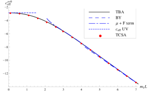
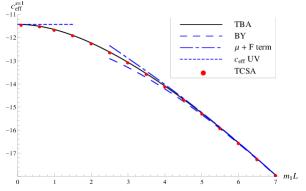
Figure 4.1: Effective central charge for the excited states with momentum quantum number $s=0,1$ from TBA and TCSA, with the UV (CFT value) and IR asymptotics ($\mu$ and F term).

The excited state TBA equations are solved numerically by simultaneously iterating eqns. (4.1.1) and (4.2) in large volume, where the asymptotic of the pole position (4.5) can be used as a starting point. Using this solution the volume is decreased and the equations iterated, and continuing this process the solution can be tracked to small volume. For $s\neq 0$ the numerics is straightforward to perform up to precision of order $10^{-12}$, and all the ingredients to calculate the conjecture (2.15) can be readily constructed. For $s=0$ there exists a critical volume $r_{c}$ under which it is necessary to be more careful with the numerical calculation.

4.1.2 Zero-momentum state: desingularization in small volume

As described in details in [41, 42, 43], for states containing a zero-momentum particle it can happen that under a given critical volume $r_{c}$ some singularity ends up being on the integration contour. To describe this situation, we recall that the $Y$-system (2.9) gives relations between positions where the functions $Y_{\alpha}=e^{\varepsilon_{\alpha}}$ take the values 0 and $-1$, which are the logarithmic singular points of the TBA equations. For the $T_{2}$ model the incidence matrix is given by

$$I^{\left[T_{2}\right]} = \begin{pmatrix}0&1\\ 1&1\end{pmatrix}\qquad\mbox{and}\qquad h=5$$ (4.10)

For the excited state containing a single type-1 particle with zero momentum in large volume there are active singularities on the imaginary axis at $\pm\bar{\theta}_{1}$ with

$$\bar{\theta}_{1}=i\frac{\pi}{10}+i\delta$$ (4.11)

with $\delta>0$ where $Y_{2}=-1$. From (2.9) it follows that $Y_{2}=-1$ at $\bar{\theta}_{1}-i\frac{2\pi}{5}$ and $-\bar{\theta}_{1}+i\frac{2\pi}{5}$, and $Y_{1}=Y_{2}=0$ at positions $\bar{\theta}_{1}-i\frac{\pi}{5}$ and $-\bar{\theta}_{1}+i\frac{\pi}{5}$. As the volume decreases, the value of $\delta$ increases till at some critical value of the volume given by $m_{1}L=r_{c}$ it reaches $\delta_{c}=\frac{\pi}{10}$. At this point $\bar{\theta}_{1}=-\bar{\theta}_{1}+i\frac{2\pi}{5}$ resulting in a coincidence of singularities, and also of zeros. Decreasing the volume to $m_{1}L<r_{c}$ results in the “scattering“ of the singularities on each other at right angles pushing them away from the imaginary axis with fixed imaginary part in the form

$$\bar{\theta}_{1}=i\frac{\pi}{5}+\alpha$$ (4.12)

As a result, the zeros of $Y_{1}$ and $Y_{2}$ sit exactly on the integration contour, making the equation for the pseudo-energy (4.1.1) singular and leading to instabilities in the numerical solution of the TBA equations.

One way to handle the numerical treatment of the problem is to shift the integration contour, while an alternative is to rearrange the self-consistent equations appropriately, which is called desingularization. The latter approach relies on the relation [43]

$$\varphi_{ad}\left(\theta\right) = -\varphi_{h}\left(\theta\right)I_{ad}^{\left[T_{2}\right]}+\sum_{b}\int\frac{\mathrm{d}\theta^{\prime}}{2\pi}\varphi_{ab}\left(\theta-\theta^{\prime}\right)\varphi_{h}\left(\theta^{\prime}\right)I_{bd}^{\left[T_{2}\right]}$$

$$\varphi_{h}\left(\theta\right) = \frac{h}{2\cosh\left(\frac{h}{2}\theta\right)}=\pm i\partial_{\theta}\log\left(\sigma_{h}\left(\theta\pm i\frac{\pi}{h}\right)\right)$$

$$\sigma_{h}\left(\theta\right) = \tanh\left(\frac{h}{4}\theta\right)$$ (4.13)

which allows the TBA equations to be recast as

$$\hat{\varepsilon}_{a}\left(\theta\right) = \varepsilon_{a}\left(\theta\right)-\log\left(\sigma\left(\theta^{\prime}-\tilde{\theta}_{1}\right)\sigma\left(\theta^{\prime}-\tilde{\theta}_{2}\right)\right)$$

$$\hat{\varepsilon}_{a}\left(\theta\right) = m_{a}L\cosh\left(\theta\right)-\sum_{b}\int\frac{\mathrm{d}\theta^{\prime}}{2\pi}\varphi_{ab}\left(\theta-\theta^{\prime}\right)\log\left(\sigma\left(\theta^{\prime}-\tilde{\theta}_{1}\right)\sigma\left(\theta^{\prime}-\tilde{\theta}_{2}\right)+e^{-\hat{\varepsilon}_{b}\left(\theta^{\prime}\right)}\right)$$

$$e^{\hat{\varepsilon}_{a}\left(\bar{\theta}_{1}\right)} = i\coth\left(\frac{5}{2}\tilde{\theta}_{1}+i\frac{\pi}{4}\right)$$

$$E_{\mathrm{TBA}}\left(L\right) = -\sum_{a}\int\frac{\mathrm{d}\theta}{2\pi}m_{a}\cosh\left(\theta\right)\log\left(\sigma\left(\theta-\tilde{\theta}_{1}\right)\sigma\left(\theta-\tilde{\theta}_{2}\right)+e^{-\hat{\varepsilon}_{b}\left(\theta\right)}\right)$$ (4.14)

where $\tilde{\theta}_{1}=\bar{\theta}_{1}-i\frac{\pi}{h}$, $\tilde{\theta}_{2}=\bar{\theta}_{2}+i\frac{\pi}{h}$. These equations are regular and can be iterated in a stable way, however, the available precision using double precision numbers drops to the order of $10^{-10}$. Fortunately, that is still more than sufficient for our purposes.

To calculate the densities and $\left\langle\Theta\right\rangle$ under $r_{c}$ we need to desingularize $f_{s},f_{c},f_{i}$ in (3.4) as well. It’s easy to see, that the equation for $f_{s}$ and $f_{c}$ is regular under $r_{c}$ , since $\frac{1}{1+e^{\varepsilon_{\alpha}}}$ at the singularity position is regular, because $Y_{\alpha}=e^{\varepsilon_{\alpha}}=0$. For $f_{i}$ the source term $\varphi$ is singular at $\tilde{\theta}_{1,2}$, hence it is necessary to desingularize it:

$$\hat{f}_{i,\alpha}\left(\theta\right) = f_{i,\alpha}\left(\theta\right)+\varphi_{h}\left(\theta-\bar{\theta}_{i}\right)$$

$$\hat{f}_{i,\alpha}\left(\theta\right) = \sum_{\beta}\int\frac{\mathrm{d}\theta^{\prime}}{2\pi}\varphi_{\alpha\beta}\left(\theta-\theta^{\prime}\right)\frac{e^{\varepsilon_{\beta}\left(\theta^{\prime}\right)}\varphi_{h}\left(\theta-\bar{\theta}_{i}\right)+\hat{f}_{i,\beta}\left(\theta^{\prime}\right)}{1+e^{\varepsilon_{\beta}\left(\theta^{\prime}\right)}}$$ (4.15)

For numerical calculations the form

$$\hat{f}_{1,\alpha}\left(\theta\right) = \sum_{\beta}\int\frac{\mathrm{d}\theta^{\prime}}{2\pi}\varphi_{\alpha\beta}\left(\theta-\theta^{\prime}\right)\frac{\partial\sigma\left(\theta^{\prime}-\tilde{\theta}_{1}\right)\sigma\left(\theta^{\prime}-\tilde{\theta}_{2}\right)+e^{-\hat{\varepsilon}_{b}\left(\theta^{\prime}\right)}\hat{f}_{1,\beta}\left(\theta^{\prime}\right)}{\sigma\left(\theta^{\prime}-\tilde{\theta}_{1}\right)\sigma\left(\theta^{\prime}-\tilde{\theta}_{2}\right)+e^{-\hat{\varepsilon}_{b}\left(\theta^{\prime}\right)}}$$

$$\hat{f}_{2,\alpha}\left(\theta\right) = \sum_{\beta}\int\frac{\mathrm{d}\theta^{\prime}}{2\pi}\varphi_{\alpha\beta}\left(\theta-\theta^{\prime}\right)\frac{\sigma\left(\theta^{\prime}-\tilde{\theta}_{1}\right)\partial\sigma\left(\theta^{\prime}-\tilde{\theta}_{2}\right)+e^{-\hat{\varepsilon}_{b}\left(\theta^{\prime}\right)}\hat{f}_{1,\beta}\left(\theta^{\prime}\right)}{\sigma\left(\theta^{\prime}-\tilde{\theta}_{1}\right)\sigma\left(\theta^{\prime}-\tilde{\theta}_{2}\right)+e^{-\hat{\varepsilon}_{b}\left(\theta^{\prime}\right)}}$$ (4.16)

is more convenient.

4.2 Densities and the conjecture for states with a single type-1 particle

The derivatives of the quantization condition can be written like (3.11) with the help of the definitions in (3.4), (3.12) for the single type-1 state

$$\frac{\partial\left(Q_{1},Q_{2}\right)}{\partial\left(\bar{\theta}_{1},\bar{\theta}_{2}\right)} = \left(\begin{array}[]{cc}L\mathcal{N}_{1}+\mathcal{N}_{\varphi}&-\mathcal{N}_{\varphi}\\ -\mathcal{N}_{\varphi}&L\mathcal{N}_{2}+\mathcal{N}_{\varphi}\end{array}\right)$$ (4.19)

where

$$\mathcal{N}_{1} = -if_{s,2}\left(\bar{\theta}_{1}\right)=-im_{2}\sinh\left(\bar{\theta}_{1}\right)-i\sum_{\beta}\int\frac{\mathrm{d}\theta^{\prime}}{2\pi}\varphi_{2\beta}\left(\bar{\theta}_{1}-\theta^{\prime}\right)\frac{f_{s,\beta}\left(\theta^{\prime}\right)}{1+e^{\varepsilon_{\beta}\left(\theta^{\prime}\right)}}$$

$$\mathcal{N}_{2} = if_{s,2}\left(\bar{\theta}_{2}\right)=im_{2}\sinh\left(\bar{\theta}_{2}\right)+i\sum_{\beta}\int\frac{\mathrm{d}\theta^{\prime}}{2\pi}\varphi_{2\beta}\left(\bar{\theta}_{2}-\theta^{\prime}\right)\frac{f_{s,\beta}\left(\theta^{\prime}\right)}{1+e^{\varepsilon_{\beta}\left(\theta^{\prime}\right)}}$$

$$\mathcal{N}_{\varphi} = -f_{2,2}\left(\bar{\theta}_{1}\right)=-\varphi_{22}\left(\bar{\theta}_{1}-\bar{\theta}_{2}\right)-\sum_{\beta}\int\frac{\mathrm{d}\theta^{\prime}}{2\pi}\varphi_{2\beta}\left(\bar{\theta}_{1}-\theta^{\prime}\right)\frac{f_{2,\beta}\left(\theta^{\prime}\right)}{1+e^{\varepsilon_{\beta}\left(\theta^{\prime}\right)}}$$ (4.20)

$$= -f_{1,2}\left(\bar{\theta}_{2}\right)=-\varphi_{22}\left(\bar{\theta}_{2}-\bar{\theta}_{1}\right)-\sum_{\beta}\int\frac{\mathrm{d}\theta^{\prime}}{2\pi}\varphi_{2\beta}\left(\bar{\theta}_{2}-\theta^{\prime}\right)\frac{f_{1,\beta}\left(\theta^{\prime}\right)}{1+e^{\varepsilon_{\beta}\left(\theta^{\prime}\right)}}$$

For the case $s=0$ and $m_{1}L<r_{c}$

$$\mathcal{N}_{\varphi} = -\hat{f}_{2,2}\left(\bar{\theta}_{1}\right)+\varphi_{h}\left(\bar{\theta}_{1}-\bar{\theta}_{2}\right)=+\varphi_{h}\left(\bar{\theta}_{1}-\bar{\theta}_{2}\right)$$ (4.21)

$$-\sum_{\beta}\int\frac{\mathrm{d}\theta^{\prime}}{2\pi}\varphi_{\alpha\beta}\left(\bar{\theta}_{1}-\theta^{\prime}\right)\frac{\sigma\left(\theta^{\prime}-\tilde{\theta}_{1}\right)\partial\sigma\left(\theta^{\prime}-\tilde{\theta}_{2}\right)+e^{-\hat{\varepsilon}_{b}\left(\theta^{\prime}\right)}\hat{f}_{1,\beta}\left(\theta^{\prime}\right)}{\sigma\left(\theta^{\prime}-\tilde{\theta}_{1}\right)\sigma\left(\theta^{\prime}-\tilde{\theta}_{2}\right)+e^{-\hat{\varepsilon}_{b}\left(\theta^{\prime}\right)}}$$

$$= -\hat{f}_{1,2}\left(\bar{\theta}_{2}\right)+\varphi_{h}\left(\bar{\theta}_{2}-\bar{\theta}_{1}\right)=+\varphi_{h}\left(\bar{\theta}_{2}-\bar{\theta}_{1}\right)$$

$$-\sum_{\beta}\int\frac{\mathrm{d}\theta^{\prime}}{2\pi}\varphi_{\alpha\beta}\left(\bar{\theta}_{2}-\theta^{\prime}\right)\frac{\partial\sigma\left(\theta^{\prime}-\tilde{\theta}_{1}\right)\sigma\left(\theta^{\prime}-\tilde{\theta}_{2}\right)+e^{-\hat{\varepsilon}_{b}\left(\theta^{\prime}\right)}\hat{f}_{1,\beta}\left(\theta^{\prime}\right)}{\sigma\left(\theta^{\prime}-\tilde{\theta}_{1}\right)\sigma\left(\theta^{\prime}-\tilde{\theta}_{2}\right)+e^{-\hat{\varepsilon}_{b}\left(\theta^{\prime}\right)}}$$

With the above densities the conjecture for the form factor series (2.15) for this state takes the form

$$\left\langle\bar{\theta}_{1},\bar{\theta}_{2}\right|\mathcal{O}\left|\bar{\theta}_{1},\bar{\theta}_{2}\right\rangle_{L} = \sum_{n_{1},n_{2}=0}^{\infty}\frac{1}{n_{1}!n_{2}!}\int_{-\infty}^{\infty}\prod_{j=1}^{\tilde{N}}\frac{\mathrm{d}\theta_{j}}{2\pi\left[1+e^{\varepsilon_{\alpha_{j}}\left(\theta_{j}\right)}\right]}\Biggl{[}$$ (4.22)

$$F_{2n_{1},2n_{2},c}^{\mathcal{O}}\left(\theta_{1},\dots,\theta_{\tilde{N}}\right)+\frac{1}{L^{2}\mathcal{N}_{1}\mathcal{N}_{2}+\mathcal{N}_{\varphi}L\left(\mathcal{N}_{1}+\mathcal{N}_{2}\right)}\Biggl{\{}$$

$$+\left(L\mathcal{N}_{1}+\mathcal{N}_{\varphi}\right)F_{2n_{1},2n_{2}+2,c}^{\mathcal{O}}\left(\bar{\theta}_{1},\theta_{1},\dots,\theta_{\tilde{N}}\right)$$

$$+\left(L\mathcal{N}_{2}+\mathcal{N}_{\varphi}\right)F_{2n_{1},2n_{2}+2,c}^{\mathcal{O}}\left(\bar{\theta}_{2},\theta_{1},\dots,\theta_{\tilde{N}}\right)$$

$$+F_{2n_{1},2n_{2}+4,c}^{\mathcal{O}}\left(\bar{\theta}_{1},\bar{\theta}_{2},\theta_{1},\dots,\theta_{\tilde{N}}\right)\Biggr{\}}\Biggr{]}$$

5 Numerical results

The last ingredient needed to compute the form factor series (2.15) is the numerical evaluation of the connected diagonal form factors of the $T_{2}$ model. This is rather nontrivial to perform in a sufficiently quick and numerically stable way for large number of particles. Since this is a task that is also important for evaluating the spectral series for correlation functions at finite temperature [20, 23, 24, 61], we describe the required tricks in Appendix A. The procedure can be straightforwardly generalized to connected diagonal form factors in other integrable models.

In large volume a rough estimate for the magnitude of the terms in the series comes from the behaviour of the filling fractions

$$\prod_{i}\frac{1}{1+e^{\varepsilon_{\alpha_{j}}\left(\theta_{j}\right)}}\lesssim e^{-\left(\sum_{i}m_{i}\right)L}$$

where $m_{i}$ are the masses of the particles contained in the given state. Using this estimate we can identify the terms of the series that give the dominant contribution to the expectation value. However, with decreasing volume the ordering of the terms can change depending on the behaviour of the pseudo-energy functions; in addition, to maintain accuracy it is necessary to add progressively more terms. As a result, the form factor series (2.15) is effectively an infrared (low energy/large volume) expansion for the expectation value.

For our numerical calculations we implemented the terms with less than 4 integrals, since for higher terms the number of integrals and the size of the form factors makes the numerical integration too time-consuming; in addition, the terms incorporated already show an excellent agreement with the conjecture. Table 5.1 shows the terms calculated for numerics.

$\begin{array}[t]{|c||c|c|c|c|c|c|c|c|}\hline\cr\mbox{label}&0&1&2&11&12&111&22&112\\ \hline\cr\hline\cr\mbox{\#\,\ of\,\ type-1\,\ integrals}&0&1&0&2&1&3&0&2\\ \hline\cr\mbox{\#\,\ of\,\ type-2\,\ integrals}&0&0&1&0&1&0&2&1\\ \hline\cr\mbox{magnitude/L}&0&m_{1}&m_{2}&2m_{1}&m_{1}+m_{2}&3m_{1}&2m_{2}&2m_{1}+m_{2}\\ \hline\cr\end{array}$

Table 5.1: The terms incorporated from the form factor series into the numerical calculation.

In the $T_{2}$ model there are two primary operators, namely $\Phi_{1,3}$ and $\Phi_{1,2}$. $\Phi_{1,3}$ is the operator perturbing the UV limit of the model, hence it’s proportional to $\Theta$

$$\Theta = 2\pi\lambda\left(2h_{1,3}-2\right)\Phi_{1,3}$$ (5.1)

where $h_{1,3}$ is the conformal weight of the $\Phi_{1,3}$ and $\lambda$ is the coupling constant of the perturbation that is proportional to the mass gap [62]

$$\lambda = \kappa m_{1}^{2-2h_{1,3}}$$ (5.2)

with

$$\kappa = \text{\textminus}0.04053795542...$$ (5.3)

Because of this, the form factor series for $\Phi_{1,3}$ is equivalent to the TBA equation as proved in Section 3, and the numerical calculation for $\Phi_{1,3}$ is therefore not a real further test for the general validity of the form factor series (2.15). However it is still useful since with its expectation value known from TBA equations one can get an independent check of the numerical precision of TCSA, and the convergence of the form factor series. For $\Phi_{1,2}$ there is only TCSA and the form factor series, with the numerical deviation for $\Phi_{1,3}$ setting the expected precision for the agreement between them.

For the numerical integration we used the Cuba library routines [63], called from inside Wolfram Mathematica [64].

5.1 Moving one-particle state, $s=1$

For the moving type-1 excited state with momentum quantum number $s=1$, Figure 5.1 shows the expectation value $\!{}_{1}\left\langle\left\{1\right\}\right|\Phi_{1,3}\left|\left\{1\right\}\right\rangle_{1}$ calculated with RG-extrapolated TCSA, from TBA together with the results from the form factor series (4.22) obtained by adding progressively more terms. The precision of the TBA is of the order $10^{-12}$ and comparing it with the TCSA data, we find that the precision of the RG-extrapolated TCSA is of order $10^{-6}-10^{-7}$. Table 5.2 shows the difference between the form factor series with different terms involved and the TCSA data. For volume $m_{1}L>5$ the difference between the form factor series up to and including the $112$ term, and the TCSA is in the order of the TCSA error, and including more terms make the agreement better for smaller volume as well.

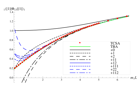
Figure 5.1: $\!{}_{1}\!\!\left\langle\left\{1\right\}\right|\Phi_{1,3}\left|\left\{1\right\}\right\rangle_{1}$ evaluated by the form factor series including different contributions, RG extrapolated TCSA and TBA. Here and in all subsequent plots matrix elements are given in units of $m_{1}$.

For $\Phi_{1,2}$ the results for the quantity $i\!_{1}\!\!\left\langle\left\{1\right\}\right|\Phi_{1,2}\left|\left\{1\right\}\right\rangle_{1}$ are shown in Figure 5.2, and the difference between the form factor series and the TCSA is given in Table 5.3. We note that since from (A.14) it follows that the matrix elements of $\Phi_{1,2}$ are imaginary, here and in all subsequent figures and tables concerning $\Phi_{1,2}$ we multiply all data by $i$. The form factor series shows excellent agreement with the TCSA for volume $m_{1}L>5$, and again including more terms the agreement is better for smaller volumes. As noted before, the correctness of the form factor series does not follow from TBA, hence this is a nontrivial verification of the form factor series.

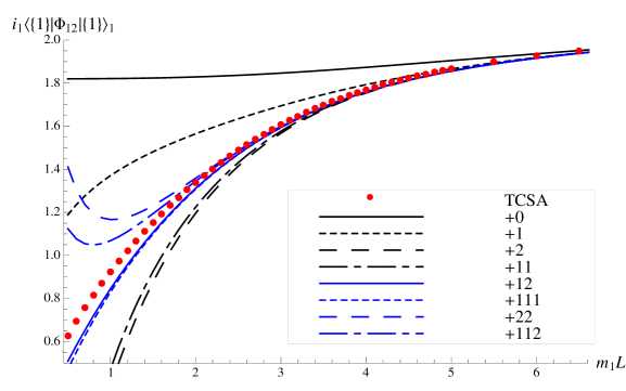
Figure 5.2: $i\,_{1}\!\!\left\langle\left\{1\right\}\right|\Phi_{1,2}\left|\left\{1\right\}\right\rangle_{1}$ evaluated by the form factor series including different contributions and RG-extrapolated TCSA.

$\begin{array}[]{|c||c|c|c|c|c|c|c|c|}\hline\cr m_{1}L&0&+1&+2&+11&+12&+111&+22&+112\\ \hline\cr\hline\cr 0.5&-0.8115&-1\cdot 10^{-2}&1.039&0.7047&-0.3024&-0.1995&-0.8307&-0.3166\\ \hline\cr 1&-0.6554&-0.1143&0.5094&0.3528&-7\cdot 10^{-2}&-4\cdot 10^{-2}&-0.2652&-0.1089\\ \hline\cr 1.5&-0.5173&-0.1256&0.2649&0.1813&-2\cdot 10^{-2}&-2\cdot 10^{-3}&-9\cdot 10^{-2}&-4\cdot 10^{-2}\\ \hline\cr 2&-0.3966&-0.1079&0.1362&9\cdot 10^{-2}&-2\cdot 10^{-3}&4\cdot 10^{-3}&-3\cdot 10^{-2}&-1\cdot 10^{-2}\\ \hline\cr 2.5&-0.2947&-8\cdot 10^{-2}&7\cdot 10^{-2}&4\cdot 10^{-2}&5\cdot 10^{-4}&3\cdot 10^{-3}&-1\cdot 10^{-2}&-4\cdot 10^{-3}\\ \hline\cr 3&-0.2124&-6\cdot 10^{-2}&3\cdot 10^{-2}&2\cdot 10^{-2}&6\cdot 10^{-4}&2\cdot 10^{-3}&-3\cdot 10^{-3}&-1\cdot 10^{-3}\\ \hline\cr 3.5&-0.1489&-4\cdot 10^{-2}&1\cdot 10^{-2}&8\cdot 10^{-3}&3\cdot 10^{-4}&6\cdot 10^{-4}&-9\cdot 10^{-4}&-3\cdot 10^{-4}\\ \hline\cr 4&-0.102&-2\cdot 10^{-2}&6\cdot 10^{-3}&3\cdot 10^{-3}&1\cdot 10^{-4}&2\cdot 10^{-4}&-2\cdot 10^{-4}&-5\cdot 10^{-5}\\ \hline\cr 4.5&-7\cdot 10^{-2}&-1\cdot 10^{-2}&3\cdot 10^{-3}&1\cdot 10^{-3}&4\cdot 10^{-5}&8\cdot 10^{-5}&-5\cdot 10^{-5}&-1\cdot 10^{-5}\\ \hline\cr 5&-5\cdot 10^{-2}&-7\cdot 10^{-3}&1\cdot 10^{-3}&4\cdot 10^{-4}&1\cdot 10^{-5}&2\cdot 10^{-5}&-1\cdot 10^{-5}&-2\cdot 10^{-6}\\ \hline\cr 5.5&-3\cdot 10^{-2}&-4\cdot 10^{-3}&5\cdot 10^{-4}&1\cdot 10^{-4}&4\cdot 10^{-6}&7\cdot 10^{-6}&-3\cdot 10^{-6}&-4\cdot 10^{-7}\\ \hline\cr 6&-2\cdot 10^{-2}&-2\cdot 10^{-3}&2\cdot 10^{-4}&4\cdot 10^{-5}&8\cdot 10^{-7}&2\cdot 10^{-6}&-7\cdot 10^{-7}&-2\cdot 10^{-7}\\ \hline\cr 6.5&-1\cdot 10^{-2}&-1\cdot 10^{-3}&7\cdot 10^{-5}&1\cdot 10^{-5}&4\cdot 10^{-7}&6\cdot 10^{-7}&3\cdot 10^{-8}&1\cdot 10^{-7}\\ \hline\cr 7&-8\cdot 10^{-3}&-5\cdot 10^{-4}&3\cdot 10^{-5}&5\cdot 10^{-6}&4\cdot 10^{-7}&4\cdot 10^{-7}&3\cdot 10^{-7}&3\cdot 10^{-7}\\ \hline\cr\end{array}$

Table 5.2: The difference between the evaluations of $\!{}_{1}\!\!\left\langle\left\{1\right\}\right|\Phi_{1,3}\left|\left\{1\right\}\right\rangle_{1}$ from the RG-extrapolated TCSA and the form factor series, depending on the multi-particle contributions included in the latter.

$\begin{array}[]{|c||c|c|c|c|c|c|c|c|}\hline\cr m_{1}L&0&+1&+2&+11&+12&+111&+22&+112\\ \hline\cr\hline\cr 0.5&-1.203&-0.5712&1.113&0.9523&0.1086&0.1457&-0.7935&-0.5066\\ \hline\cr 1&-0.9067&-0.4563&0.5275&0.4431&7\cdot 10^{-2}&8\cdot 10^{-2}&-0.252&-0.1539\\ \hline\cr 1.5&-0.6803&-0.3379&0.2661&0.2171&4\cdot 10^{-2}&4\cdot 10^{-2}&-9\cdot 10^{-2}&-5\cdot 10^{-2}\\ \hline\cr 2&-0.5&-0.2361&0.1325&0.1038&2\cdot 10^{-2}&2\cdot 10^{-2}&-3\cdot 10^{-2}&-2\cdot 10^{-2}\\ \hline\cr 2.5&-0.3581&-0.1561&6\cdot 10^{-2}&5\cdot 10^{-2}&7\cdot 10^{-3}&9\cdot 10^{-3}&-9\cdot 10^{-3}&-5\cdot 10^{-3}\\ \hline\cr 3&-0.2498&-1\cdot 10^{-1}&3\cdot 10^{-2}&2\cdot 10^{-2}&3\cdot 10^{-3}&3\cdot 10^{-3}&-3\cdot 10^{-3}&-1\cdot 10^{-3}\\ \hline\cr 3.5&-0.1701&-6\cdot 10^{-2}&1\cdot 10^{-2}&8\cdot 10^{-3}&1\cdot 10^{-3}&1\cdot 10^{-3}&-8\cdot 10^{-4}&-3\cdot 10^{-4}\\ \hline\cr 4&-0.1136&-3\cdot 10^{-2}&5\cdot 10^{-3}&3\cdot 10^{-3}&3\cdot 10^{-4}&4\cdot 10^{-4}&-2\cdot 10^{-4}&-6\cdot 10^{-5}\\ \hline\cr 4.5&-7\cdot 10^{-2}&-2\cdot 10^{-2}&2\cdot 10^{-3}&1\cdot 10^{-3}&9\cdot 10^{-5}&1\cdot 10^{-4}&-5\cdot 10^{-5}&-1\cdot 10^{-5}\\ \hline\cr 5&-5\cdot 10^{-2}&-1\cdot 10^{-2}&9\cdot 10^{-4}&4\cdot 10^{-4}&3\cdot 10^{-5}&3\cdot 10^{-5}&-1\cdot 10^{-5}&-3\cdot 10^{-6}\\ \hline\cr 5.5&-3\cdot 10^{-2}&-5\cdot 10^{-3}&4\cdot 10^{-4}&1\cdot 10^{-4}&6\cdot 10^{-6}&8\cdot 10^{-6}&-3\cdot 10^{-6}&-2\cdot 10^{-6}\\ \hline\cr 6&-2\cdot 10^{-2}&-3\cdot 10^{-3}&1\cdot 10^{-4}&4\cdot 10^{-5}&2\cdot 10^{-7}&8\cdot 10^{-7}&-2\cdot 10^{-6}&-2\cdot 10^{-6}\\ \hline\cr 6.5&-1\cdot 10^{-2}&-1\cdot 10^{-3}&5\cdot 10^{-5}&1\cdot 10^{-5}&-1\cdot 10^{-6}&-1\cdot 10^{-6}&-2\cdot 10^{-6}&-2\cdot 10^{-6}\\ \hline\cr 7&-8\cdot 10^{-3}&-6\cdot 10^{-4}&2\cdot 10^{-5}&2\cdot 10^{-6}&-2\cdot 10^{-6}&-2\cdot 10^{-6}&-2\cdot 10^{-6}&-2\cdot 10^{-6}\\ \hline\cr\end{array}$

Table 5.3: The difference between the evaluations of $i\,_{1}\!\!\left\langle\left\{1\right\}\right|\Phi_{1,2}\left|\left\{1\right\}\right\rangle_{1}$ from the RG-extrapolated TCSA and the form factor series, depending on the multi-particle contributions included in the latter.

5.2 Zero-momentum one-particle state, $s=0$

As seen for the $s=1$ case the form factor series reproduce the expectation value of local operators with very good precision in large volume, even by including only few terms from the series. The expectation is that for any state in small volume it is necessary to include higher contributions of the series, but for any desired accuracy a finite number of them is sufficient.

As shown below, this expectation is challenged by the nontrivial transition in the TBA equation for standing state at $r_{c}$. Figure 5.3 and 5.4 shows the result for the expectation values of $\Phi_{1,3}$ and $\Phi_{1,2}$, while Table 5.4 and 5.5 list the numerical deviations from RG-extrapolated TCSA.

For large volume ($m_{1}L\gtrsim 6$) the agreement between the form factor series and the TCSA is again excellent. However, towards the critical volume $\left(r_{c}\sim 2.66\right)$ the terms of the form factor series tend to diverge. This can be understood from the fact that the total density of the states

$$\rho_{tot}=\det\mathcal{K}=L^{2}\mathcal{N}_{1}\mathcal{N}_{2}+\mathcal{N}_{\varphi}L\left(\mathcal{N}_{1}+\mathcal{N}_{2}\right)$$ (5.4)

which the denominator of the form factor series (4.22), is zero at $r_{c}$. Figure 5.5 shows the behaviour of $\rho_{tot}$ around $r_{c}$; fitting the location where $\rho_{tot}\left(\tilde{r}_{c}\right)=0$, the result is

$$\tilde{r}_{c}=2.6646510318$$ (5.5)

which is perfect agreement with the value of $r_{c}$ obtained in [43].

The reason for $\rho_{tot}$ vanishing at $r_{c}$ can be understood from the excited TBA. Since the active singularities coincide at this point, the density which is the Jacobi determinant of the quantization condition for the active singularities, is zero due to the degeneracy. Such singularities of the density were observed previously for the finite volume form factors formula in [45]; however in that case including the exponential corrections resolved (or at least shifted) the singularity. The present situation is different as all exponential corrections to the density are already included. To resolve the singularity it would be necessary to include every term of the form factor series, to compensate the zero of the denominator.

This conclusion is also supported by the behaviour of the pseudo-energies and the filling fractions around $r_{c}$. Approaching $r_{c}$ the filling fractions no more suppress the higher order terms in the series and the ordering of terms by their magnitude is not valid anymore, i.e. every terms is important in the series. This is consistent with the procedure of desingularization, whereby to describe the excited state level with the TBA equation under $r_{c}$ it was necessary to redefine the pseudo-energy to have a form which is finite and convergent under iterations.

For the form factor series a similar rearrangement is necessary close to and under $r_{c}$. Unfortunately such a rearrangement is not yet known, and this sets the practical validity of the form factor series to IR regions where no nontrivial transitions occur in the TBA equations.

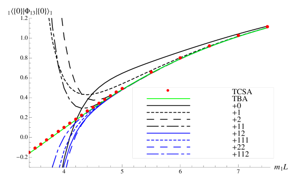
Figure 5.3: $\!{}_{1}\!\!\left\langle\left\{0\right\}\right|\Phi_{1,3}\left|\left\{0\right\}\right\rangle_{1}$ calculated by the form factor series including different contributions, RG extrapolated TCSA and TBA.

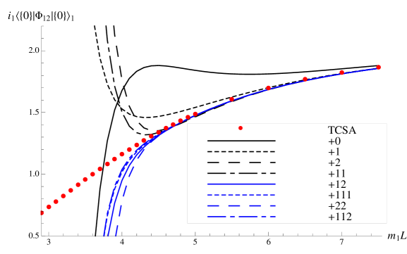
Figure 5.4: $i\,_{1}\!\!\left\langle\left\{0\right\}\right|\Phi_{1,2}\left|\left\{0\right\}\right\rangle_{1}$ calculated by the form factor series including different contributions and RG extrapolated TCSA.

$\begin{array}[]{|c||c|c|c|c|c|c|c|c|}\hline\cr m_{1}L&0&+1&+2&+11&+12&+111&+22&+112\\ \hline\cr\hline\cr 4&0.3114&-0.4977&-0.9218&-0.4061&0.3695&0.2265&0.494&9\cdot 10^{-2}\\ \hline\cr 4.5&-0.1529&-0.1416&-8\cdot 10^{-2}&-2\cdot 10^{-2}&3\cdot 10^{-2}&2\cdot 10^{-2}&3\cdot 10^{-2}&3\cdot 10^{-3}\\ \hline\cr 5&-0.1637&-6\cdot 10^{-2}&9\cdot 10^{-4}&5\cdot 10^{-3}&3\cdot 10^{-3}&2\cdot 10^{-3}&1\cdot 10^{-3}&-3\cdot 10^{-5}\\ \hline\cr 5.5&-0.114&-3\cdot 10^{-2}&4\cdot 10^{-3}&2\cdot 10^{-3}&3\cdot 10^{-4}&3\cdot 10^{-4}&-4\cdot 10^{-5}&-3\cdot 10^{-5}\\ \hline\cr 6&-7\cdot 10^{-2}&-1\cdot 10^{-2}&2\cdot 10^{-3}&8\cdot 10^{-4}&5\cdot 10^{-5}&5\cdot 10^{-5}&-2\cdot 10^{-5}&-5\cdot 10^{-6}\\ \hline\cr 6.5&-4\cdot 10^{-2}&-6\cdot 10^{-3}&7\cdot 10^{-4}&2\cdot 10^{-4}&7\cdot 10^{-6}&1\cdot 10^{-5}&-5\cdot 10^{-6}&-9\cdot 10^{-7}\\ \hline\cr 7&-3\cdot 10^{-2}&-3\cdot 10^{-3}&2\cdot 10^{-4}&6\cdot 10^{-5}&1\cdot 10^{-6}&2\cdot 10^{-6}&-1\cdot 10^{-6}&-4\cdot 10^{-7}\\ \hline\cr 7.5&-2\cdot 10^{-2}&-1\cdot 10^{-3}&8\cdot 10^{-5}&2\cdot 10^{-5}&1\cdot 10^{-7}&4\cdot 10^{-7}&-2\cdot 10^{-7}&-1\cdot 10^{-7}\\ \hline\cr\end{array}$

Table 5.4: The difference between the evaluatons of $\!{}_{1}\!\!\left\langle\left\{0\right\}\right|\Phi_{1,3}\left|\left\{0\right\}\right\rangle_{1}$ from the RG-extrapolated TCSA and the form factor series, depending on the multi-particle contributions included in the latter.

$\begin{array}[]{|c||c|c|c|c|c|c|c|c|}\hline\cr m_{1}L&0&+1&+2&+11&+12&+111&+22&+112\\ \hline\cr\hline\cr 4&-0.5274&-0.3774&-0.6113&-0.3511&0.2018&0.1321&0.3664&0.1129\\ \hline\cr 4.5&-0.5513&-0.139&-2\cdot 10^{-2}&-9\cdot 10^{-3}&2\cdot 10^{-2}&1\cdot 10^{-2}&2\cdot 10^{-2}&4\cdot 10^{-3}\\ \hline\cr 5&-0.3645&-6\cdot 10^{-2}&1\cdot 10^{-2}&7\cdot 10^{-3}&1\cdot 10^{-3}&1\cdot 10^{-3}&3\cdot 10^{-4}&4\cdot 10^{-6}\\ \hline\cr 5.5&-0.2176&-3\cdot 10^{-2}&7\cdot 10^{-3}&3\cdot 10^{-3}&2\cdot 10^{-4}&2\cdot 10^{-4}&-1\cdot 10^{-4}&-3\cdot 10^{-5}\\ \hline\cr 6&-0.1255&-1\cdot 10^{-2}&3\cdot 10^{-3}&9\cdot 10^{-4}&3\cdot 10^{-5}&5\cdot 10^{-5}&-3\cdot 10^{-5}&-5\cdot 10^{-6}\\ \hline\cr 6.5&-7\cdot 10^{-2}&-7\cdot 10^{-3}&9\cdot 10^{-4}&2\cdot 10^{-4}&5\cdot 10^{-6}&1\cdot 10^{-5}&-6\cdot 10^{-6}&-2\cdot 10^{-6}\\ \hline\cr 7&-4\cdot 10^{-2}&-3\cdot 10^{-3}&3\cdot 10^{-4}&6\cdot 10^{-5}&-2\cdot 10^{-7}&1\cdot 10^{-6}&-2\cdot 10^{-6}&-1\cdot 10^{-6}\\ \hline\cr 7.5&-2\cdot 10^{-2}&-1\cdot 10^{-3}&9\cdot 10^{-5}&1\cdot 10^{-5}&-1\cdot 10^{-6}&-1\cdot 10^{-6}&-2\cdot 10^{-6}&-2\cdot 10^{-6}\\ \hline\cr\end{array}$

Table 5.5: The difference between the evaluations of $i\,_{1}\!\!\left\langle\left\{0\right\}\right|\Phi_{1,2}\left|\left\{0\right\}\right\rangle_{1}$ from the RG-extrapolated TCSA and the form factor series, depending on the multi-particle contributions included in the latter.

Figure 5.5: $\rho_{tot}$ for s=0

6 Conclusions and outlook

In this paper we presented a conjecture for the finite volume excited state expectation values of local operators in integrable quantum field theories. This conjecture is an extension of an earlier one [39] to models with a non-trivial bootstrap structure. The conjecture was supported by a combination of analytic and numerical evidence.

An important aspect of our result is that it gives the full specification of the $\mu$-terms from the excited state TBA. In the previous approach [35, 36], the determination of these terms was ambiguous due to the fact that in many cases a particle could be represented in several ways as bound state of others. The series (2.15) specifies the $\mu$-term as the one corresponding to the way the particle is composed in terms of the singularities entering the excited state TBA equations, which provides a solution for the case of integrable models where the excited state TBA system is known. In addition, the series is exact, at least for values of the volume where it is convergent.

Unfortunately, for certain excited states this does not cover the whole volume range, as the TBA singularity configuration undergoes some rearrangement below some critical value of the volume. In the series (2.15) this is manifested in a singular behaviour of the terms, which prevent the extension of the series below the critical volume. Note that for the trace of the stress-energy tensor, the desingularized excited TBA gives such an extension. However, it is presently unclear how to implement the desingularization procedure directly for the series (2.15), so the description cannot be extended to other operators. In order to achieve that, one needs to separate the singularly behaved contributions and re-sum them to all orders, which is not an obvious task.

In this context we remark that based on the available studies of excited state TBA systems, the problematic rearrangement is only expected to happen for excited states for which some singularities are “stuck in the middle”, as opposed to going to the left/right asymptotic regions logarithmically with decreasing volume. Therefore, for most states the conjecture is expected to be valid for any value of the volume; obviously the smaller is the volume, the larger is the number of terms needed for a given precision. For states with a non-trivial transition in their singularity structure, the conjecture in its present form is expected to be valid for values of the volume above the critical one.

Another interesting issue is to extend the series to theories with non-diagonal scattering, starting with the series introduced in [61]. The formalism of finite volume form factors has been partially extended to these theories [65, 66]; unfortunately, it is exactly the general form of diagonal matrix elements that is at present not known in full generality.

Furthermore, the form of the terms in the series (2.15) is very suggestive for an extension to non-diagonal finite volume matrix elements; however, finding the precise form of such an extension is still an open question.

Finally, establishing the relation between the present framework, and the approaches based on separation of variables [14, 15] or fermionic structures [16, 17, 18] would be of interest, as it could lead to more efficient construction of finite size matrix elements and a deeper understanding of the underlying principles.

Acknowledgments

IMSZ is grateful to Roberto Tateo for the help with excited state TBA numerics and his hospitality in Turin, and also to the INFN and Campus Hungary Scholarship for financial support of the visit. IMSZ was also supported by funding from the People Programme (Marie Curie Actions) of the European Union’s Seventh Framework Programme FP7/2007-2013/ under REA Grant Agreement No 317089 (GATIS). BP and GT were supported by the Momentum grant LP2012-50/2014 of the Hungarian Academy of Sciences.

Appendix A Evaluation of connected diagonal form factors

Here we present a fast and efficient way to evaluate the connected diagonal form factors (defined in Section 2), which proceeds via the so-called symmetric form factors.

A.1 Form factors of the $T_{2}$ model

The form factors of primary fields in the $T_{2}$ model were constructed in [67]. For states containing only type-$1$ particles they are the same as form factors of certain exponential operators in the sinh-Gordon model with a specific value for the coupling constant. The form factors of the exponential operator

$$e^{kg\Phi}$$ (A.1)

in the sinh-Gordon model

$$\mathcal{L}=\frac{1}{2}\partial_{\mu}\Phi\partial^{\mu}\Phi-\lambda\cosh g\Phi$$ (A.2)

have the following form [68]

$$F_{n}^{(k)}\left(\theta_{1},\dots,\theta_{n}\right)=H_{n}\left[k\right]Q_{n}\left(x_{1},\dots,x_{n}\right)\prod_{i<j}\frac{F_{min}\left(\theta_{ij}\right)}{x_{i}+x_{j}}$$ (A.3)

where

$$\left[n\right]=\frac{\sin n\pi\frac{B}{2}}{\sin\pi\frac{B}{2}}\qquad B=\frac{2g^{2}}{8\pi+g^{2}}$$ (A.4)

and the minimal two-particle form factor is

$$F_{min}\left(\theta,B\right) = \mathcal{N}\exp\left[8\int_{0}^{\infty}\frac{\mathrm{d}x}{x}\frac{\sinh\frac{xB}{4}\sinh\frac{x}{2}\left(1-\frac{B}{2}\right)\sinh\frac{x}{2}}{\sinh^{2}x}\sin^{2}\left[\frac{x(i\pi-\theta)}{2\pi}\right]\right]$$

$$= \mathcal{N}\,e^{I(\theta,B)}$$

$$\mathcal{N} = \exp\left[-4\int\frac{\mathrm{d}x}{x}\frac{\sinh\frac{xB}{4}\sinh\frac{x}{2}\left(1-\frac{B}{2}\right)\sinh\frac{x}{2}}{\sinh^{2}x}\right]$$ (A.5)

with

$$I\left(\theta,B\right) = 8\int_{0}^{\infty}\frac{\mathrm{d}x}{x}\frac{\sinh\frac{xB}{4}\sinh\frac{x}{2}\left(1-\frac{B}{2}\right)\sinh\frac{x}{2}}{\sinh^{2}x}\sin^{2}\left[\frac{x(i\pi-\theta)}{2\pi}\right]=$$ (A.6)

$$= 8\int_{0}^{\infty}\frac{\mathrm{d}x}{x}\frac{\sinh\frac{xB}{4}\sinh\frac{x}{2}\left(1-\frac{B}{2}\right)\sinh\frac{x}{2}}{\sinh^{2}x}\left[N+1-Ne^{-2x}\right]e^{-2Nx}\sin^{2}\left[\frac{x(i\pi-\theta)}{2\pi}\right]+$$

$$+ \sum_{k=0}^{N-1}(k+1)\left\{\log\nu\left[\theta,k+\frac{1}{2}\right]+\log\nu\left[\theta,k+\frac{3}{2}-\frac{B}{4}\right]+\log\nu\left[\theta,k+1+\frac{B}{4}\right]-\right.$$

$$\left.-\log\nu\left[\theta,k+\frac{3}{2}\right]-\log\nu\left[\theta,k+\frac{1}{2}+\frac{B}{4}\right]-\log\nu\left[\theta,k+1-\frac{B}{4}\right]\right\}$$

and

$$\nu(\theta,a)=1+\frac{(i\pi-\theta)^{2}}{(2\pi)^{2}a^{2}}$$ (A.7)

The normalization factors read

$$H_{n} = \left(\frac{4\sin\frac{\pi B}{2}}{F_{min}(i\pi,B)}\right)^{n/2}$$ (A.8)

Introducing the notations

$$x_{i}=e^{\theta_{i}}\qquad\mbox{and}\qquad\theta_{ij}=\theta_{i}-\theta_{j}$$ (A.9)

the $Q_{n}$ are given in a determinant form

$$Q_{n}(k) = \det M_{ij}(k)$$ (A.10)

$$M_{ij}(k)=\left[i-j+k\right]\sigma_{2i-j}^{(n)}\hfill i,j=1,\dots,n-1$$

where the $\sigma_{k}^{(n)}$ are the elementary symmetric polynomials of order $k$ in the $n$ variables $x_{1},\dots,x_{n}$ defined by

$$\prod_{i=1}^{n}(x+x_{i})=\sum_{k}x^{n-k}\sigma_{k}^{(n)}(x_{1},\dots,x_{n})$$ (A.11)

(this means in particular that $\sigma_{n}^{(k)}=0$ for $k>n$ or $k<0$). To obtain the form factors of local operators in the $T_{2}$ model it is necessary to set the coupling as

$$B=-\frac{4}{5}$$ (A.12)

Following the procedure in Appendix A of [69], the form factors for type-$2$ particles can be efficiently calculated with the help of writing the bootstrap fusion in the form

$$F_{2\dots}\left(\theta,\dots\right)=\Gamma_{11}^{2}F_{11\dots}\left(\theta-i\bar{u}_{12}^{1},\theta+i\bar{u}_{12}^{1},\dots\right)$$ (A.13)

where $\bar{u}_{12}^{1}=\frac{\pi}{5}$ and $\Gamma_{11}^{2}=\sqrt{2\tan\left(2\pi/5\right)}$.

The value of $k=1$ corresponds to the operator $\Phi_{1,3}$ and $k=2$ to the operator $\Phi_{1,2}$. The above form factors are normalized so that the vacuum expectation value of the field is $1$. To obtain the conformal normalization used in TCSA, it is necessary to multiply the form factors with the exact vacuum expectation values known from [70]

$$\left\langle\Phi_{1,2}\right\rangle = \text{\textminus}2.3251365527\text{\textperiodcentered}\text{\textperiodcentered}\text{\textperiodcentered}\text{\texttimes}im_{1}^{-4/7}$$

$$\left\langle\Phi_{1,3}\right\rangle = 2.2695506880\text{\textperiodcentered}\text{\textperiodcentered}\text{\textperiodcentered}\text{\texttimes}m_{1}^{-6/7}$$ (A.14)

A.2 Symmetric form factors

The symmetric form factors are defined as

$$F_{\underbrace{1,\dots,1}_{n},\underbrace{2,\dots,2}_{m}}^{s}\left(\theta_{1},\dots,\theta_{n},\theta_{n+1},\dots,\theta_{n+m}\right)$$ (A.15)

$$= \lim_{\epsilon\to 0}F_{\underbrace{2,\dots,2}_{m},\underbrace{1,\dots,1}_{n},\underbrace{1,\dots,1}_{n},\underbrace{2,\dots,2}_{m}}\left(\theta_{n+m}+i\pi+\epsilon,\dots,\theta_{n+1}+i\pi+\epsilon\right.$$

$$\left.,\theta_{n}+i\pi+\epsilon,\dots,\theta_{1}+i\pi+\epsilon,\theta_{1},\dots,\theta_{n},\theta_{n+1},\dots,\theta_{n+m}\right)$$

where there are $n$ numbers of type-1 particles and $m$ numbers of type-2 particles. This definition corresponds to a particular specification for the direction of the limit to the diagonal matrix element. To compute the above expression, we use fusion (A.13) for type-2 particles, and calculate the limit in terms of a form factor with $2\left(n+2m\right)$ type-1 particles.

A.2.1 Denominator and minimal form factors

The denominator has the following form

$$\prod_{i<j}^{2\left(n+2m\right)}\left(\tilde{x}_{i}-\tilde{x}_{j}\right)$$ (A.16)

where

$$\tilde{x}_{i}=\begin{cases}-e^{\epsilon}x_{n+2m+1-i}&i\leq n+2m\\ x_{i-n-2m}&i>n+2m\end{cases}$$ (A.17)

To leading order in $\epsilon$, the denominator of the symmetric form factor takes the form

$$\left(-\epsilon\right)^{n+2m}\left[\prod_{i}^{n+2m}x_{i}\right]\left[\prod_{i<j}^{n+2m}\left(x_{i}^{2}-x_{j}^{2}\right)^{2}\right]$$ (A.18)

From the minimal form factor part we get an $F_{min}\left(i\pi\right)$ factor for every particle when the rapidities meet with their crossed version, i.e. a factor of $\left[F_{min}\left(i\pi\right)\right]^{n+2m}$ altogether.

To simplify the other contribution we use the following relation for the sinh-Gordon form factors [71]

$$F_{min}\left(i\pi+\vartheta\right)F_{min}\left(\vartheta\right)=\frac{\sinh\left(\vartheta\right)}{\sinh\left(\vartheta\right)+i\sin\left(\frac{\pi B}{2}\right)}$$ (A.19)

There result for two type-1 particle including the denominator term is

$$\frac{F_{min}\left(\vartheta_{ij}\right)F_{min}\left(\vartheta_{ji}\right)F_{min}\left(i\pi+\vartheta_{ij}\right)F_{min}\left(i\pi+\vartheta_{ji}\right)}{\left(x_{i}^{2}-x_{j}^{2}\right)^{2}}=\frac{1}{\left(x_{i}^{2}-x_{j}^{2}\right)^{2}+4x_{i}^{2}x_{j}^{2}\sin^{2}\left(\frac{\pi B}{2}\right)}$$ (A.20)

The result between one type-1 and a type-2 rapidity is

$$\frac{1}{\left(x_{i}^{2}-x_{j,+}^{2}\right)^{2}+4x_{i}^{2}x_{j,+}^{2}\sin^{2}\left(\frac{\pi B}{2}\right)}\times\frac{1}{\left(x_{i}^{2}-x_{j,-}^{2}\right)^{2}+4x_{i}^{2}x_{j,-}^{2}\sin^{2}\left(\frac{\pi B}{2}\right)}$$ (A.21)

where $x_{j,\pm}=x_{j}e^{\pm i\bar{u}_{12}^{1}}$. The result for rapidities from the same type-2 particle is ($x_{i}=xe^{-i\bar{u}_{12}^{1}}$,$x_{j}=xe^{+i\bar{u}_{12}^{1}}$)

$$\frac{\left[F_{min}\left(\vartheta_{ij}\right)\right]^{2}F_{min}\left(i\pi+\vartheta_{ij}\right)F_{min}\left(i\pi+\vartheta_{ji}\right)}{\left(x_{i}^{2}-x_{j}^{2}\right)^{2}}=\frac{-1}{16x^{4}\sin^{2}\left(\frac{2\pi}{5}\right)}$$ (A.22)

The result for rapidities from different type-2 particles is

$$\frac{\left[F_{min}\left(\theta_{ij}\right)F_{min}\left(i\pi+\theta_{ij}\right)\right]^{2}\left[F_{min}\left(\theta_{ji}\right)F_{min}\left(i\pi+\theta_{ji}\right)\right]^{2}}{\left(x_{i}^{2}-x_{j}^{2}\right)^{4}\left(x_{i}^{2}e^{i2\bar{u}}-x_{j}^{2}e^{-i2\bar{u}}\right)^{2}\left(x_{i}^{2}e^{-i2\bar{u}}-x_{j}^{2}e^{i2\bar{u}}\right)^{2}}$$

$$\times\left[F_{min}\left(\theta_{ij}-2i\bar{u}\right)F_{min}\left(i\pi+\theta_{ij}-2i\bar{u}\right)\right]\left[F_{min}\left(\theta_{ij}+2i\bar{u}\right)F_{min}\left(i\pi+\theta_{ij}+2i\bar{u}\right)\right]$$

$$\times\left[F_{min}\left(\theta_{ji}-2i\bar{u}\right)F_{min}\left(i\pi+\theta_{ji}-2i\bar{u}\right)\right]\left[F_{min}\left(\theta_{ji}+2i\bar{u}\right)F_{min}\left(i\pi+\theta_{ji}+2i\bar{u}\right)\right]$$

$$= \left[\left(x_{i}^{2}-x_{j}^{2}\right)^{2}+4x_{i}^{2}x_{j}^{2}\sin^{2}\left(2\bar{u}\right)\right]^{-2}\left[\left(x_{i}^{2}e^{i2\bar{u}}-x_{j}^{2}e^{-i2\bar{u}}\right)^{2}+4x_{i}^{2}x_{j}^{2}\sin^{2}\left(2\bar{u}\right)\right]^{-1}$$

$$\times\left[\left(x_{i}^{2}e^{-i2\bar{u}}-x_{j}^{2}e^{i2\bar{u}}\right)^{2}+4x_{i}^{2}x_{j}^{2}\sin^{2}\left(2\bar{u}\right)\right]^{-1}$$

A.2.2 Symmetric polynomial part

There are $2\left(n+2m\right)$ type-$1$ rapidities due to the fusion, so the polynomial part of the form factor is a determinant of a $(2\left(n+2m\right)-1)\times(2\left(n+2m\right)-1)$ matrix

$$M_{ij}(k)=\left[i-j+k\right]\sigma_{2i-j}^{(2\left(n+2m\right))}$$ (A.24)

In the $\varepsilon\to 0$ limit the symmetric polynomials are

$$\begin{array}[]{c}\sigma_{l}^{(2p)}\left(x_{1},x{}_{2},\dots x_{p},\right.\\ \left.-e^{\epsilon}x_{1},-e^{\epsilon}x,\dots,-e^{\epsilon}x_{p}\right)\end{array}\to\begin{cases}\sigma_{l}^{(2p)}\left(x_{1},x{}_{2},\dots x_{p},-x_{1},-x_{2},\dots,-x_{p}\right)+\mathcal{O}\left(\epsilon\right)&l\quad\mbox{even}\\ \sum_{i=1}^{p}\left(-\epsilon x_{i}\right)\sigma_{l-1}^{(2p-1)}\left(x_{1},x{}_{2},\dots,x_{i},\dots x_{p},\right.&l\quad\mbox{odd}\\ \left.-x_{1},-x_{2},\dots,-x_{i-1},-x_{i+1},\dots,-x_{p}\right)+\mathcal{O}\left(\epsilon^{2}\right)\end{cases}$$ (A.25)

Since every term in the determinant contains $\left(n+2m\right)$ factors of odd symmetrical polynomials, the determinant is proportional to $\epsilon^{n+2m}$, which exactly cancels the $\epsilon$ powers in the denominator (A.18). From the definition (A.11) of the elementary symmetric polynomials it is easy to show that

$$\begin{array}[]{c}\sigma_{l}^{(2p)}\left(x_{1},x{}_{2},\dots x_{p},\right.\\ \left.-e^{\epsilon}x_{1},-e^{\epsilon}x,\dots,-e^{\epsilon}x_{p}\right)\end{array}\to\begin{cases}\left(-1\right)^{l/2}\sigma_{l/2}^{(p)}\left(x_{1}^{2},x_{2}^{2},\dots x_{p}^{2}\right)&l\quad\mbox{even}\\ \sum_{i=1}^{p}\left(-\epsilon x_{i}\right)\left(-1\right)^{\left(l-1\right)/2}\sigma_{\left(l-1\right)/2}^{p-1}\left(x_{1}^{2},x_{2}^{2},\dots,x_{i-1}^{2},\right.&l\quad\mbox{odd}\\ \left.x_{i+1}^{2},\dots x_{p}^{2}\right)\end{cases}$$ (A.26)

A.2.3 Result for symmetric form factor

Introducing the following definitions

$$\hat{\sigma}_{l}^{p}\left(x_{1},x{}_{2},\dots x_{p}\right) = \begin{cases}\left(-1\right)^{l/2}\sigma_{l/2}^{(p)}\left(x_{1}^{2},x_{2}^{2},\dots x_{p}^{2}\right)&l\quad\mbox{even}\\ \left(-1\right)^{\left(l-1\right)/2}\sum_{i=1}^{p}x_{i}\sigma_{\left(l-1\right)/2}^{p-1}\left(x_{1}^{2},x_{2}^{2},\dots,x_{i-1}^{2},\right.&l\quad\mbox{odd}\\ \left.x_{i+1}^{2},\dots x_{p}^{2}\right)\end{cases}$$

$$\hat{Q}_{n+2m}(k) = \det\hat{M}_{ij}(k)\qquad\hat{M}_{ij}(k)=\left[i-j+k\right]\hat{\sigma}_{2i-j}^{(n+m)}$$ (A.27)

$$i,j=1,\dots,2\left(n+2m\right)-1$$

and

$$F_{min,denom}\left(x_{1},x_{2}\right) = \begin{cases}F_{min,denom}^{11}\left(x_{1},x_{2}\right)&type-1\leftrightarrow type-1\\ F_{min,denom}^{12}\left(x_{1},x_{2}\right)&type-1\leftrightarrow type-2\\ F_{min,denom}^{22,dif}\left(x_{1},x_{2}\right)&type-2\leftrightarrow type-2\end{cases}$$

$$F_{min,denom}^{11}\left(x_{1},x_{2}\right) = \frac{1}{\left(x_{i}^{2}-x_{j}^{2}\right)^{2}+4x_{i}^{2}x_{j}^{2}\sin^{2}\left(2\bar{u}\right)}$$

$$F_{min,denom}^{12}\left(x_{1},x_{2}\right) = F_{min,denom}^{11}\left(x_{1},x_{2}e^{i\bar{u}}\right)\times F_{min,denom}^{11}\left(x_{1},x_{2}e^{-i\bar{u}}\right)$$

$$F_{min,denom}^{22,dif}\left(x_{1},x_{2}\right) = \left[F_{min,denom}^{11}\left(x_{1},x_{2}\right)\right]^{2}\times F_{min,denom}^{11}\left(x_{1}e^{i\bar{u}},x_{2}e^{-i\bar{u}}\right)$$

$$\times F_{min,denom}^{11}\left(x_{1}e^{-i\bar{u}},x_{2}e^{i\bar{u}}\right)$$

$$F_{min,denom}^{22,self}\left(x\right) = \frac{-1}{16x^{4}\sin^{2}\left(2\bar{u}\right)}$$ (A.28)

the symmetric form factor can be rewritten as:

$$F_{\underbrace{1,\dots,1}_{n},\underbrace{2,\dots,2}_{m}}^{s}\left(\theta_{1},\dots,\theta_{n},\theta_{n+1},\dots,\theta_{n+m}\right)$$

$$= \left[k\right]\left(-4\sin\frac{2\pi}{5}\right)^{n+2m}\left(\Gamma_{11}^{2}\right)^{2m}\hat{Q}_{n+2m}\left(x_{1},\dots,x_{n+2m}\right)$$

$$\times\frac{\prod_{i<j}^{n+m}F_{min,denom}\left(x_{i},x_{j}\right)}{\prod_{i=1}^{n}x_{i}}\prod_{j=n+1}^{m}\frac{F_{min,denom}^{22,self}\left(x_{j}\right)}{x_{j}^{2}}$$

For a large number of particles and/or large rapidities this formula is difficult to evaluate with the required numerical precision, because the determinant $\hat{Q}$ is badly conditioned (the magnitude of its matrix elements differ by many orders). For a better precision it is necessary balance the matrix the following way:

$$\hat{Q}_{n+2m}(k) = \left[\hat{\sigma}_{1}^{(n+2m)}/(n+2m)\right]^{2\left(n+2m\right)^{2}-\left(n+2m\right)}\det\widetilde{\hat{M}}_{ij}(k)$$

$$\widetilde{\hat{M}}_{ij}(k) = \left[i-j+k\right]\frac{\hat{\sigma}_{2i-j}^{(n+m)}}{\left[\hat{\sigma}_{1}^{(n+2m)}/(n+2m)\right]^{2i-j}}$$ (A.30)

$$i,j=1,\dots,2\left(n+2m\right)-1$$

A.3 Evaluation of the connected diagonal form factors

There are two ways to calculate the connected diagonal form factors using the symmetric form factors. One way is to use the symmetric-connected relations derived in [20] in a recursive manner; this is a lengthy procedure for form factors with several variables and not very convenient for numerical calculations.

However, from the same relations it also follows that the connected diagonal form factor is the only part of the symmetric form factor that is fully periodic in all of its variables with period $i\pi$. This is related to unitarity and crossing invariance, which in theories with self-conjugate particles take the form

$$S_{\alpha\beta}(-\theta) = S_{\alpha\beta}(\theta)^{-1}$$

$$S_{\alpha\beta}(\theta) = S_{\alpha\beta}(i\pi-\theta)$$ (A.31)

As a result the kernel functions (2.3) have the anti-periodicity property

$$\varphi_{\alpha\beta}(\theta+i\pi)=-\varphi_{\alpha\beta}(\theta)$$ (A.32)

Applying this property to the connected-symmetric relations of [20] leads to

$$F_{n}^{c}\left(\theta_{1},\dots,\theta_{n}\right) = \frac{1}{2^{n}}\sum_{\alpha_{i}=0,1}F_{n}^{s}\left(\theta_{1}+\alpha_{1}i\pi,\theta_{2}+\alpha_{2}i\pi,\dots,\theta_{n}+\alpha_{n}i\pi\right)$$ (A.33)

$$= \frac{1}{2^{n-1}}\sum_{\alpha_{i}=0,1}F_{n}^{s}\left(\theta_{1},\theta_{2}+\alpha_{2}i\pi,\dots,\theta_{n}+\alpha_{n}i\pi\right)$$

which gives a faster and numerically much more stable evaluation.