Electron-correlation driven capture and release in double quantum dots
Abstract
We recently predicted that the interatomic Coulombic electron capture (ICEC) process, a long-range electron correlation driven capture process, is achievable in gated double quantum dots (DQDs). In ICEC an incoming electron is captured by one QD and the excess energy is used to remove an electron from the neighboring QD. In this work we present systematic full three-dimensional electron dynamics calculations in quasi-one dimensional model potentials that allow for a detailed understanding of the connection between the DQD geometry and the reaction probability for the ICEC process. We derive an effective one-dimensional approach and show that its results compare very well with those obtained using the full three-dimensional calculations. This approach substantially reduces the computation times. The investigation of the electronic structure for various DQD geometries for which the ICEC process can take place clarify the origin of its remarkably high probability in the presence of two-electron resonances.
pacs:
73.21.La, 73.63.Kv, 34.80.Gs, 31.70.HqI Introduction
The technical ability of producing nanosized materials lead among other achievements to the discovery - and nowadays the technological application AlAhmadi (2012) - of semiconductor (SC) QDs. In these structures some typical features of SC bulk material are prevailed Fujisawa et al. (1998); Shabaev et al. (2006); Müller et al. (2012); Benyoucef et al. (2012) and married to typical atomic properties van der Wiel et al. (2002); Salfi et al. (2010); Laird et al. (2010); Roddaro et al. (2011); Nadj-Perge et al. (2012) emerging from the energy level quantization Reed et al. (1988) in the QDs, motivating their name: artificial atoms. Kastner (1993) DQDs can either be coupled (artificial molecules van der Wiel et al. (2002)) or uncoupled. The latter arrangement we consider here for the investigation of an energy transfer process between QDs.
The electron confinement achieved through different QD geometries (disc shaped, spherical, wires, double layered, etc.) presents an interesting variety of electronic properties that are, however, similar for various kinds of QDs. Epitaxially-grown self-assembled QDs are most commonly disc or pyramidally shaped InGaAs islands onto a GaAs substrate fed through a wetting layer by free electrons from the substrate. Goldstein et al. (1985); Henini (2011) Vertical stacking of layers allows to obtain a nanostructure of vertically arranged DQDs. Goldstein et al. (1985); Henini (2011)
In electrostatically defined QDs, a two-dimensional electron gas is created between two semiconductors with different gaps. The gas can carry free electrons which can be further confined using charged metallic gates to define the regions of one, two or more QDs. van der Wiel et al. (2002) In the last years the advances in nanowire fabrication allowed the construction of QDs inside long nanowires using interlaced layer of different semiconductors. Salfi et al. (2010) Colloidal nanocrystals can nowadays be constructed small enough to observe quantization of the electronic levels. They have attracted a lot of attention in the past few years as materials in modern third generation solar cells. Gur et al. (2005); Nozik et al. (2010) In all theses QD structures the manipulation of the electronic levels of the QDs is straightforward. Particularly, manipulation of levels with different spin quantum numbers by magnetic or electric fields is possible. This allows the study and characterization of transitions between them, Roddaro et al. (2011); Salfi et al. (2010); Fujita et al. (2013); Studenikin et al. (2012); Müller et al. (2012); Porte et al. (2009); Nadj-Perge et al. (2012) which are an appealing and desirable property in the field of quantum information.
Many experimental techniques are employed in current research to measure the properties of QDs. The electrical current through QDs can be obtained by transport spectroscopy. Transport on electrostatically defined QDs, van der Wiel et al. (2002) nanowire based QD structures, Salfi et al. (2010); Roddaro et al. (2011) and nanotube defined QDs Leturcq et al. (2009) is widely used to determine the level structure inside the QDs. Another important field of research in various nanostructures is carrier relaxation dynamics within excitons after an optical excitation. Pump-probe schemes with time resolution in the order of ten of picoseconds can resolve processes such as electron-phonon interactions, Prasankumar et al. (2009); Porte et al. (2009); Zibik et al. (2009) multiple exciton generation, Nozik et al. (2010) Auger relaxation Narvaez et al. (2006) also far-IR relaxation and relaxation into defects, impurities especially at surfaces. The characteristics can be measured by photoluminescence spectroscopy Müller et al. (2012); Benyoucef et al. (2012); Shirasaki et al. (2013) and complementary photocurrent measurements can give information on the non-radiative decay time and energy of the excitons or intra-conduction band excited states. Müller et al. (2012) In the specific case of DQDs, the transitions and tunneling dynamics of electrons of vertically coupled QDs were studied Müller et al. (2012) and interdot phonon-relaxation processes were detected between the QDs. P to S orbital electron relaxation via electron correlation has also been demonstrated in uncoupled -doped DQDs Bande et al. (2011, 2013); Cherkes and Moiseyev (2011) and after electric pulse excitation. Bande (2013) In this case the relaxation in one QD occurs via energy transfer and emission of an electron in a neighboring QD in a process called intermolecular Coulombic decay (ICD). Bande et al. (2011); Cherkes and Moiseyev (2011); Cederbaum et al. (1997); Sisourat et al. (2010a, b); Jahnke et al. (2010)
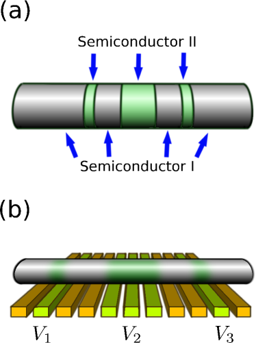
In the present work we focus on the less intensively studied capture dynamics of free electrons into n-doped DQDs mediated solely by long-range electron correlation. Pont et al. (2013) In general the most important electron capture mechanism is via emission of longitudinal optical phonons, that has been studied before in single Glanemann et al. (2005); Jiang et al. (2012) and double QDs. Glanemann et al. (2005) It has been analyzed theoretically in single QDs along with electron collisions and emission. Glanemann et al. (2005); Kvaal (2011) In our previous work Pont et al. (2013) we showed for the first time that electron capture can as well be mediated efficiently by long-range electron correlation in the interatomic Coulombic electron capture (ICEC) in DQDs. The process was named after the one originally predicted to be operative in atoms and molecules. Gokhberg and Cederbaum (2009, 2010) In atoms the electron capture by one atom occurs while another electron is emitted from an atom into its environment. In DQDs the electron capture by one QD leads to an emission of electrons from neighboring QDs with controlled energy properties that can be tuned by changing the geometric DQD parameters. Pont et al. (2013) We postulated ICEC for n-doped DQDs embedded in nanowires (Fig. 1) using an effective mass approximation (EMA) Bastard (1991) based model potential in which we performed numerically exact electron dynamics calculations. The relaxation dynamics of an excitonic electron in undoped materials can be described within the same model provided that the hole relaxation to the band edge has been faster than that of the electron. Narvaez et al. (2006)
We showed already that the probability for ICEC is non-negligible Pont et al. (2013) and can be greatly enhanced in the presence of two-electron resonance states that are capable of undergoing fast ICD-related energy transfer. Here, we systematically add other DQD configurations to those studied before and analyze how and for which energies in the different configurations ICEC in the general and the resonance case becomes most effective.
The paper is organized as follows: First we present some general considerations on the ICEC process (II), introduce our model and the DQD electronic structure (III) followed by the electron dynamics methods used (IV) and the results (V). Since numerically exact computations in the full six-dimensional Hilbert space are very time consuming, we additionally include an effective two-dimensional description of the nanowires and compare to the full dimensional results (V.2.4). The discussion of the results using realistic semiconductor parameters are given in (VI) followed by the conclusions (VII).
II Conditions for ICEC in DQDs
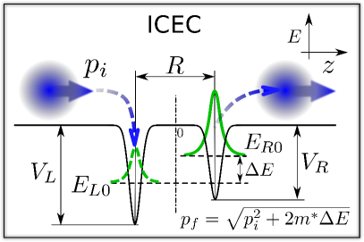
In this work we consider a system of two fully correlated electrons and two QDs which we call the left and right QD and which are described by two different model potentials (see Fig. 2). For the time being consider a left potential well that supports only a single one-electron level with energy and a right one with one single-electron level with energy such that . The tunneling and hybridization between and in the DQD is vanishingly small due to the long interdot distance of the considered system. The ICEC process occurs as depicted in Fig. 2 where an electron is initially bound to the right QD and another electron with momentum is coming in from the left side of the DQD. The incoming electron can then be captured into the ground state of the left QD while the electron on the right is emitted from the ground state of the right QD. Energy conservation dictates that the total energy of the system
| (1) | |||||
| (2) |
is conserved Gokhberg and Cederbaum (2010) and the kinetic energy acquired by the outgoing electron can be expressed as
| (3) |
with the corresponding momentum
| (4) |
where , and is the electron effective mass in atomic units. As one can notice from Eq. (4) the emitted electron can have a higher or a lower momentum than the initial electron, depending on the relation between the bound-state energies and . However, for negative values of the ICEC channel is closed if the incoming electron energy is lower than (see Eq. (4)). Note also that since is the energy acquired by the outgoing electron, then is conversely the energy gain/loss suffered by the DQD.
III Model
The motion of two electrons inside a nanostructured semiconductor can be accurately described using a few-electron effective mass model potential Bastard (1991) in which electron dynamics calculations are feasible. This approach offers then straightforward observability of how electron correlation can lead to ICEC in general two-site systems where electron correlation between moieties plays a fundamental role as well as in the specific case of a QD. We adopt here the model for the DQD used previously to study the dynamics of ICEC Pont et al. (2013); Bande et al. (2015) and ICD. Bande et al. (2011, 2013); Bande (2013) The dots are represented by two Gaussian wells aligned in direction. In and direction we assume a strong harmonic confinement which could be attributed either to depleting gates Fujisawa et al. (1998) or to the actual structure of the semiconductor. Salfi et al. (2010) Besides the full three-dimensional calculations we also considered a simpler one-dimensional model that uses an effective electron-electron interaction to take the wire shape of the system in and direction implicitly into account. In this one-dimensional effective model electron dynamics calculations are much more efficient because only the coordinates of the electrons are evolved in time.
III.1 Hamiltonian
The two-electron effective mass Hamiltonian for the system is
| (5) |
where is the relative dielectric permittivity and
| (6) |
is a one-electron Hamiltonian in which
| (7) | |||||
| (8) |
are the transversal confinement and longitudinal open potentials, respectively. is the effective mass, is the distance between the QDs and are the sizes of the left and right QD while their depths. Performing the scaling of the electronic coordinates one can obtain the scaling relationships of the Hamiltonian parameters shown in Tab. 1. Clearly, we can use the effective mass and the relative permittivity equal to one and rescale the parameters afterwards to obtain the energies and distances for a specific semiconductor.
| Parameter | Scaled value |
|---|---|
| (or ) | |
Due to the comparably strong confinement ( a.u. ) the excited states relevant to this study are only in direction. We will correspondingly have a level structure , in the left (right) QD with energies . The orbital symmetry is simply that of a symmetric well: corresponds to an S-symmetry around the left dot, to a P-symmetry and so on.
III.2 Effective one-dimensional approach
As mentioned in Sec. III.1 the system under consideration has a strong lateral confinement. It is then possible to construct an effective one-dimensional Hamiltonian Bednarek et al. (2003) using the wave function separation ansatz
| (9) |
where are two-dimensional single-electron ground state functions and is the longitudinal effective wave function. Since essentially the same results are obtained for singlet and triplet states, we chose triplet symmetry throughout our study. has the proper symmetry under exchange of electrons given by the longitudinal wave function . The one-dimensional Hamiltonian can be deduced from the analysis of the expectation value of the full Hamiltonian with the product wave function of Eq. (9)
| (10) | |||||
The last term can be explicitly written in the form
| (11) |
with the squared longitudinal wave function and the effective -potential
| (12) |
which depends on , the variable remaining after integrating over the and coordinates.
The size of the two-dimensional ground state wave function is given by and is the distance between the electrons in terms of the confinement size . The asymptotic behavior of exhibits a Coulombic decay behavior at large electron separation. However, at small distances between the electrons this effective potential does not diverge at which is beneficial for numerical treatments:
| (13) | |||||
| (14) |
The validity of the effective potential in different confinement regimes was studied in [Bednarek et al., 2003] for double QDs as a function of the distance between QDs. From Eq. (13) we see that defines the correction order of the effective interaction at large distances. If we take the distance between the dots as a measure of the closest distance that electrons will be from each other, then . We realize then from Eq. (13) that in the regime studied in this work ( and ), the electrons are already in the asymptotic regime of the effective potential. Notice also that the peak at scales as (see Eq. (14)) indicating that in truly narrow confinements () there is less room for the electrons to avoid the divergence of the Coulomb interaction.
IV Computational Details
The dynamical evolution of the system was obtained by solving the time-dependent electronic Schrödinger equation employing the multiconfiguration time-dependent Hartree (MCTDH) approach. Meyer et al. (1990, 2009) The triplet wave function
| (15) |
was expanded in time-dependent single particle functions (SPFs) and coefficients that fulfill the antisymmetry condition for all times. The Dirac-Frenkel variational principle Dirac (1930); Frenkel (1934)
| (16) |
was used to obtain the equations of motion for the coefficients and SPFs.
They were efficiently solved using a constant mean field approach as implemented in the MCTDH-Heidelberg package. Meyer et al. (2009); Beck et al. (2000) The convergence of numerical results was ensured by monitoring the population of the least populated SPF. This is reasonable because the SPFs are adaptive in time and are optimized to describe with the least possible number of SPFs.
The multimode SPFs were in turn expanded in one-dimensional time-dependent SPFs for each of the Cartesian coordinates as
| (17) |
These one-dimensional SPFs are expanded on a DVR-grid (discrete variable representation). We chose harmonic oscillator DVRs for the and , and a sine DVR for the coordinate as listed in Tab. II.
In the full 3D calculations the Coulomb potential was regularized as with to prevent divergences at , and then transformed into sums of products using the POTFIT Beck et al. (2000) algorithm of MCTDH.
A quadratic complex absorbing potential (CAP) was placed at the position along the coordinate to absorb the outgoing electron before it reaches the end of the DVR grid. The CAP obeys
| (18) |
where is the CAP strength and is the Heavyside step function. The absorption prevents the unphysical reflection of outgoing electrons at the grid boundaries.
The absorption of the WP is also used to analyze the energy distribution of the outgoing WP. The quantity that we want to compute is the reaction probability (RP) for ICEC which corresponds to the scattering matrix element which is the probability that an electron impinging from the left on the DQD possessing an electron bound at leads to emission of an electron to the right leaving behind a DQD with an electron bound to .
The computation of the matrix element was performed by using the expression for the stationary scattering eigenfunctions in terms of the initial wave packet Tannor and Weeks (1993) in order to obtain the amount of emitted density from the wave packet absorbed by the CAP. Beck et al. (2000) The energy distribution of the incoming WPi is used to normalize the Fourier transform of the absorbed density to obtain the reaction probability (RP). Beck et al. (2000) We explicitly computed
| (19) |
where
| (20) | |||||
and
| (21) |
where the function is a Gaussian wave packet with a spatial width . is the energy distribution of the incoming WPi peaked around and given by the appropriate Fourier transform which uses the incoming momentum . Tannor and Weeks (1993)
is the absorbed electronic density by the right CAP while another electron is bound in the state. The projectors acting on electron specify which electron is in the state, and the sum over both possible configurations gives the total absorbed density. Note that this quantity explicitly correlates both events, emission and capture, and thus gives only the ICEC contribution of the total emitted density. The scattering matrix in Eq. (19) corresponds to the initial state because the initial wave function
| (22) | |||||
represents a bound electron at plus an incoming electron both in the ground state of the confinement potential.
The RP is a wave-packet independent quantity in the energy range of the size of the energy width of the incoming wavepacket WPi (see Eq. (19)). At each energy, the RP gives the relative amount (in %) of the electron density that would be emitted in the calculation with a monoenergetic electron at that energy. The absorption of WPi by the CAP outside the DQD economizes the computation time needed to obtain the RP.
V Results
In this section we analyze the electronic structure (Sec. V.A) and the dynamics of the electrons (Sec. V.B) in the DQD relevant for ICEC. We compare a number of different configurations that can be classified according to the general setups of the QD model potentials shown in Fig. 3. In setup A only the right QD with a single one-electron state is present. The only purpose of investigating this setup is to prove that, for the incoming electron energies considered in this work, no transmission to the right is possible when the left QD is not present. The configurations belonging to setup B have one left and one right QD and each dot has a single one-electron state, and , respectively. In these cases ICEC is allowed Pont et al. (2013) and occurs as visualized in Fig. 2. Finally, setup C comprises configurations where the left QD has an excited one-electron state in addition to the ground state allowing for the intermediate state to be formed. Since electrons located in the left and right QD are interacting with each other through the long-range Coulomb interaction pushing the state into the continuum, this state turns out to be a two-electron resonance. We will show that under certain conditions this resonance leads to a remarkable increase of the ICEC probability.

V.1 Electronic Structure
As a first step in our analysis we want to study the electronic structure of the DQD embedded in the wire. As explained in Sec. III the two-electron states can be named after the one-electron states of the DQD. The confinement part of the wave function is described by the lowest energy harmonic oscillator wave functions in and both with frequency and effective mass and we therefore concentrate only on the wave function analysis in what follows.
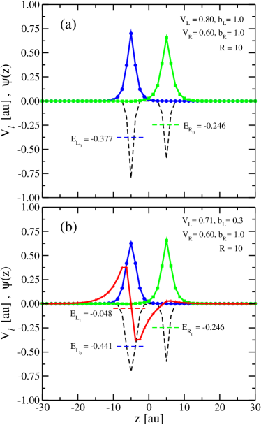
The potential energy curves and the wave functions of the states for two of the configurations used in the dynamical calculations are shown in Fig. 4. The concrete configuration of setup B in Fig. 4(a) has two bound one-electron states and . It is clearly visible that both states are localized in the respective QDs and that there is no hybridization of the states. Two characteristics of this configuration make this possible. One is the distance between the QDs, which is large compared to their size, and the other is the asymmetry of the DQD which leads to different energies for the left and right QDs.
The configuration shown in Fig. 4(b) is a representative of setup C. It shows a wider and shallower left QD which allows for an excited one-electron state . We see that the binding energy is much smaller than and and the wave function is therefore more extended than and .
We set the origin of the energy scale to throughout the study. It amounts to the energy contributed by both electrons in the ground state of the transversal confinement potential (Eq. (7)). With this choice the bound (unbound) states of the longitudinal potential of the DQD have negative (positive) energies.
V.2 Dynamical calculations and results
By employing electron dynamics calculations we can investigate what happens when an electron coming from the left side approaches the DQD where one electron is initially bound and how, if at all, ICEC occurs. We start with the simplest case of setup A (Sec. V.2.1) where only the right QD is present and then move on to different configurations of setup B (Sec. V.2.2) and C (Sec. V.2.3). All examples were computed using both the 1D model (Sec. III.2) and the full 3D Hamiltonian (Sec. III.1) for triplet symmetry. In all cases we chose the energy of the incoming wave packet (WPi) such that it is to low to ionize the electron initially bound to the state, even if the full energy width of the WPi is considered.
V.2.1 One single QD
The initial state of the two-electron systems is an incoming free electron from the left and a bound one in the right QD. A similar setup was studied before, Selstø and Kvaal (2010) however, for a different energy regime of the incoming electron in which two-electron ionization was allowed. The parameters a.u. and a.u. used here give a single bound state with an energy of a.u. The incoming wave packet (WPi) is an energy normalized Gaussian peaked around a.u. The packet has a spatial width a.u. and an energy width a.u. 111The width of the Gaussian wave packet in momentum space is given by . Then the energy width is given by which is not enough to ionize the bound electron by the incoming one. Moreover, excitation to higher states in the transversal directions are energetically forbidden for these parameters.
| DVR type | HO | HO | SIN |
|---|---|---|---|
| DVR points/Primitive Basis | |||
| Range / a.u. | |||
| Grid Spacing (d) / a.u. | |||
| SPFs | ( combined) | ||
| - | - |
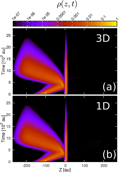
The dynamics of the full 3D scattering process calculated according to the method described in Sec. IV is visualized in Fig. 5(a) by the longitudinal electronic density
| (23) |
as a function of and . The incoming electron is completely reflected starting at about =3 a.u. while the other electron remains bound in the right QD. The same calculation was made using the one-dimensional model described in Sec. III.2 and is shown in Fig. 5(b) for comparison. The evolution is in both cases very similar, only the population of the lowest populated SPF (which is a measure of the convergence as explained in Sec. IV) is different (but however small) in each case giving a value of for the simplified model and for the full calculation. For long times ( a.u.) the total density in the system decreases to zero. The reason for this unphysical behavior is the CAP absorbing the continuum electron. This effect has no impact on the observed results, because the reflection process is already completed within a much shorter time of about 10 a.u.
V.2.2 ICEC in a double quantum dot
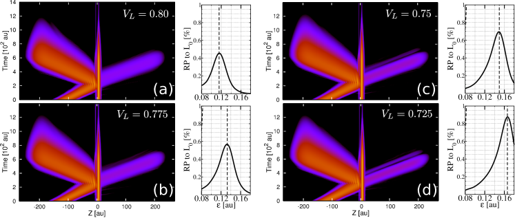
We now focus on configurations of setup B where we added the left QD at a distance a.u. ICEC takes place in these DQDs as depicted in the scheme in Fig. 2 and we confirm this by using different configurations for which Eq. (3) is shown to be fulfilled. The spatially resolved time evolution of of four configurations is shown in each left panel of Fig. 6 (a)-(d). The right QD and the incoming wave packet WPi are the same in all four configurations with a.u., a.u. (same as for setup A before) and a.u., a.u., a.u. The left QD is characterized by a.u., but its depth varies in these configurations taking on the values a.u. The corresponding energies and are given in Tab. 3.
Electron emission to the right is clearly visible in all four cases. The flatter slope of the final wave packet (WPf) trajectory traveling to the right indicates that the emitted electron has higher momentum than the incoming electron. According to Eq. (3) the final energy of the outgoing electron represented by calculated from Eq. (4) (see Tab. 3) decreases when the depth decreases. The RP gives a quantitative measure of ICEC and can be computed using Eq. (19). Descriptively, it is the probability of capturing an electron in the left QD while simultaneously emitting an electron to the right from the right QD. The RP as a function of the incoming electron energy is shown in each right panel of Fig. 6 (a)-(d). The energy range covered in the RP plots is determined by the peak with the energy width of the incoming wave packet. It is possible to obtain reliable results from one simulation within the energy range , which is used for the RP plots.
At this point we would like to discuss more the meaning of the RP. The values given in the plots for ICEC are exactly the amount of the total electron density in percent that would be ejected from to the right and correspondingly the increase of the population of , if the electron incoming from the left was mono-energetic with energy . On the other hand, a mono-energetic electron implies an infinitely wide WPi ( ), which cannot be realized numerically on our finite DVR grid. In our calculations we take a rather broad incoming wavepacket and by employing Eq. (19) we can compute the RP.
Let us analyze the results for RP shown in Fig. 6. They clearly show that ICEC is no at all constant or even monotonic in the covered energy range. On the contrary, it is seen that ICEC is very selective in energy. This is a non-trivial result considering that the ICEC channel into is open for all incoming electron energies (Eq. (4)). The peak of the RP has its origin in the fact that the total energy (see Eqs. (1) and (2)) is the relevant energy in a scattering process. Taylor (2006) The RP shows a marked increase in the probability when the total energy matches the energy gained by the DQD () in the ICEC process in which the emitted electron takes an energy . Using Eq. (1) we obtain the value of at which the peak of the RP is located,
| (24) |
V.2.3 Capture in the presence of a two-electron resonance
The physics of the capture is complicated in the presence of an increased number of bound states of the QDs. In general, several capture and decay channels will be open before and after the capture and the physics of resonance states comes into play. We analyze the probably most simple extension to the DQDs described in the previous sections (setups A and B) by including one extra excited state in the left QD (setup C).
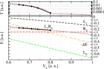
Accordingly, we modify the potential well of the left QD by choosing a.u. instead of a.u., i.e. we make the left well wider. Then we analyze the energies of the states as a function of the depth . This dependence is shown in Fig. 7 for the three-dimensional model. Due to the Coulomb interaction the DQD accommodates a two-electron resonance which derives from the one-electron states and . The resonance energy and decay rate (inverse lifetime) are shown as black dots in Fig. 7. Decay rates in QDs can be computed using different methods. Bande et al. (2011); Cherkes and Moiseyev (2011); Pont et al. (2010) We follow here the approach employed in Bande et al. (2011) in which the resonance state is prepared by imaginary time propagation followed by the real time evolution to find its total decay rate.
The capture process occurs in the presence of the resonance as indicated in Fig. 8 so that different electron capture scenarios can be imagined.
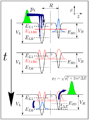
As before in setup B, electron capture into the state with simultaneous release of the other electron from the state is one possible pathway (direct ICEC). Moreover, if the energy of the resonance is above the threshold, the incoming electron can be captured into the two-electron resonance state . After this it decays through a process called interatomic Coulombic decay (ICD), Bande et al. (2011); Cherkes and Moiseyev (2011); Cederbaum et al. (1997); Sisourat et al. (2010a, b); Jahnke et al. (2010) that means by deexcitation of the electron in the left QD (). The released energy is used to emit the electron from the right QD (). Bande et al. (2011) We denote this pathway as the resonance channel and the process as resonance-enhanced ICEC. After being populated by the incoming electron, the resonance can also decay by emitting elastically the electron to the left. This decay resembles that of a shape resonance: Taylor (2006) . This decay is of course only possible when the resonance energy is higher than , a situation that was not usually fulfilled in the systems where ICD was investigated earlier. For completeness we mention that the incoming electron energy is sufficiently low so that direct electron capture into the state is energetically forbidden for all cases considered here.
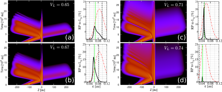
The time evolution of the electron density has been calculated for different left well depths 0.65, 0.67, 0.71, and 0.74 a.u. (Fig. 9, left panels). Comparing with the results for setup B (Fig. 6) a clear difference is observed for the density emitted from to the right. In setups a continuous decay with an exponential time constant is visible while an almost instantaneous electron emission takes place for setups . This indicates that the mechanisms involved in the capture and emission processes are different for both setups. It is also noteworthy that the emitted electronic density to the left becomes more complex in case showing clear signatures of interference with the incoming WPi. The electron emitted elastically to the left is responsible for these interference effects.
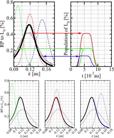
The results obtained for ICEC in section V.2.2 show that the ICEC probability is highest if the total energy matches the negative of the energy difference . It is, therefore, worthwhile to study the behavior of the ICEC probability in relation to the value of in the presence of a resonance. Fig. 7 shows that the resonance energy crosses around the value a.u. We previously addressed the configuration with a.u. which is near the crossing point of the energies . Pont et al. (2013) In this case, the coincidence of the RP peak and the resonance energy lead to an extraordinary increase of the ICEC probability. The presence of the resonance enables an extra channel that can be tuned to cooperatively augment the emission. The RP for this and three other values belonging to configurations above and below the mentioned crossing point are shown in the right panels of Fig. 9. The incoming WPi also depicted in Fig. 9 is different for each of the configurations because the RP region of interest changes with the resonance energy. Nevertheless, the energy range shown is the same in the four plots.
We observe that for and a.u. the RP develops one large peak with a shoulder indicating a second peak. These two peaks correspond to the direct and the resonance-enhanced ICEC channels of the scattering process. The vertical lines depicted in the corresponding panels of Fig. 9 stand for the energy of the resonance and of the ICEC peak computed from Eq. (24). The maxima of the RP are seen to be slightly displaced from these lines. In this sense the simple picture of independent resonance and direct ICEC peaks is not strictly valid and a correction taking the interaction between them into account is needed in order to obtain the correct peak positions. It should also be clear that both channels may interfere. It is noteworthy that the RPs now take on values of 10 and 16 %, respectively, which are substantially higher than in the case of setup B where only the direct ICEC channel is operative.
The choice of a.u. in panel (c) provides an extraordinary increase of the capture and emission probability. This probability of 22 % indicates that the direct and resonance ICEC pathways coherently contribute to the same channel . The peak height strongly depends on whether the values of and (depicted in Fig. 9 and listed in Tab. 4) coincide. We see in Fig. 9 for case (d) where is slightly enhanced that the peak height, now about 5 %, is again smaller than in case (c). Clearly, the increase of the ICEC probability in case (c) derives from the concurrence of both processes. The total width of the RP peak for case (c) is very narrow and given by the inverse lifetime of the resonance, as opposed to the other cases where a wider RP with more than one peak is obtained. This narrowness can be utilized to design an energy selective device. Pont et al. (2013)
In case (c) the emitted electron density reaches the grid boundary before the resonant emission from the DQD has terminated. This has no effect on the RP values as we find when using longer grids where the full emission is possible before reaching the absorbing boundary. This is demonstrated explicitly in the following section.
V.2.4 ICEC in the one-dimensional effective model
In addition to the results given by the full three-dimensional simulations we performed computations using the one-dimensional model described in section III.2. These calculations are much less time consuming and also allow to use much larger grids.
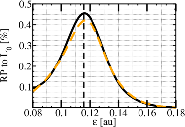
The result for configuration (a) of Setup B is shown in Fig. 10 demonstrating that the RP is structurally and quantitatively similar to that of the full three-dimensional computation. Without showing the picture we note that also the evolution of the electron density in the one-dimensional effective model is very similar to that of Fig. 6 for the full three-dimensional computation.
Since the computation times are considerably reduced for the one-dimensional model, we can perform the simulations on much longer grids than those used for the 3D calculations. Now, we can address numerically the question whether the RP obtained from Eq. (19) reproduces the population of the state via ICEC computed by employing incoming mono-energetic electrons. The initial wave packet WPi can now be chosen to be spatially wider with a.u., with a reduced dispersion in energy a.u. As indicated in Sec. V.2.3, the maximum population of the state over time can now be computed for a selected value of the energy of the incoming electron. This determines the RP at that energy. Clearly, we need to repeat the simulation using different incoming energies in order to construct a full RP curve. An example of an RP curve constructed in this manner is depicted in Fig. 11. We observe that the maxima of the populations follow closely the values of the RPs obtained from the flux determined via Eq. (19), even though the energy distributions of the WPis used to describe mono-chromatic incoming electrons are not extremely narrow as they should be. If they were infinitely narrow, then we would expect both RP results to coincide.
The RP does not change if we use different WPs. We can demonstrate this by using an energetically narrow wave packet with a.u. to compute the RPs and comparing the result with the RPs computed using a wide WP with a.u. The lower panels in Fig. 11 show that the respective RP curves compare very well in the energy regions where both curves are valid.
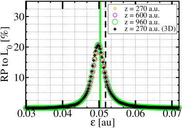
The comparison of the full 3D and the one-dimensional model for setup C is shown in Fig. 12. We chose the parameters of configuration (c) of Fig. 9, where the greatest RP due to resonance-enhanced ICEC occurs. As for setup B, the evolution of the electronic density is very similar to that of Fig. 9(c) and the RP is almost identical.
The one-dimensional RPs were computed for three different grid lengths, and no difference with the results of the computed full 3D RPs ( a.u.) is observed for grids up to a.u. This shows that the RP is a robust and reliable quantity which is independent of the WP used and, to a great extent, also of the grid size. This important point is further discussed below.
In principle, one could estimate the RP for a given energy by studying the populations or of the one-electron states and of the left and right QDs computed using an energetically narrow WP and a long grid. For setup B this estimate works well as we did use a narrow WP. For setup C, however, we used in the full 3D calculations an energetically wide WP and a rather short grid and one cannot expect the above mentioned estimate to produce realistic results. Indeed, our calculations of these populations and of the norm of the wave packet show that these quantities decay due to absorption into the boundaries of the grid before the estimate takes on the correct value. This is mainly because the WP used is very wide. This raises the question on why is then the RP computed employing Eq. (19) not affected by the grid size as is demonstrated in Fig. 12. The answer is that this equation keeps collecting the flux on the boundary as long as the population on the right QD decreases and that of the left QD, , increases (see Eqs. (19-20). Clearly, absorption on the boundaries does not affect the RP of ICEC when computed via these equations. In other words, the RP is very robust against absorption and this also explains the insensitivity of the results to the size of the grid and width of the wave packet as found above.
The results show that the overall density evolution is very similar and the 1D model provides very good results for the RP in both setups B and C. Moreover, sometimes it is only possible to perform one-dimensional computations using grids long enough to show the complete ICEC process. This assertion strongly supports the use of one-dimensional effective models when is low and thus is not able to produce excitations in the lateral confinement. The one-dimensional model is a very useful tool if the RPs of many different configurations needs to be analyzed, because it allows to quickly identify the relevant energy range and shape of the RPs.
VI Discussion
We demonstrated that ICEC is operative and in some cases a very effective electron capture mechanism in DQDs. In the previous sections we have shown how a simple full-dimensional model can be constructed to describe the process. Nevertheless, our model includes only electron correlation to mediate electron capture, although other capture mechanisms are likely to be as effective as ICEC. Therefore we stick to an estimation on the importance of ICEC with respect to other processes. As we will show, the capture times for ICEC are in the same order or even faster than other common mechanisms.
The capture rate into QDs is the commonly used quantity to characterize the efficiency of an electron capture process and it depends strongly on the amount of time it takes for the capture to be completed, i. e. a faster capture leads to a greater efficiency. The importance of ICEC is then determined by comparing the time it takes ICEC to complete capture compared to the electron capture times reported for other processes available in the system. Prasankumar et al. (2009); Porte et al. (2009); Sauvage et al. (2002); Robel et al. (2006)
To estimate the speed of ICEC we transfer the parameters of our model to realistic semiconductor structures using the effective mass conversion of Table 1. It is applicable to gate defined DQDs with quasi-one dimensional geometry Fasth et al. (2005); Fujisawa et al. (1998) or to QDs embedded in nanowires, Salfi et al. (2010) so we compare ICEC times with those obtained for other capture processes in these systems. Table 5 shows the energies and sizes for different materials in setup B, case (a) and Table 6 those for setup C, case (c). The energies obtained are well in the range of intraband level spacings of QDs in nanowires Salfi et al. (2010); Roddaro et al. (2011) and of intrashell levels in self-assembled QDs. Zibik et al. (2009)
Let us first analyze setup B. The time window shown in Fig. 6 is about a.u. and by transforming to SC materials of Table 5 we obtain , , , ps. The time it takes the ICEC process to capture and emit the electron can be estimated from the reaction probability if we take into account the time-energy uncertainity and the fact that the process gives a peak-shaped RP. The RP line shape can then be fitted to a Breit-Wigner resonance line shape. We performed such a fitting and find for case (a) au, and the times in different materials are accordingly: , , and ps. We stress that this time estimation only makes sense because we obtained a resonant behavior, rather than a non zero contribution for all energy values.
The surprisingly short time scale it takes ICEC to occur makes ICEC a promising mechanism competitive with other capture processes. It is faster than the reported capture times of ps for free carriers in bulk GaAs into InAs/GaAs QDs in single layer samples measured at room temperature Turchinovich et al. (2003).
The time scale of ICEC obtained for the different geometries always gives shorter times for smaller sizes of the DQD. This fact stresses the importance of confinement for the process to be competitive. It can be connected to previous studies on ICD in molecular dimers, where the length scale of about nm typically corresponds to lifetimes in the range of several fs. Cederbaum et al. (1997)
. Parameter GaAs InP AlN InAs 9.79 8.99 1.12 28.61 3.86 3.70 1.58 6.08 9.48 4.87 120.52 2.76 7.11 7.75 90.39 2.07 -4.47 -4.87 -56.78 -1.30 -2.92 -3.18 -37.10 -0.85
| Parameter | GaAs | InP | AlN | InAs |
|---|---|---|---|---|
| 17.88 | 16.41 | 2.05 | 52.24 | |
| 9.79 | 8.99 | 1.12 | 28.61 | |
| 3.86 | 3.70 | 1.58 | 6.08 | |
| 8.42 | 9.17 | 106.96 | 2.45 | |
| 7.11 | 7.75 | 90.39 | 2.07 | |
| -5.23 | -5.69 | -66.40 | -1.52 | |
| -2.92 | -3.18 | -37.10 | -0.85 | |
| 0.57 | 0.62 | 7.19 | 0.16 |
For the setup C case (c) the time window shown in Fig. 9 is of a.u. and transforming it to the semiconductor materials of Table 5 we obtain , , , ps. We can in this setup estimate the duration of the emission using the lifetime of the involved resonance . We have that for case (c) a.u. which gives the following times in real semiconductors , , , ps. From the observed values of the GaAs energy spacings and electron energies in the range of meV, the decay of the L1R0 resonance in ICEC seems to be competitive with relaxation via phonons. The times for ICEC are, however, faster than reported intraband decay times due to acoustic phonon emission for InGaAs/GaAs QDs of ps. Zibik et al. (2009)
Our work is focused on strongly laterally confined structures, such as nanowires, and is thus suitable for the use of a one-dimensional effective potential. In all cases and setups treated here both the full and one-dimensional descriptions provided almost identical qualitative and quantitative results. The main result obtained from this comparison for the cases studied in this work is that the physics in the strongly laterally confined model can be correctly described using the effective potential when the characteristic lateral energies are about twice or more than those of the QDs.
VII Conclusions
Ultrafast electron capture in single QDs is an extensively studied topic nowadays Nozik et al. (2010); Prasankumar et al. (2009); Porte et al. (2009) due to its relevance in the development of a wide variety of technological applications. Prasankumar et al. (2009); Porte et al. (2009); Narvaez et al. (2006) As shown here, electron capture via the ICEC processes, in which the neighboring QD in a DQD is getting ionized, is particularly fast and can play a significant role in the dynamics contributing to the energy transfer between QDs. The ICEC mechanisms in DQDs could, in principle, be exploited to be implemented in devices which generate a nearly monochromatic low energy electron in a given direction.
The implementation of DQDs in nanowires using materials with long carrier lifetimes such as InP Prasankumar et al. (2009); Roddaro et al. (2011) should be favorable for ICEC. The rate at which the electron capture occurs varies with material and radius of the wire. Reported times for carrier trapping cover a large range from fast values of ps for GaAs Parkinson et al. (2007) and ps for ZnO Prasankumar et al. (2009) to very slow ones such as ns for InP nanowires. Titova et al. (2007) Using wires with long carrier trapping times are favorable for ICEC to be active.
The process is driven by long-range Coulomb interactions, so we expect ICEC to be also applicable to other QDs geometries like, e.g., self-assembled vertically stacked dots. Müller et al. (2012); Benyoucef et al. (2012); Porte et al. (2009); Zibik et al. (2009)
We have derived an effective one-dimensional approach that correctly describes the dynamics and RPs of all the cases we have considered. This approach reduces considerably the computational efforts and also demonstrates, by comparison with full 3D computations, that the physics involved is described correctly by a one-dimensional model as long as the characteristic confinement energy is about twice or more than that of the QD.
The calculations presented were performed for the same distance between the dots. Since long-range correlation is involved in ICEC a rather pertinent question is how the reaction probability changes with . The answer has been partially given in the first publications on ICEC in atoms and molecules (see Ref. Gokhberg and Cederbaum, 2010) and for the related ICD decay (see Refs. Bande et al., 2011 and Bande et al., 2013). The ICEC cross section has an asymptotic decay with the distance, according to previous theoretical estimates for atoms and molecules. However, there are important contributions not considered in the asymptotic formulas leading to which are due to orbital overlap (see, Ref. Bande et al., 2011 for ICD in QDs and Ref. Averbukh et al., 2004 for molecules). These contributions can lead in some cases to a much faster ICD process. Furthermore, the quasi-one dimensional geometry of the dots considered here has a clear influence on ICD (Ref. Bande et al., 2011) and probably also on ICEC. The calculations are rather cumbersome and at the moment there is no exhaustive analysis of this kind for ICEC, but it will be done in the future.
VIII Acknowledgments
F. M. P. acknowledges financial support by Deutscher Akademischer Austauschdienst (DAAD) and Consejo Nacional de Investigaciones Científicas y Técnicas (CONICET) and A. B. by Heidelberg University (Olympia-Morata fellowship) as well as Volkswagen foundation (Freigeist fellowship). L.S.C. and A.B. thank the Deutsche Forschungsgemeinschaft (DFG) for financial support.
References
- AlAhmadi (2012) A. AlAhmadi, Quantum Dots - A Variety of New Applications (InTech, Open Acces, 2012).
- Fujisawa et al. (1998) T. Fujisawa, T. H. Oosterkamp, W. G. van der Wiel, B. W. Broer, R. Aguado, S. Tarucha, and L. P. Kouwenhoven, Science 282, 932 (1998).
- Shabaev et al. (2006) A. Shabaev, A. L. Efros, and A. J. Nozik, Nano Lett. 6, 2856 (2006).
- Müller et al. (2012) K. Müller, A. Bechtold, C. Ruppert, M. Zecherle, G. Reithmaier, M. Bichler, H. J. Krenner, G. Abstreiter, A. W. Holleitner, J. M. Villas-Boas, M. Betz, and J. J. Finley, Phys. Rev. Lett. 108, 197402 (2012).
- Benyoucef et al. (2012) M. Benyoucef, V. Zuerbig, J. P. Reithmaier, T. Kroh, A. W. Schell, T. Aichele, and O. Benson, Nanoscale Res. Lett. 7, 493 (2012).
- van der Wiel et al. (2002) W. G. van der Wiel, S. De Franceschi, J. M. Elzerman, T. Fujisawa, S. Tarucha, and L. P. Kouwenhoven, Rev. Mod. Phys. 75, 1 (2002).
- Salfi et al. (2010) J. Salfi, S. Roddaro, D. Ercolani, L. Sorba, I. Savelyev, M. Blumin, H. E. Ruda, and F. Beltram, Semicond. Sci. Technol. 25, 024007 (2010).
- Laird et al. (2010) E. A. Laird, J. M. Taylor, D. P. DiVincenzo, C. M. Marcus, M. P. Hanson, and A. C. Gossard, Phys. Rev. B 82, 075403 (2010).
- Roddaro et al. (2011) S. Roddaro, A. Pescaglini, D. Ercolani, L. Sorba, and F. Beltram, Nano Lett. 11, 1695 (2011).
- Nadj-Perge et al. (2012) S. Nadj-Perge, V. S. Pribiag, J. W. G. van den Berg, K. Zuo, S. R. Plissard, E. P. A. M. Bakkers, S. M. Frolov, and L. P. Kouwenhoven, Phys. Rev. Lett. 108, 166801 (2012).
- Reed et al. (1988) M. A. Reed, J. N. Randall, R. J. Aggarwal, R. J. Matyi, T. M. Moore, and A. E. Wetsel, Phys. Rev. Lett. 60, 535 (1988).
- Kastner (1993) M. A. Kastner, Phys. Tod. 46, 24 (1993).
- Goldstein et al. (1985) L. Goldstein, F. Glas, J. Y. Marzin, M. N. Charasse, and G. L. Roux, Appl. Phys. Lett. 47, 1099 (1985).
- Henini (2011) M. Henini, Handbook of self assembled semiconductor nanostructures for novel devices in photonics and electronics (Elsevier, 2011).
- Gur et al. (2005) I. Gur, N. A. Fromer, M. L. Geier, and A. P. Alivisatos, Science 310, 462 (2005).
- Nozik et al. (2010) A. J. Nozik, M. C. Beard, J. M. Luther, M. Law, R. J. Ellingson, and J. C. Johnson, Chem. Rev. 110, 6873 (2010).
- Fujita et al. (2013) T. Fujita, H. Kiyama, K. Morimoto, S. Teraoka, G. Allison, A. Ludwig, A. D. Wieck, A. Oiwa, and S. Tarucha, Phys. Rev. Lett. 110, 266803 (2013).
- Studenikin et al. (2012) S. A. Studenikin, G. C. Aers, G. Granger, L. Gaudreau, A. Kam, P. Zawadzki, Z. R. Wasilewski, and A. S. Sachrajda, Phys. Rev. Lett. 108, 226802 (2012).
- Porte et al. (2009) H. P. Porte, P. Uhd Jepsen, N. Daghestani, E. U. Rafailov, and D. Turchinovich, Appl. Phys. Lett. 94, 262104 (2009).
- Leturcq et al. (2009) R. Leturcq, C. Stampfer, K. Inderbitzin, L. Durrer, C. Hierold, E. Mariani, M. G. Schultz, F. von Oppen, and K. Ensslin, Nat. Phys. 5, 327 (2009).
- Prasankumar et al. (2009) R. P. Prasankumar, P. C. Upadhya, and A. J. Taylor, Phys. Status Solidi B 246, 1973 (2009).
- Zibik et al. (2009) E. A. Zibik, T. Grange, B. A. Carpenter, N. E. Porter, R. Ferreira, G. Bastard, D. Stehr, S. Winnerl, M. Helm, H. Y. Liu, M. S. Skolnick, and L. R. Wilson, Nat. Mater. 8, 803 (2009).
- Narvaez et al. (2006) G. A. Narvaez, G. Bester, and A. Zunger, Phys. Rev. B 74, 075403 (2006).
- Shirasaki et al. (2013) Y. Shirasaki, G. J. Supran, M. G. Bawendi, and V. Bulović, Nat. Photonics 7, 13 (2013).
- Bande et al. (2011) A. Bande, K. Gokhberg, and L. S. Cederbaum, J. Chem. Phys. 135, 144112 (2011).
- Bande et al. (2013) A. Bande, F. M. Pont, P. Dolbundalchok, K. Gokhberg, and L. S. Cederbaum, EPJ Web Conf. 41, 04031 (2013).
- Cherkes and Moiseyev (2011) I. Cherkes and N. Moiseyev, Phys. Rev. B 83, 113303 (2011).
- Bande (2013) A. Bande, J. Chem. Phys. 138, 214104 (2013).
- Cederbaum et al. (1997) L. S. Cederbaum, J. Zobeley, and F. Tarantelli, Phys. Rev. Lett. 79, 4778 (1997).
- Sisourat et al. (2010a) N. Sisourat, H. Sann, N. V. Kryzhevoi, P. Kolorenč, T. Havermeier, F. Sturm, T. Jahnke, H.-K. Kim, R. Dörner, and L. S. Cederbaum, Phys. Rev. Lett. 105, 173401 (2010a).
- Sisourat et al. (2010b) N. Sisourat, N. V. Kryzhevoi, P. Kolorenč, S. Scheit, T. Jahnke, and L. S. Cederbaum, Nat. Phys. 6, 508 (2010b).
- Jahnke et al. (2010) T. Jahnke, H. Sann, T. Havermeier, K. Kreidi, C. Stuck, M. Meckel, M. Schöffler, N. Neumann, R. Wallauer, S. Voss, A. Czasch, O. Jagutzki, A. Malakzadeh, F. Afaneh, T. Weber, H. Schmidt-Böcking, and R. Dörner, Nat. Phys. 6, 139 (2010).
- Pont et al. (2013) F. M. Pont, A. Bande, and L. S. Cederbaum, Phys. Rev. B 88, 241304(R) (2013).
- Glanemann et al. (2005) M. Glanemann, V. M. Axt, and T. Kuhn, Phys. Rev. B 72, 045354 (2005).
- Jiang et al. (2012) F. Jiang, J. Jin, S. Wang, and Y.-J. Yan, Phys. Rev. B 85, 245427 (2012).
- Kvaal (2011) S. Kvaal, Phys. Rev. A 84, 022512 (2011).
- Gokhberg and Cederbaum (2009) K. Gokhberg and L. S. Cederbaum, J. Phys. B: At. Mol. Opt. 42, 231001 (2009).
- Gokhberg and Cederbaum (2010) K. Gokhberg and L. S. Cederbaum, Phys. Rev. A 82, 052707 (2010).
- Bastard (1991) G. Bastard, Wave Mechanics Applied to Semiconductor Heterostructures, Monographs of Physics (Les Editions de Physique) No. 1 (Wiley, John & Sons, Inc., Les Ulis Cedex, France, 1991).
- Bande et al. (2015) A. Bande, F. M. Pont, K. Gokhberg, and L. S. Cederbaum, EPJ Web of Conferences 84, 07002 (2015).
- Bednarek et al. (2003) S. Bednarek, B. Szafran, T. Chwiej, and J. Adamowski, Phys. Rev. B 68, 045328 (2003).
- Meyer et al. (1990) H.-D. Meyer, U. Manthe, and L. Cederbaum, Chem. Phys. Lett. 165, 73 (1990).
- Meyer et al. (2009) H.-D. Meyer, F. Gatti, and G. A. Worth, Multidimensional Quantum Dynamics: MCTDH Theory and Applications (John Wiley & Sons, Weinheim, 2009).
- Dirac (1930) P. A. M. Dirac, Math. Proc. Cambridge 26, 376 (1930).
- Frenkel (1934) J. Frenkel, Wave Mechanics: Advanced General Theory (The Clarendon Press, Oxford, 1934).
- Beck et al. (2000) M. H. Beck, A. Jäckle, G. A. Worth, and H. D. Meyer, Phys. Rep. 324, 1 (2000).
- Tannor and Weeks (1993) D. J. Tannor and D. E. Weeks, J. Chem. Phys. 98, 3884 (1993).
- Selstø and Kvaal (2010) S. Selstø and S. Kvaal, J. Phys. B: At. Mol. Opt. Phys. 43, 065004 (2010).
- Note (1) The width of the Gaussian wave packet in momentum space is given by . Then the energy width is given by .
- Taylor (2006) J. R. Taylor, Scattering Theory: The Quantum Theory of Nonrelativistic Collisions (Dover Publications, Mineola, New York, 2006).
- Pont et al. (2010) F. M. Pont, O. Osenda, J. H. Toloza, and P. Serra, Phys. Rev. A 81, 042518 (2010).
- Sauvage et al. (2002) S. Sauvage, P. Boucaud, R. P. S. M. Lobo, F. Bras, G. Fishman, R. Prazeres, F. Glotin, J. M. Ortega, and J.-M. Gérard, Phys. Rev. Lett. 88, 177402 (2002).
- Robel et al. (2006) I. Robel, B. A. Bunker, P. V. Kamat, and M. Kuno, Nano Lett. 6, 1344 (2006).
- Fasth et al. (2005) C. Fasth, A. Fuhrer, M. T. Björk, and L. Samuelson, Nano Lett. 5, 1487 (2005).
- Turchinovich et al. (2003) D. Turchinovich, K. Pierz, and P. Uhd Jepsen, Phys. Status Solidi C 0, 1556 (2003).
- Singh (1993) J. Singh, Physics of semiconductors and their heterostructures (McGraw-Hill, New York, 1993).
- Levinshtein et al. (2001) M. E. Levinshtein, S. L. Rumyantsev, and M. S. Shur, Properties of Advanced Semiconductor Materials: GaN, AIN, InN, BN, SiC, SiGe (John Wiley & Sons, New York, 2001).
- Parkinson et al. (2007) P. Parkinson, J. Lloyd-Hughes, Q. Gao, H. H. Tan, C. Jagadish, M. B. Johnston, and L. M. Herz, Nano Lett. 7, 2162 (2007).
- Titova et al. (2007) L. V. Titova, T. B. Hoang, J. M. Yarrison-Rice, H. E. Jackson, Y. Kim, H. J. Joyce, Q. Gao, H. H. Tan, C. Jagadish, X. Zhang, J. Zou, and L. M. Smith, Nano Lett. 7, 3383 (2007).
- Averbukh et al. (2004) V. Averbukh, I. B. Müller, and L. S. Cederbaum, Phys. Rev. Lett. 93, 263002 (2004).