Star-forming galaxies as the origin of the IceCube PeV neutrinos

Abstract

Star-forming galaxies, due to their high star-formation rates and hence large number of supernova remnants therein, are huge reservoirs of cosmic rays (CRs). These CRs collide with gases in the galaxies and produce high-energy neutrinos through $pp$ collisions. In this paper, we calculate the neutrino production efficiency in star-forming galaxies by considering realistic galaxy properties, such as the gas density and galactic wind in star-forming galaxies. To calculate the accumulated neutrino flux, we use the infrared luminosity function of star-forming galaxies obtained by Herschel PEP/HerMES survey recently. The intensity of CRs producing PeV neutrinos in star-forming galaxies is normalized with the observed CR flux at EeV ( 1 EeV=$10^{18}\,$eV), assuming that supernova remnants or hypernova remnants in star-forming galaxies can accelerate protons to EeV energies. Our calculations show that the accumulated neutrino emission produced by CRs in star-forming galaxies can account for the flux and spectrum of the sub-PeV/PeV neutrinos under reasonable assumptions on the CR confinement time in these galaxies.

1. Introduction

The IceCube Collaboration recently announced the discovery of extraterrestrial neutrinos. With 37 events ranging from 60 TeV to 3 PeV within three years of operation, the excess over the background atmospheric neutrinos and muons reaches 5.7$\sigma$ (Aartsen et al., 2014). The non-detection of events beyond 3 PeV suggests that the neutrino flux follows either a hard power law spectrum with a break above 3 PeV, or an unbroken power law spectrum with a softer index of $\Gamma\simeq 2.2-2.3$ (Aartsen et al., 2014; Anchordoqui et al., 2014a; Winter, 2014). The sky distribution of these events is consistent with isotropy (Aartsen et al., 2014), implying that an extragalactic origin is dominant, although a fraction of them could come from Galactic sources (Fox et al., 2013; Razzaque, 2013; Lunardini et al., 2014; Ahlers & Murase, 2014; Neronov et al., 2014).

The source of the IceCube neutrinos is still controversial. The proposed astrophysical sources include starburst and star-forming galaxies (Loeb & Waxman, 2006; Liu et al., 2014; He et al., 2013; Murase et al., 2013; Tamborra et al., 2014; Anchordoqui et al., 2014b; Wang et al., 2014), gamma-ray bursts (Waxman & Bahcall, 1997; Murase & Ioka, 2013; Cholis & Hooper, 2013; Liu & Wang, 2013), and jets and/or cores of active galactic nuclei (AGNs) (Anchordoqui et al., 2008; Kalashev et al., 2013; Stecker, 2013; Dermer et al., 2014), newborn pulsars (Fang et al., 2014) and etc. In this paper, we focus on the scenario of starburst/star-forming galaxies, where cosmic rays (CRs) therein collide with dense gases in intersteller medium and produce neutrinos. The gamma-ray observations of nearby star-forming galaxies by Fermi Large Area Telescope (LAT), including M31, LMC, SMC, M82, NGC 253 and NGC 2146 (Ackermann et al., 2012; Tang et al., 2014), have proven that $pp$ collisions occur in such star-forming galaxies, so they are guaranteed factories of high-energy neutrinos.

In the pioneering work of the starburst galaxy scenario, Loeb & Waxman (2006) assume that CRs in the starburst galaxies lose almost all the energy into pions and calibrate the GeV neutrino emissivity with the synchrotron radio emissivity. A simple power-law extrapolation is then used to estimate the neutrino flux at PeV energies. On the other hand, we (Liu et al., 2014) studied the PeV neutrino emissions from star-forming/starburst galaxies, assuming that the intensity of CRs producing PeV neutrinos in star-forming/starburst galaxies matches the observed CR flux at EeV. This is motivated by the possibility that PeV neutrinos could originate from the same sources responsible for extragalactic CRs (Liu et al., 2014), as PeV neutrinos require $\sim 50$ PeV CRs, which is only one order of magnitude lower than the energy of the ”second knee” of CR spectrum ($4-8\times 10^{17}\mathrm{eV}$), where the transition from Galactic CRs to extragalactic CRs may occur (Berezinsky et al., 2006). It has been suggested that the remnants of hypernovae or other peculiar types of supernovae in star-forming galaxies may accelerate protons to EeV energies due to their faster ejecta and larger explosion energy (Wang et al., 2007; Budnik et al., 2008; Chakraborti et al., 2011; Liu & Wang, 2012). In Liu et al. (2014), we assume that all star-forming galaxies as well as all starburst galaxies have uniform properties such as gas density, which lead to the same neutrino production efficiency among all star-forming galaxies, and among all starburst galaxies. However, the CR intensity and gas density should be different in galaxies of different luminosities or types. In this paper, we attempt to improve our earlier calculation by considering realistic galaxy properties and the galaxy luminosity function. The luminosity function describes the relative number of galaxies of different luminosities, as well as the evolution of a galaxy population with redshift. The Herschel PEP/HerMES survey has recently provided an estimate of the IR luminosity function up to $z\sim 4$ (Gruppioni et al., 2013). It also enables people to estimate the luminosity functions of specific galaxy populations: normal spiral galaxies, starbursts and star-forming galaxies containing obscured or low-luminosity AGNs, all of which contribute to the star-formation rate in the Universe (Gruppioni et al., 2013). The gas density in a galaxy is expected to relate to its star-formation rate and hence to the IR luminosity of the galaxy. Then, with these galaxy properties known, we are able to calculate the neutrino fluxes produced in star-forming galaxies of different luminosities and populations.

In §2, we first outline the neutrino production process in star-forming galaxies. In §3, we describe the galaxy parameters that are needed for calculating the accumulated neutrino flux from star-forming galaxies. In §4, we invoke the luminosity function to calculate the accumulated neutrino flux produced by all the star-forming galaxies in the Universe. Finally, we give our conclusions and discussions in §5.

2. Neutrino production process in star-forming galaxies

Supernova remnants (SNRs)are widely discussed as accelerators of CRs. Due to high star-formation rates (SFRs) in star-forming galaxies, large amount of SNRs reside in these galaxies and hence these galaxies are huge reservoirs of CRs. The total energy of CRs injected into a galaxy per unit time is proportional to the total SFR of the galaxy, i.e., $L_{p}\propto\mathrm{SFR}$, where $L_{p}$ represents the luminosity in CR protons. The total infrared luminosity of a galaxy is a good tracer for its SFR, and there exists a widely used relation between the total infrared luminosity $L_{\text{TIR}}$ and SFR (Kennicutt, 1998). Thus we expect that $L_{p}\propto L_{\mathrm{TIR}}$, i.e.

$$L_{p}=C\frac{L_{\mathrm{TIR}}}{L_{\odot}}\left(\frac{E_{p}}{1\mathrm{GeV}}\right)^{-p},$$ (1)

where $C$ is the normalization factor, $L_{\odot}$ is the bolometric luminosity of the Sun and $E_{p}$ is the proton energy in unit of GeV. $p$ is the index of the proton spectrum ($dn/dE_{p}\propto E_{p}^{-p}$), and we assume $p=2$, as expected from the first-order Fermi acceleration in blastwaves of SNRs.

Once the accelerated CRs are injected into interstellar medium (ISM), hadronuclear collisions between CRs and nuclei in ISM would produce charged pions, which will decay to neutrinos ($\pi^{+}\rightarrow\nu_{\mu}\bar{\nu}_{\mu}\nu_{e}e^{+},\,\pi^{-}\rightarrow\bar{\nu}_{\mu}\nu_{\mu}\bar{\nu}_{e}e^{-}$). On the other hand, CRs can escape a galaxy through diffusion or galactic wind advection. These two competing processes regulate the efficiency of the pion-production of CRs which can be described by $f_{\pi}=1-\exp\left(-t_{\text{esc}}/t_{\text{loss}}\right)$, where $t_{\text{esc}}$ is the escape time of CRs and $t_{\text{loss}}$ is the energy-loss time of CRs via proton–proton ($pp$) collisions.

The energy-loss time $t_{\text{loss}}$ can be expressed as $\left(0.5n\sigma_{pp}c\right)^{-1}$, where 0.5 is the inelasticity factor, $n$ is the particle number density and $\sigma_{pp}$ is the inelastic $pp$ collision cross section. We convert the particle number density to gas surface density by $\Sigma_{g}=m_{p}nH$, where $m_{p}$ is the mass of proton and $H$ is the height of the galaxy, the energy-loss time is

$$t_{\text{loss}}=1.4\times 10^{5}\frac{H}{1\text{kpc}}\left(\frac{\sigma_{pp}}{70\text{mb}}\right)^{-1}\left(\frac{\Sigma_{g}}{1\text{g cm}^{-2}}\right)^{-1}\text{yr}.$$ (2)

There are basically two ways for CRs to escape from a galaxy, i.e. diffusion and advection. In the diffusion escape case, CRs are scattered by small-scale inhomogeneous magnetic fields randomly and diffuse out of the host galaxy. The diffusive escape time is $t_{\text{diff}}=H^{2}/4D$. Here $D=D_{0}\left(E/E_{0}\right)^{\delta}$ is the diffusion coefficient, where $D_{0}$ and $E_{0}={\rm 3GeV}$ are normalization factors, and $\delta=0-1$ depending on the spectrum of interstellar magnetic turbulence. The diffusion time is

$$t_{\text{diff}}=7.5\times 10^{6}\left(\frac{H}{1\text{kpc}}\right)^{2}\left(\frac{D_{0}}{10^{28}\text{cm}^{2}\text{s}^{-1}}\right)^{-1}\left(\frac{E_{p}}{3\text{GeV}}\right)^{-\delta}\text{yr}.$$ (3)

Since galaxies with higher IR luminosities are observed to have stronger magnetic fields (Thompson et al., 2006), and the diffusion coefficient is expected to scale with the CR Larmor radius, these high luminosity galaxies could have a smaller diffusion coefficient. Thus, we allow lower values of diffusion coefficient for galaxies with IR luminosity $L_{\text{TIR}}>10^{11}L_{\odot}$ in the calculation, while the diffusion coefficient for galaxies with IR luminosity $L_{\text{TIR}}<10^{11}L_{\odot}$ is fixed to $D_{0,\text{L}}=10^{28}$cm^-2s^-1, the same value as that of our Galaxy. The energy dependence of the diffusion coefficient is also unknown. We assume two cases, one is the commonly-used value $\delta=0.5$, based on the measurements of the CR confinement time in our Galaxy (Engelmann et al., 1990; Webber et al., 2003), which is also consistent with the Kraichnan-type turbulence. Another choice is $\delta=1/3$, assuming the Kolmogorov-type turbulence.

In the advection escape case, CRs are confined in the galactic wind and transported outward with the wind in a characteristic timescale

$$t_{\text{adv}}=H/v_{w}=1.8\times 10^{6}\frac{H}{1\text{kpc}}\left(\frac{v_{w}}{500\text{km s}^{-1}}\right)^{-1}\text{yr}$$ (4)

where $v_{w}$ is the speed of galactic wind. The real escape time should involve both effects, and we parameterize it as $t_{\text{esc}}^{-1}=t_{\text{diff}}^{-1}+t_{\text{adv}}^{-1}$.

The flux of neutrinos produced in one galaxy is then calculated by the following analytical formula

$$L_{\nu}\left(E_{\nu}\right)\simeq\int_{E_{\nu}}^{\infty}f_{\pi}\left(E_{p}\right)L_{p}\left(E_{p}\right)F_{\nu}\left(\frac{E_{\nu}}{E_{p}},E_{p}\right)\frac{dE_{p}}{E_{p}},$$ (5)

where $F_{\nu}\left(E_{\nu}/E_{p},E_{p}\right)$ is the spectrum of the secondary neutrino emissions given in Kelner et al. (2006).

CRs that escape their host galaxies contribute to the extragalactic CRs observed by us. At higher energies, diffusion escape timescale is shorter and hence leads to a higher escape efficiency of CRs, which can be estimated as $f_{\text{esc}}=1-f_{\pi}$. The spectrum of these escaped CRs can then be simply expressed as $f_{\text{esc}}L_{p}$.

3. Galaxy parameters

We have seen that the pion-production efficiency depends on galaxy parameters, such as gas surface density $\Sigma_{g}$, galactic wind velocity $v_{w}$, scale height of the galaxy $H$ and etc. In this section, we try to give a description of these parameters, which are needed in calculating the accumulated neutrino flux in §4. Since the infrared luminosity function is used to characterize the population of galaxies, we try to build relations between these parameters and the total infrared luminosity of the galaxy.

To determine the gas surface density $\Sigma_{g}$, we employ the widely used Kennicutt-Schmidt law, which relates the SFR surface density $\Sigma_{\text{SFR}}$ with gas surface density, i.e., $\Sigma_{\text{SFR}}\propto\Sigma_{g}^{1.4}$ (Kennicutt, 1998). The Kennicutt-Schmidt law, although discovered for galaxies in the local Universe, is proven to be also valid at high redshift (Genzel et al., 2010). In this paper we use the classic form given by Kennicutt (1998), i.e.

$$\Sigma_{\text{SFR}}=(2.5\pm 0.7)\times 10^{-4}\left(\frac{\Sigma_{g}}{1M_{\odot}\text{ pc}^{-2}}\right)^{1.4\pm 0.15}M_{\odot}\text{ yr}^{-1}\text{ kpc}^{-2}.$$ (6)

If the radius of each galaxy is known, we could derive the SFR surface density $\Sigma_{\text{SFR}}=$SFR/$\pi R^{2}$. Assuming the Chabrier initial mass function (IMF) (Chabrier, 2003), one has

$$\text{SFR}=\frac{L_{\text{TIR}}}{10^{10}L_{\odot}}M_{\odot}\text{ yr}^{-1}.$$ (7)

Substituting this relation into Kennicutt-Schmidt Law, we get

$$\Sigma_{g}=(7.07\pm 1.63)\times 10^{-5}\left(\frac{\mathrm{L_{TIR}}}{L_{\odot}}\right)^{\frac{1}{1.4\pm 0.15}}\left(\frac{R}{\text{pc}}\right)^{-\frac{2}{1.4\pm 0.15}}\text{g cm}^{-2}.$$ (8)

There is a correlation between SFR and the total stellar mass for the majority of star-forming galaxies, which are known as the Main Sequence (MS) galaxies. The relation is quite tight in the local Universe (Peng et al., 2010, 2012) and also works well at higher redshift (Elbaz et al., 2007; Daddi et al., 2007; Rodighiero et al., 2010). In this paper, we use the SFR-stellar mass relation provided by Bouché et al. (2010) and Genzel et al. (2010), i.e., $\text{SFR}\left(\text{M}_{\odot}\text{yr}^{-1}\right)=150\left(M_{\star}/10^{11}\text{M}_{\odot}\right)^{0.8}[\left(1+z\right)/3.2]^{2.7}$ for $z<2.3$ and $\text{SFR}\left(\text{M}_{\odot}\text{yr}^{-1}\right)=163\left(M_{\star}/10^{11}\text{M}_{\odot}\right)^{0.8}$ for $z>2.3$ up to $z=4$, since the redshift evolution flattens above $z\sim 2-2.5$.

While the MS galaxies follow the SFR-stellar mass relation above, some galaxies have much higher efficiencies in transforming gas to stars, so they have higher SFRs given the same stellar mass. These outliers generally follow another linear relation between SFRs and stellar masses with an offset of a factor of a few from the MS one. The offset can be measured by, namely, the specific star formation rate (sSFR), which is defined as SFR$/M_{\star}$. Galaxies with higher sSFR are thought to be off-MS galaxies and in a merger mode. According to Gruppioni et al. (2013), normal spiral galaxies, starburst galaxies and SF-AGNs(spiral) are thought to be mostly on-MS galaxies, while SF-AGNs(SB) are thought to be off-MS galaxies. In our calculation, the SFR-stellar mass relation is increased by 0.6 dex for off-MS galaxies. For the Chabrier IMF, the relation between the total stellar mass and the total infrared luminosity can be summarized as

$$M_{\star}=\left\{\begin{array}[]{cc}10^{11}\left(\frac{L_{\text{TIR}}}{1.5\alpha\times 10^{12}L_{\odot}}\right)^{1.25}\left(\frac{1+z}{3.2}\right)^{-3.38}&\left(z<2.3\right)\\ 9\times 10^{10}\left(\frac{L_{\text{TIR}}}{1.5\alpha\times 10^{12}L_{\odot}}\right)^{1.25}&\left(z>2.3\right),\end{array}\right.$$ (9)

where $\alpha$ is equal to 1 and 4 for on-MS galaxies and off-MS galaxies respectively.

The relation between stellar mass and galaxy radius has been studied by different authors (Shen et al., 2003; Dutton et al., 2011; Mosleh et al., 2011; Law et al., 2012; Cebrián & Trujillo, 2014). For local late-type galaxies, Shen et al. (2003) found a relation based on the Sloan Digital Sky Survey,

$$R_{\text{SDSS}}=0.1\left(\frac{M_{\star}}{M_{\odot}}\right)^{0.14}\left(1+\frac{M_{\star}}{3.98\times 10^{10}M_{\odot}}\right)^{0.25}\text{kpc}.$$ (10)

At high redshift galaxies tend to be more compact, while the scaling still works (Dutton et al., 2011; Mosleh et al., 2011; Law et al., 2012). Law et al. (2012) found a redshift-dependent relation,

$$\frac{R}{R_{\text{SDSS}}}\approx\left\{\begin{array}[]{cc}1&\left(z<1\right),\\ 2\left(1+z\right)^{-1.07}&\left(z>1\right).\end{array}\right.$$ (11)

Combining the SFR-stellar mass relation and the radius-stellar mass relation above, we can now derive the galaxy radius $R$ from its SFR. As the star-forming galaxies at high redshift are more consistent with triaxial ellipsoids with minor/major axis ratio $\sim 0.3$ (Law et al., 2012), we assume $H=0.3R$.

Galactic-scale gaseous outflows or winds in star-forming galaxies are ubiquitous at all cosmic epochs (Heckman et al., 1990; Pettini et al., 2001; Shapley et al., 2003). Such outflows are powered by supernova explosions or other processes. The dependence of galactic wind speed on the galaxy’s SFR has been studied. For ultraluminous infrared galaxies at low redshifts, winds from more luminous starbursts have higher speeds roughly as $v_{w}\propto$ SFR^0.35 (Martin, 2005). Similar relation is found in star-forming galaxies at $z=1.4$, showing $v_{w}\varpropto$ SFR^0.3 with an error in $v_{w}$ being $34\%$ (Weiner et al., 2009). Combining Eq. 1, we get

$$v_{w}\approx 175\left(\frac{\text{SFR}}{M_{\odot}\text{ yr}^{-1}}\right)^{0.3}\approx 400\left(\frac{L_{\text{TIR}}}{10^{11}L_{\odot}}\right)^{0.3}\text{km s}^{-1}.$$ (12)

Once the galaxy parameters are known, we can calculate the pion-production efficiency $f_{\pi}$ of CRs in galaxies of different luminosities.Fig.1 shows the efficiency $f_{\pi}$ for CRs producing 1 PeV neutrinos in a galaxy at $z=1$. One can see that the $pp$ interaction is quite inefficient in low IR luminosity galaxies, due to low gas densities in these galaxies. As the IR luminosity increases, the pion-production efficiency increases. It also shows that the pion-production efficiencies are higher in off-MS galaxies, which is due to denser ISM in them. We also give the uncertainty of $f_{\pi}$ in Fig. 1 (the shaded region), taking into account the uncertainties in the Kennicutt-Schmidt Law (including the uncertainty in slope) and in the galactic wind velocity. We find the uncertainty of $f_{\pi}$ is about $50\%$ which mainly results from the uncertainty in the slope of the Kennicutt-Schmidt Law.

In our calculation, we assumed that the column density of gas in a galaxy is uniform out to a limiting radius in a galaxy. The realistic gas density distribution in a galaxy may have a smooth gradient outwards. Correspondingly, the CR injection rate, which traces the SFR, may follow the same distribution. We employ an exponential density profile found by Kravtsov (2013) to re-calculate the pion-production efficiency and find that the overall efficiency is decreased by a factor of about $30\%$.

The pion-production efficiency also depends on the energy of CRs. As the diffusion escape is faster at higher energy while the advection and $pp$ interaction timescales are energy-independent, the pion-production efficiency would break at some energy and then decreases as the energy of CRs increases. As a result, the escape efficiency for CRs, $f_{\text{esc}}=1-f_{\pi}$, increases with energy. That means CRs above 1 EeV are able to escape almost freely from their host galaxies and contribute to the observed flux of extragalactic CRs.

4. Accumulated neutrino flux with normalization to EeV CRs

In this section, we compute the accumulated neutrino flux by adopting the Herschel PEP/HerMES luminosity function (Gruppioni et al., 2013). Herschel is the first telescope that allows to detect far-IR population up to $z\simeq 4$. Gruppioni et al. (2013) estimate the luminosity functions of different galaxy populations including normal spiral galaxies, starbursts and star-forming galaxies containing obscured or low-luminosity AGNs. The galaxy classification is based on IR spectra, where those that have far-IR excess with significant ultraviolet extinction are classified as starbursts and those that have mid-IR excess are classified as galaxies with obscured or low-luminosity AGNs (SF-AGN). The SF-AGN family includes Seyferts, LINERs and ULRIGs containing AGNs. SF-AGNs are further divided into two sub-classes: SF-AGN(SB) that resembles starburst galaxies and SF-AGN(spiral)that resembles normal spiral galaxies. This family, although containing AGNs, is dominated by star-formation but not by AGN processes. The accumulated neutrino flux is the sum of the contribution from all the galaxies throughout the whole universe, i.e.,

$$\begin{split}E_{\nu}^{2}\Phi_{\nu_{i}}^{\text{accu}}&=\frac{E_{\nu}^{2}c}{4\pi}\int_{0}^{z_{\max}}\int_{L_{\text{TIR},\min}}^{L_{\text{TIR},\max}}\\ &\frac{\sum\nolimits_{i}\phi_{i}\left(L_{\text{TIR}},z\right)L_{\nu_{i}}[(1+z)E_{p},L_{\text{TIR}}]}{H_{0}\sqrt{(1+z)^{3}\Omega_{M}+\Omega_{\Lambda}}}dL_{\text{TIR}}dz.\end{split}$$ (13)

where $\phi_{i}(L_{\text{TIR}},z)$ is the luminosity function for each galaxy family $i$, $H_{0}=71\mathrm{\,}$km s^-1 Mpc^-1, $\Omega_{M}=0.27$, $\Omega_{\Lambda}=0.73$.

The luminosity function of certain class of galaxies (denoted by the subscript $i$) can be generally described as

$$\phi_{i}(L_{\text{TIR}},z)=\phi^{\ast}\left(\frac{L_{\text{TIR}}}{L^{\ast}}\right)^{1-\alpha}\exp[-\frac{1}{2\sigma^{2}}\log_{10}^{2}\left(1+\frac{L_{\text{TIR}}}{L^{\ast}}\right)]\,$$ (14)

where $L^{\ast}$ evolves as $\left(1+z\right)^{k_{L,1}}$ at $z<z_{\text{b},L}$, and as $\left(1+z\right)^{k_{L,2}}$ at $z>z_{\text{b},L}$, while $\phi^{\ast}$ evolves as $\propto\left(1+z\right)^{k_{\rho,1}}$ at $z<z_{\text{b},\rho}$ and as $\left(1+z\right)^{k_{\rho,2}}$ at $z>z_{\text{b},\rho}$. For each population of galaxies, the parameters in luminosity functions, such as $L^{\ast}$, $\phi^{\ast}$, $\alpha$, $\sigma$, $z_{\text{b},L}$, $k_{L,1}$, $k_{L,2}$, $z_{\text{b},\rho}$, $k_{\rho,1}$, $k_{\rho,1}$ are provided in Table 8 in Gruppioni et al. (2013). The number ratio between the two sub-classes of SF-AGNs (i.e. SF-AGN(spiral) and SF-AGN(SB))evolves with redshift, as given in Table 9 of Gruppioni et al. (2013).

To compute the accumulated neutrino flux from all star-forming galaxies, we need to determine the normalization for the CR intensity at EeV energy in each galaxy, i.e. the factor $C$ in Eq.1. We assume that the CRs which escape from these galaxies are responsible for the extragalactic CR flux at EeV. As EeV CRs do not suffer significant attenuation during their propagations to the Earth, the expected CR flux at $E_{p}$ is

$$\begin{split}E_{p}^{2}\Phi_{p}^{\text{accu}}&=\frac{E_{p}^{2}c}{4\pi}\int_{0}^{z_{\max}}\int_{L_{\text{TIR},\min}}^{L_{\text{TIR},\max}}\\ &\frac{\sum\nolimits_{i}\phi_{i}\left(L_{\text{TIR}},z\right)f_{\text{esc}}L_{p}[(1+z)E_{p},L_{\text{TIR}}]}{H_{0}\sqrt{(1+z)^{3}\Omega_{M}+\Omega_{\Lambda}}}dL_{\text{TIR}}dz.\end{split}$$ (15)

The observed flux at 1 EeV is about $E_{p}^{2}\Phi_{p}|_{E_{p}=1\mathrm{EeV}}\simeq 2\times 10^{-7}\text{GeV cm}^{-2}\text{ s}^{-1}\text{ sr}^{-1}$, according to several CR experiments such as HiRes (High Resolution Fly’S Eye Collaboration et al., 2009) , Auger (Pesce, 2012), KASCADE-Grande (Chiavassa et al., 2014) and TA (Abu-Zayyad et al., 2015). Then we get the normalization factor $C\simeq 2\times 10^{22}$eV^-1s^-1.

The accumulated neutrino flux can then be obtained with Eq.(13). Since the galaxy parameters are all determined, there are only two free parameters, i.e. the diffusion coefficient $D_{0}$ and $\delta$, which are not well-understood. We study whether the theoretical flux agrees with the observations under reasonable values of these two parameters. We find that for $\delta=1/3$, $D_{0,\mathrm{H}}\simeq 10^{27.2}$cm²s^-1 (the diffusion coefficient for galaxies with high IR luminosity $L_{\mathrm{TIR}}>10^{11}L_{\odot}$) leads to a total neutrino flux that can fit the IceCube data, as shown in Fig.2. Note that the diffusion coefficient for galaxies with low IR luminosity $L_{\mathrm{TIR}}<10^{11}L_{\odot}$ is fixed to $D_{0,\text{L}}=10^{28}$cm²s^-1. The figure shows contributions from various types of galaxies. We find that star-forming galaxies with obscured AGNs and starburst galaxies contribute significant fractions of the neutrino flux, while the spiral galaxies contribute the least. As expected, the neutrino spectrum becomes softer at high energies where the diffusion time is shorter than the advection time. The slope becomes steeper than $\Phi(E_{\nu})\propto E_{\nu}^{-2.1}$ above PeV energy.

For $\delta=0.5$, a smaller values of $D_{0,\text{H}}\simeq 10^{26}$cm²s^-1 is needed to fit the IceCube data, as shown in Fig.3. With a large $\delta$, the neutrino spectrum becomes softer than $\Phi(E_{\nu})\propto E_{\nu}^{-2.3}$ above PeV energy, which could explain the non-detection of neutrinos above 3 PeV (Anchordoqui et al., 2014a; Winter, 2014). The lower value of $D_{0,\text{H}}$ leads to a diffusion coefficient of $D=5.7\times 10^{29}\mathrm{cm^{2}s^{-1}}$ at $E_{p}=100\mathrm{PeV}$. The confinement of 100 PeV protons requires $E=eBl_{\mathrm{c}}>100\mathrm{PeV}$, which leads to a coherence length $l_{\mathrm{c}}>0.1\mathrm{pc}B_{-3}(E_{p}/100\mathrm{PeV})$. Thus, the minimum required diffusion coefficient is $D({\rm 100PeV})=(1/3)l_{\mathrm{c}}c=3\times 10^{27}\mathrm{cm^{2}s^{-1}}$ (Tamborra et al., 2014). The diffusion coefficient obtained above in explaining the IceCube data satisfies this condition.

We calculate the diffuse gamma-ray flux accompanying the neutrino emission, following the approach of Chang & Wang (2014). The results are also shown in Fig. 2 and Fig. 3 for the cases of $\delta=1/3$, $D_{0,\text{H}}\simeq 10^{27.2}$cm²s^-1 and $\delta=0.5$, $D_{0,\text{H}}\simeq 10^{26}$cm²s^-1, respectively. In the calculation, we considered the synchrotron loss effect of electron-positron pairs produced by the absorbed gamma rays in the galaxies. The strength of the magnetic fields in the galaxies are assumed to be $B=400\mathrm{\mu G}(\Sigma_{g}/1\mathrm{gcm^{-2}})^{0.7}$ (Thompson et al., 2006; Lacki & Thompson, 2010). We find that the accompanying gamma-ray flux is below the diffuse isotropic gamma-ray background observed by the Fermi/LAT (The Fermi LAT collaboration et al., 2014).

We also study the neutrino flux from star-forming galaxies in different luminosity ranges. Figure 4 presents the result for $\delta=0.5$ and $D_{0,\text{H}}\simeq 10^{26}$cm²s^-1, the same parameters as those in Figure 3. We can see that most fraction of the neutrino flux is contributed by the galaxies with total IR luminosity in the range of $10^{11}-10^{13}L_{\odot}$. This indicates that the accumulated neutrino flux is dominated by high-luminosity starburst and SF-AGN galaxies.

Figure 5 shows the flux contributed by on-MS galaxies and off-MS ones separately. According to their locations on the SFR-stellar mass plane, normal spiral galaxies, starburst galaxies and SF-AGNs(spiral) are thought to be mostly on-MS galaxies, while SF-AGNs(SB) are thought to be off-MS galaxies (Gruppioni et al., 2013). Fig.5 suggests that on-MS galaxies dominate the contribution to the total neutrino flux over off-MS galaxies.

In above calculations, we have assumed that the CR diffusion coefficient in galaxies with IR luminosity $L_{\mathrm{TIR}}<10^{11}L_{\odot}$ is fixed to $D_{0,\text{L}}=10^{28}$cm^-2s^-1, i.e. the same value as that of our Galaxy. However, there is observational evidence for a smaller diffusion coefficient in high-redshift star-forming galaxies (Bernet et al., 2013). Thus, we recalculate the neutrino flux by taking $D_{0,\mathrm{L}}=10^{27}\mathrm{cm^{2}s^{-1}}$ for galaxies with total IR luminosity $L_{\rm TIR}<10^{11}L_{\odot}$, while keeping other parameters unchanged. The comparison between these two cases is shown in Fig.6. As is shown, the total neutrino flux changes only a little. This is mainly because that low IR luminosity galaxies contribute sub-dominantly to the total neutrino flux due to lower pion-production efficiencies.

5. Discussions and Conclusions

The proposed scenario above is based on the assumption that CR protons in star-forming galaxies are accelerated to energy above 1 EeV. Though we suggest that remnants of hypernovae or other peculiar types of supernova in these galaxies are possible accelerators of these CRs, the estimate of the neutrino flux presented in this paper does not depend on any specific accelerator sources. If remnants of normal supernovae in star-forming galaxies are able to accelerate protons to energy above 100 PeV due to higher magnetic fields in these galaxies, our calculations also apply. Nevertheless, the fact that normalizing the CR intensity in star-forming galaxies at EeV with the observed CR flux results in a neutrino flux comparable to that observed by IceCube implies that star-forming galaxies are potential origins of both IceCube PeV neutrinos and extragalactic EeV CRs.

We note that Tamborra et al. (2014) have discussed the possibility that star-forming galaxies are the main sources of IceCube PeV neutrinos by adopting the IR luminosity function of Gruppioni et al. (2013). They first calculated the diffuse gamma-ray background produced by star-forming galaxies using the correlation between the gamma-ray intensity and infrared luminosity reported by Fermi observations. They then obtained the PeV neutrino flux assuming that all the gamma-rays are produced by hadronic $pp$ collisions and used power-law extrapolation to PeV energy. However, the correlation between gamma-ray luminosities and infrared luminosities is based on observations of nearby galaxies and it is unclear whether this correlation applies to high-redshift star-forming galaxies. Differently, we do not rely on this correlation, but calculate the pion production efficiencies (and hence the neutrino flux) in these galaxies using the available knowledge about high-redshift star-forming galaxies.

To summarize, we have calculated the neutrino flux produced by CRs in different populations of star-forming galaxies considering realistic galaxy properties and the latest IR luminosity functions. By normalizing the CR intensity from the galaxies with the observed flux of EeV CRs, we have found that the accumulated neutrino flux from star-forming galaxies can explain the IceCube observations of sub-PeV/PeV neutrinos.

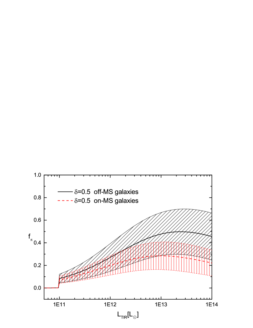
Figure 1.— The pion-production efficiency $f_{\pi}$ for CRs producing 1 PeV neutrinos in star-forming galaxies with different total IR luminosities (assuming the source is at the redshift $z=1$). The shaded regions denote the uncertainties of $f_{\pi}$ resulted from the uncertainties in the galaxy properties (see the text for details).

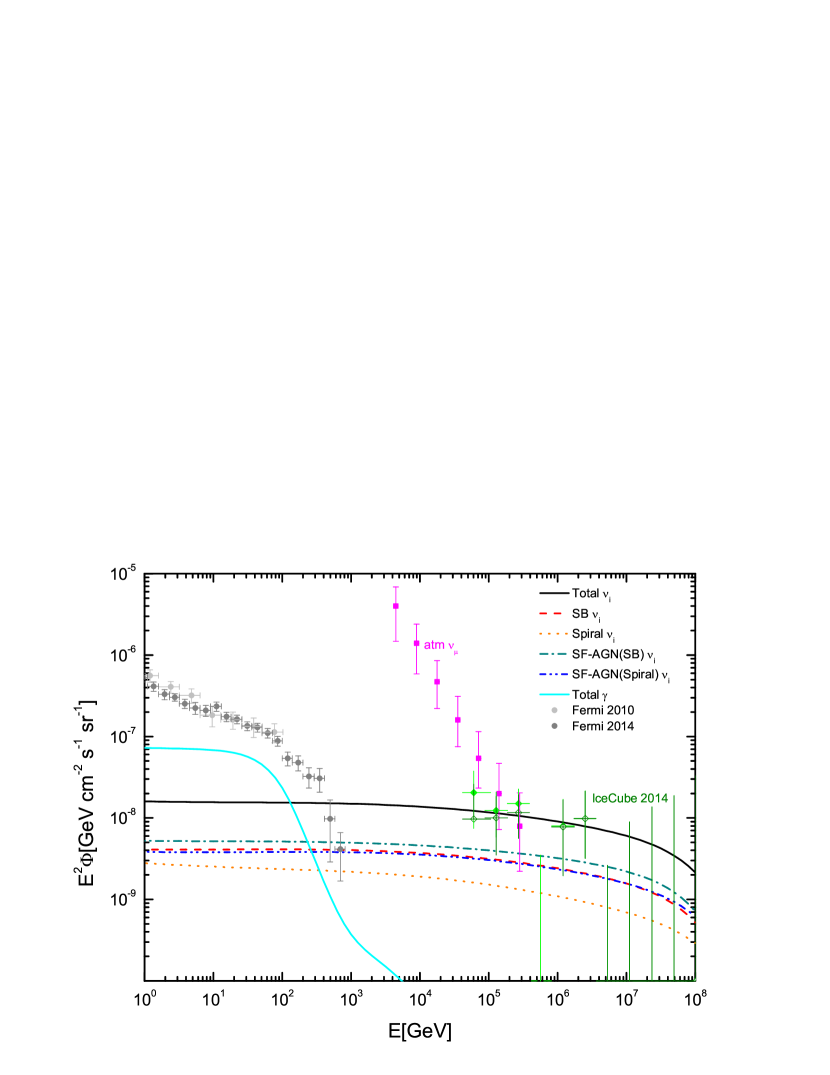
Figure 2.— Accumulated neutrino flux produced by star-forming galaxies of different populations. $D_{0,\text{H}}=10^{27.2}$cm²s^-1, $D_{0,\text{L}}=10^{28}$cm²s^-1 and $\delta=1/3$ are used in the calculation. The red, orange, green, blue lines show the flux contributed by starburst galaxies, normal spiral galaxies, SF-AGNs (SB) and SF-AGNs (spiral), respectively. And the black line shows the sum of them. The cyan line shows the diffuse gamma-ray flux accompanying with the neutrino flux. The extragalactic gamma-ray background data from Fermi/LAT are depicted as the grey dots. The atmospheric neutrino data and the IceCube data are also shown.

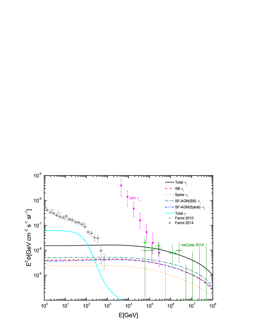
Figure 3.— Same as Figure 2, but with $\delta=0.5$, $D_{0,\text{H}}=10^{26}$cm²s^-1, and $D_{0,\text{L}}=10^{28}$cm²s^-1.

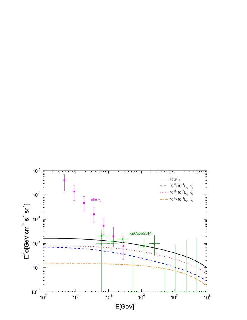
Figure 4.— Accumulated neutrinos flux from star-forming galaxies of different IR luminosities.

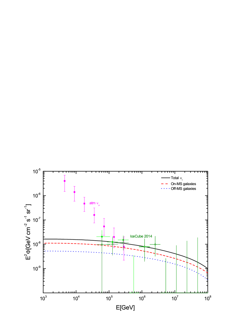
Figure 5.— The same as Figure 3, but the contribution of the galaxies is divided into two subclasses, on-MS galaxies and off-MS galaxies. The black line shows the total flux, while the red and blue lines show the flux contributed by off-MS and on-MS galaxies, respectively.

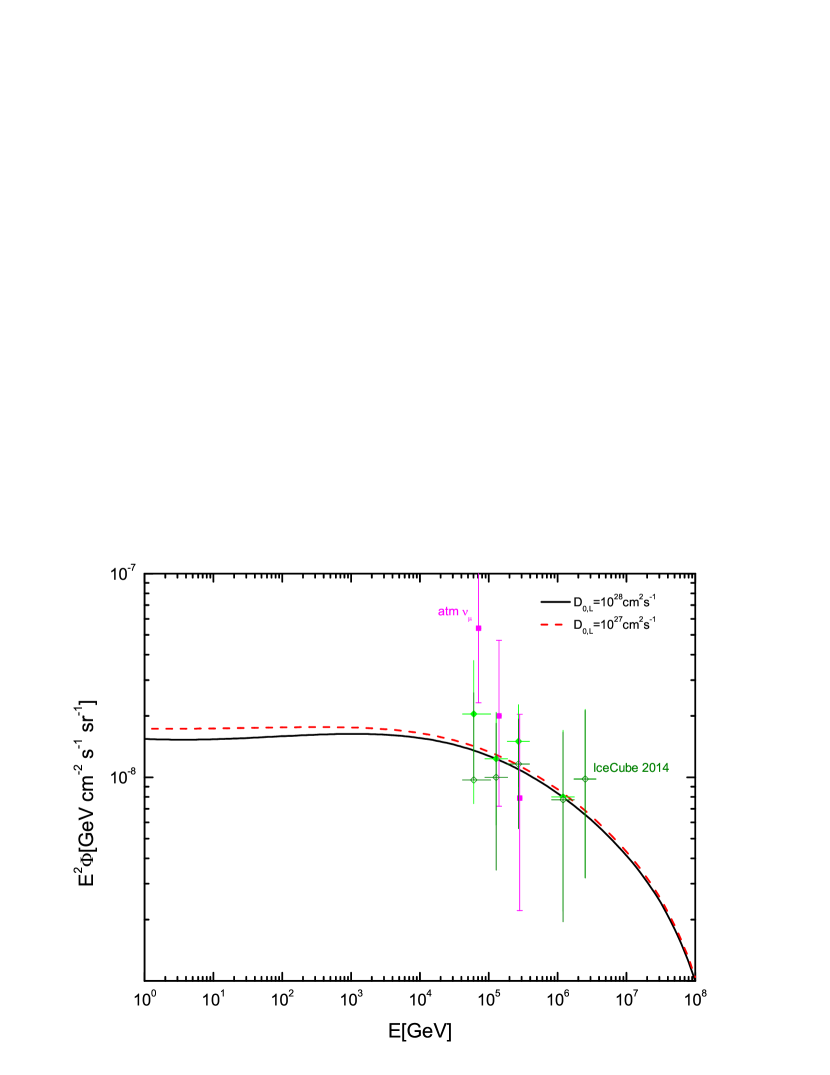
Figure 6.— The accumulated neutrino flux of star-forming galaxies with different values of $D_{0,\text{L}}$, while the other parameters remain unchanged. The black and red lines shows the cases with $D_{0,\text{L}}=10^{28}$cm²s^-1 and $D_{0,\text{L}}=10^{27}$cm²s^-1, respectively.

References

- Aartsen et al. (2014) Aartsen, M. G., Ackermann, M., Adams, J., et al. 2014, Physical Review Letters, 113, 101101
- Abu-Zayyad et al. (2015) Abu-Zayyad, T., Aida, R., Allen, M., et al. 2015, Astroparticle Physics, 61, 93
- Ackermann et al. (2012) Ackermann, M., Ajello, M., Allafort, A., et al. 2012, ApJ, 755, 164
- Ahlers & Murase (2014) Ahlers, M., & Murase, K. 2014, Phys. Rev. D, 90, 023010
- Anchordoqui et al. (2008) Anchordoqui, L. A., Hooper, D., Sarkar, S., & Taylor, A. M. 2008, Astroparticle Physics, 29, 1
- Anchordoqui et al. (2014a) Anchordoqui, L. A., Goldberg, H., Lynch, M. H., et al. 2014, Phys. Rev. D, 89, 083003
- Anchordoqui et al. (2014b) Anchordoqui, L. A., Paul, T. C., da Silva, L. H. M., Torres, D. F., & Vlcek, B. J. 2014, Phys. Rev. D, 89, 127304
- Berezinsky et al. (2006) Berezinsky,V. Gazizov, A. and Grigorieva S., 2006, Phys. Rev. D 74, 043005.
- Bernet et al. (2013) Bernet, M. L., Miniati, F., & Lilly, S. J. 2013, ApJ, 772, LL28
- Bouché et al. (2010) Bouché, N., Dekel, A., Genzel, R., et al. 2010, ApJ, 718, 1001
- Budnik et al. (2008) Budnik, Ran; Katz, Boaz; MacFadyen, Andrew; Waxman, Eli, 2008, ApJ, 673, 928
- Cebrián & Trujillo (2014) Cebrián, M., & Trujillo, I. 2014, MNRAS, 444, 682
- Chabrier (2003) Chabrier, G. 2003, PASP, 115, 763
- Chakraborti et al. (2011) Chakraborti, S.; Ray, A.; Soderberg, A. M.; Loeb, A.; Chandra, 2011, Nature Communications, Volume 2, id. 175
- Chang & Wang (2014) Chang, X.-C., & Wang, X.-Y. 2014, ApJ, 793, 131
- Chiavassa et al. (2014) Chiavassa, A., Apel, W. D., Arteaga-Velázquez, J. C., et al. 2014, Journal of Physics Conference Series, 531, 012001
- Cholis & Hooper (2013) Cholis, I., & Hooper, D. 2013, JCAP, 6, 030
- Daddi et al. (2007) Daddi, E., Dickinson, M., Morrison, G., et al. 2007, ApJ, 670, 156
- Dermer et al. (2014) Dermer, C. D., Murase, K., Inoue, Y. 2014, arXiv:1406.2633
- Dutton et al. (2011) Dutton, A. A., van den Bosch, F. C., Faber, S. M., et al. 2011, MNRAS, 410, 1660
- Elbaz et al. (2007) Elbaz, D., Daddi, E., Le Borgne, D., et al. 2007, A&A, 468, 33
- Engelmann et al. (1990) Engelmann, J. J., Ferrando, P., Soutoul, A., Goret, P., & Juliusson, E. 1990, A&A, 233, 96
- Fang et al. (2014) Fang, K., Kotera, K., Murase, K., & Olinto, A. V. 2014, Phys. Rev. D, 90, 103005
- Fox et al. (2013) Fox, D. B., Kashiyama, K., & Mészarós, P. 2013, ApJ, 774, 74
- Genzel et al. (2010) Genzel, R., Tacconi, L. J., Gracia-Carpio, J., et al. 2010, MNRAS, 407, 2091
- Gruppioni et al. (2013) Gruppioni, C., Pozzi, F., Rodighiero, G., et al. 2013, MNRAS, 432, 23
- He et al. (2013) He, H.-N.; Wang, T.; Fan, Y.-Z.; Liu, S.-M.; Wei, D.-M., Phys. Rev. D, 87, 063011
- Heckman et al. (1990) Heckman, T. M., Armus, L., & Miley, G. K. 1990, ApJS, 74, 833
- High Resolution Fly’S Eye Collaboration et al. (2009) High Resolution Fly’S Eye Collaboration, Abbasi, R. U., Abu-Zayyad, T., et al. 2009, Astroparticle Physics, 32, 53
- Kalashev et al. (2013) Kalashev,O. E., Kusenko, A. and Essey,W., 2013, Phys. Rev. Lett., 111, 041103
- Katz et al. (2009) Katz, B.; Budnik, R.; Waxman, E., 2009, JCAP, id. 020
- Kelner et al. (2006) Kelner, S. R., Aharonian, F. A., & Bugayov, V. V. 2006, Phys. Rev. D, 74, 034018
- Kennicutt (1998) Kennicutt, R. C., Jr. 1998, ApJ, 498, 541
- Kravtsov (2013) Kravtsov, A. V. 2013, ApJ, 764, LL31
- Lacki & Thompson (2010) Lacki, B. C., & Thompson, T. A. 2010, ApJ, 717, 196
- Law et al. (2012) Law, D. R., Steidel, C. C., Shapley, A. E., et al. 2012, ApJ, 745, 85
- Liu & Wang (2012) Liu, R.-Y., Wang, X.-Y., 2012, ApJ, 746, 40
- Liu & Wang (2013) Liu, R.-Y., Wang, X.-Y., 2013, ApJ, 766, 73
- Liu et al. (2014) Liu, R.-Y., Wang, X.-Y., Inoue, S., Crocker, R., & Aharonian, F. 2014, Phys. Rev. D, 89, 083004
- Loeb & Waxman (2006) Loeb, A., & Waxman, E. 2006, JCAP, 5, 3
- Lunardini et al. (2014) Lunardini, C., Razzaque, S., Theodoseau, K. T., & Yang, L. 2014, Phys. Rev. D, 90, 023016
- Martin (2005) Martin, C. L. 2005, ApJ, 621, 227
- Mosleh et al. (2011) Mosleh, M., Williams, R. J., Franx, M., & Kriek, M. 2011, ApJ, 727, 5
- Murase et al. (2013) Murase, K., Ahlers, M., & Lacki, B. C. 2013, Phys. Rev. D, 88, 121301
- Murase & Ioka (2013) Murase, K., & Ioka, K. 2013, Physical Review Letters, 111, 121102
- Neronov et al. (2014) Neronov, A., Semikoz, D., & Tchernin, C. 2014, Phys. Rev. D, 89, 103002
- Peng et al. (2010) Peng, Y.-j., Lilly, S. J., Kovač, K., et al. 2010, ApJ, 721, 193
- Peng et al. (2012) Peng, Y.-j., Lilly, S. J., Renzini, A., & Carollo, M. 2012, ApJ, 757, 4
- Pesce (2012) Pesce, R. 2012, Nuclear Instruments and Methods in Physics Research A, 692, 83
- Pettini et al. (2001) Pettini, M., Shapley, A. E., Steidel, C. C., et al. 2001, ApJ, 554, 981
- Razzaque (2013) Razzaque, S. 2013, Phys. Rev. D, 88, 081302
- Rodighiero et al. (2010) Rodighiero, G., Cimatti, A., Gruppioni, C., et al. 2010, A&A, 518, LL25
- Shapley et al. (2003) Shapley, A. E., Steidel, C. C., Pettini, M., & Adelberger, K. L. 2003, ApJ, 588, 65
- Shen et al. (2003) Shen, S., Mo, H. J., White, S. D. M., et al. 2003, MNRAS, 343, 978
- Stecker (2013) Stecker, F. W., 2013, Phys. Rev. D88, 047301
- Tamborra et al. (2014) Tamborra, I., Ando, S., & Murase, K. 2014, JCAP, 9, 043
- Tang et al. (2014) Tang, Q. W, Wang, X. Y., Tam, T., 2014, ApJ, 794, 26
- The Fermi LAT collaboration et al. (2014) The Fermi LAT collaboration, Ackermann, M., Ajello, M., et al. 2014, arXiv:1410.3696
- Thompson et al. (2006) Thompson, T. A., Quataert, E., Waxman, E., Murray, N., & Martin, C. L. 2006, ApJ, 645, 186
- Wang et al. (2007) Wang, X.-Y., Razzaque, S., Mészáros, P., & Dai, Z.-G. 2007, Phys. Rev. D, 76, 083009
- Wang et al. (2014) Wang, B., Zhao, X. H. & Li, Z., 2014, JCAP, 11, 028
- Waxman & Bahcall (1997) Waxman, E., & Bahcall, J. 1997, Physical Review Letters, 78, 2292
- Webber et al. (2003) Webber, W. R., McDonald, F. B., & Lukasiak, A. 2003, ApJ, 599, 582
- Weiner et al. (2009) Weiner, B. J., Coil, A. L., Prochaska, J. X., et al. 2009, ApJ, 692, 187
- Winter (2014) Winter, W., 2014, Physical Review D, 90, 103003