The effects of deformation parameter on thermal width of moving quarkonia in plasma

Abstract

In general we can say that the thermal width of quarkonia corresponds to imaginary part of it’s potential. Gravity dual of theories give explicit form of potential as $V_{Q\bar{Q}}$. Since there is an explicit formula for $ImV_{Q\bar{Q}}$ one can consider different gravity duals and study the results of contribution of various parameters. Variable gravity duals of moving pair in plasma have different results for potential. Our paper shows that deformation parameter $c$ in warp factor leads to new results that we present them for arbitrary angles of the pair with respect to it’s velocity. We compare our results with the case that no deformation parameter is in metric background. We will see that the thermal width of the pair increases with increasing deformation parameter. Also, for nonzero values of deformation parameter the pair feels moving plasma in all distances. In addition our results indicate that contribution of deformation parameter leads to larger dissociation length for the moving pair reverse to the effect of the pair’s velocity in the plasma.

1 Introduction

When we want to study $Q\bar{Q}$ interaction we should consider the effect of the medium in motion of $Q\bar{Q}$ , because this pair is not produced at rest in QGP. So, the velocity of the pair through the plasma has some effects on its interactions that should be taken into account. The interaction energy has a finite imaginary part at finite temperature that can be used to estimate the thermal width of the quarkonia nbma ; ybm . Calculations of Im$V_{Q\bar{Q}}$ relevant to QCD and heavy ion collisions were performed for static $Q\bar{Q}$ pairs using pQCD mlop and lattice QCD arth ; gaca ; gcs before AdS/CFT.
The AdS/CFT is a correspondence jmm ; ssg ; ew ; oas between a string theory in AdS space and a conformal field theory in physical space-time. It leads to an analytic semi-classical model for strongly coupled QCD. It has scale invariance, dimensional counting at short distances and color confinement at large distances. This theory describes the phenomenology of hadronic properties and demonstrate their ability to incorporate such essential properties of QCD as confinement and chiral symmetry breaking. In the AdS/CFT point of view the $AdS_{5}$ plays important role in describing QCD phenomena. So in order to describe a confining theory, the conformal invariance of $AdS_{5}$ must be broken somehow. Two strategies AdS/QCD background have been suggested in the literatures hard-wall model jee ; hrg ; hr ; eka ; jp ; ldr and soft-wall model ake ; sjb ; gfde ; wdp ; hfm ; wde ; bge ; jni ; hrgr ; hfo ; hjk ; pcf ; ave ; aeg ; aga ; gfd ; zab ; tbt ; avi . In hard-wall model to impose confinement and discrete normalizable modes that is to truncate the regime where string modes can propagate by introducing an IR cutoff in the fifth dimension at a finite value $z_{0}\sim\frac{1}{\Lambda_{QCD}}$. Thus, the hard-wall at $z_{0}$ breaks conformal invariance and allows the introduction of the QCD scale and a spectrum of particle states, they have phenomenological problems, since the obtained spectra does not have Regge behavior. To remedy this it is necessary to introduce a soft cut off, using a dilaton field or using a warp factor in the metric jee ; wde . These models are called soft wall models. The soft-wall and hard-wall approach has been successfully applied to the description of the mass spectrum of mesons and baryons, the pion leptonic constant, the electromagnetic form factors of pion and nucleons, etc. On the other hand the study of the moving heavy quarkonia in space-time with AdS/QCD approach plays important role in interaction energy mst ; msd ; mmk ; gac . By using different metric backgrounds we see different effects on interaction energy.
Evaluation of Im$V_{Q\bar{Q}}$ will yield to determine the suppression of ${Q\bar{Q}}$ in heavy ion collisionsif . The main idea is using boosted frame to have Re $V_{Q\bar{Q}}$ and Im $V_{Q\bar{Q}}$ fn for ${Q\bar{Q}}$ in a plasma.
From viewpoint of holography, the AdS/CFT correspondence can describe a “brocken conformal symmetry”, when one adds a proper deformed warp factor in front of the $AdS_{5}$ metric structure jer ; gfdt ; jba ; mkr ; tsss ; tsa ; shm ; akek ; oan ; fzu ; gfdet ; jpsh ; kghm ; kghn ; ccm ; ugek ; uek ; dfze ; hjp ; shem ; dlis . So, $e^{cz^{2}}$ is a positive quadratic correction with z, the fifth dimension.
One natural question is about the connection between the warp factor and the potential $V_{Q\bar{Q}}$. In this work, the procedure of sif is followed to evaluate the imaginary part of potential for an AdS metric background with deformation parameter in warp factor. It is interesting to see “ what will happen if meson be in a deformed AdS?”
It is a trend to see the effects of deformation parameter on Re$V_{Q\bar{Q}}$ and Im$V_{Q\bar{Q}}$ which are evidences for “usual” or “unusual" behavior of meson in compare with the $c=0$ case. As expected in the limit of $c\rightarrow 0$, all results are equal to the results of $AdS_{5}$ case. All above informations give us motivation to work on effect of the deformation parameter in $AdS$ metric background on real and imaginary parts of potential. So, we organized the paper as follows. In section 2, we discuss the case where the pair is moving perpendicularly to the joining axis of the dipole in deformed AdS, we assume this metric background for ${Q\bar{Q}}$ and find some relations for real and imaginary parts of potential. This example will be presented with some numerical results for different values of deformation parameter. Then we consider general orientation of ${Q\bar{Q}}$ in section 3 and follow the procedure as before. Section 4 would be our conclusion and some suggestions for future work.

2 ${Q\bar{Q}}$ in an deformed AdS, perpendicular case

In this section we consider soft-wall metric background with deformation parameter in warp factor at finite temperature case. So, we present general relations for real and imaginary parts of potential when the dipole is moving with velocity $\eta$ perpendicularly to the wind sif .
In our case we apply the general result for deformed AdS, the dual gravity metric will be as:

$$ds^{2}=e^{2A(z)}[-f(z)dt^{2}+\Sigma_{i=1}^{i=3}dx^{2}+\frac{1}{f(z)}dz^{2}],$$ (1)

Where $A(z)=-\ln\frac{z}{R}+\frac{1}{4}cz^{2}$ and $f(z)=1-(\frac{z}{z_{h}})^{4}$. As mentioned before $c$ is deformation parameter and $R$ is the AdS curvature radius, also $0\leq z\leq z_{h}$, $z_{h}=\frac{1}{\pi T}$ and $T$ is boundary field theory’s temperature. We have a dynamic dilaton in action for the background and we write our calculations in string frame. If dilaton is such that it enters directly in the worldsheet action in the form $\phi R$. May be our concern is about the effect of a nontrivial dilaton profile to the string action. But somewhen people neglect it at the first step ugkm and leave it for future study. Then one can check that the integral on the action correspond to worldsheet with higher genus. This means that we are doing string interactions and going to higher order in string perturbation theory. But now, for leading order calculations in genus, we need not to bother with this term even if the geometry has a dynamical dilaton. On the other hand one trace of dynamical dilaton can appear via temperature if we want to calculate it with GSH approach. So, the exact temperature will be in hand. But we refer the reader to dlis for the reasons that in deformed AdS model with quadratic correction in warp factor the “temperature” takes the form of AdS-SW BH temperature. So, we have a deformed AdS which in the limit $c\rightarrow 0$ becomes $AdS_{5}$. This comparing results help us to underestand the effects of deformation parameter on the physical quantities such as interaction energy. Our calculations in the cases of $LT$, $ReV_{Q\bar{Q}}$ and $ImV_{Q\bar{Q}}$ give us motivation to compare results between different values of deformation parameter.
From metric background (2.1) one can obtain:

$$G_{00}=\frac{R^{2}}{z^{2}}[1-(\frac{z}{z_{h}})^{4}]e^{\frac{cz^{2}}{2}}$$ (2)

$$G_{xx}=\frac{R^{2}}{z^{2}}e^{\frac{cz^{2}}{2}}$$ (3)

$$G_{zz}=\frac{R^{2}}{z^{2}}[1-(\frac{z}{z_{h}})^{4}]^{-1}e^{\frac{cz^{2}}{2}},$$ (4)

with these definitions,

$$\tilde{M}(z)\equiv M(z)\cosh^{2}\eta-N(z)\sinh^{2}\eta\$$ (5)

$$\tilde{V}(z)\equiv V(z)\cosh^{2}\eta-P(z)\sinh^{2}\eta\$$ (6)

$$M(z)\equiv G_{00}G_{zz}$$ (7)

$$V(z)\equiv G_{00}G_{xx}$$ (8)

$$P(z)\equiv{G_{xx}}^{2}$$ (9)

$$N(z)\equiv G_{xx}G_{zz},$$ (10)

we continue with hamiltonian,

$$H(z)\equiv\sqrt{\frac{\tilde{V}(z)}{\tilde{V}_{\ast}}\frac{\tilde{V}(z)-\tilde{V}_{\ast}}{\tilde{M}(z)}},$$ (11)

where $\tilde{V}_{\ast}$ means $\tilde{V}(z_{\ast})$ and $\ast$ is the deepest position of the string in the bulk.
The equation of motion and the boundary conditions of the string relates $L$(length of the line joining both quarks) with $z_{\ast}$ as follows,

$$\frac{L}{2}=\int_{r_{\ast}}^{\Lambda}\frac{dr}{H(r)}.$$ (12)

So, for the corresponding case we have,

$$\frac{L}{2}=-\int_{0}^{z_{\ast}}\frac{dz}{H(z)}.$$ (13)

In order to relation between $S_{str}$ and $z_{\ast}$ we find the regularized integral fn as,

$$S_{str}^{reg} = \frac{T}{\pi\alpha^{\prime}}\int_{r_{*}}^{\infty}dr\,\left[\sqrt{\tilde{M}(r)}\sqrt{\frac{\tilde{V}(r)}{\tilde{V}(r_{*})}}\left(\frac{\tilde{V}(r)}{\tilde{V}(r_{*})}-1\right)^{-1/2}-\sqrt{M_{0}(r)}\right]$$ (14)

$$- \frac{T}{\pi\alpha^{\prime}}\int_{r_{h}}^{r_{*}}dr\,\sqrt{M_{0}(r)},$$

and we obtain the following results

$$LT=\frac{2}{\pi}y_{h}\sqrt{1-y_{h}^{4}\cosh^{2}\eta}\int_{1}^{\infty}\frac{dy}{\sqrt{(y^{4}-y_{h}^{4})[e^{\frac{cy_{h}^{2}}{\pi^{2}T^{2}}(\frac{1}{y^{2}}-1)}(y^{4}-y_{h}^{4}\cosh^{2}\eta)-(1-y_{h}^{4}\cosh^{2}\eta)]}}$$ (15)

where   $y=\frac{z_{\ast}}{z}$   and  $y_{h}=\frac{z_{\ast}}{z_{h}}$

$$S_{str}^{reg} = T^{2}\frac{\sqrt{\lambda}}{y_{h}}\{\int_{1}^{\infty}dy[\frac{e^{\frac{cy_{h}^{2}}{\pi^{2}T^{2}}(\frac{1}{y^{2}}-\frac{1}{2})}(y^{4}-y_{h}^{4}\cosh^{2}\eta)}{\sqrt{(y^{4}-y_{h}^{4})[e^{\frac{cy_{h}^{2}}{\pi^{2}T^{2}}(\frac{1}{y^{2}}-1)}(y^{4}-y_{h}^{4}\cosh^{2}\eta)-(1-y_{h}^{4}\cosh^{2}\eta)]}}$$ (16)

$$- e^{\frac{cy_{h}^{2}}{\pi^{2}T^{2}y^{2}}}]-\int_{0}^{1}dy\quad e^{\frac{cy_{h}^{2}}{\pi^{2}T^{2}y^{2}}}\},$$

Where $\lambda=\frac{R^{4}}{\alpha^{2}\prime}$ is and $\alpha^{\prime}$ is the ’t Hooft coupling of the gauge theory. Finally, we find the real part of potential as
$ReV_{Q\bar{Q}}=\frac{S_{str}^{reg}}{T}$.
Now we present a derivation of relation for imaginary part of potential from fn . The reader can see more details in that reference. From there we can say one should consider the effect of worldsheet fluctuations around the classical configuration $z_{c}(x)$,

$$z(x)=z_{c}(x)\rightarrow z(x)=z_{c}(x)+\delta z(x).$$ (17)

And then the fluctuations should be taken into account in partition function so one arrives at,

$$Z_{str}\sim\int\mathcal{D}\delta z(x)e^{iS_{NG}(z_{c}(x)+\delta z(x))}.$$ (18)

Then there is an imaginary part of potential in action so , by dividing the interval region of x into $2N$ points where $N\longrightarrow\infty$ that should be taken into account at the end of calculation we arrive at,

$$Z_{str}\sim\lim_{N\to\infty}\int d[\delta z(x_{-N})]\ldots d[\delta z(x_{N})]\exp{\left[i\frac{\mathcal{T}\Delta x}{2\pi\alpha^{\prime}}\sum_{j}\sqrt{M(z_{j})(z^{\prime}_{j})^{2}+V(z_{j})}\right]}.$$ (19)

Notice that we should expand $z_{c}(x_{j})$ around $x=0$ and keep only terms up to second order of it because thermal fluctuations are important around $z_{\ast}$ which means $x=0$,

$$z_{c}(x_{j})\approx z_{\ast}+\frac{x_{j}^{2}}{2}z_{c}^{\prime\prime}(0),$$ (20)

With considering small fluctuations finally we will have,

$$V(z_{j})\approx V_{*}+\delta zV^{\prime}_{*}+z_{c}^{\prime\prime}(0)V^{\prime}_{*}\frac{x_{j}^{2}}{2}+\frac{\delta z^{2}}{2}V^{\prime\prime}_{*},$$ (21)

where $V_{\ast}\equiv V(z_{\ast})$ and $V^{\prime}_{\ast}\equiv V^{\prime}(z_{\ast})$. With (2.20), (2.21) and (2.19) one can derive (2.22), (2.23) and (2.24),

$$S^{NG}_{j}=\frac{\mathcal{T}\Delta x}{2\pi\alpha^{\prime}}\sqrt{C_{1}x_{j}^{2}+C_{2}}$$ (22)

$$C_{1}=\frac{z_{c}^{\prime\prime}(0)}{2}\left[2M_{*}z_{c}^{\prime\prime}(0)+V_{*}^{\prime}\right]$$ (23)

$$C_{2}=V_{*}+\delta zV^{\prime}_{*}+\frac{\delta z^{2}}{2}V^{\prime\prime}_{*}.$$ (24)

For having $ImV_{Q\bar{Q}}\neq 0$ the function in the square root of (2.22) should be negative. then, we consider j-th contribution to $Z_{str}$ as,

$$I_{j}\equiv\int\limits_{\delta z_{jmin}}^{\delta z_{jmax}}d(\delta z_{j})\,\exp{\left[i\frac{\mathcal{T}\Delta x}{2\pi\alpha^{\prime}}\sqrt{C_{1}x_{j}^{2}+C_{2}}\right]},$$ (25)

For every $\delta z$ between minimum and maximum of it’s values which are the roots of $C_{1}x_{j}^{2}+C_{2}$ in $\delta z$, one leads to $C_{1}x_{j}^{2}+C_{2}<0$. The extermal value of the function

$$D(\delta z_{j})\equiv C_{1}x_{j}^{2}+C_{2}(\delta z_{j})$$ (26)

is,

$$\delta z=-\frac{V^{\prime}_{*}}{V^{\prime\prime}_{*}}.$$ (27)

So, $D(\delta z_{j})<0\longrightarrow-x_{c}<x_{j}<x_{c}$ leads us to have an imaginary part in square root, where,

$$x_{c}=\sqrt{\frac{1}{C_{1}}\left[\frac{V^{\prime 2}_{*}}{2V^{\prime\prime}_{*}}-V_{*}\right]}.$$ (28)

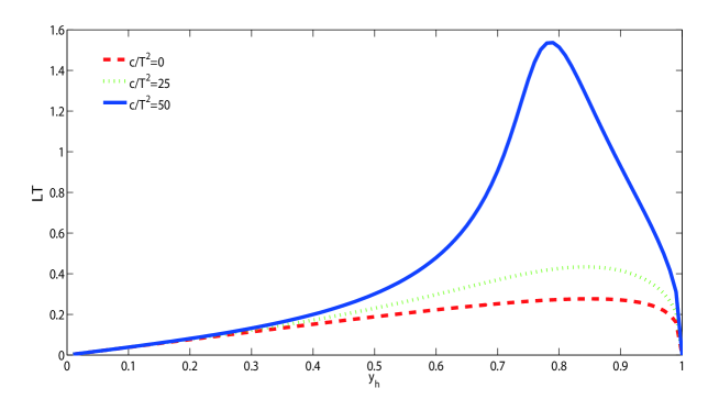
Figure 1: $LT$ as a function of $y_{h}$ at $\eta=0$. $Q\bar{Q}$ is oriented to the hot wind and different values of deformation parameter are contributed. The solid blue curve corresponds to $\frac{c}{T^{2}}=50$, the dotted green curve to $\frac{c}{T^{2}}=25$ and the dashed red curve to $\frac{c}{T^{2}}=0$

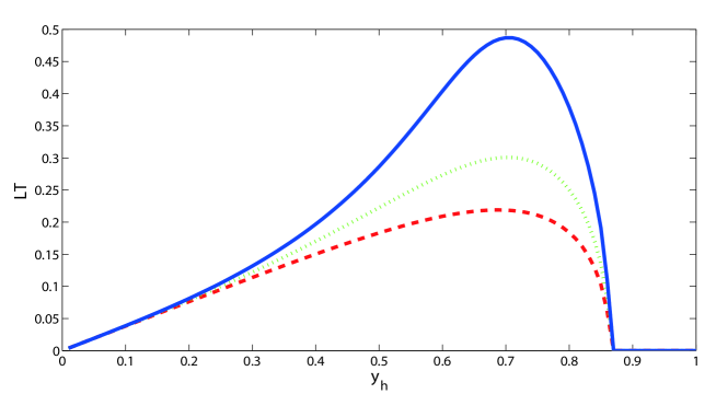
Figure 2: $LT$ as a function of $y_{h}$ at $\eta=0.8$. $Q\bar{Q}$ is oriented to the hot wind and different values of deformation parameter are contributed. The solid blue curve corresponds to $\frac{c}{T^{2}}=50$, the dotted green curve to $\frac{c}{T^{2}}=25$ and the dashed red curve to $\frac{c}{T^{2}}=0$

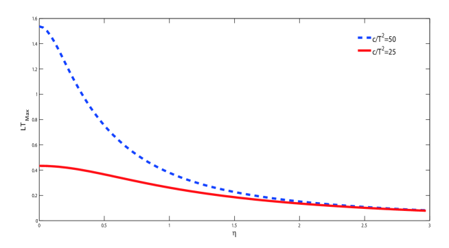
Figure 3: $LT_{max}$ as a function of $\eta$. $Q\bar{Q}$ is oriented to the hot wind and different values of deformation parameter are contributed. The dashed blue curve corresponds to $\frac{c}{T^{2}}=50$ and the solid red curve to $\frac{c}{T^{2}}=25$.

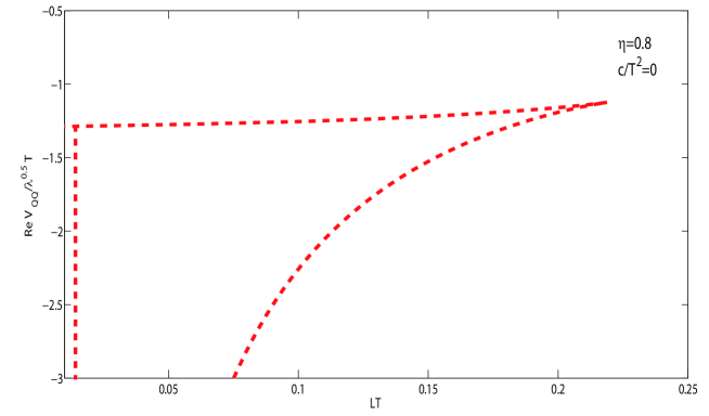
Figure 4: $ReV_{Q\bar{Q}}$ as a function of $LT$ at a fixed velocity $\eta=0.8$ the pair is oriented to the hot wind and and deformation parameter is zero

Figure 5: $ReV_{Q\bar{Q}}$ as a function of $LT$ at a fixed velocity $\eta=0.8$ the pair is oriented to the hot wind and scaled deformation parameter is 25

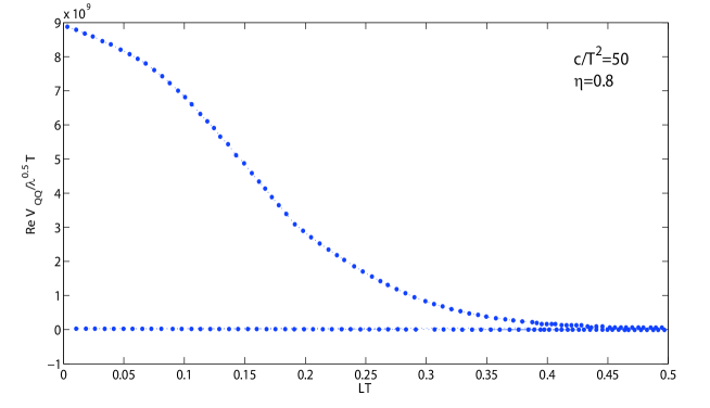
Figure 6: $ReV_{Q\bar{Q}}$ as a function of $LT$ at a fixed velocity $\eta=0.8$ the pair is oriented to the hot wind and scaled deformation parameter is 50

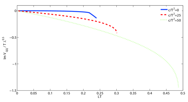
Figure 7: Imaginary part of potential as a function of $LT$, at a fixed velocity $\eta=0.4$. The pair is oriented to the hot wind and different values of scaled deformation parameter are contributed. The solid blue curve corresponds to $\frac{c}{T^{2}}=0$ , the dashed red curve to $\frac{c}{T^{2}}=25$ and the dotted green curve to $\frac{c}{T^{2}}=50$.

If the square root in (2.28) is not real we should take $x_{c}=0$. After all these conditions we can approximate $D(\delta z)$ by $D(-\frac{V^{\prime}_{\ast}}{V"_{\ast}})$ in $I_{j}$,

$$I_{j}\sim\exp\left[i\frac{\mathcal{T}\Delta x}{2\pi\alpha^{\prime}}\sqrt{C_{1}x_{j}^{2}+V_{*}-\frac{V^{\prime 2}_{*}}{2V^{\prime\prime}_{*}}}\right].$$ (29)

The total contribution to the imaginary part, will be in hand with continuum limit. So,

$$\mathrm{Im}\,V_{Q\bar{Q}}=-\frac{1}{2\pi\alpha^{\prime}}\int\limits_{|x|<x_{c}}dx\sqrt{-x^{2}C_{1}-V_{*}+\frac{V^{\prime 2}_{*}}{2V^{\prime\prime}_{*}}}\,.$$ (30)

And finally after evaluating the integral one can arrive at the expression for imaginary part of potential as,

$$\mathrm{Im}\,V_{Q\bar{Q}}=-\frac{1}{2\sqrt{2}\alpha^{\prime}}\sqrt{M_{*}}\left[\frac{V^{\prime}_{*}}{2V^{\prime\prime}_{*}}-\frac{V_{*}}{V^{\prime}_{*}}\right].$$ (31)

Now, we are ready to calculate the imaginary part of potential in case of $\tilde{M}_{\ast}>0$ so according to (2.31) and with our deformed AdS metric (2.1) we have following relation,

$$\frac{ImV_{Q\bar{Q}}}{\sqrt{\lambda}} = -\frac{\pi T}{4\sqrt{2}y_{h}}e^{\frac{cy_{h}^{2}}{2\pi^{2}T^{2}}}\sqrt{\frac{1-y_{h}^{4}\cosh^{2}\eta}{1-y_{h}^{4}}}$$ (32)

$$\times [\frac{\frac{2cy_{h}^{2}}{\pi^{2}T^{2}}(1-y_{h}^{4}\cosh^{2}\eta)+4}{\frac{cy_{h}^{2}}{\pi^{2}T^{2}}(2-10y_{h}^{4}\cosh^{2}\eta)+12}-\frac{(1-y_{h}^{4}\cosh^{2}\eta)}{2+\frac{cy_{h}^{2}}{2\pi^{2}T^{2}}(1-y_{h}^{4}\cosh^{2}\eta)}].$$

In Fig.1 and 2 we can see the behavior of $LT$ as a function of $y_{h}$ for different values of deformation parameter for this perpendicular case. As we show the maximum of the $LT(y_{h})$ which is an indicative of the limit of classical gravity calculations, increases with increasing deformation parameter.
On the contrary, increasing velocity reduces $LT_{max}$ , as it is mentioned in Fig.3. Furthermore, increasing deformation parameter increases $LT_{max}$ which has been used to define a dissociation length for the moving $Q\bar{Q}$ pair.
Fig 4,5 and 6 show the behavior of $ReV_{Q\bar{Q}}$ as a function of $LT$. As we know for zero value of c in short distances the pair does not feel the moving plasma and upper branch shows saddle point of string action. In compare with that, when c is nonzero pair can feel moving plasma for all values of distances. In addition , we can see with increasing deformation parameter the real part of potential increases and the unphysical curve corresponds to $q<q_{max}$ and the lower branch is the dominant contribution to the action which corresponds to $q>q_{max}$.
The imaginary part of the potential corresponds to the dissociation properties of heavy quarkonia. In Fig.7 our results indicate that the thermal width of the pair increases with increasing the deformation parameter at a fixed velocity.

3 ${Q\bar{Q}}$ in an deformed AdS at arbitrary angles

In this section we extend our calculations for arbitrary angles, it means that orientation of dipole can have any arbitrary angle with respect to velocity vector. As before we extract the real and imaginary parts of potential with method of sif , $\theta$ is the angle of the dipole with respect to the $X_{d-1}$ and dipole is on the $(X_{1},X_{d-1})$ plane. The boundary conditions are,

$$z\left(\pm\frac{L}{2}\sin\theta\right) =0$$

$$X_{d}\left(\pm\frac{L}{2}\sin\theta\right) =\pm\frac{L}{2}\cos\theta$$ (33)

And the action is,

$$S_{str}=-\frac{\mathcal{T}}{2\pi\alpha^{\prime}}\int d\sigma\mathcal{L},$$ (34)

where the lagrangian is defined as,

$$\mathcal{L}\equiv\sqrt{\left[M(z)\cosh^{2}\eta-N(z)\sinh^{2}\eta\right]z^{\prime}(\sigma)^{2}+V(z)X_{d}^{\prime}(\sigma)^{2}+\left[V(z)\cosh^{2}\eta-P(z)\sinh^{2}\eta\right]}.$$ (35)

There are two constants of motion which are,

$$\mathcal{H}\equiv Q\equiv\mathcal{L}-\frac{dz}{d\sigma}\frac{\partial\mathcal{L}}{\partial z^{\prime}}-\frac{dX_{d}}{d\sigma}\frac{\partial\mathcal{L}}{\partial X_{d}^{\prime}}$$ (36)

$$K\equiv\frac{\partial\mathcal{L}}{\partial X_{d}^{\prime}},$$ (37)

with (3.3), (3.4) and (3.5) after some algebra one can arrive at,

$$Q^{2}\left[M(z)\cosh^{2}\eta-N(z)\sinh^{2}\eta\right]z^{\prime}(\sigma)^{2}+Q^{2}V(z)X_{d-1}^{\prime}(\sigma)^{2}+$$

$$+\left[V(z)\cosh^{2}\eta-P(z)\sinh^{2}\eta\right]\left\{Q^{2}-\left[V(z)\cosh^{2}\eta-P(z)\sinh^{2}\eta\right]\right\}=0$$ (38)

$$K^{2}\left[M(z)\cosh^{2}\eta-N(z)\sinh^{2}\eta\right]z^{\prime}(\sigma)^{2}+V(z)(K^{2}-V(z))\,X_{d-1}^{\prime 2}(\sigma)+$$

$$+K^{2}\left[V(z)\cosh^{2}\eta-P(z)\sinh^{2}\eta\right]=0\,.$$ (39)

with inserting ${X^{\prime}_{d}}^{2}$ from (3.6) into (3.7) and doing some manipulations the result is,

$$Q^{2}V(z)\left[M(z)\cosh^{2}\eta-N(z)\sinh^{2}\eta\right]z^{\prime}(\sigma)^{2}=$$

$$=(V(z)-K^{2})\left[V(z)\cosh^{2}\eta-P(z)\sinh^{2}\eta\right]^{2}-V(z)\left[V(z)\cosh^{2}\eta-P(z)\sinh^{2}\eta\right]Q^{2},$$ (40)

and

$$Q^{2}V^{2}(X_{d-1}^{\prime})^{2}=K^{2}\left[V(z)\cosh^{2}\eta-P(z)\sinh^{2}\eta\right]^{2}.$$ (41)

It is clear that we must have $Z(\sigma=0)=Z_{\ast}$ , $Z^{\prime}(\sigma=0)=0$ and $X_{d}(\sigma=0)=0$ so,

$$(V_{\ast}-K^{2})(V_{\ast}\cosh^{2}\eta-P_{\ast}\sinh^{2}\eta)-V_{\ast}Q^{2}=0.$$ (42)

Proceeding by boundary conditions (3.1) and equations of motion (3.8) and (3.9) we arrive at these two relations,

$$\frac{L}{2}\sin\theta= -Q\int_{0}^{z_{\ast}}\,dz\left\{\frac{V(z)}{V(z)\cosh^{2}\eta-P(z)\sinh^{2}\eta}\right.\times$$

$$\times\left.\frac{M(z)\cosh^{2}\eta-N(z)\sinh^{2}\eta}{\left[(V(z)-K^{2})\left[V(z)\cosh^{2}\eta-P(z)\sinh^{2}\eta\right]-V(z)Q^{2}\right]}\right\}^{-1/2},$$ (43)

$$\frac{L}{2}\cos\theta=-K\int_{0}^{z_{\ast}}\,dz\,\sqrt{\frac{\left[M(z)\cosh^{2}\eta-N(z)\sinh^{2}\eta\right]\left[V(z)\cosh^{2}\eta-P(z)\sinh^{2}\eta\right]}{V(z)\left\{(V(z)-K^{2})\left[V(z)\cosh^{2}\eta-P(z)\sinh^{2}\eta\right]-V(z)Q^{2}\right\}}}.$$ (44)

Finally the action is,

$$S=-\frac{\mathcal{T}}{\pi\alpha^{\prime}}\int_{0}^{z_{\ast}}\,dz\,\sqrt{\frac{V(z)\left[M(z)\cosh^{2}\eta-N(z)\sinh^{2}\eta\right]\left[V(z)\cosh^{2}\eta-P(z)\sinh^{2}\eta\right]}{\left\{(V(z)-K^{2})\left[V(z)\cosh^{2}\eta-P(z)\sinh^{2}\eta\right]-V(z)Q^{2}\right\}}}\,.$$ (45)

After regularizing it we have,

$$S_{reg} =-\frac{\mathcal{T}}{\pi\alpha^{\prime}}\int_{0}^{z_{\ast}}\,dz\,\left\{\sqrt{\frac{V(z)\left[M(z)\cosh^{2}\eta-N(z)\sinh^{2}\eta\right]\left[V(z)\cosh^{2}\eta-P(z)\sinh^{2}\eta\right]}{\left\{(V(z)-K^{2})\left[V(z)\cosh^{2}\eta-P(z)\sinh^{2}\eta\right]-V(z)Q^{2}\right\}}}\right.$$

$$\left.-\sqrt{M_{0}(z)}\right\}-\frac{\mathcal{T}}{\pi\alpha^{\prime}}\int_{z_{h}}^{z_{\ast}}dz\sqrt{M_{0}(z)}.$$ (46)

As before, in the absence of black brane $M(z)$ for $T=0$ leads to $M_{0}$ and $ReV_{Q\bar{Q}}=\frac{S_{str}^{reg}}{T}$. For imaginary part we have two degrees of freedom $Z(\sigma)$ and $X_{d-1}(\sigma)$. The string partition function is,

$$Z_{str}\sim\int D(\delta z)\,D(\delta X_{d-1})e^{iS_{str}(\bar{z}+\delta z,\bar{X}_{d-1}+\delta X_{d})},$$ (47)

where fluctuations $\delta z(\sigma)$ and $\delta X_{d-1}(\sigma)$ are considered with $\frac{\partial z}{\partial\sigma}\longrightarrow 0$ and $\frac{\partial X_{d-1}}{\partial\sigma}\longrightarrow 0$.
As before with action (3.2) and partitioning the interval in $2N$ subintervals we arrive at,

$$Z_{str}\sim\left(\int_{-\infty}^{\infty}d(\delta z_{-N})\,d(\delta X_{{d-1},-N})\right)\cdots\left(\int_{-\infty}^{\infty}d(\delta z_{N})\,d(\delta X_{{d-1},N})\right)e^{i\frac{\mathcal{T}\Delta x}{2\pi\alpha^{\prime}}\mathcal{L}_{j}},$$ (48)

and

$$\mathcal{L}_{j}=\sqrt{\tilde{M}(z(x_{j}))(z^{\prime}(x_{j}))^{2}+V(z(x_{j}))(X_{d-1}^{\prime}(x_{j}))^{2}+\tilde{V}(x_{j})}.$$ (49)

We expand the classical solution $\bar{z}(0)$ around $\sigma=0$ to quadratic order on $\sigma$. If the string did not sag, then we would have $X_{d-1}(\sigma)=\frac{\sigma}{\tan\tilde{\theta}}$ and around $\sigma=0$ we will have,

$$X_{d-1}(\sigma)=\frac{\sigma}{\tan\tilde{\theta}}+b\sigma^{3}+O(\sigma^{5}),$$ (50)

$\tilde{\theta}$ is equal to $\theta$ and b is a constant. Because of the symmetry of the problem under reflections with respect to the origin of the $(X_{1},X_{d})$ plane, $X_{d}(\sigma)$ must be an odd function of $\sigma$ so,

$$X_{d-1}^{\prime}(\sigma)^{2}=\frac{1}{\tan^{2}\tilde{\theta}}+\frac{6b}{\tan\tilde{\theta}}\sigma^{2}.$$ (51)

With inserting (3.19) into (3.17), one can arrive at,

$$\mathcal{L}_{j}=\sqrt{\tilde{C}_{1}x_{j}^{2}+\tilde{C}_{2}},$$ (52)

with these definition,

$$\tilde{C}_{1}\equiv\tilde{M}_{\ast}\bar{z}^{\prime\prime}(0)^{2}+\frac{1}{2}\left(\frac{V^{\prime}_{\ast}}{\tan^{2}\tilde{\theta}}+\tilde{V}^{\prime}_{\ast}\right)\bar{z}^{\prime\prime}(0)+\frac{6b}{\tan\tilde{\theta}}V_{\ast}$$ (53)

$$\tilde{C}_{2}\equiv\left(\frac{V_{\ast}}{\tan^{2}\tilde{\theta}}+\tilde{V}_{\ast}\right)+\left(\frac{V^{\prime}_{\ast}}{\tan^{2}\tilde{\theta}}+\tilde{V^{\prime}}_{\ast}\right)\delta z+\left(\frac{V^{\prime\prime}_{\ast}}{\tan^{2}\tilde{\theta}}+\tilde{V^{\prime\prime}}_{\ast}\right)\frac{(\delta z)^{2}}{2}.$$ (54)

As previous section after some algebric calculations the explicite analytical expression for $ImV_{Q\bar{Q}}$ would be,

$$\mathrm{Im}\,V_{Q\bar{Q}}=-\frac{1}{4\alpha^{\prime}}\frac{1}{\sqrt{\tilde{C}_{1}}}\left[\frac{\left(\frac{V_{\ast}^{\prime}}{\tan^{2}\tilde{\theta}}+\tilde{V}_{\ast}^{\prime}\right)^{2}}{2\left(\frac{V_{\ast}^{\prime\prime}}{\tan^{2}\tilde{\theta}}+\tilde{V}_{\ast}^{\prime\prime}\right)}-\left(\frac{V_{\ast}}{\tan^{2}\tilde{\theta}}+\tilde{V}_{\ast}\right)\right]\,.$$ (55)

Again we emphasis that all above derivations about imaginary and real parts of potential are presented in references that we mentioned before, but we follow them here for convenience of the reader. Now we can come back to our main case and follow it with metric (2.1). With using (3.8) and (3.9) we will have,

$$q^{2}\left(\frac{dy}{d\tilde{\sigma}}\right)^{2}=(y^{4}-\cosh^{2}\eta)((e^{\frac{c}{\pi^{2}T^{2}y^{2}}})(y^{4}-1)-p^{2})-q^{2}(y^{4}-1)\quad\quad\mathrm{and}$$ (56)

$$\left(\frac{d\chi}{d\tilde{\sigma}}\right)^{2}=\frac{p^{2}}{q^{2}}\left(\frac{y^{4}-\cosh^{2}\eta}{y^{4}-1}\right)^{2},$$ (57)

where we defined the dimensionless variables $y\equiv z_{h}/z$, $\chi\equiv X_{d}/z_{h}$ and $\tilde{\sigma}\equiv\sigma/z_{h}$ as well as the dimensionless integration constants $q^{2}\equiv Q^{2}z_{h}^{4}/R^{4}$ and $p^{2}=K^{2}z_{h}^{4}/R^{4}$ also the boundary conditions become,

$$y\left(\pm\pi\frac{LT}{2}\sin\theta\right) =0$$

$$\chi\left(\pm\pi\frac{LT}{2}\sin\theta\right) =\pm\pi\frac{LT}{2}\cos\theta.$$ (58)

So, (3.11), (3.12) and (3.10) lead to (3.27), (3.28) and (3.29),

$$\frac{LT}{2}\pi\sin\theta=q\int_{y_{\ast}}^{\tilde{\Lambda}}\,\frac{dy}{\sqrt{((e^{\frac{c}{\pi^{2}T^{2}y^{2}}})(y^{4}-1)-p^{2})(y^{4}-\cosh^{2}\eta)-q^{2}(y^{4}-1)}}\quad\quad\mathrm{and}$$ (59)

$$\frac{LT}{2}\pi\cos\theta=p\int_{y_{\ast}}^{\tilde{\Lambda}}\,dy\,\frac{y^{4}-\cosh^{2}\eta}{y^{4}-1}\frac{1}{\sqrt{((e^{\frac{c}{\pi^{2}T^{2}y^{2}}})(y^{4}-1)-p^{2})(y^{4}-\cosh^{2}\eta)-q^{2}(y^{4}-1)}}\,.$$ (60)

$$((e^{\frac{c}{\pi^{2}T^{2}y_{\ast}^{2}}})(y_{\ast}^{4}-1)-p^{2})(y_{\ast}^{4}-\cosh^{2}\eta)-q^{2}(y_{\ast}^{4}-1)=0\,.$$ (61)

Therefore the real part of potential is,

$$\frac{\mathrm{Re}\,V_{Q\bar{Q}}}{T\sqrt{\lambda}} = \int_{y_{\ast}}^{\infty}dy\left[\frac{e^{\frac{c}{\pi^{2}T^{2}y^{2}}}(y^{4}-\cosh^{2}\eta)}{\sqrt{(y^{4}-\cosh^{2}\eta)(e^{\frac{c}{\pi^{2}T^{2}y^{2}}}(y^{4}-1)-p^{2})-q^{2}(y^{4}-1)}}-e^{\frac{c}{2\pi^{2}T^{2}y^{2}}}\right]$$ (62)

$$- \int_{0}^{y_{\ast}}dye^{\frac{c}{2\pi^{2}T^{2}y^{2}}}\,.$$

And from (3.23) we arrive at imaginary part of potential as,

$$\frac{\mathrm{Im}\,V_{Q\bar{Q}}}{T\sqrt{\lambda}} =-\frac{\pi}{4}e^{\frac{c}{2\pi^{2}T^{2}y_{\ast}^{2}}}$$

$$\times \frac{{\frac{[\frac{2cy_{\ast}}{\pi T}-4\pi Ty_{\ast}^{3}-\frac{2c}{\pi Ty_{\ast}^{3}}(\cos^{2}\tilde{\theta}+\cosh^{2}\eta\sin^{2}\tilde{\theta})]^{2}}{2[20y_{\ast}^{2}\pi^{2}T^{2}-14c-\frac{4c^{2}}{\pi^{2}T^{2}y_{\ast}^{2}}-(\frac{4c^{2}}{\pi^{2}T^{2}y_{\ast}^{6}}+\frac{2c}{y_{\ast}^{4}})(\cos^{2}\tilde{\theta}+\cosh^{2}\eta\sin^{2}\tilde{\theta})]}}-(y_{\ast}^{4}-(\cos^{2}\tilde{\theta}+\cosh^{2}\eta\sin^{2}\tilde{\theta}))}{\sqrt{y^{\prime\prime}(0)^{2}(\frac{y_{\ast}^{4}-\cosh^{2}\eta}{y_{\ast}^{4}-1})+\frac{[\frac{2cy_{\ast}}{\pi^{2}T^{2}}-4y_{\ast}^{3}-\frac{2c}{y_{\ast}^{3}\pi^{2}T^{2}}(\cos^{2}\tilde{\theta}+\cosh^{2}\eta\sin^{2}\tilde{\theta})]}{2\sin\tilde{\theta}}y^{\prime\prime}(0)+\frac{6\tilde{b}}{\tan\tilde{\theta}}(y_{\ast}^{4}-1)}}.$$

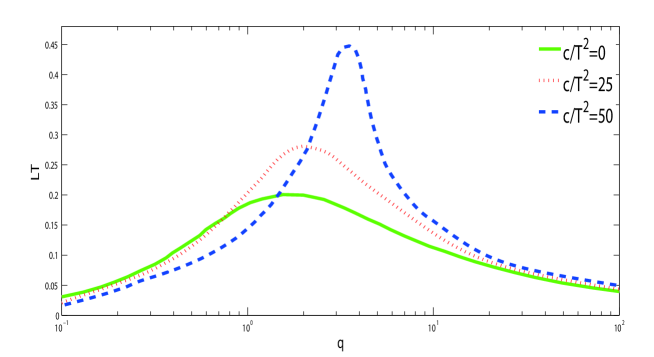
Figure 8: $LT$ as a function of $q$ at $\eta=1$ and $\theta=\frac{\pi}{3}$. different values of deformation parameter are contributed. The solid green curve corresponds to $\frac{c}{T^{2}}=0$, the dotted red curve to $\frac{c}{T^{2}}=25$ and the dashed blue curve to $\frac{c}{T^{2}}=50$.

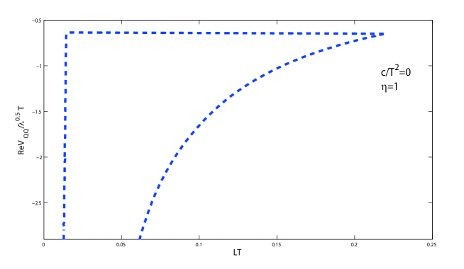
Figure 9: $ReV_{Q\bar{Q}}$ as a function of $LT$ at $\eta=1$ and $\theta=\frac{\pi}{3}$ and deformation parameter is zero

Figure 10: $ReV_{Q\bar{Q}}$ as a function of $LT$ at $\eta=1$ and $\theta=\frac{\pi}{3}$ and scaled deformation parameter is $\frac{c}{T^{2}}=25$

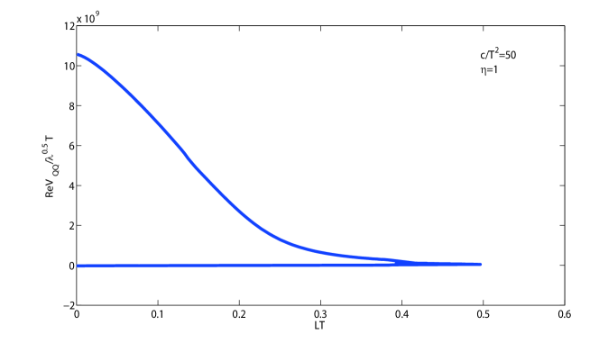
Figure 11: $ReV_{Q\bar{Q}}$ as a function of $LT$ at $\eta=1$ and $\theta=\frac{\pi}{3}$ and scaled deformation parameter is $\frac{c}{T^{2}}=50$

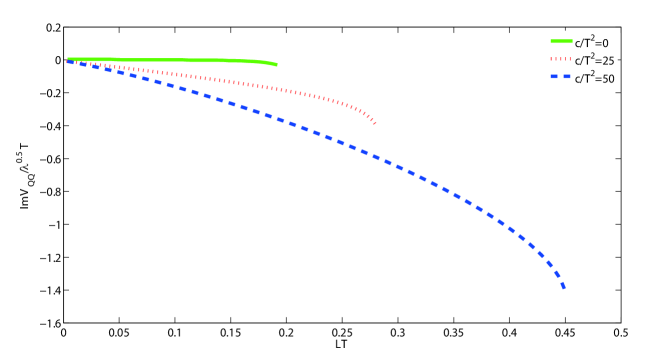
Figure 12: Imaginary part of potential as a function of $LT$, at a fixed velocity $\eta=1$ and $\theta=\frac{\pi}{3}$. different values of scaled deformation parameter are contributed. The solid green curve corresponds to $\frac{c}{T^{2}}=0$ , the dotted red curve to $\frac{c}{T^{2}}=25$ and the dashed blue curve to $\frac{c}{T^{2}}=50$.

We proceed by solving (3.29) numerically to have $y_{\ast}$ as a function of q and p, then (3.27), (3.28), (3.30), (3.31) will be functions of p and q. On the other hand for finding p as a function of q, one can solve (3.27) and (3.28) for fixed $\theta$, after doing all these, $LT$ as a function of q is in hand. Before we start to calculate $ImV_{Q\bar{Q}}$ we should obtain $\tilde{\theta}$, $y^{\prime\prime}(0)$ and $\tilde{b}$. The $\tilde{\theta}$ is obtained from (3.25) at $\tilde{\sigma}=0$ and $y=y_{\ast}$. We should solve (3.24) and (3.25) with use of boundary conditions (3.26) , to evaluate $y^{\prime\prime}(0)$ and $\tilde{b}$. After doing all these calculations numerically, with $y^{\prime\prime}(0)$ and $\tilde{b}$ known, we can calculate $ImV_{Q\bar{Q}}$ as a function of q. So, we will survey $LT(q)$ , also real and imaginary parts of potential as a function of $LT$.
The result of cases with a fixed $\eta$ and different choices of $\theta$ besides a fixed $\theta$ and different choices of $\eta$ have been studeid in sif , so we proceed by fixing both of them and choosing different values of deformation parameter.
In Fig. 8 we show $LT$ as a function of q for a fixed orientation of the dipole , fixed $\eta$ and different values of deformation parameter. we know $LT_{max}$ depends strongly on the rapidity $\eta$ and it decreases with increasing $\eta$ sif . In our plots, we can see that $LT_{max}$ which indicates the limit of validity of classical gravity calculation, increases with increasing deformation parameter.
In Figs. 9,10 and 11 we present $ReV_{Q\bar{Q}}$ as a function of LT. We can see for small values of LT which means short distances or small temperatures, there is a difference between $c=0$ and $c\neq 0$ cases. As we expected, when deformation parameter contributes to the calculation, the interaction of the pair is relevant with plasma, it is similar to the result of perpendicular case. The other point is that real part of potential has no intense alteration with varying angle for any value of deformation parameter.
In Fig. 12 we can see $ImV_{Q\bar{Q}}$ as a function of LT. It shows that for angle $\theta<\frac{\pi}{2}$ with decreasing angle, the imaginary part of potential becomes smaller for any values of deformation parameter.

4 Concolusion

In this article, we have used the method of sif to investigate the real and imaginary parts of potential for moving heavy quarkonia in plasma with a gravity dual which has deformation parameter in warp factor. At the first step we considered $Q\bar{Q}$ pair oriented perpendicularly to the hot wind and after that we extended all calculations to arbitrary angles. We saw that for both perpendicular and arbitrary angle cases, the limit of classical gravity calculation increases with increasing deformation parameter. Also for nonzero values of c the pair feels moving plasma even in short distances, but for $c=0$ case the pair does not feel moving plasma at some small values of LT as we expected. We indicated when nonzero values of deformation parameter contribute to the imaginary part of potential, the thermal width of quarkonia increases with increasing deformation parameter. Results of perpendicular case in compare with arbitrary angle $\theta<\frac{\pi}{2}$ showed that with decreasing angle, the imaginary part of potential becomes smaller for any values of deformation parameter, but real part of potential has no intense alteration with varying angle for any value of deformation parameter.
Another interesting problem is instead of using the soft wall model we use hyperscaling violation metric background and discuss the moving mesons and investigate real and imaginary parts of potential. This problem with corresponding metric background for the moving meson in plasma media is in hand.

Acknowledgement
The authors are grateful very much to S. M. Rezaei for support and valuable activity in numerical calculations.

References

- (1) N. Brambilla, M. A. Escobedo, J. Soto and A. Vairo, Heavy Quarkonium in a weakly-coupled quark-gluon plasma below the melting temperature, JHEP, 09 (2010) 038 [arxiv:1007.4156 [hep-ph]].
- (2) Y. Guo and M. Strickland, The imaginary part of the static gluon propagator in an anisotropic (viscous) QCD plasma,Phys. Rev. D, 79 (2009) 114003 [arxiv:0903.4703[hep-ph]]
- (3) M. Laine, O. Philipsen, P. Romatschke and M. Tassler, Real-time static potential in hot QCD, JHEP, 0703 (2007) 054 [arxiv:0611300 [hep-ph]]
- (4) A. Rothkopf, T. Hatsuda and S. Sasaki, Complex Heavy-Quark Potential at Finite Temperature from Lattice QCD, Phys. Rev. Lett. 108 (2012) 162001 [arxiv:1108.1579 [hep-lat]].
- (5) G. Aarts, C. Allton, S. Kim, M. P. Lombardo, M. B. Oktay, S. M. Ryan, D. K. Sinclair and J. I. Skullerud, What happens to the Upsilon and in the quark-gluon plasma? Bottomonium spectral functions from lattice QCD, JHEP, 1111 (2011) 103 [arxiv:1109.4496[hep-lat]].
- (6) G. Aarts, C. Allton, S. Kim, M. P. Lombardo, S. M. Ryan and J. I. Skullerud, Melting of P wave bottomonium states in the quark-gluon plasma from lattice NRQCD, JHEP, 1312 (2013) 064 [arxiv:1310.5467 [hep-lat]].
- (7) J. M. Maldacena, The Large N Limit of Superconformal Field Theories and Supergravity, Adv.Theor.Math.Phys, 2 (1998) 231 [arXiv: 9711200 [hep-th]] .
- (8) S. S. Gubster, I. R. Klebanov and A. M. Polyakov,Gauge Theory Correlators from Non-Critical String Theory, Phys. Lett. B, 428 (1998) 105 [arXiv: 9802109 [hep-th]].
- (9) E. Witten, Anti De Sitter Space And Holography, Adv. Theor. Math. Phys, 2 (1998) 253 [arXiv: 9802150 [hep-th]]
- (10) O. Aharony, S. S. Gubster, J. M. Maldacena, H. Ooguri and Y. Oz,Large N Field Theories, String Theory and GravityPhys. Rept, 323 (2000) 183 [arXiv: 9905111 [hep-th]]
- (11) J. Erlich, E. Katz, D. T. Son, M A Stephanov,QCD and a Holographic Model of Hadrons, Phys.Rev.Lett, 95 (2005) 261602 [arXiv: 0501128[hep-ph]].
- (12) H. R. Grigoryan and A. V. Radyushkin,Form Factors and Wave Functions of Vector Mesons in Holographic QCD, Phys. Lett. B, 650 (2007) 421 [arXiv: 0703069[hep-ph]].
- (13) H. R. Grigoryan and A. V. Radyushkin, Pion Form Factor in Chiral Limit of Hard-Wall AdS/QCD Model, Phys. Rev. D 76 (2007) 115007 [arXiv: 0709.0500 [hep-ph]].
- (14) E. Katz, A. Lewandowski and M. D. Schwartz,Tensors Mesons in AdS/QCD, Phys. Rev. D 74 (2006) 086004 [arXiv: 0510388[hep-ph]].
- (15) J. Polchinski and M. J Strassler,Hard Scattering and Gauge/String Duality, Phys. Rev. Lett 88 (2002) 031601 [arXiv: 0109174[hep-th]].
- (16) L. Da Rold and A. Pomarol, Chiral symmetry breaking from five dimensional spaces, Nucl. Phys. B 721 (2005) 79 [arXiv: 0501218[hep-ph]].
- (17) A. Karch, E. Katz, D. T. Son and M. A. Stephanov,Linear Confinement and AdS/QCD, Phys. Rev. D, 74 (2006) 015005 [arXiv: 0602229[hep-ph]].
- (18) S. J. Brodsky, G. F. de Teramond and A. Deur,Nonperturbative QCD Coupling and its β function from Light-Front Holography, Phys. Rev. D 81 (2010) 096010 [arXiv: 1002.3948[hep-ph]].
- (19) G. F. de Teramond and S. J. Brodsky, Gauge/Gravity Duality and Hadron Physics at the Light-Front, AIP Conf. Proc 1296 (2010) 128 [arXiv:1006.2431[hep-ph]].
- (20) W.D. Paula and T.Frederico,Scalar mesons within a dynamical holographic QCD model, Phys. Lett. B 693 (2010) 287291 [arXiv:0908.4282[hep-ph]]
- (21) H. Forkel, M. Beyer and T. Frederico, Linear square-mass trajectories of radially and orbitally excited hadrons in holographic QCD, JHEP 0707 (2007) 077 [arXiv: 0705.1857 [hep-ph]].
- (22) W. de Paula, T. Frederico, H. Forkel and M. Beyer,Dynamical holographic QCD with area-law confinement and linear Regge trajectories, Phys. Rev. D 79 (2009) 075019 [arXiv:0806.3830[hep-ph]].
- (23) B. Galow, E. Megias, J. Nian and H. J. Pirner, Phenomenology of AdS/QCD and Its Gravity Dual, Nucl. Phys. B 834 (2010) 330 [arXiv: 0911.0627[hep-ph]].
- (24) J. Nian and H. J Pirner, Wilson Loop-Loop Correlators in AdS/QCD, Nucl. Phys. A 833 (2010) 119 [arXiv: 0908.1330[hep-ph]].
- (25) H. R. Grigoryan and A. V. Radyushkin, Structure of Vector Mesons in Holographic Model with Linear Confinement, Phys. Rev. D 76 (2007) 095007 [arXiv: 0706.1543[hep-ph]].
- (26) H. Forkrl, Holographic glueball structure, Phys. Rev. D 78 (2008) 025001 [arXiv:0711.1179 [hep-ph]].
- (27) H. J. Kwee and R. F. Lebed,Pion Form Factor in Improved Holographic QCD Backgrounds, Phys. Rev. D 77 (2008) 115007 [arXiv: 0712.1811[hep-ph]].
- (28) P. Colangleo, F. De Fazio, F. Jugeau and S. Nicotri, On the light glueball spectrum in a holographic description of QCD, Phys. Lett. B 652 (2007) 73 [arXiv: 0703316[hep-ph]].
- (29) A. Vega and I. Schmidt, Hadrons in AdS / QCD correspondence, Phys. Rev. D 79 (2009) 055003 [arXiv: 0811.4638[hep-ph]].
- (30) A. Vega, I Schmidt, T Branz, T Gutsche and V E Lyubovitskij, Meson wave function from holographic models, Phys. Rev. D 80 (2009) 055014 [arXiv: 0906.1220[hep-ph]].
- (31) A. Vega and . Schmidt,Modes with variable mass as an alternative in AdS / QCD models with chiral symmetry breaking, Phys. Rev. D 82 (2010) 115023 [arXiv:1005.3000 [hep-ph]].
- (32) G. F. de Teramond and S. J. Brodsky, Light-Front Quantization Approach to the Gauge-Gravity Correspondence and Hadron Spectroscopy, AIP Conf. Proc 1257 (2007) 59 [arXiv: 1001.5193[hep-ph]].
- (33) Z. Abidin and C. E. Carlson,Nucleon electromagnetic and gravitational form factors from holography, Phys. Rev. D, 79 (2009) 115003 [arXiv: 0903.4818[hep-ph]].
- (34) T. Branz, T. Gutsche, V. E. Lyubovitskij, I. Schmidt and A. Vega, Light and heavy mesons in a soft-wall holographic approach, Phys. Rev. D 82 (2010) 074022 [arXiv:1008.0268[hep-ph]].
- (35) A. Vega, I. Schmidt, T. Gutsche and V. E. Lyubovitskij, Generalized parton distributions in AdS/QCD, Phys. Rev. D 83 (2011) 036001 [arXiv: 1010.2815[hep-ph]].
- (36) M. Strickland,Thermal Upsilon(1s) and suppression in Pb-Pb collisions at the LHC, Phys. Rev. Lett 107 (2011) 132301 [arXiv:1106.2571[hep-ph]].
- (37) M. Strickland and D. Bazow,Thermal Bottomonium Suppression at RHIC and LHC, Nucl. Phys. A 879 (2012) 25 [arXiv:1112.2761[nucl-th]].
- (38) M. Margotta, K. McCarty, C. McGahan, M. Strickland, and D. Yager-Elorriaga, Quarkonium states in a complex-valued potential, Phys.Rev.D 83 (2011) 105019 [arXiv:1101.4651 [hep-ph]].
- (39) G.Aarts, C. Allton, S. Kim, M. P. Lombardo, M. B. Oktay, S. M. Ryan, D. K. Sinclair and J. I. Skullerud,S wave bottomonium states moving in a quark-gluon plasma from lattice NRQCD, JHEP 1303 (2013) 084 [arXiv:1210.2903[hep-lat]].
- (40) S. I. Finazzo and J. Noronha,Thermal suppression of moving heavy quark pairs in strongly coupled plasma [arXiv: 1406.2683[hep-th]].
- (41) S. I. Finazzo and J. Noronha,Estimates for the Thermal Width of Heavy Quarkonia in Strongly Coupled Plasmas from Holography, JHEP 1311 (2013) 042 [arXiv:1306.2613[hep-ph]].
- (42) J. Erlich, E. Katz, D. T. Son and M. A. Stephanov, QCD and a Holographic Model of Hadrons, Phys. Rev. Lett 95 (2005) 261602 [arxiv:0501128 [hep-ph]]
- (43) G. F. de Teramond and S. J. Brodsky, Hadronic Spectrum of a Holographic Dual of QCD, Phys. Rev. Lett 94 (2005) 201601 [arxiv:0501022 [hep-th]]
- (44) J. Babington, J. Erdmenger, N. J. Evans, Z. Guralnik and I. Kirsch, Chiral Symmetry Breaking and Pions in Non-Supersymmetric Gauge/Gravity Duals, Phys. Rev. D 69 (2004) 066007 [arXiv:0306018[hep-th]].
- (45) M. Kruczenski, D. Mateos, R. C. Myers and D. J. Winters, Towards a holographic dual of large- QCD, JHEP 0405 (2004) 041 [arxiv:0311270 [hep-th]]
- (46) T. Sakai and S. Sugimoto, Low energy hadron physics in holographic QCD, Prog.Theor. Phys 113 (2005) 843 [arXiv:0412141[hep-th]].
- (47) T. Sakai and S. Sugimoto, More on a holographic dual of QCD, Prog. Theor. Phys 114 (2006) 1083 [arXiv:0507073[hep-th]].
- (48) S. He, M. Huang, Q. S. Yan and Y. Yang, Confront Holographic QCD with Regge Trajectories of vectors and axial-vectors, Eur.Phys.J.C 66 (2010) 187, [arXiv:0710.0988 [hep-ph]].
- (49) A. Karch, E. Katz, D. T. Son and M. A. Stephanov, Linear Confinement and AdS/QCD, Phys. Rev. D 74, (2006) 015005 [arXiv:0602229[hep-ph]]
- (50) O. Andreev and V. I. Zakharov, Heavy-Quark Potentials and AdS/QCD, Phys.Rev. D 74 (2006) 025023 [arXiv:0604204[hep-ph]].
- (51) F. Zuo, Improved soft-wall model with a negative dilaton, Phys. Rev. D 82 (2010) 086011 [arXiv:0909.4240 [hep-ph]].
- (52) G. F. de Teramond and S. J. Brodsky, Light-Front Holography and Gauge/Gravity Duality: The Light Meson and Baryon Spectra, Nucl.Phys.Proc.Suppl, 199 (2010) 89 [arXiv:0909.3900 [hep-ph]].
- (53) J. P. Shock, F. Wu, Y. L. Wu and Z. F. Xie, AdS/QCD Phenomenological Models from a Back-Reacted Geometry, JHEP 0703 (2007) 064 [arxiv:0611227 [hep-ph]]
- (54) K. Ghoroku, M. Tachibana and N. Uekusa,Dilaton coupled brane-world and field trapping, Phys. Rev. D 68 (2003) 125002 [arXiv:0304051[hep-th]].
- (55) K. Ghoroku, N. Maru, M. Tachibana and M. Yahiro, Holographic Model for Hadrons in Deformed AdS5 Background, Phys. Lett. B 633, (2006 ) 602 [arXiv:0510334[hep-ph]].
- (56) C. Csaki and M. Reece, Toward a Systematic Holographic QCD: A Braneless Approach, JHEP 0705 (2007) 062 [arXiv:0608266[hep-ph]].
- (57) U. Gursoy and E. Kiritsis, Exploring improved holographic theories for QCD: Part I, JHEP 0802 (2008) 032 [arXiv:0707.1324 [hep-th]].
- (58) U. Gursoy, E. Kiritsis and F. Nitti, Exploring improved holographic theories for QCD: Part II, JHEP 0802 (2008) 019 [arXiv:0707.1349 [hep-th]].
- (59) D. f. Zeng, Heavy Quark Potentials in Some Renormalization Group Revised AdS/QCD Models, Phys. Rev. D 78 (2008) 126006 [arXiv:0805.2733 [hep-th]].
- (60) H. J. Pirner and B. Galow, Equivalence of the AdS-Metric and the QCD Running Coupling, Phys. Lett. B 679 (2009) 51 [arXiv:0903.2701 [hep-ph]].
- (61) S. He, M. Huang and Q. S. Yan, Logarithmic correction in the deformed AdS5 model to produce the heavy quark potential and QCD beta function, Phys. Rev. D, 83 (2011) 045034 [arXiv:1004.1880 [hep-ph]].
- (62) D. Li, S. He, M. Huang and Q. S. Yan, Thermodynamics of deformed model with a positive/negative quadratic correction in graviton-dilaton system, JHEP 1109 (2011) 041 [arXive:1103.5389 [hep-th]].
- (63) U. Gürsoy, E. Kiritsis, G. Michalogiorgakis and F. Nitti,Thermal Transport and Drag Force in Improved Holographic QCD, JHEP 0912 (2009) 056 [arxiv:0906.1890 [hep-ph]].
- (64) J. Casalderrey, H. Liu, D. Mateos, K. Rajagopal and U. A. Wiedemann, Gauge/String Duality, Hot QCD and Heavy Ion Collisions, CERN-PH-TH (2010) 316 [arxiv:1101.0618 [hep-th]].