Fluctuation of strongly interacting matter in Polyakov Nambu Jona-Lasinio model in finite volume

Abstract

We estimate the susceptibilities of conserved charges for two flavor strongly interacting matter with varying system sizes, using the Polyakov loop enhanced Nambu–Jona-Lasinio model. The susceptibilities for vanishing baryon densities are found to show a scaling with the system volume in the hadronic as well as partonic phase. This scaling breaks down for a temperature range of about 30-50 MeV around the crossover region. Simultaneous measurements of the various susceptibilities may, thus, indicate how close to the crossover region the freeze-out occurs for the fireball created in heavy-ion collision experiments.

Strongly interacting matter under extreme conditions of temperature and density is expected to show a rich phase structure. In the early Universe, a few microsecond after the Big Bang, when the temperature was extremely high, exotic states namely quarks and gluons may have been prevalent kolb . On the other hand inside the core of a compact star, where the baryon matter density is extremely high various exotic phases like color superconductor, color superfluid etc. may be present rajagopal . Experiments with heavy ions colliding with each other or with a target, at the facilities at CERN(France/Switzerland), BNL(USA) and GSI(Germany), are continuing the search for such exotic states of matter in the laboratory.

The matter formed due to the energy deposition of the colliding particles obviously has a finite volume. It is therefore imperative to have a clear understanding of the finite size effects to fully contemplate the thermodynamic phases that may be created in the experiments. These effects depend on the size of the colliding nuclei, the center of mass energy ($\sqrt{s}$) and the centrality of collisions. There have been a large number of efforts to estimate the system size at freeze-out for different $\sqrt{s}$ and different centralities. A study using the measurement of HBT radii ceres indicates that the freeze out volume increases as the $\sqrt{s}$ increases. In the same work the freeze out volume has been estimated to be $2000~{}fm^{3}$ to $3000~{}fm^{3}$. On the other hand in Ref. graf the volume of homogeneity has been calculated using UrQMD model urqmd and compared with the experimentally available results. The $\sqrt{s}$ considered was in the range of 62.4 GeV to 2760 GeV for lead-lead collisions at different centralities. The system volume has been found to vary from $50~{}fm^{3}$ to $250~{}fm^{3}$. The effect of colliding particles and $\sqrt{s}$ has been further analyzed by the ALICE collaboration in alice-fs . Given that these are the volumes at the time of freeze-out, one may expect an even smaller system size at the initial equilibration time initi-fs1 ; initi-fs2 .

The importance of finite size effects in the thermodynamics of strong interaction may be brought forward with the help of finite size scaling analysis fss . In the context of heavy ion collisions such a possible analysis has been discussed in the literature (see e.g. fss1 ; fss2 ; fss3 ).

Other theoretical studies of finite volume effects have been performed in various contexts. In Ref. elze the effective degrees of freedom have been found to be reduced due to finite volume using a non-interacting bag model. The effect of finite volume has been studied also with a two model equation of state and it has been found that the critical temperature looses its sharpness spieles . A few first principle study of pure gluon theory on space-time lattices were performed, showing the possibility of significant finite size effects fslat1 ; fslat2 . The meson properties show a significant volume dependence as found in Ref. fischer1 ; fischer2 . In the context of chiral perturbation theory the implications of finite system size have been discussed lusher1 ; gasser1 . There are also studies with four-fermi type interactions, like the Nambu$-$Jona-Lasinio (NJL) Nambu models kiriyama ; fss1 ; shao , linear sigma models fss2 ; braun1 ; braun2 and Gross-Neveu models khanna . While in Ref. braun1 the scaling behavior of chiral phase transition for finite and infinite volumes has been studied, the character of phase diagram has been studied in Ref. fss1 ; fss2 ; braun2 ; khanna . In refs. kiriyama and shao the authors have studied the chiral properties as a function of the radius of a finite droplet of quark matter. The stability of such a droplet in the context of strangelet formation within the NJL model has been addressed in Ref. yasui . Size dependent effects of di-fermion states within 2-dimensional NJL model has been studied in Ref. abreu1 and that of magnetic field is discussed in Ref. abreu2 . Recently in a 1+1 dimensional NJL model the induction of charged pion condensation phenomenon in dense baryonic matter due to finite volume effects have been studied in ebert . Recently some of us have studied the thermodynamic properties of strongly interacting matter in a finite volume using Polyakov-Nambu-Jona–Lasinio (PNJL) model ab . It has been shown there that the critical temperature for the cross-over transition at zero baryon density decreases as the volume decreases. Furthermore at low volume the critical end point is pushed towards the higher $\mu$ and lower $T$ domain. At $R=2fm$, it was found that the critical end point (CEP) vanishes and the whole phase diagram becomes a cross-over. The possible chiral symmetry restoration in a color confined state has also been discussed.

Though various thermodynamic properties have been studied to some extent in finite size systems, not much has been done to estimate the fluctuations occurring in finite volumes. On the lattice, the Polyakov loop susceptibility has been calculated for a finite volume berg . A similar work has been done in the PNJL model using Monte Carlo simulation cristoforetti and also in the quark-meson model using a renormalisation group approach tripolt . Fluctuations of conserved quantum numbers are related to the respective susceptibilities via the fluctuation-dissipation theorem. For a 2-flavor strongly interacting system one has the quark number susceptibility (QNS) and isospin number susceptibility (INS) etc. These fluctuations are sensitive indicators of the transition from hadronic matter to partonic state. Also the existence of the CEP may be signalled by the diverging behavior of fluctuations. Here we report our calculations of quark and isospin number susceptibilities of strongly interacting matter using PNJL model up to sixth order. The report is organized as follows. First we give a very brief description of the PNJL model and the necessary methodology. Thereafter we present the results for the various susceptibilities. Finally we summarize and conclude.

The PNJL model used here is based on a series of works  Nambu ; ab ; klev ; hat1 ; fuku ; ratti ; MAS3_2006 ; ray1 ; ray2 ; MAS_12 ; MAS_14 ; aminul1 ; MAS1_2006 ; MAS2_2006 ; Muller . For some recent progress in this model see e.g. shear ; vphimu ; isospin ; aminul1 ; quarkyonic ; shear1 ; charge ; avg_phase_pnjl ; CP_pnjl ; color_pnjl1 ; color_pnjl2 . For a detailed overview see e.g. ray3 and references therein. The PNJL model for 2 flavors is described by the Lagrangian,

$${\cal L} ={\sum_{f=u,d}}{\bar{\psi}_{f}}\gamma_{\mu}iD^{\mu}{\psi_{f}}-\sum_{f}m_{f}{\bar{\psi}_{f}}{\psi_{f}}+\sum_{f}\mu_{f}\gamma_{0}{\bar{\psi}_{f}}{\psi_{f}}$$

$$+{\frac{g_{S}}{2}}{\sum_{a=1,2,3}}[({\bar{\psi}}\tau^{a}{\psi})^{2}+({\bar{\psi}}i\gamma_{5}\tau^{a}{\psi})^{2}]-{\cal{U^{\prime}}}(\Phi[A],\bar{\Phi}[A],T)$$ (1)

where Polyakov loop potential ${{\cal{U^{\prime}}}(\Phi[A],\bar{\Phi}[A],T)}$ can be expressed as,

$$\frac{{\cal{U^{\prime}}}(\Phi[A],\bar{\Phi}[A],T)}{T^{4}}=\frac{{\cal U}(\Phi[A],\bar{\Phi}[A],T)}{{T^{4}}}-\kappa\ln(J[\Phi,{\bar{\Phi}}])$$ (2)

Here ${\cal U}(\Phi,{\bar{\Phi}},T)$ is a Landau-Ginsburg type potential as given in Ref. ratti ,

$$\frac{{\cal U}(\Phi,\bar{\Phi},T)}{{T^{4}}}=-\frac{{b_{2}}(T)}{2}{\bar{\Phi}}\Phi-\frac{b_{3}}{6}(\Phi^{3}+\bar{\Phi}^{3})+\frac{b_{4}}{4}{(\bar{\Phi}\Phi)}^{2},$$ (3)

where

$${b_{2}}(T)=a_{0}+{a_{1}}(\frac{{T_{0}}}{T})+{a_{2}}(\frac{{T_{0}}}{T})^{2}+{a_{3}}(\frac{{T_{0}}}{T})^{3},$$ (4)

$b_{3}$ and $b_{4}$ being constants. The second term in Eqn.(2) is the Vandermonde term.

$$J[\Phi,{\bar{\Phi}}]=(27/24{\pi^{2}})\left[1-6\Phi{\bar{\Phi}}+\\ 4(\Phi^{3}+{\bar{\Phi}}^{3})-3{(\Phi{\bar{\Phi}})}^{2}\right]$$

The parameters $a_{i}$, $b_{i}$ were fitted from Lattice results of pure gauge theory. The set of values chosen here are,

$a_{0}=6.75$, $a_{1}=-1.95$, $a_{2}=2.625$, $a_{3}=-7.44$, $b_{3}=0.75$, $b_{4}=7.5$, $T_{0}=190MeV$, $\kappa=0.2$

To incorporate the effect of finite volume we use a non-zero low momentum cut-off $p_{min}=\pi/R=\lambda$ where $R$ is the lateral size of a cubic volume $V=R^{3}$. In principle one should sum over discrete momentum values but for simplification we integrate over continuous values of momentum. Also we neglect surface and curvature effects. Other parameters of the model were not modified.

We note here that in the NJL model discussions of using a lower momentum cut-off exists in the literature (see ebert1 ; blaschke and references therein). The motivation of introducing this IR cut-off there has been to mimic confining effects of strong interaction which helps to remove spurious poles in the quark loop diagrams so that unphysical decay of hadrons to quarks do not take place. Since in the PNJL model such unphysical decays are restricted due to the vanishing of the Polyakov loop for low temperatures ratti ; blaschke1 no IR cut-off is necessary in the PNJL model. However, for 2 flavour PNJL model, the unphysical decay does not completely vanish as pointed out in Ref. prd75 where a very small but non-zero sigma meson decay is observed at low temperatures. On the other hand, for 2+1 flavour the $\sigma$-meson becomes a true bound state for small temperatures prd79 .

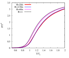
Figure 1: (Color online) Variation of pressure with temperature for different system sizes.

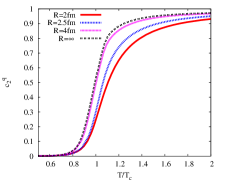
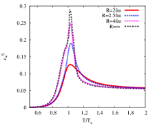
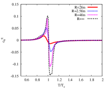
Figure 2: (Color online) Variation of quark number susceptibilities with temperature for different system sizes.

Our starting point is the thermodynamic potential given by,

$$\Omega ={\cal{U^{\prime}}}[\Phi,\bar{\Phi},T]+2{g_{S}}{\sum_{f=u,d}}{\sigma_{f}^{2}}-6{\sum_{f}}{\int_{\lambda}^{\Lambda}}\frac{{d^{3}p}}{{(2\pi)}^{3}}E_{p_{f}}\Theta{(\Lambda-{|\vec{p}|})}$$

$$-2{\sum_{f}}T{\int_{\lambda}^{\infty}}\frac{{d^{3}p}}{{(2\pi)}^{3}}\ln\left[1+3(\Phi+{\bar{\Phi}}\exp(\frac{-(E_{p_{f}}-\mu_{f})}{T}))\exp(\frac{-(E_{p_{f}}-\mu_{f})}{T})+\exp(\frac{-3(E_{p_{f}}-\mu_{f})}{T})\right]$$

$$-2{\sum_{f}}T{\int_{\lambda}^{\infty}}\frac{{d^{3}p}}{{(2\pi)}^{3}}\ln\left[1+3({\bar{\Phi}}+{\Phi}\exp(\frac{-(E_{p_{f}}+\mu_{f})}{T}))\exp(\frac{-(E_{p_{f}}+\mu_{f})}{T})+\exp(\frac{-3(E_{p_{f}}+\mu_{f})}{T})\right]$$ (5)

where $E_{p_{f}}=\sqrt{p^{2}+M^{2}_{f}}$ is the single quasi-particle energy. In the above expression $\sigma_{f}$ is given as

$$\sigma_{f}=\langle{\bar{\psi}}_{f}\psi_{f}\rangle=-\frac{3{M_{f}}}{{\pi}^{2}}{\int^{\Lambda}_{\lambda}}\frac{p^{2}}{\sqrt{p^{2}+{M_{f}}^{2}}}dp,$$ (6)

We first obtain the mean fields $\sigma$, $\Phi$ and $\bar{\Phi}$ from the extremization conditions: $\frac{\partial\Omega}{\partial\sigma}=0,~{}~{}~{}\frac{\partial\Omega}{\partial\Phi}=0,~{}~{}~{}\frac{\partial\Omega}{\partial\bar{\Phi}}=0$. The field values so obtained are then put back into $\Omega$ to obtain the thermodynamic potential, which is then used to obtain various thermodynamic quantities. Some of which have been reported by us in Ref. ab . For example, the pressure in the finite volume system is given by,

$$P(T,\mu_{q},\mu_{I})=-\frac{\partial(\Omega(T,\mu_{q},\mu_{I})V)}{\partial V}$$ (7)

where $T$ is the temperature and $\mu_{q}$ and $\mu_{I}$ are the quark and isospin chemical potentials respectively. The variation of scaled pressure with $T/T_{c}$ is shown in figure 1. The critical temperature $T_{c}$ is dependent on the system size. We have considered different system sizes corresponding to $R=2~{}fm$, $R=2.5~{}fm$, $R=4~{}fm$ and infinite volume. The corresponding values of $T_{c}$ are 167 MeV, 171 MeV, 183 MeV and 186 MeV respectively.

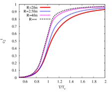
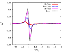
Figure 3: (Color online) Variation of isospin number susceptibilities with temperature for different system sizes.

We now discuss the various susceptibilities of quark number and iso-spin number. These are defined as,

$$c_{n}(T)=\frac{1}{n!}\frac{\partial^{n}\left({\Omega(T,\mu_{q},\mu_{I})/T^{4}}\right)}{\partial\left(\frac{\mu_{X}}{T}\right)^{n}}\Big{|}_{\mu_{X}=0}~{}~{}~{}.$$ (8)

where $\mu_{X}=\mu_{q}$ or $\mu_{I}$. For an expansion around $\mu_{X}=0$, the odd order terms vanish due to CP symmetry. Many of these susceptibilities have been measured for infinite volume systems in first principle QCD calculations on the lattice Gottieb_prl ; Gottieb_prd ; Alton ; Gavai_prd1 ; Gavai_prd2 ; HOTQCD_08 ; Cheng_09 ; WB_12 ; HOTQCD_12 as well as hard thermal loop calculations Blaizot ; purnendu1 ; purnendu2 ; jiang ; HTLPT_Najmul ; najmul ; HMS1_2013 ; HMS2_2013 ; HAMSS_2014 ; HBAMSS_2014 . At the same time various QCD inspired models have also made suitable estimates of these fluctuations for infinite systems (see e.g. ray1 ; ray2 ; ray3 ; sasaki_redlich ; FLW_2010 ; abhijit ; abhijit1 ; roessner1 ; friman ; roessner2 ; schaefer1 ; schaefer2 ; schaefer3 ; schaefer4 ) Here we present the first computation of finite size effects on these fluctuations.

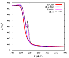
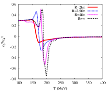
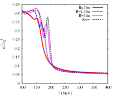
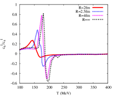
Figure 4: (Color online) Variation of ratios of fluctuations with temperature for different system sizes.

For each system volume considered, we have calculated $\Omega$ at chemical potentials spaced by 0.1 MeV at a given temperature. These have been fitted it to an eighth order polynomial in $\mu_{X}$ using the GNU plot program. We have chosen the maximum range of $\mu_{X}$ to be 200 MeV. From the fit we have extracted the coefficients $c_{2}$, $c_{4}$ and $c_{6}$ both for quark number and isospin number susceptibilities. This procedure has been repeated for different values of temperature.

The variation of quark number susceptibilities with $T/T_{c}$ are shown in Fig. (2). The general features for these susceptibilities in finite volumes are quite similar to that for infinite volume. However quantitatively we observe significant volume dependence. With increase in system size there is an enhancement of all the susceptibilities. For the isospin number susceptibilities shown in figure 3, we find almost identical behavior. It may be noted that the most significant finite size effects are seen in the higher order susceptibilities close to the cross-over region. Given that the detectors in QGP search experiments are expected to observe the system frozen close to the cross-over region, one may find an estimate of the system volume from the measurement of various higher order fluctuations.

Alternatively, it is important to realize that for a comparison of fluctuations calculated theoretically with that measured experimentally, one needs to be confident about the measured system volumes. Since measuring the system size is quite a difficult task in the experiments, and one usually resorts to consider ratios of fluctuations to eliminate the volume factor Alton . However this assumption is valid when interactions are small and the volume factor scales out. Therefore in the purely hadronic or partonic phases one may observe such a scaling of the fluctuations with system size. However, close to the cross-over region such an assumption may not hold as large scale fluctuations are dominant and the system deviates from a stable thermodynamic phase. Now that we have the actual calculations of system size effects we can easily check the how the ratio of fluctuations behave. For this purpose we present the ratios $c_{4}/c_{2}$ (kurtosis) and $c_{6}/c_{4}$ for both the quark number and isospin number susceptibilities. In this case we obviously need to plot the variation with temperature rather than with $T/T_{c}$. The variations are shown in Fig. (4). We observe that for low and high temperatures the ratios of fluctuations show the expected scaling with the system volume, while in the cross-over region there is significant volume dependence. Thus if the system created in heavy-ion experiments freeze-out much below $T_{c}$, the ratios of different susceptibilities would show the corresponding values for the hadronic phase. The amount of deviation of these ratios from the hadronic phase results would indicate the closeness of the system to the cross-over region.

To summarize, we have studied the fluctuations of strongly interacting matter in a finite volume using the PNJL model. The susceptibilities in the quark number and isospin number are obtained up to sixth order for different system sizes. We find a significant volume dependence in these quantities, which may be useful in analyzing the experimental data and obtain the size of the fireball formed in the heavy-ion collision experiments. The volume dependence shows an expected scaling behavior in the hadronic and partonic phases. In the cross-over region the system size scaling breaks down and may be use to estimate the closeness of the created fireball to the cross-over region. Given that all our present analysis is at zero density the results are suitable for analyzing LHC data.

The work is funded by Department of Science and Technology (DST) (Government of India) and Alexander von Humboldt (AvH) foundation.

References

- (1) E. W. Kolb and M. S. Turner, in The Early Universei, Front. Phys. 69, 1 (1990).
- (2) K. Rajagopal and F. Wilczek, in At the frontier of particle physics, edited by M. Shifman, (World Scientific, Singapore, 2001). (arXiv:hep-ph/0011333).
- (3) D. Adamova et. al., Phys. Rev. Lett. 90, 022301 (2003).
- (4) G. Graef, M. Bleicher and Q. Li, Phys. Rev. C 85, 044901 (2012).
- (5) S. Bass et. al., Prog. Part. Nucl. Phys. 41, 225 (1998); M. Bleicher et. al., J. Phys. G 25, 1859 (1999); H. Petersen, J. Steinheimer, G. Burau, M. Bleicher and H. Stöcker Phys. Rev. C 78, 044901 (2008).
- (6) B. Abelev et. al. (ALICE Collaboration), Phys. Lett. B 739, 139 (2014).
- (7) P. Bozek and W. Broniowski, Phys. Lett. B 720, 250 (2013).
- (8) A. Bzdak, B. Schenke, P. Tribedy and R. Venugopalan Phys. Rev. C 87, 064906 (2013).
- (9) A. E. Ferdinand and M. E. Fisher, Phys. Rev. 185, 832 (1969); M. E. Fisher and M. N. Barber, Phys. Rev. Lett. 28, 1516 (1972); M. N. Barber, in Phase Transitions and Critical Phenomenon, edited by C. Domb and J. L. Lebowitz, (Academic Press), 8, 146 (1987); J. L. Cardy, Scaling and Renormalization in Statistical Physics, (Cambridge, New York, 1996); D. Amit, Field Theory, The Renormalization Group and Critical Phenomena, (World Scientific, Singapore, 2005).
- (10) L. M. Abreu, M. Gomes and A. J. da Silva, Phys. Lett. B 642, 551 (2006).
- (11) L. F. Palhares, E. S. Fraga and T. Kodama, J. Phys. G 38, 085101 (2011).
- (12) E. S. Fraga, L. F. Palhares and P. Sorensen, Phys. Rev. C 84, 011903(R) (2011).
- (13) H.-T. Elze and W. Greiner, Phys. Lett. B 179, 385 (1986).
- (14) C. Spieles, H. Stoecker and C. Greiner, Phys. Rev. C 57, 908 (1998).
- (15) A. Gopie and M. C. Ogilvie, Phys. Rev. D 59, 034009 (1999).
- (16) A. Bazavov and B. A. Berg, Phys. Rev. D 76, 014502 (2007).
- (17) C. S. Fischer and M. R. Pennington, Phys. Rev. D 73, 034029 (2006).
- (18) J. Luecker, C. S. Fischer and R Williams, Phys. Rev. D 81, 094005 (2010).
- (19) M. Luscher, Commun. Math. Phys. 104, 177 (1986).
- (20) J. Gasser and H. Leutwyler, Phys. Lett. B 188, 477 (1987).
- (21) Y. Nambu and G. Jona-Lasinio, Phys. Rev. 122, 345 (1961); 124, 246 (1961).
- (22) O. Kiriyama and A. Hosaka, Phys. Rev. D 67, 085010 (2003).
- (23) G. Shao, L. Chang, Y. Liu and X. Wang, Phys. Rev. D 73, 076003 (2006).
- (24) J. Braun, B. Klein and P. Piasecki, Eur. Phys. Jr. C 71, 1576 (2011).
- (25) J. Braun, B. Klein and B.-J. Schefer, Phys. Lett. B 713, 216 (2012).
- (26) F. C. Khanna, A. P. C. Malbouisson, J. M. C. Malbouisson and A. E. Santana, Eur. Phys. Lett. 97, 11002 (2012).
- (27) S. Yasui and A. Hosaka, Phys. Rev. D 74, 054036 (2006).
- (28) L. M. Abreu, A. P. C. Malbouisson and J. M. C. Malbouisson, Phys. Rev. D 83, 025001 (2011).
- (29) L. M. Abreu, A. P. C. Malbouisson and J. M. C. Malbouisson, Phys. Rev. D 84, 065036 (2011).
- (30) D. Ebert, T. G. Khunjua, K. G. Klimenko and V. Ch. Zhukovsky, Int. Jr. Mod. Phys. A 27, 1250162 (2012).
- (31) A. Bhattacharyya, P. Deb, S. K. Ghosh, R. Ray and S. Sur, Phys. Rev. D 87, 054009 (2013).
- (32) B. A. Berg and H. Wu, Phys. Rev. D 88, 074507 (2013).
- (33) M. Cristoforetti, T. Hell, B. Klein and W. Weise, Phys. Rev. D 81, 114017 (2010).
- (34) R. Tripolt, J. Braun, B. Klein and B. Schaefer, Phys. Rev. D 90, 054012 (2014).
- (35) S. P. Klevansky, Rev. Mod. Phys. 64, 649 (1992).
- (36) T. Hatsuda and T. Kunihiro, Phys. Rept. 247, 221 (1994).
- (37) K. Fukushima, Phys. Lett. B 591, 277 (2004).
- (38) C. Ratti, M. A. Thaler and W. Weise, Phys. Rev. D 73, 014019 (2006).
- (39) E. Megías, E. R. Arriola and L. L. Salcedo, Jr. High Energy Phys. 0601, 73 (2006).
- (40) S. K. Ghosh, T. K. Mukherjee, M. G. Mustafa and R. Ray, Phys. Rev. D 73, 114007 (2006); S. Mukherjee, M. G. Mustafa and R. Ray, Phys. Rev. D 75, 094015 (2007).
- (41) S. K. Ghosh, T. K. Mukherjee, M. G. Mustafa and R. Ray, Phys. Rev. D 77, 0904024 (2008).
- (42) E. Megías, E. R. Arriola and L. L. Salcedo, Phys. Rev. Lett. 109, 151601 (2012).
- (43) E. Megías, E. R. Arriola and L. L. Salcedo, Phys. Rev. D 89, 076006 (2014).
- (44) C. A. Islam, R. Abir, M. G. Mustafa, R. Ray and S. K. Ghosh, J. Phys. G 41, 025001 (2014).
- (45) E. Megías, E. R. Arriola and L. L. Salcedo, Phys. Rev. D 74, 065005 (2006).
- (46) E. Megías, E. R. Arriola and L. L. Salcedo, Phys. Rev. D 74, 114014 (2006).
- (47) H.-M. Tsai and B. Müller; J. Phys. G 36, 075101 (2009).
- (48) S. K. Ghosh, S. Raha, R. Ray, K. Saha and S. Upadhaya, arXiv:1411.2765 [hep-ph].
- (49) X. Xin, S. Qin and Y. Liu, Phys. Rev. D 89, 094012 (2014).
- (50) A. Bhattacharyya, S. K. Ghosh, A. Lahiri, S. Majumder, S. Raha and R. Ray, Phys. Rev. C 89, 064905 (2014).
- (51) M. Dutra, O. Lourenc, A. Delfino, T. Frederico and M. Malheiro, Phys. Rev. D 88, 114013 (2013).
- (52) R. Marty, E. Bratkovskaya, W. Cassing, J. Aichelin and H. Berrehrah, Phys. Rev. C 88, 045204 (2013).
- (53) A. Bhattacharyya, S. Das, S. K. Ghosh, S. Raha, R. Ray, K. Saha and S. Upadhaya, arXiv:1212.6010 [hep-ph].
- (54) Y. Sakai, T. Sasaki, H. Kouno and M. Yahiro, Phys. Rev. D 82, 096007 (2010).
- (55) J. K. Boomsma and D. Boer, Phys. Rev. D 80, 034019 (2009).
- (56) H. Abuki, M. Ciminale, R. Gatto and M. Ruggieri, Phys. Rev. D 79, 034021 (2009).
- (57) H. Abuki and K. Fukushima, Phys. Lett. B 676, 57 (2009).
- (58) S. K. Ghosh, A Lahiri, S. Majumder, M. G. Mustafa, S. Raha and R. Ray, Phys. Rev. D 90, 054030 (2014).
- (59) D. Ebert, T. Feldmann and H. Reinhardt, Phys. Lett. B 388, 154 (1996).
- (60) D. Blaschke, G. Burau, M. K. Volkov and V. L. Yudichev, Eur. Phys. J. A 11, 319 (2001); A. Dubinin, D. Blaschke and Y. L. Kalinovsky, Acta Phys. Polon. Supp. 7, 215 (2014).
- (61) D. Blaschke, A. Dubinin and M. Buballa, arXiv:1412.1040 [hep-ph]
- (62) H. Hansen, W. M. Alberico, A. Beraudo, A. Molinari, M. Nardi and C. Ratti, Phys. Rev. D 75, 065004 (2007).
- (63) P. Costa, M. C. Ruivo, C. A. de Sousa, H. Hansen and W. M. Alberico, Phys. Rev. D 79, 116003 (2009).
- (64) S. Gottlieb, W. Liu, D. Toussaint, R. L. Renken and R. L. Sugar, Phys. Rev. Lett. 59, 2247 (1987).
- (65) S. Gottlieb et. al., Phys. Rev. D 55, 6852 (1997).
- (66) C. R. Alton et. al., Phys. Rev. D 71, 054508 (2005).
- (67) R.V. Gavai and S. Gupta, Phys. Rev. D 72, 054006 (2005).
- (68) R.V. Gavai and S. Gupta, Phys. Rev. D 73, 014004 (2006).
- (69) C. Bernard et. al., Phys. Rev. D 77, 014503 (2008).
- (70) M. Cheng et. al., Phys. Rev. D 79, 074505 (2009).
- (71) S. Borsányi et. al., Jr. High Energy Phys. 1201, 138 (2012).
- (72) A. Bazavov et. al., Phys. Rev. D 86, 034509 (2012).
- (73) J. -P. Blaizot, E. Iancu and A. Rebhan, Phys. Lett. B523, 143 (2001); Eur. Phys. Jr. C 27, 433 (2003).
- (74) P. Chakraborty, M. G. Mustafa, M. H. Thoma, Eur. Phys. Jr. C 23, 591 (2002).
- (75) P. Chakraborty, M. G. Mustafa, M. H. Thoma, Phys. Rev. D 68, 085012 (2003).
- (76) Y. Jiang, H. Zhu, W. Sun and H. Zong; J. Phys. G, 37, 055001 (2010).
- (77) N. Haque and M. G. Mustafa, arXiv:1007.2076 [hep-ph].
- (78) N. Haque, M. G. Mustafa, M. H. Thoma, Phys. Rev. D 84, 054009 (2011).
- (79) N. Haque, M. G. Mustafa and M. Strickland, Phys. Rev. D 87, 105007 (2013).
- (80) N. Haque, M. G. Mustafa and M. Strickland, Jr. High Ener. Phys. 1307, 184 (2013).
- (81) N. Haque, J. O. Andersen, M. G. Mustafa, M. Strickland and N. Su, Phys. Rev. D 89, 061701 (2014).
- (82) N. Haque, A. Bandyopadhyay, J. O. Andersen, M. G. Mustafa, M. Strickland and N. Su, Jr. High Ener. Phys. 1405, 027 (2014).
- (83) C. Sasaki, B. Friman and K. Redlich, Phys. Rev. D 75, 054026 (2007).
- (84) W.-j. Fu, Y.-x. Liu and Y.-L. Wu, Phys. Rev. D 81, 014028 (2010).
- (85) A. Bhattacharyya, P. Deb. A. Lahiri and R. Ray, Phys. Rev. D 82, 114028 (2010).
- (86) A. Bhattacharyya, P. Deb, A. Lahiri and R. Ray, Phys. Rev. D 83, 014011 (2011).
- (87) S. Roessner, C. Ratti and W. Weise, Phys. Rev. D 75, 034007 (2007).
- (88) C. Sasaki, B. Friman and K. Redlich, Phys. Rev. D 75, 074013 (2007).
- (89) C. Ratti, S. Roessner and W. Weise, Phys. Lett. B 649, 57 (2007).
- (90) B. J. Schaefer and J. Wambach, Phys. Rev. D 75, 085015 (2007).
- (91) B. J. Schaefer, J. M. Pawlowski and J. Wambach, Phys. Rev. D 76, 074023 (2007).
- (92) B. J. Schaefer, M. Wagner and J. Wambach, Phys. Rev. D 81, 074013 (2010).
- (93) J. Wambach, B. J. Schaefer and M. Wagner, Acta Phys. Polon. Supp. 3, 691 (2010).