Quasi-Monte Carlo Feature Maps for Shift-Invariant Kernels

Abstract

We consider the problem of improving the efficiency of randomized Fourier feature maps to accelerate training and testing speed of kernel methods on large datasets. These approximate feature maps arise as Monte Carlo approximations to integral representations of shift-invariant kernel functions (e.g., Gaussian kernel). In this paper, we propose to use Quasi-Monte Carlo (QMC) approximations instead, where the relevant integrands are evaluated on a low-discrepancy sequence of points as opposed to random point sets as in the Monte Carlo approach. We derive a new discrepancy measure called box discrepancy based on theoretical characterizations of the integration error with respect to a given sequence. We then propose to learn QMC sequences adapted to our setting based on explicit box discrepancy minimization. Our theoretical analyses are complemented with empirical results that demonstrate the effectiveness of classical and adaptive QMC techniques for this problem.

1 Introduction

Kernel methods (Schölkopf and Smola, 2002; Wahba, 1990; Cucker and Smale, 2001) offer a comprehensive suite of mathematically well-founded non-parametric modeling techniques for a wide range of problems in machine learning. These include nonlinear classification, regression, clustering, semi-supervised learning (Belkin et al., 2006), time-series analysis (Parzen, 1970), sequence modeling (Song et al., 2010), dynamical systems (Boots et al., 2013), hypothesis testing (Harchaoui et al., 2013), causal modeling (Zhang et al., 2011) and many more.

The central object of kernel methods is a kernel function $k:\mathcal{X}\times\mathcal{X}\to\mathbb{R}$ defined on an input domain $\mathcal{X}\subset\mathbb{R}^{d}$ . The kernel $k$ is (non-uniquely) associated with an embedding of the input space into a high-dimensional Hilbert space $\mathcal{H}$ (with inner product $\langle\cdot,\cdot\rangle_{\mathcal{H}}$) via a feature map, $\Psi:\mathcal{X}\to\mathcal{H}$, such that

$$k(\mathbf{x},\mathbf{z})=\langle\Psi(\mathbf{x}),\Psi(\mathbf{z})\rangle_{\mathcal{H}}~{}.$$

Standard regularized linear statistical models in $\mathcal{H}$ then provide non-linear inference with respect to the original input representation. The algorithmic basis of such constructions are classical Representer Theorems (Wahba, 1990; Schölkopf and Smola, 2002) that guarantee finite-dimensional solutions of associated optimization problems, even if $\mathcal{H}$ is infinite-dimensional.

However, there is a steep price of these elegant generalizations in terms of scalability. Consider, for example, least squares regression given $n$ data points $\{(\mathbf{x}_{i},y_{i})\}_{i=1}^{n}$ and assume that $n\gg d$. The complexity of linear regression training using standard least squares solvers is $O(nd^{2})$, with $O(nd)$ memory requirements, and $O(d)$ prediction speed on a test point. Its kernel-based nonlinear counterpart, however, requires solving a linear system involving the Gram matrix of the kernel function (defined by $\mathbf{K}_{ij}=k(\mathbf{x}_{i},\mathbf{x}_{j})$). In general, this incurs $O(n^{3}+n^{2}d)$ complexity for training, $O(n^{2})$ memory requirements, and $O(nd)$ prediction time for a single test point – none of which are particularly appealing in “big data” settings. Similar conclusions apply to other algorithms such as Kernel PCA.

This is rather unfortunate, since non-parametric models, such as the ones produced by kernel methods, are particularly appealing in a big data settings as they can adapt to the full complexity of the underlying domain, as uncovered by increasing dataset sizes. It is well-known that imposing strong structural constraints upfront for the purpose of allowing an efficient solution (in the above example: a linear hypothesis space) often limits, both theoretically and empirically, the potential to deliver value on large amounts of data. Thus, as big data becomes pervasive across a number of application domains, it has become necessary to be able to develop highly scalable algorithms for kernel methods.

Recent years have seen intensive research on improving the scalability of kernel methods; we review some recent progress in the next section. In this paper, we revisit one of the most successful techniques, namely the randomized construction of a family of low-dimensional approximate feature maps proposed by Rahimi and Recht (2008). These randomized feature maps, $\hat{\Psi}:\mathcal{X}\to\mathbb{C}^{s}$, provide low-distortion approximations for (complex-valued) kernel functions $k:\mathcal{X}\times\mathcal{X}\to\mathbb{C}$:

$$k(\mathbf{x},\mathbf{z})\approx\langle\hat{\Psi}(\mathbf{x}),\hat{\Psi}(\mathbf{z})\rangle_{\mathbb{C}^{s}}$$ (1)

where $\mathbb{C}^{s}$ denotes the space of $s$-dimensional complex numbers with the inner product, $\langle\alpha,\beta\rangle_{\mathbb{C}^{s}}=\sum_{i=1}^{s}\alpha_{i}\beta_{i}^{*}$, with $z^{*}$ denoting the conjugate of the complex number $z$ (though Rahimi and Recht (2008) also define real-valued feature maps for real-valued kernels, our technical exposition is simplified by adopting the generality of complex-valued features). The mapping $\hat{\Psi}(\cdot)$ is now applied to each of the data points, to obtain a randomized feature representation of the data. We then apply a simple linear method to these random features. That is, if our data is $\{(\mathbf{x}_{i},y_{i})\}_{i=1}^{n}$ we learn on $\{(\mathbf{z}_{i},y_{i})\}_{i=1}^{n}$ where $\mathbf{z}_{i}=\hat{\Psi}(\mathbf{x}_{i})$. As long as $s$ is sufficiently smaller than $n$, this leads to more scalable solutions, e.g., for regression we get back to $O(ns^{2})$ training and $O(sd)$ prediction time, with $O(ns)$ memory requirements. This technique is immensely successful, and has been used in recent years to obtain state-of-the-art accuracies for some classical datasets (Huang et al., 2014; Dai et al., 2014; Sindhwani and Avron, 2014; Lu et al., 2014).

The starting point of Rahimi and Recht (2008) is a celebrated result that characterizes the class of positive definite functions:

Definition 1.

A function $g:\mathbb{R}^{d}\mapsto\mathbb{C}$ is a positive definite function if for any set of $m$ points, $\mathbf{x}_{1}\ldots\mathbf{x}_{m}\in\mathbb{R}^{d}$, the $m\times m$ matrix $\mathbf{A}$ defined by $\mathbf{A}_{ij}=g(\mathbf{x}_{i}-\mathbf{x}_{j})$ is positive semi-definite.

Theorem 2 (Bochner (1933)).

A complex-valued function $g:\mathbb{R}^{d}\mapsto\mathbb{C}$ is positive definite if and only if it is the Fourier Transform of a finite non-negative Borel measure $\mu$ on $\mathbb{R}^{d}$, i.e.,

$$g(\mathbf{x})=\hat{\mu}(\mathbf{x})=\int_{\mathbb{R}^{d}}e^{-i\mathbf{x}^{T}\mathbf{w}}d\mu(\mathbf{w}),~{}~{}~{}~{}\forall\mathbf{x}\in\mathbb{R}^{d}~{}.$$

Without loss of generality, we assume henceforth that $\mu(\cdot)$ is a probability measure with associated probability density function $p(\cdot)$.

A kernel function $k:\mathbb{R}^{d}\times\mathbb{R}^{d}\mapsto\mathbb{C}$ on $\mathbb{R}^{d}$ is called shift-invariant if $k(\mathbf{x},\mathbf{z})=g(\mathbf{x}-\mathbf{z})$, for some positive definite function $g:\mathbb{R}^{d}\mapsto\mathbb{C}$. Bochner’s theorem implies that a scaled shift-invariant kernel can therefore be put into one-to-one correspondence with a density $p(\cdot)$ such that,

$$k(\mathbf{x},\mathbf{z})=g(\mathbf{x}-\mathbf{z})=\int_{\mathbb{R}^{d}}e^{-i(\mathbf{x}-\mathbf{z})^{T}\mathbf{w}}p(\mathbf{w})d\mathbf{w}~{}.$$ (2)

For the most notable member of the shift-invariant family of kernels – the Gaussian kernel:

$$k(\mathbf{x},\mathbf{z})=e^{-\frac{\|\mathbf{x}-\mathbf{z}\|^{2}_{2}}{2\sigma^{2}}},$$

the associated density is again Gaussian $\mathcal{N}(0,\sigma^{-2}\mathbf{I}_{d})$.

The integral representation of the kernel (2) may be approximated as follows:

$$k(\mathbf{x},\mathbf{z}) = \int_{\mathbb{R}^{d}}e^{-i(\mathbf{x}-\mathbf{z})^{T}\mathbf{w}}p(\mathbf{w})d\mathbf{w}$$

$$\approx \frac{1}{s}\sum_{j=1}^{s}e^{-i(\mathbf{x}-\mathbf{z})^{T}\mathbf{w}_{s}}$$

$$= \langle\hat{\Psi}_{S}(\mathbf{x}),\hat{\Psi}_{S}(\mathbf{z})\rangle_{\mathbb{C}^{s}}~{},$$

through the feature map,

$$\hat{\Psi}_{S}(\mathbf{x})=\frac{1}{\sqrt{s}}\left[e^{-i\mathbf{x}^{T}\mathbf{w}_{1}}\ldots e^{-i\mathbf{x}^{T}\mathbf{w}_{s}}\right]\in\mathbb{C}^{s}~{}.$$ (3)

The subscript $S$ denotes dependence of the feature map on the sequence $S=\{\mathbf{w}_{1},\ldots,\mathbf{w}_{s}\}$.

The goal of this work is to improve the convergence behavior of this approximation, so that a smaller $s$ can be used to get the same quality of approximation to the kernel function. This is motivated by recent work that showed that in order to obtain state-of-the-art accuracy on some important datasets, a very large number of random features is needed (Huang et al., 2014; Sindhwani and Avron, 2014).

Our point of departure from the work of Rahimi and Recht (2008) is the simple observation that when $\mathbf{w}_{1},\dots,\mathbf{w}_{s}$ are are drawn from the distribution defined by the density function $p(\cdot)$, the approximation in (1) may be viewed as a standard Monte Carlo (MC) approximation to the integral representation of the kernel. Instead of using plain MC approximation, we propose to use the low-discrepancy properties of Quasi-Monte Carlo (QMC) sequences to reduce the integration error in approximations of the form (1). A self-contained overview of Quasi-Monte Carlo techniques for high-dimensional integration problems is provided in Section 2. In Section 3, we describe how QMC techniques apply to our setting.

We then proceed to apply an average case theoretical analysis of the integration error for any given sequence $S$ (Section 4). This bound motivates an optimization problem over the sequence $S$ whose minimizer provides adaptive QMC sequences fine tuned to our kernels (Section 5).

Finally, empirical results (Section 6) clearly demonstrate the superiority of QMC techniques over the MC feature maps (Rahimi and Recht, 2008), the correctness of our theoretical analysis and the potential value of adaptive QMC techniques for large-scale kernel methods.

2 Preliminaries

2.1 Notation

We use $i$ both for subscript and for denoting $\sqrt{-1}$, relying on the context to distinguish between the two. We use $y,z,\ldots$ to denote scalars. We use $\mathbf{w},\mathbf{t},\mathbf{x}\ldots$ to denote vectors, and use $w_{i}$ to denote the $i$-th coordinate of vectors $\mathbf{w}$. Furthermore, in a sequence of vectors, we use $\mathbf{w}_{i}$ to denote the $i$-th element of the sequence and use $w_{ij}$ to denote the $j$-th coordinate of vector $\mathbf{w}_{i}$. Given $\mathbf{x}_{1},\ldots,\mathbf{x}_{n}$, the Gram matrix is defined as $\mathbf{K}\in\mathbb{R}^{n\times n}$ where $\mathbf{K}_{ij}=k(\mathbf{x}_{i},\mathbf{x}_{j})$ for $i,j=1,\ldots,n$. We denote the error function by $\operatorname{erf}(\cdot)$, i.e., $\operatorname{erf}(z)=\int^{z}_{0}e^{-z^{2}}dz$ for $z\in\mathbb{C}$; see Weideman (1994) and Mori (1983) for more details.

In “MC sequence” we mean points drawn randomly either from the unit cube or certain distribution that will be clear from the text. For “QMC sequence” we mean a deterministic sequence designed to reduce the integration error. Typically, it will be a low-discrepancy sequence on the unit cube.

It is also useful to recall the definition of Reproducing Kernel Hilbert Space (RKHS).

Definition 3 (Reproducing Kernel Hilbert Space (Berlinet and Thomas-Agnan, 2004)).

A reproducing kernel Hilbert space (RKHS) is a Hilbert Space $\mathcal{H}:\mathcal{X}\to\mathbb{C}$ that possesses a reproducing kernel, i.e., a function $h:\mathcal{X}\times\mathcal{X}\to\mathbb{C}$ for which the following hold for all $\mathbf{x}\in\mathcal{X}$ and $f\in\mathcal{H}$:

• $h(\mathbf{x},\cdot)\in\mathcal{H}$

• $\langle f,h(\mathbf{x},\cdot)\rangle_{\mathcal{H}}=f(\mathbf{x})$ (Reproducing Property)

Equivalently, RKHSs are Hilbert spaces with bounded, continuous evaluation functionals. Informally, they are Hilbert spaces with the nice property that if two functions $f,g\in\mathcal{H}$ are close in the sense of the distance derived from the norm in $\mathcal{H}$ (i.e., $\|f-g\|_{\mathcal{H}}$ is small), then their values $f(\mathbf{x}),g(\mathbf{x})$ are also close for all $\mathbf{x}\in\mathcal{X}$; in other words, the norm controls the pointwise behavior of functions in $\mathcal{H}$ (Berlinet and Thomas-Agnan, 2004).

2.2 Related Work

In this section we discuss related work on scalable kernel methods. Relevant work on QMC methods is discussed in the next subsection.

Scalability has long been identified as a key challenge associated with deploying kernel methods in practice. One dominant line of work constructs low-rank approximations of the Gram matrix, either using data-oblivious randomized feature maps to approximate the kernel function, or using sampling techniques such as the classical Nyström method (Williams and Seeger, 2001). In its vanilla version, the latter approach - Nyström method - samples points from the dataset, computes the columns of the Gram matrix that corresponds to the sampled data points, and uses this partial computation of the Gram matrix to construct an approximation to the entire Gram matrix. More elaborate techniques exist, both randomized and deterministic; see Gittens and Mahoney (2013) for a thorough treatment.

More relevant to our work is the randomized feature mapping approach. Pioneered by the seminal paper of Rahimi and Recht (2008), the core idea is to construct, for a given kernel on a data domain $\mathcal{X}$, a transformation $\hat{\Psi}:\mathcal{X}\to\mathbb{C}^{s}$ such that $k(\mathbf{x},\mathbf{z})\approx\langle\hat{\Psi}(\mathbf{x}),\hat{\Psi}(\mathbf{z})\rangle_{\mathbb{C}^{s}}$. Invoking Bochner’s theorem, a classical result in harmonic analysis, Rahimi and Recht show how to construct a randomized feature map for shift-invariant kernels, i.e., kernels that can be written $k(\mathbf{x},\mathbf{z})=g(\mathbf{x}-\mathbf{y})$ for some positive definite function $g(\cdot)$.

Subsequently, there has been considerable effort given to extending this technique to other classes of kernels. Li et al. (2010) use Bochner’s theorem to provide random features to the wider class of group-invariant kernels. Maji and Berg (2009) suggested random features for the intersection kernel $k(\mathbf{x},\mathbf{z})=\sum^{d}_{i=1}\min(x_{i},z_{i})$. Vedaldi and Zisserman (2012) developed feature maps for $\gamma$-homogeneous kernels. Sreekanth et al. (2010) developed feature maps for generalized RBF kernels $k(\mathbf{x},\mathbf{z})=g(D(\mathbf{x},\mathbf{z})^{2})$ where $g(\cdot)$ is a positive definite function, and $D(\cdot,\cdot)$ is a distance metric. Kar and Karnick (2012) suggested feature maps for dot-product kernels. The feature maps are based on the Maclaurin expansion, which is guaranteed to be non-negative due to a classical result of Schoenberg (1942). Pham and Pagh (2013) suggested feature maps for the polynomial kernels. Their construction leverages known techniques from sketching theory. It can also be shown that their feature map is an oblivious subspace embedding, and this observation provides stronger theoretical guarantees than point-wise error bounds prevalent in the feature map literature (Avron et al., 2014). By invoking a variant of Bochner’s theorem that replaces the Fourier transform with the Laplace transform, Yang et al. (2014) obtained randomized feature maps for semigroup kernels on histograms. We note that while the original feature maps suggested by Rahimi and Recht were randomized, some of the aforementioned maps are deterministic.

Our work is more in-line with recent efforts on scaling up the random features, so that learning and prediction can be done faster. Le et al. (2013) return to the original construction of Rahimi and Recht (2008), and devise a clever distribution of random samples $\mathbf{w}_{1},\mathbf{w}_{2},\dots,\mathbf{w}_{s}$ that is structured so that the generation of random features can be done much faster. They showed that only a very limited concession in term of convergence rate is made. Hamid et al. (2014), working on the polynomial kernel, suggest first generating a very large amount of random features, and then applying them a low-distortion embedding based the Fast Johnson-Lindenstruass Transform, so the make the final size of the mapped vector rather small. In contrast, our work tries to design $\mathbf{w}_{1},\dots,\mathbf{w}_{s}$ so that less features will be necessary to get the same quality of kernel approximation.

Several other scalable approaches for large-scale kernel methods have been suggested over the years, starting from approaches such as chunking and decomposition methods proposed in the early days of SVM optimization literature. Raykar and Duraiswami (2007) use an improved fast Gauss transform for large scale Gaussian Process regression. There are also approaches that are more specific to the objective function at hand, e.g., Keerthi et al. (2006) builds a kernel expansion greedily to optimize the SVM objective function. Another well known approach is the Core Vector Machines (Tsang et al., 2005) which draws on approximation algorithms from computational geometry to scale up a class of kernel methods that can be reformulated in terms of the minimum enclosing ball problem.

For a broader discussion of these methods, and others, see Bottou et al. (2007).

2.3 Quasi-Monte Carlo Techniques: an Overview

In this section we provide a self-contained overview of Quasi-Monte Carlo (QMC) techniques. For brevity, we restrict our discussion to background that is necessary for understanding subsequent sections. We refer the interested reader to the excellent reviews by Caflisch (1998) and Dick et al. (2013), and the recent book Leobacher and Pillichschammer (2014) for a much more detailed exposition.

Consider the task of computing an approximation of the following integral

$$I_{d}[f]=\int_{[0,1]^{d}}f(\mathbf{x})d\mathbf{x}~{}.$$ (4)

One can observe that if $\mathbf{x}$ is a random vector uniformly distributed over $[0,1]^{d}$ then $I_{d}[f]=\mbox{}{\mathbb{E}}\left[f(\mathbf{x})\right]$. An empirical approximation to the expected value can be computed by drawing a random point set $S=\{\mathbf{w}_{1},\ldots,\mathbf{w}_{s}\}$ independently from $[0,1]^{d}$, and computing:

$$I_{S}[f]=\frac{1}{s}\sum_{\mathbf{w}\in S}f(\mathbf{w})~{}.$$

This is the Monte Carlo (MC) method.

Define the integration error with respect to the point set $S$ as,

$$\epsilon_{S}[f]=\lvert I_{d}(f)-I_{S}(f)\rvert~{}.$$

When $S$ is drawn randomly, the Central Limit Theorem asserts that if $s=\lvert S\rvert$ is large enough then $\epsilon_{S}[f]\approx\sigma[f]s^{-1/2}\boldsymbol{\nu}$ where $\boldsymbol{\nu}$ is a standard normal random variable, and $\sigma[f]$ is the square-root of the variance of $f$; that is,

$$\sigma^{2}[f]=\int_{[0,1]^{d}}\left(f(\mathbf{x})-I_{d}(f)\right)^{2}d\mathbf{x}~{}.$$

In other words, the root mean square error of the Monte Carlo method is,

$$\left(\mbox{}{\mathbb{E}}_{S}\left[\epsilon_{S}[f]^{2}\right]\right)^{1/2}\approx\sigma[f]s^{-1/2}.$$ (5)

Therefore, the Monte Carlo method converges at a rate of $O(s^{-1/2})$.

The aim of QMC methods is to improve the convergence rate by using a deterministic low-discrepancy sequence to construct $S$, instead of randomly sampling points. The underlying intuition is illustrated in Figure 1, where we plot a set of 1000 two-dimensional random points (left graph), and a set of 1000 two-dimensional points from a quasi-random sequence (Halton sequence; right graph).

Figure 1: Comparison of MC and QMC sequences.

In the random sequence we see that there is an undesired clustering of points, and as a consequence empty spaces. Clusters add little to the approximation of the integral in those regions, while in the empty spaces the integrand is not sampled. This lack of uniformity is due to the fact that Monte Carlo samples are independent of each other. By carefully designing a sequence of correlated points to avoid such clustering effects, QMC attempts to avoid this phenomena, and thus provide faster convergence to the integral.

The theoretical apparatus for designing such sequences are inequalities of the form

$$\epsilon_{S}(f)\leq D(S)V(f)~{},$$

in which $V(f)$ is a measure of the variation or difficulty of integrating $f(\cdot)$ and $D(S)$ is a sequence-dependent term that typically measures the discrepancy, or degree of deviation from uniformity, of the sequence $S$. For example, the expected Monte Carlo integration error decouples into a variance term, and $s^{-1/2}$ as in (5).

A prototypical inequality of this sort is the following remarkable and classical result:

Theorem 4 (Koksma-Hlawka inequality).

For any function $f$ with bounded variation, and sequence $S=\{\mathbf{w}_{1},\ldots,\mathbf{w}_{s}\}$, the integration error is bounded above as follows,

$$\epsilon_{S}[f]\leq D^{\star}(S)V_{HK}[f]~{},$$

where $V_{HK}$ is the Hardy-Krause variation of $f$ (see Niederreiter (1992)), which is defined in terms of the following partial derivatives,

$$V_{HK}[f]=\sum_{I\subset[d],I\neq\emptyset}\int_{[0,1]^{|I|}}\left|\frac{\partial f}{\partial\mathbf{u}_{I}}\biggr{\rvert}_{u_{j}=1,j\notin I}\right|d\mathbf{u}_{I}~{},$$ (6)

and $D^{\star}$ is the star discrepancy defined by

$$D^{\star}(S)=\sup_{\mathbf{x}\in[0,1]^{d}}\lvert\operatorname{disr}_{S}(\mathbf{x})\rvert~{},$$

where $\operatorname{disr}_{S}$ is the local discrepancy function

$$\operatorname{disr}_{S}(\mathbf{x})=\operatorname{Vol}(J_{\mathbf{x}})-\frac{\lvert\{i~{}:~{}\mathbf{w}_{i}\in J_{\mathbf{x}}\}\rvert}{s}$$

with $J_{\mathbf{x}}=[0,x_{1})\times[0,x_{2})\times\dots\times[0,x_{d})$ with $\operatorname{Vol}(J_{\mathbf{x}})=\prod_{j=1}^{d}x_{j}$.

Given $\mathbf{x}$, the second term in $\operatorname{disr}_{S}(\mathbf{x})$ is an estimate of the volume of $J_{\mathbf{x}}$, which will be accurate if the points in $S$ are uniform enough. $D^{\star}(S)$ measures the maximum difference between the actual volume of the subregion $J_{\mathbf{x}}$ and its estimate for all $\mathbf{x}$ in $[0,1]^{d}$.

An infinite sequence $\mathbf{w}_{1},\mathbf{w}_{2},\dots$ is defined to be a low-discrepancy sequence if, as a function of $s$, $D^{\star}(\{\mathbf{w}_{1},\dots,\mathbf{w}_{s}\})=O((\log s)^{d}/s)$. Several constructions are know to be low-discrepancy sequences. One notable example is the Halton sequences, which are defined as follows. Let $p_{1},\dots,p_{d}$ be the first $d$ prime numbers. The Halton sequence $\mathbf{w}_{1},\mathbf{w}_{2},\dots$ of dimension $d$ is defined by

$$\mathbf{w}_{i}=(\phi_{p_{1}}(i),\dots,\phi_{p_{d}}(i))$$

where for integers $i\geq 0$ and $b\geq 2$ we have

$$\phi_{b}(i)=\sum^{\infty}_{a=1}i_{a}b^{-a}$$

in which $i_{0},i_{1},\dots\in\{0,1,\dots,b-1\}$ is given by the unique decomposition

$$i=\sum^{\infty}_{a=1}i_{a}b^{a-1}~{}.$$

It is outside the scope of this paper to describe all these constructions in detail. However we mention that in addition to the Halton sequences, other notable members are Sobol’ sequences, Faure sequences, Niederreiter sequences, and more (see Dick et al. (2013), Section $2$). We also mention that it is conjectured that the $O((\log s)^{d}/s)$ rate for star discrepancy decay is optimal.

The classical QMC theory, which is based on the Koksma-Hlawka inequality and low discrepancy sequences, thus achieves a convergence rate of $O((\log s)^{d}/s)$. While this is asymptotically superior to $O(s^{-1/2})$ for a fixed $d$, it requires $s$ to be exponential in $d$ for the improvement to manifest. As such, in the past QMC methods were dismissed as unsuitable for very high-dimensional integration.

However, several authors noticed that QMC methods perform better than MC even for very high-dimensional integration (Sloan and Wozniakowski, 1998; Dick et al., 2013). Contemporary QMC literature explains and expands on these empirical observations, by leveraging the structure of the space in which the integrand function lives, to derive more refined bounds and discrepancy measures, even when classical measures of variation such as (6) are unbounded. This literature has evolved along at least two directions: one, where worst-case analysis is provided under the assumption that the integrands live in a Reproducing Kernel Hilbert Space (RKHS) of sufficiently smooth and well-behaved functions (see Dick et al. (2013), Section $3$) and second, where the analysis is done in terms of average-case error, under an assumed probability distribution over the integrands, instead of worst-case error (Wozniakowski, 1991; Traub and Wozniakowski, 1994). We refrain from more details, as these are essentially the paths that the analysis in Section 4 follows for our specific setting.

3 QMC Feature Maps: Our Algorithm

We assume that the density function in (2) can be written as $p(\mathbf{x})=\prod_{j=1}^{d}p_{j}(x_{j})$, where $p_{j}(\cdot)$ is a univariate density function. The density functions associated to many shift-invariant kernels, e.g., Gaussian, Laplacian and Cauchy, admits such a form.

The QMC method is generally applicable to integrals over a unit cube. So typically integrals of the form (2) are handled by first generating a low discrepancy sequence $\mathbf{t}_{1},\dots,\mathbf{t}_{s}\in[0,1]^{d}$, and transforming it into a sequence $\mathbf{w}_{1},\dots,\mathbf{w}_{s}$ in $\mathbb{R}^{d}$, instead of drawing the elements of the sequence from $p(\cdot)$ as in the MC method.

To convert (2) to an integral over the unit cube, a simple change of variables suffices. For $\mathbf{t}\in\mathbb{R}^{d}$, define

$$\Phi^{-1}(\mathbf{t})=\left(\Phi_{1}^{-1}(t_{1}),\ldots,\Phi_{d}^{-1}(t_{d})\right)\in\mathbb{R}^{d}~{},$$ (7)

where $\Phi_{j}(\cdot)$ is the cumulative distribution function (CDF) of $p_{j}(\cdot)$, for $j=1,\ldots,d$. By setting $\mathbf{w}=\Phi^{-1}(\mathbf{t})$, then (2) can be equivalently written as

$$\int_{\mathbb{R}^{d}}e^{-i(\mathbf{x}-\mathbf{z})^{T}\mathbf{w}}p(\mathbf{w})d\mathbf{w}=\int_{[0,1]^{d}}e^{-i(\mathbf{x}-\mathbf{z})^{T}\Phi^{-1}(\mathbf{t})}d\mathbf{t}~{}.$$

Thus, a low discrepancy sequence $\mathbf{t}_{1},\dots,\mathbf{t}_{s}\in[0,1]^{d}$ can be transformed using $\mathbf{w}_{i}=\Phi^{-1}(\mathbf{\mathbf{t}}_{i})$, which is then plugged into (3) to yield the QMC feature map. This simple procedure is summarized in Algorithm 1. QMC feature maps are analyzed in the next section.

Algorithm 1 Quasi-Random Fourier Features

1:Shift-invariant kernel $k$, size $s$.

2:Feature map $\hat{\Psi}(\mathbf{x}):\mathbb{R}^{d}\mapsto\mathbb{C}^{s}$.

3:Find $p$, the inverse Fourier transform of $k$.

4:Generate a low discrepancy sequence $\mathbf{t}_{1},\dots,\mathbf{t}_{s}$.

5:Transform the sequence: $\mathbf{w}_{i}=\Phi^{-1}(\mathbf{t}_{i})$ by (7).

6:Set $\hat{\Psi}(\mathbf{x})=\sqrt{\frac{1}{s}}\left[e^{-i\mathbf{x}^{T}\mathbf{w}_{1}},\ldots,e^{-i\mathbf{x}^{T}\mathbf{w}_{s}}\right]$.

4 Theoretical Analysis and Average Case Error Bounds

The proofs for assertions made in this section and the next can be found in the Appendix.

The goal of this section is to develop a framework for analyzing the approximation quality of the QMC feature maps described in the previous section (Algorithm 1). We need to develop such a framework since the classical Koksma-Hlawka inequality cannot be applied to our setting, as the following proposition shows:

Proposition 5.

For any $p(\mathbf{x})=\prod_{j=1}^{d}p_{j}(x_{j})$, where $p_{j}(\cdot)$ is a univariate density function, let

$$\Phi^{-1}(\mathbf{t})=\left(\Phi_{1}^{-1}(t_{1}),\ldots,\Phi_{d}^{-1}(t_{d})\right)~{}.$$

For a fixed $\mathbf{u}\in\mathbb{R}^{d}$, consider $f_{\mathbf{u}}(\mathbf{t})=e^{-i\mathbf{u}^{T}\Phi^{-1}(\mathbf{t})}$, $\mathbf{t}\in[0,1]^{d}$. The Hardy-Krause variation of $f_{\mathbf{u}}(\cdot)$ is unbounded. That is, one of the integrals in the sum (6) is unbounded.

Our framework is based on a new discrepancy measure, box discrepancy, that characterizes integration error for the set of integrals defined with respect to the underlying data domain. Throughout this section we use the convention that $S=\{\mathbf{w}_{1},\ldots,\mathbf{w}_{s}\}$, and the notation $\bar{\mathcal{X}}=\left\{\mathbf{x}-\mathbf{z}~{}|~{}\mathbf{x},\mathbf{z}\in\mathcal{X}\right\}$.

Given a probability density function $p(\cdot)$ and $S$, we define the integration error $\epsilon_{S,p}[f]$ of a function $f(\cdot)$ with respect to $p(\cdot)$ and the $s$ samples as,

$$\epsilon_{S,p}[f]=\left|\int_{\mathbb{R}^{d}}f(\mathbf{x})p(\mathbf{x})d\mathbf{x}-\frac{1}{s}\sum_{i=1}^{s}f(\mathbf{w}_{i})\right|~{}.$$

We are interested in characterizing the behavior of $\epsilon_{S,p}[f]$ on $f\in\mathcal{F}_{\bar{\mathcal{X}}}$ where

$$\mathcal{F}_{\bar{\mathcal{X}}}=\left\{f_{\mathbf{u}}(\mathbf{x})=e^{-i\mathbf{u}^{T}\mathbf{x}},~{}\mathbf{u}\in\bar{\mathcal{X}}\right\}~{}.$$

As is common in modern QMC analysis (Leobacher and Pillichschammer, 2014; Dick et al., 2013), our analysis is based on setting up a Reproducing Kernel Hilbert Space of “nice” functions that is related to integrands that we are interested in, and using properties of the RKHS to derive bounds on the integration error. In particular, the integration error of integrands in an RKHS can be bounded using the following proposition.

Proposition 6 (Integration Error in an RKHS).

Let $\mathcal{H}$ be an RKHS with kernel $h(\cdot,\cdot)$. Assume that $\kappa=\sup_{\mathbf{x}\in\mathbb{R}^{d}}h(\mathbf{x},\mathbf{x})<\infty$. Then, for all $f\in\mathcal{H}$ we have,

$$\epsilon_{S,p}[f]\leq\|f\|_{\mathcal{H}}D_{h,p}(S)~{},$$ (8)

where

$$D_{h,p}(S)^{2} = \left\|\int_{\mathbb{R}^{d}}h(\omega,\cdot)p(\omega)d\omega-\frac{1}{s}\sum_{l=1}^{s}h(\mathbf{w}_{l},\cdot)\right\|^{2}_{\mathcal{H}}$$

$$= \int_{\mathbb{R}^{d}}\int_{\mathbb{R}^{d}}h(\omega,\phi)p(\omega)p(\phi)d\omega d\phi-\frac{2}{s}\sum^{s}_{l=1}\int_{\mathbb{R}^{d}}h(\mathbf{w}_{l},\omega)p(\omega)d\omega$$

$$\qquad+\frac{1}{s^{2}}\sum_{l=1}^{s}\sum_{j=1}^{s}h(\mathbf{w}_{l},\mathbf{w}_{j})~{}.$$

Remark 7.

In the theory of RKHS embeddings of probability distributions (Smola et al., 2007; Sriperumbudur et al., 2010), the function

$$\mu_{h,p}(\mathbf{x})=\int_{\mathbb{R}^{d}}h(\omega,\mathbf{x})p(\omega)d\omega$$

is known as the kernel mean embedding of $p(\cdot)$. The function

$$\hat{\mu}_{h,p,S}(\mathbf{x})=\frac{1}{s}\sum_{l=1}^{s}h(\mathbf{w}_{l},\mathbf{x})$$

is then the empirical mean map.

The RKHS we use is as follows. For a vector $\mathbf{b}\in\mathbb{R}^{d}$, let us define $\Box\mathbf{b}=\{\mathbf{u}\in\mathbb{R}^{d}~{}|~{}|u_{j}|\leq b_{j}\}$. Let

$$\mathcal{F}_{\Box\mathbf{b}}=\left\{f_{\mathbf{u}}(\mathbf{x})=e^{-i\mathbf{u}^{T}\mathbf{x}},~{}\mathbf{u}\in\Box\mathbf{b}\right\}~{},$$

and consider the space of functions that admit an integral representation over $\mathcal{F}_{\Box\mathbf{b}}$ of the form

$$f(\mathbf{x})=\int_{\mathbf{u}\in\Box\mathbf{b}}\hat{f}(\mathbf{u})e^{-i\mathbf{u}^{T}\mathbf{x}}d\mathbf{u}~{}\textrm{where}~{}\hat{f}(\mathbf{u})\in L_{2}(\Box\mathbf{b})~{}.$$ (10)

This space is associated with bandlimited functions, i.e., functions with compactly-supported inverse Fourier transforms, which are of fundamental importance in the Shannon-Nyquist sampling theory. Under a natural choice of inner product, these spaces are called Paley-Wiener spaces and they constitute an RKHS.

Proposition 8 (Kernel of Paley-Wiener RKHS (Berlinet and Thomas-Agnan, 2004; Yao, 1967; Peloso, 2011)).

By $PW_{\mathbf{b}}$, denote the space of functions which admit the representation in (10), with the inner product $\langle f,g\rangle_{PW_{\mathbf{b}}}=(2\pi)^{2d}\langle\hat{f},\hat{g}\rangle_{L_{2}(\Box\mathbf{b})}$. $PW_{\mathbf{b}}$ is an RKHS with kernel function,

$$\operatorname{sinc}_{\mathbf{b}}(\mathbf{u},\mathbf{v})=\pi^{-d}\prod_{j=1}^{d}\frac{\sin\left(b_{j}(u_{j}-v_{j})\right)}{u_{j}-v_{j}}~{}.$$

For notational convenience, in the above we define $\sin(b\cdot 0)/0$ to be $b$. Furthermore, $\langle f,g\rangle_{PW_{\mathbf{b}}}=\langle f,g\rangle_{L_{2}(\Box\mathbf{b})}$.

If $b_{j}=\sup_{\mathbf{u}\in\bar{\mathcal{X}}}|u_{j}|$ then $\bar{\mathcal{X}}\subset\Box\mathbf{b}$, so $F_{\bar{\mathcal{X}}}\subset F_{\Box\mathbf{b}}$. Since we wish to bound the integration error on functions in $F_{\bar{\mathcal{X}}}$, it suffices to bound the integration error on $\mathcal{F}_{\Box\mathbf{b}}$. Unfortunately, while $\mathcal{F}_{\Box\mathbf{b}}$ defines $PW_{\mathbf{b}}$, the functions in it, being not square integrable, are not members of $PW_{\mathbf{b}}$, so analyzing the integration error in $PW_{\mathbf{b}}$ do not directly apply to them. However, damped approximations of $f_{\mathbf{u}}(\cdot)$ of the form $\tilde{f}_{\mathbf{u}}(\mathbf{x})=e^{-i\mathbf{u}^{T}\mathbf{x}}\operatorname{sinc}(T\mathbf{x})$ are members of $PW_{\mathbf{b}}$ with $\|\tilde{f}\|_{PW_{\mathbf{b}}}=\frac{1}{\sqrt{T}}$. Hence, we expect the analysis of the integration error in $PW_{\mathbf{b}}$ to provide provide a discrepancy measure for integrating functions in $\mathcal{F}_{\Box\mathbf{b}}$.

For $PW_{\mathbf{b}}$ the discrepancy measure $D_{h,S}$ in Proposition 6 can be written explicitly.

Theorem 9 (Discrepancy in $PW_{\mathbf{b}}$).

Suppose that $p(\cdot)$ is a probability density function, and that we can write $p(\mathbf{x})=\prod^{d}_{j=1}p_{j}(x_{j})$ where each $p_{j}(\cdot)$ is a univariate probability density function as well. Let $\varphi_{j}(\cdot)$ be the characteristic function associated with $p_{j}(\cdot)$. Then,

$$D_{\operatorname{sinc}_{\mathbf{b}},p}(S)^{2} = \pi^{-d}\prod_{j=1}^{d}\int_{-b_{j}}^{b_{j}}\lvert\varphi_{j}(\beta)\rvert^{2}d\beta-$$ (11)

$$\frac{2(2\pi)^{-d}}{s}\sum_{l=1}^{s}\prod_{j=1}^{d}\int_{-b_{j}}^{b_{j}}\varphi_{j}(\beta)e^{iw_{lj}\beta}d\beta+$$

$$\frac{1}{s^{2}}\sum_{l=1}^{s}\sum_{j=1}^{s}\operatorname{sinc}_{\mathbf{b}}(\mathbf{w}_{l},\mathbf{w}_{j})~{}.$$

This naturally leads to the definition of the box discrepancy, analogous to the star discrepancy described in Theorem 4.

Definition 10 (Box Discrepancy).

The box discrepancy of a sequence $S$ with respect to $p(\cdot)$ is defined as,

$$D^{\Box\mathbf{b}}_{p}(S)=D_{\operatorname{sinc}_{\mathbf{b}},p}(S)~{}.$$

For notational convenience, we generally omit the $\mathbf{b}$ from $D^{\Box\mathbf{b}}_{p}(S)$ as long as it is clear from the context.

The worse-case integration error bound for Paley-Wiener spaces is stated in the following as a corollary of Proposition 6. As explained earlier, this result not yet apply to functions in $\mathcal{F}_{\Box\mathbf{b}}$ because these functions are not part of $PW_{\mathbf{b}}$. Nevertheless, we state it here for completeness.

Corollary 11 (Integration Error in $PW_{\mathbf{b}}$).

For $f\in PW_{\mathbf{b}}$ we have

$$\epsilon_{S,p}[f]\leq\|f\|_{PW_{\mathbf{b}}}D^{\Box}_{p}(S)~{}.$$

Our main result shows that the expected square error of an integrand drawn from a uniform distribution over $\mathcal{F}_{\Box\mathbf{b}}$ is proportional to the square discrepancy measure $D^{\Box}_{p}(S)$. This result is in the spirit of similar average case analysis in the QMC literature (Wozniakowski, 1991; Traub and Wozniakowski, 1994).

Theorem 12 (Average Case Error).

Let ${\cal U}(\mathcal{F}_{\Box\mathbf{b}})$ denote the uniform distribution on $\mathcal{F}_{\Box\mathbf{b}}$. That is, $f\sim{\cal U}(\mathcal{F}_{\Box\mathbf{b}})$ denotes $f=f_{\mathbf{u}}$ where $f_{\mathbf{u}}(\mathbf{x})=e^{-i\mathbf{u}^{T}\mathbf{x}}$ and $\mathbf{u}$ is randomly drawn from a uniform distribution on $\Box\mathbf{b}$. We have,

$$\mbox{}{\mathbb{E}}_{f\sim{\cal U}(\mathcal{F}_{\Box\mathbf{b}})}\left[\epsilon_{S,p}[f]^{2}\right]=\frac{\pi^{d}}{\prod^{d}_{j=1}b_{j}}D^{\Box}_{p}(S)^{2}~{}.$$

We now give an explicit formula for $D^{\Box}_{p}(S)$ for the case that $p(\cdot)$ is the density function of the multivariate Gaussian distribution with zero mean and independent components. This is an important special case since this is the density function that is relevant for the Gaussian kernel.

Corollary 13 (Discrepancy for Gaussian Distribution).

Let $p(\cdot)$ be the $d$-dimensional multivariate Gaussian density function with zero mean and covariance matrix equal to $\operatorname{diag}(\sigma_{1}^{-2},\dots,\sigma_{d}^{-2})$. We have,

$$D^{\Box}_{p}(S)^{2} = \frac{1}{s^{2}}\sum_{l=1}^{s}\sum_{j=1}^{s}\operatorname{sinc}_{\mathbf{b}}(\mathbf{w}_{l},\mathbf{w}_{j})-$$ (12)

$$\frac{2}{s}\sum_{l=1}^{s}\prod_{j=1}^{d}c_{lj}\operatorname{Re}\left(\operatorname{erf}\left(\frac{b_{j}}{\sigma_{j}\sqrt{2}}-i\frac{\sigma_{j}w_{lj}}{\sqrt{2}}\right)\right)+$$

$$+\prod_{j=1}^{d}\frac{\sigma_{j}}{2\sqrt{\pi}}\operatorname{erf}\left(\frac{b_{j}}{\sigma_{j}}\right)~{},$$

where

$$c_{lj}=\left(\frac{\sigma_{j}}{\sqrt{2\pi}}\right)e^{-\frac{\sigma_{j}^{2}w^{2}_{lj}}{2}}~{}.$$

Intuitively, the box discrepancy of the Gaussian kernel can be interpreted as follows. The function $\operatorname{sinc}(x)=\sin(x)/x$ achieves its maximum at $x=0$ and minimizes at discrete values of $x$ decaying to 0 as $|x|$ goes to $\infty$. Hence the first term in (12) tends to be minimized when the pairwise distance between $\mathbf{w}_{j}$ are sufficiently separated. Due to the shape of cumulative distribution function of Gaussian distribution, the values of $\mathbf{t}_{j}=\Phi(\mathbf{w}_{j})~{}(j=1,\dots,s)$ are driven to be close to the boundary of the unit cube. As for second term, the original expression is -$\frac{2}{s}\sum^{s}_{l=1}\int_{\mathbb{R}^{d}}h(\mathbf{w}_{l},\omega)p(\omega)d\omega$. This term encourages the sequence $\{\mathbf{w}_{l}\}$ to mimic samples from $p(\omega)$. Since $p(\omega)$ concentrates its mass around $\omega=0$, the $\mathbf{w}_{j}$ also concentrates around $0$ to maximize the integral and therefore the values of $\mathbf{t}_{j}=\Phi(\mathbf{w}_{j})~{}(j=1,\dots,s)$ are driven closer to the center of the unit cube. Sequences with low box discrepancy therefore optimize a tradeoff between these competing terms.

Two other shift-invariant kernel that have been mentioned in the machine learning literature is the Laplacian kernel (Rahimi and Recht, 2008) and Matern kernel (Le et al., 2013). The distribution associated with the Laplacian kernel can be written as a product $p(\mathbf{x})=\prod_{j=1}^{d}p_{j}(x_{j})$, where $p_{j}(\cdot)$ is density associated with the Cauchy distribution. The characteristic function is simple ($\phi_{j}(\beta)=e^{-\left|\beta\right|/\sigma_{j}}$) so analytic formulas like (12) can be derived. The distribution associated with the Matern kernel, on the other hand, is the multivariate t-distribution, which cannot be written as a product $p(\mathbf{x})=\prod_{j=1}^{d}p_{j}(x_{j})$, so the presented theory does not apply to it.

Discrepancy of Monte-Carlo Sequences.

We now derive an expression for the expected discrepancy of Monte-Carlo sequences, and show that it decays as $O(s^{-1/2})$. This is useful since via an averaging argument we are guaranteed that there exists sets for which the discrepancy behaves $O(s^{-1/2})$.

Corollary 14.

Suppose $\mathbf{t}_{1},\ldots,\mathbf{t}_{s}$ are chosen uniformly from $[0,1]^{d}$. Let $\mathbf{w}_{i}=\Phi^{-1}(\mathbf{t}_{i})$, for $i=1,\ldots,s$. Assume that $\kappa=\sup_{\mathbf{x}\in\mathbb{R}^{d}}h(\mathbf{x},\mathbf{x})<\infty$. Then

$$\mbox{}{\mathbb{E}}\left[D_{h,p}(S)^{2}\right]=\frac{1}{s}\int_{\mathbb{R}^{d}}h(\omega,\omega)p(\omega)d\omega-\frac{1}{s}\int_{\mathbb{R}^{d}}\int_{\mathbb{R}^{d}}h(\omega,\phi)p(\omega)p(\phi)d\omega d\phi~{}.$$

Again, we can derive specific formulas for the Gaussian density. The following is straightforward from Corollary 14. We omit the proof.

Corollary 15.

Let $p(\cdot)$ be the $d$-dimensional multivariate Gaussian density function with zero mean and covariance matrix equal to $\operatorname{diag}(\sigma_{1}^{-2},\dots,\sigma_{d}^{-2})$. Suppose $\mathbf{t}_{1},\ldots,\mathbf{t}_{s}$ are chosen uniformly from $[0,1]^{d}$. Let $\mathbf{w}_{i}=\Phi^{-1}(\mathbf{t}_{i})$, for $i=1,\ldots,s$. Then,

$$\mbox{}{\mathbb{E}}\left[D^{\Box}_{p}(S)^{2}\right]=\frac{1}{s}\left(\pi^{-d}\prod_{j=1}^{d}b_{j}-\prod_{j=1}^{d}\frac{\sigma_{j}}{2\sqrt{\pi}}\operatorname{erf}\left(\frac{b_{j}}{\sigma_{j}}\right)\right).$$ (13)

5 Learning Adaptive QMC Sequences

For simplicity, in this section we assume that $p(\cdot)$ is the density function of Gaussian distribution with zero mean. We also omit the subscript $p$ from $D^{\Box}_{p}$. Similar analysis and equations can be derived for other density functions.

Error characterization via discrepancy measures like (12) is typically used in the QMC literature to prescribe sequences whose discrepancy behaves favorably. It is clear that for the box discrepancy, a meticulous design is needed for a high quality sequence and we leave this to future work. Instead, in this work, we use the fact that unlike the star discrepancy (4), the box discrepancy is a smooth function of the sequence with a closed-form formula. This allows us to both evaluate various candidate sequences, and select the one with the lowest discrepancy, as well as to adaptively learn a QMC sequence that is specialized for our problem setting via numerical optimization. The basis is the following proposition, which gives an expression for the gradient of $D^{\Box}(S)$.

Proposition 16 (Gradient of Box Discrepancy).

Define the following scalar functions and variables,

$$\operatorname{sinc}^{\prime}(z) = \frac{\cos(z)}{z}-\frac{\sin(z)}{z^{2}},~{}~{}\operatorname{sinc}^{\prime}_{b}(z)=\frac{b}{\pi}\operatorname{sinc}^{\prime}(bz)~{};$$

$$c_{j} = \left(\frac{\sigma_{j}}{\sqrt{2\pi}}\right),j=1,\ldots,d~{};$$

$$g_{j}(x) = c_{j}e^{-\frac{\sigma_{j}^{2}}{2}x^{2}}\operatorname{Re}\left(\operatorname{erf}\left[\frac{b_{j}}{\sigma_{j}\sqrt{2}}-i\frac{\sigma_{j}x}{\sqrt{2}}\right]\right)~{};$$

$$g_{j}^{\prime}(x) = -\sigma_{j}^{2}xg_{j}(x)+\sqrt{\frac{2}{\pi}}c_{j}\sigma_{j}e^{-\frac{b_{j}^{2}}{2\sigma_{j}^{2}}}\sin(b_{j}x)~{}.$$

In the above ,we define $\operatorname{sinc}^{\prime}(0)$ to be $0$. Then, the elements of the gradient vector of $D^{\Box}$ are given by,

$$\frac{\partial D^{\Box}}{\partial w_{lj}} = \frac{2}{s^{2}}\sum^{s}_{\begin{subarray}{c}m=1\\ m\neq l\end{subarray}}\left(b_{j}\operatorname{sinc}^{\prime}_{b_{j}}(w_{lj},w_{mj})\prod_{q\neq j}\operatorname{sinc}_{b_{q}}(w_{lq},w_{mq})\right)-$$ (14)

$$\frac{2}{s}g^{\prime}_{j}(w_{lj})\left(\prod_{q\neq j}g_{q}(w_{lq})\right)~{}.$$

We explore two possible approaches for finding sequences based on optimizing the box discrepancy, namely global optimization and greedy optimization. The latter is closely connected to herding algorithms (Welling, 2009).

Global Adaptive Sequences.

The task is posed in terms minimization of the box discrepancy function (12) over the space of sequences of $s$ vectors in $\mathbb{R}^{d}$:

$$S^{*}=\operatorname{arg\,min}_{S=(\mathbf{w}_{1}\ldots\mathbf{w}_{s})\in\mathbb{R}^{ds}}D^{\Box}(S)~{}.$$

The gradient can be plugged into any first order numerical solver for non-convex optimization. We use non-linear conjugate gradient in our experiments (Section 6.2).

The above learning mechanism can be extended in various directions. For example, QMC sequences for $n$-point rank-one Lattice Rules (Dick et al., 2013) are integral fractions of a lattice defined by a single generating vector $\mathbf{v}$. This generating vector may be learnt via local minimization of the box discrepancy.

Greedy Adaptive Sequences.

Starting with $S_{0}=\emptyset$, for $t\geq 1$, let $S_{t}=\{\mathbf{w}_{1},\ldots,\mathbf{w}_{t}\}$. At step $t+1$, we solve the following optimization problem,

$$\mathbf{w}_{t+1}=\operatorname{arg\,min}_{\mathbf{w}\in\mathbb{R}^{d}}D^{\Box}(S_{t}\cup\{\mathbf{w}\})~{}.$$ (15)

Set $S_{t+1}=S_{t}\cup\{w_{t+1}\}$ and repeat the above procedure. The gradient of the above objective is also given in (14). Again, we use non-linear conjugate gradient in our experiments (Section 6.2).

The greedy adaptive procedure is closely related to the herding algorithm, recently presented by Welling (2009). Applying the herding algorithm to $PW_{\mathbf{b}}$ and $p(\cdot)$, and using our notation, the points $\mathbf{w}_{1},\mathbf{w}_{2},\dots$ are generated using the following iteration

$$\mathbf{w}_{t+1} \in \arg\max_{\mathbf{w}\in\mathbb{R}^{d}}\langle\mathbf{z}_{t}(\cdot),h(\mathbf{w},\cdot)\rangle_{PW_{\mathbf{b}}}$$

$$\mathbf{z}_{t+1}(\mathbf{x}) \equiv \mathbf{z}_{t}(\mathbf{x})+\mu_{h,p}(x)-h(\mathbf{w},\mathbf{x})~{}.$$

In the above, $\mathbf{z}_{0},\mathbf{z}_{1},\dots$ is a series of functions in $PW_{\mathbf{b}}$. The literature is not specific on the initial value of $\mathbf{z}_{0}$, with both $\mathbf{z}_{0}=0$ and $\mathbf{z}_{0}=\mu_{h,p}$ suggested. Either way, it is always the case that $\mathbf{z}_{t}=\mathbf{z}_{0}+t(\mu_{h,p}-\hat{\mu}_{h,p,S_{t}})$ where $S_{t}=\{\mathbf{w}_{1},\dots,\mathbf{w}_{t}\}$.

Chen et al. (2010) showed that under some additional assumptions, the herding algorithm, when applied to a RKHS $\mathcal{H}$, greedily minimizes $\left\|\mu_{h,p}-\hat{\mu}_{h,p,S_{t}}\right\|^{2}_{\mathcal{H}}$, which, recall, is equal to $D_{h,p}(S_{t})$. Thus, under certain assumptions, herding and (15) are equivalent. Chen et al. (2010) also showed that under certain restrictions on the RKHS, herding will reduce the discrepancy in a ratio of $O(1/t)$. However, it is unclear whether those restrictions hold for $PW_{\mathbf{b}}$ and $p(\cdot)$. Indeed, Bach et al. (2012) recently shown that these restrictions never hold for infinite-dimensional RKHS, as long as the domain is compact. This result does not immediately apply to our case since $\mathbb{R}^{d}$ is not compact.

Weighted Sequences.

Classically, Monte-Carlo and Quasi-Monte Carlo approximations of integrals are unweighted, or more precisely, have a uniform weights. However, it is quite plausible to weight the approximations, i.e. approximate $I_{d}[f]=\int_{[0,1]^{d}}f(\mathbf{x})d\mathbf{x}$ using

$$I_{S,\Xi}[f]=\sum^{n}_{i=1}\xi_{i}f(\mathbf{w}_{i})~{},$$ (16)

where $\Xi=\{\mathbf{\xi}_{1},\dots,\mathbf{\xi}_{s}\}\subset\mathbb{R}$ is a set of weights. This lead to the feature map

$$\hat{\Psi}_{S}(\mathbf{x})=\left[\sqrt{\xi_{1}}e^{-i\mathbf{x}^{T}\mathbf{w}_{1}}\ldots\sqrt{\xi_{s}}e^{-i\mathbf{x}^{T}\mathbf{w}_{s}}\right]~{}.$$

This construction requires $\xi_{i}\geq 0$ for $i=1,\dots,s$, although we note that (16) itself does not preclude negative weights. We do not require the weights to be normalized, that is it is possible that $\sum^{s}_{i=1}\xi_{i}\neq 1$.

One can easily generalize the result of the previous section to derive the following discrepancy measure that takes into consideration the weights

$$D^{\Box\mathbf{b}}_{p}(S,\Xi)^{2} = \pi^{-d}\prod_{j=1}^{d}\int_{-b_{j}}^{b_{j}}\lvert\varphi_{j}(\beta)\rvert^{2}d\beta-$$

$$2(2\pi)^{-d}\sum_{l=1}^{s}\xi_{l}\prod_{j=1}^{d}\int_{-b_{j}}^{b_{j}}\varphi_{j}(\beta)e^{iw_{lj}\beta}d\beta+$$

$$\sum_{l=1}^{s}\sum_{j=1}^{s}\xi_{l}\xi_{j}\operatorname{sinc}_{\mathbf{b}}(\mathbf{w}_{l},\mathbf{w}_{j})~{}.$$

Using this discrepancy measure, global adaptive and greedy adaptive sequences of points and weights can be found.

However, we note that if we fix the points, then optimizing just the weights is a simple convex optimization problem. The box discrepancy can be written as

$$D^{\Box\mathbf{b}}_{p}(S,\Xi)^{2}=\pi^{-d}\prod_{j=1}^{d}\int_{-b_{j}}^{b_{j}}\lvert\varphi_{j}(\beta)\rvert^{2}d\beta-2\mathbf{v}^{T}\mathbf{\xi}+\xi^{T}\mathbf{H}\mathbf{\xi}\,,$$

where $\mathbf{\xi}\in\mathbb{R}^{s}$ has entry $i$ equal to $\xi_{i}$, $\mathbf{v}\in\mathbb{R}^{s}$ and $\mathbf{H}\in\mathbb{R}^{s\times s}$ are defined by

$$\mathbf{H}_{ij}=\operatorname{sinc}_{\mathbf{b}}(\mathbf{w}_{l},\mathbf{w}_{j})$$

$$\mathbf{v}_{i}=(2\pi)^{-d}\prod_{j=1}^{d}\int_{-b_{j}}^{b_{j}}\varphi_{j}(\beta)e^{iw_{lj}\beta}d\beta\,.$$

The $\mathbf{\xi}$ that minimizes $D^{\Box\mathbf{b}}_{p}(S,\Xi)^{2}$ is equal to $\mathbf{H}^{-1}\mathbf{v}$, but there is no guarantee that $\xi_{i}\geq 0$ for all $i$. We need to explicitly impose these conditions. Thus, the optimal weights can be found by solving the following convex optimization problem

$$\Xi^{*}=\operatorname{arg\,min}_{\mathbf{\xi}\in\mathbb{R}^{s}}\xi^{T}\mathbf{H}\mathbf{\xi}-2\mathbf{v}^{T}\mathbf{\xi}~{}~{}~{}~{}\text{s.t.}~{}~{}\mathbf{\xi}\geq 0~{}.$$ (17)

Selecting the weights in such a way is closely connected to the so-called Bayesian Monte Carlo (BMC) method, originally suggested by Ghahramani and Rasmussen (2003). In BMC, a Bayesian approach is utilized in which the function is a assumed to be random with a prior that is a Gaussian Process. Combining with the observations, a posterior is obtained, which naturally leads to the selection of weights. Huszár and Duvenaud (2012) subsequently pointed out the connection between this approach and the herding algorithm discussed earlier.

We remark that as long as all the weights are positive, the hypothesis space of functions induced by the feature map (that is, $\{g_{\mathbf{w}}(\mathbf{x})=\hat{\Psi}^{T}_{S}(\mathbf{x})\mathbf{w},~{}\mathbf{w}\in\mathbb{R}^{s}\}$) will not change in terms of the set of functions in it. However, the norms will be affected (that is, the norm of a function in that set also depends on the weights), which in turn affects the regularization.

6 Experiments

In this section we report experiments with both classical QMC sequences and adaptive sequences learnt from box discrepancy minimization.

6.1 Experiments With Classical QMC Sequences

We examine the behavior of classical low-discrepancy sequences when compared to random Fourier features (i.e., MC). We consider four sequences: Halton, Sobol’, Lattice Rules, and Digital Nets. For Halton and Sobol’, we use the implementation available in MATLAB. For Lattice Rules and Digital Nets, we use publicly available implementations. For all four low-discrepancy sequences, we use scrambling and shifting techniques recommended in the QMC literature (see Dick et al. (2013) for details). For Sobol’, Lattice Rules and Digital Nets, scrambling introduces randomization and hence variance. For Halton sequence, scrambling is deterministic, and there is no variance. The generation of these sequences is extremely fast, and quite negligible when compared to the time for any reasonable downstream use. For example, for census dataset with size 18,000 by 119, if we choose the number of random features $s=2000$, the running time for performing kernel ridge regression model is more than 2 minutes, while the time of generating the QMC sequences is only around 0.2 seconds (Digital Nets sequence takes longer, but not much longer) and that of MC sequence is around 0.01 seconds. Therefore, we do not report running times as these are essentially the same across methods.

In all experiments, we work with a Gaussian kernel. For learning, we use regularized least square classification on the feature mapped dataset, which can be thought of as a form of approximate kernel ridge regression. For each dataset, we performed 5-fold cross-validation when using random Fourier features (MC sequence) to set the bandwidth $\sigma$, and then used the same $\sigma$ for all other sequences.

Quality of Kernel Approximation

In our setting, the most natural and fundamental metric for comparison is the quality of approximation of the Gram matrix. We examine how close $\tilde{\mathbf{K}}$ (defined by $\tilde{\mathbf{K}}_{ij}=\tilde{k}(\mathbf{x}_{i},\mathbf{x}_{j})$ where $\tilde{k}(\cdot,\cdot)=\langle\hat{\Psi}_{S}(\cdot),\hat{\Psi}_{S}(\cdot)\rangle$ is the kernel approximation) is to the Gram matrix $\mathbf{K}$ of the exact kernel.

We examine four datasets: cpu (6554 examples, 21 dimensions), census (a subset chosen randomly with 5,000 examples, 119 dimensions), USPST (1,506 examples, 250 dimensions after PCA) and MNIST (a subset chosen randomly with 5,000 examples, 250 dimensions after PCA). The reason we do subsampling on large datasets is to be able to compute the full exact Gram matrix for comparison purposes. The reason we use dimensionality reduction on MNIST is that the maximum dimension supported by the Lattice Rules implementation we use is 250.

To measure the quality of approximation we use both $\|\mathbf{K}-\tilde{\mathbf{K}}\|_{2}/\|\mathbf{K}\|_{2}$ and $\|\mathbf{K}-\tilde{\mathbf{K}}\|_{F}/\|\mathbf{K}\|_{F}$. The plots are shown in Figure 2.

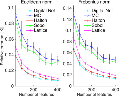
(a) USPST, $n=1506$

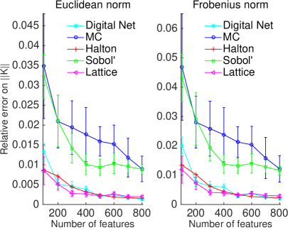
(b) cpu, $n=6554$

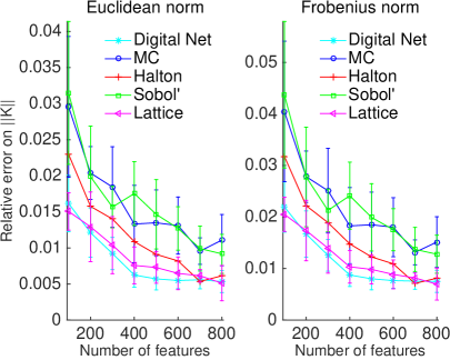
(c) census, $n=5000$

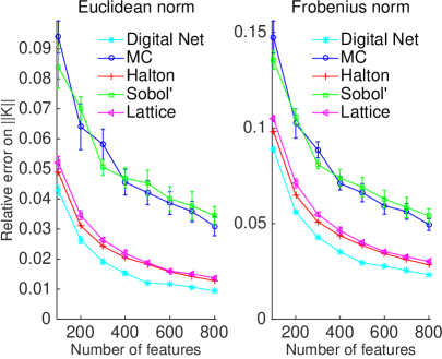
(d) MNIST, $n=5000$

Figure 2: Relative error on approximating the Gram matrix measured in Euclidean norm and Frobenius norm, i.e., $\|\mathbf{K}-\tilde{\mathbf{K}}\|_{2}/\|\mathbf{K}\|_{2}$ and $\|\mathbf{K}-\tilde{\mathbf{K}}\|_{F}/\|\mathbf{K}\|_{F}$, for various $s$. For each kind of random feature and $s$, 10 independent trials are executed, and the mean and standard deviation are plotted.

We can clearly see that except Sobol’ sequences classical low-discrepancy sequences consistently produce better approximations to the Gram matrix than the approximations produced using MC sequences. Among the four classical QMC sequences, the Digital Nets, Lattice Rules and Halton sequences yield much lower error. Similar results were observed for other datasets (not reported here). Although using scrambled variants of QMC sequences may incur some variance, the variance is quite small compared to that of the MC random features.

Scrambled (whether deterministic or randomized) QMC sequences tend to yield higher accuracies than non-scambled QMC sequences. In Figure 3, we show the ratio between the relative errors achieved by using both scrambled and non-scrambled QMC sequences. As can be seen, scrambled QMC sequences provide more accurate approximations in most cases as the ratio value tends to be less than one. In particular, scrambled Lattice sequence outperforms the non-scrambled one across all the cases for larger values of $s$. Therefore, in the rest of the experiments we use scrambled sequences.

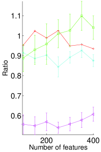
(a) USPST

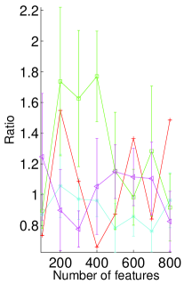
(b) CPU

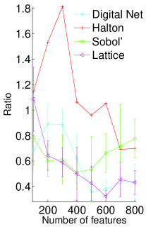
(c) CENSUS

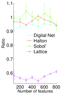
(d) MNIST

Figure 3: Ratio between relative errors on approximating the Gram matrix using both the scrambled and non-scambled version of the same QMC sequence for various $s$. The lower the ratio value is, the more accurate the scrambled QMC approximation is. For each kind of QMC sequences and $s$, $10$ independent trails are executed, and the mean and standard deviation are plotted.

Does better Gram matrix approximation translate to lower generalization errors?

We consider two regression datasets, cpu and census, and use (approximate) kernel ridge regression to build a regression model. The ridge parameter is set by the optimal value we obtain via 5-fold cross-validation on the training set by using the MC sequence. Table 1 summarizes the results.

	$s$	Halton	Sobol’	Lattice	Digit	MC
cpu	100	0.0367	0.0383	0.0374	0.0376	0.0383
		(0)	(0.0015)	(0.0010)	(0.0010)	(0.0013)
	500	0.0339	0.0344	0.0348	0.0343	0.0349
		(0)	(0.0005)	(0.0007)	(0.0005)	(0.0009)
	1000	0.0334	0.0339	0.0337	0.0335	0.0338
		(0)	(0.0007)	(0.0004)	(0.0003)	(0.0005)
census	400	0.0529	0.0747	0.0801	0.0755	0.0791
		(0)	(0.0138)	(0.0206)	(0.0080)	(0.0180)
	1200	0.0553	0.0588	0.0694	0.0587	0.0670
		(0)	(0.0080)	(0.0188)	(0.0067)	(0.0078)
	1800	0.0498	0.0613	0.0608	0.0583	0.0600
		(0)	(0.0084)	(0.0129)	(0.0100)	(0.0113)

Table 1: Regression error, i.e., $\|\hat{\mathbf{y}}-\mathbf{y}\|_{2}/\|\mathbf{y}\|_{2}$ where $\hat{\mathbf{y}}$ is the predicted value and $\mathbf{y}$ is the ground truth. For each kind of random feature and $s$, 10 independent trials are executed, and the mean and standard deviation are listed.

As we see, for cpu, all the sequences behave similarly, with the Halton sequence yielding the lowest test error. For census, the advantage of using Halton sequence is significant (almost 20% reduction in generalization error) followed by Digital Nets and Sobol’. In addition, MC sequence tends to generate higher variance across all the sampling size. Overall, QMC sequences, especially Halton, outperform MC sequences on these datasets.

When performed on classification datasets by using the same learning model, with a moderate range of $s$, e.g., less than $2000$, the QMC sequences do not yield accuracy improvements over the MC sequence with the same consistency as in the regression case. The connection between kernel approximation and the performance in downstream applications is outside the scope of the current paper. Worth mentioning in this regard, is the recent work by Bach (2013), which analyses the connection between Nyström approximations of the Gram matrix, and the regression error, and the work of El Alaoui and Mahoney (2014) on kernel methods with statistical guarantees.

Behavior of Box Discrepancy

Next, we examine if $D^{\Box}$ is predictive of the quality of approximation. We compute the normalized square box discrepancy values (i.e., $\pi^{d}(\prod^{d}_{j=1}b_{j})^{-1}D^{\Box}(S)^{2}$) as well as Gram matrix approximation error for the different sequences with different sample sizes $s$. The expected normalized square box discrepancy values for MC are computed using (13).

Our experiments revealed that using the full $\Box\mathbf{b}$ does not yield box discrepancy values that are very useful. Either the values were not predictive of the kernel approximation, or they tended to stay constant. Recall, that while the bounding box $\Box\mathbf{b}$ is set based on observed ranges of feature values in the dataset, the actual distribution of points $\bar{\mathcal{X}}$ encountered inside that box might be far from uniform. This lead us to consider the discrepancy measure when measured on the central part of the bounding box (i.e., $\Box\mathbf{b}/2$ instead of $\Box\mathbf{b}$), which is equal to the integration error averaged over that part of the bounding box. Presumably, points from $\bar{\mathcal{X}}$ concentrate in that region, and they may be more relevant for downstream predictive task.

The results are shown in Figure 4. In the top graphs we can see, as expected, increasing number of features in the sequence leads to a lower box discrepancy value. In the bottom graphs, which compare $\|\mathbf{K}-\tilde{\mathbf{K}}\|_{F}/\|\mathbf{K}\|_{F}$ to $D^{\Box\mathbf{b}/2}$, we can see a strong correlation between the quality of approximation and the discrepancy value.

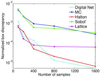
(a) cpu, $D^{\Box\mathbf{b}/2}$ versus $s$

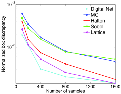
(b) census, $D^{\Box\mathbf{b}/2}$ versus $s$

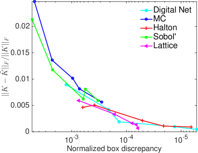
(c) cpu, relative error versus $D^{\Box\mathbf{b}/2}$

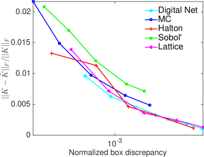
(d) census, relative error versus $D^{\Box\mathbf{b}/2}$

Figure 4: Discrepancy values ($D^{\Box\mathbf{b}/2}$) for the different sequences on cpu and census. We measure the discrepancy on the central part of the bounding box (we use $\Box\mathbf{b}/2$ instead of $\Box\mathbf{b}$ as the domain in the box discrepancy).

6.2 Experiments With Adaptive QMC

The goal of this subsection is to provide a proof-of-concept for learning adaptive QMC sequences, using the three schemes described in Section 5. We demonstrate that QMC sequences can be improved to produce better approximation to the Gram matrix, and that can sometimes lead to improved generalization error.

Note that the running time of learning the adaptive sequences is less relevant in our experimental setting for the following reasons. Given the values of $s$, $d$, $\mathbf{b}$ and $\sigma$ the optimization of a sequence needs only to be done once. There is some flexibility in these parameters: $d$ can be adjusted by adding zero features or by doing PCA on the input; one can use longer or shorter sequences; and the data can be forced to a fit a particular bounding box using (possibly non-equal) scaling of the features (this, in turn, affects the choice of the $\sigma$) . Since designing adaptive QMC sequences is data-independent with applicability to a variety of downstream applications of kernel methods, it is quite conceivable to generate many point sets in advance and to use them for many learning tasks. Furthermore, the total size of the sequences ($s\times d$) is independent of the number of examples $n$, which is the dominant term in large scale learning settings.

We name the three sequences as Global Adaptive, Greedy Adaptive and Weighted respectively. For Global Adaptive, the Halton sequence is used as the initial setting of the optimization variables $S$. For Greedy Adaptive, when optimizing for $\mathbf{w}_{t}$, the $t$-th point in the Halton sequence is used as the initial point. In both cases, we use non-linear conjugate gradient to perform numerical optimization. For Weighted, the initial features are generated using the Halton sequence and we optimize for the weights. We used CVX (Grant and Boyd, 2014, 2008) to compute the sequence (solve (17)).

Integral Approximation

We begin by examining the integration error over the unit square by using three different sequences, namely, MC, Halton and global adaptive QMC sequences. The integral is of the form $\int_{[0,1]^{2}}e^{-i\mathbf{u}^{T}\mathbf{t}}d\mathbf{t}$ where $\mathbf{u}$ spans the unit square. The error is plotted in Figure 5. We see that MC sequences concentrate most of the error reduction near the origin. The Halton sequence gives significant improvement expanding the region of low integration error. Global adaptive QMC sequences give another order of magnitude improvement in integration error which is now diffused over the entire unit square; the estimation of such sequences is “aware” of the full integration region. In fact, by controlling the box size (see plot labeled b/2), adaptive sequences can be made to focus in a specified sub-box which can help with generalization if the actual data distribution is better represented by this sub-box.

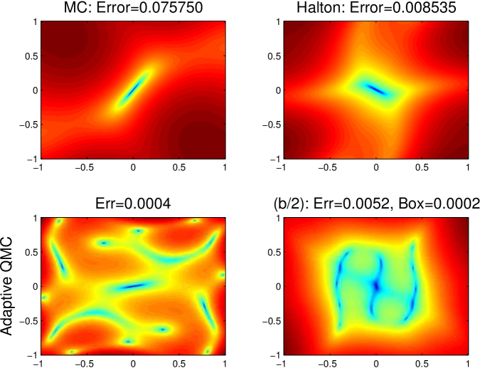
Figure 5: Integration error.

Quality of Kernel Approximation

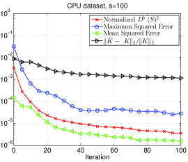
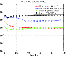
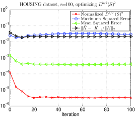
(a)	(b)	(c)

Figure 6: Examining the behavior of learning Global Adaptive sequences. Various metrics on the Gram matrix approximation are plotted.

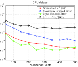
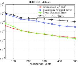
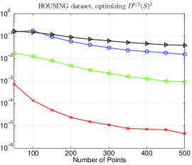
(a)	(b)	(c)

Figure 7: Examining the behavior of learning Greedy Adaptive sequences. Various metrics on the Gram matrix approximation are plotted.

In Figure 6 and Figure 7 we examine how various metrics (discrepancy, maximum squared error, mean squared error, norm of the error) on the Gram matrix approximation evolve during the optimization process for both adaptive sequences. Since learning the adaptive sequences on dataset with low dimensional features is more affordable, the experiment is performed on two such datasets, namely, cpu and housing.

For Global Adaptive, we fixed $s=100$ and examine how the performance evolves as the number of iterations grows. In Figure 6 (a) we examine the behavior on cpu. We see that all metrics go down as the iteration progresses. This supports our hypothesis that by optimizing the box discrepancy we can improve the approximation of the Gram matrix. Figure 6 (b), which examines the same metrics on the scaled version of the housing dataset, has some interesting behaviors. Initially all metrics go down, but eventually all the metrics except the box-discrepancy start to go up; the box-discrepancy continues to go down. One plausible explanation is that the integrands are not uniformly distributed in the bounding box, and that by optimizing the expectation over the entire box we start to overfit it, thereby increasing the error in those regions of the box where integrands actually concentrate. One possible way to handle this is to optimize closer to the center of the box (e.g., on $\Box\mathbf{b}/2$), under the assumption that integrands concentrate there. In Figure 6 (c) we try this on the housing dataset. We see that now the mean error and the norm error are much improved, which supports the interpretation above. But the maximum error eventually goes up. This is quite reasonable as the outer parts of the bounding box are harder to approximate, so the maximum error is likely to originate from there. Subsequently, we stop the adaptive learning of the QMC sequences early, to avoid the actual error from going up due to averaging.

For Greedy Adaptive, we examine its behavior as the number of points increases. In Figure 7 (a) and (b), as expected, as the number of points in the sequence increases, the box discrepancy goes down. This is also translated to non-monotonic decrease in the other metrics of Gram matrix approximation. However, unlike the global case, we see in Figure 7 (c), when the points are generated by optimizing on a smaller box $\Box\mathbf{b}/2$, the resulting metrics become higher for a fixed number of points. Although the Greedy Adaptive sequence can be computed faster than the adaptive sequence, potentially it might need a large number of points to achieve certain low magnitude of discrepancy. Hence, as shown in the plots, when the number of points is below 500, the quality of the optimization is not good enough to provide a good approximation the Gram matrix. For example, one can check when the number of points is 100, the discrepancy value of the Greedy Adaptive sequence is higher than that of the Global Adaptive sequence with more than 10 iterations.

		$D^{\Box\mathbf{b}}$				$D^{\Box\mathbf{b}/4}$
	$s$	Halton	Globalb	Greedyb	Weightedb	Halton	Globalb/4	Greedyb/4	Weightedb/4
cpu	100	3.41e-3	1.29e-6	3.02e-4	7.84e-5	9.44e-5	5.57e-8	2.62e-5	1.67e-8
	300	8.09e-4	5.14e-6	5.85e-5	1.45e-6	2.57e-5	1.06e-7	3.08e-6	2.93e-9
	500	2.39e-4	2.83e-6	1.86e-5	3.39e-7	7.91e-6	2.62e-8	1.04e-6	2.43e-9
census	400	2.61e-3	9.32e-4	7.47e-4	8.83e-4	5.73e-4	2.79e-5	2.20e-5	2.45e-5
	800	1.21e-3	5.02e-4	3.33e-4	4.91e-4	2.21e-4	1.12e-5	8.04e-6	5.46e-6
	1200	8.27e-4	3.41e-4	2.06e-4	3.39e-4	1.39e-4	8.15e-6	4.23e-6	2.29e-6
	1800	5.31e-4	2.17e-4	1.27e-4	2.31e-4	3.79e-5	5.59e-6	2.63e-6	8.37e-7
	2200	4.33e-4	1.73e-4	1.01e-4	1.87e-4	2.34e-5	3.35e-6	1.95e-6	4.93e-7

Table 2: Discrepancy values, measured on the full bounding box and its central part, i.e., $D^{\Box\mathbf{b}}$ and $D^{\Box\mathbf{b}/4}$.

Table 2 also shows the discrepancy values of various sequences on cpu and census. Using adaptive sequences improves the discrepancy values by orders-of-magnitude. We note that a significant reduction in terms of discrepancy values can be achieved using only weights, sometimes yielding discrepancy values that are better than the hard-to-compute global or greedy sequences.

Generalization Error

We use the three algorithms for learning adaptive sequences as described in the previous subsections, and use them for doing approximate kernel ridge regression. The ridge parameter is set by the value which is near-optimal for both sequences in 5-fold cross-validation on the training set. Table 3 summarizes the results.

	$s$	Halton	Globalb	Globalb/4	Greedyb	Greedyb/4	Weightedb	Weightedb/4
cpu	100	0.0304	0.0315	0.0296	0.0307	0.0296	0.0366	0.0305
	300	0.0303	0.0278	0.0293	0.0274	0.0269	0.0290	0.0302
	500	0.0348	0.0347	0.0348	0.0328	0.0291	0.0342	0.0347
census	400	0.0529	0.1034	0.0997	0.0598	0.0655	0.0512	0.0926
	800	0.0545	0.0702	0.0581	0.0522	0.0501	0.0476	0.0487
	1200	0.0553	0.0639	0.0481	0.0525	0.0498	0.0496	0.0501
	1800	0.0498	0.0568	0.0476	0.0685	0.0548	0.0498	0.0491
	2200	0.0519	0.0487	0.0515	0.0694	0.0504	0.0529	0.0499

Table 3: Regression error, i.e., $\|\hat{\mathbf{y}}-\mathbf{y}\|_{2}/\|\mathbf{y}\|_{2}$ where $\hat{\mathbf{y}}$ is the predicted value and $\mathbf{y}$ is the ground truth.

For both cpu and census, at least one of the adaptive sequences sequences can yield lower test error for each sampling size (since the test error is already low, around 3% or 5%, such improvement in accuracy is not trivial). For cpu, greedy approach seems to give slightly better results. When $s=500$ or even larger (not reported here), the performance of the sequences are very close. For census, the weighted sequence yields the lowest generalization error when $s=400,800$. Afterwards we can see global adaptive sequence outperforms the rest of the sequences, even though it has better discrepancy values. In some cases, adaptive sequences sometimes produce errors that are bigger than the unoptimized sequences.

In most cases, the adaptive sequence on the central part of the bounding box outperforms the adaptive sequence on the entire box. This is likely due to the non-uniformity phenomena discussed earlier.

7 Conclusion and Future Work

Recent work on applying kernel methods to very large datasets, has shown their ability to achieve state-of-the-art accuracies that sometimes match those attained by Deep Neural Networks (DNN) (Huang et al., 2014). Key to these results is the ability to apply kernel method to such datasets. The random features approach, originally due to Rahimi and Recht (2008), as emerged as a key technology for scaling up kernel methods (Sindhwani and Avron, 2014).

Close examination of those empirical results reveals that to achieve state-of-the-art accuracies, a very large number of random features was needed. For example, on TIMIT, a classical speech recognition dataset, over 200,000 random features were used in order to match DNN performance (Huang et al., 2014). It is clear that improving the efficiency of random features can have a significant impact on our ability to scale up kernel methods, and potentially get even higher accuracies.

This paper is the first to exploit high-dimensional approximate integration techniques from the QMC literature in this context, with promising empirical results backed by rigorous theoretical analyses. Avenues for future work include incorporating stronger data-dependence in the estimation of adaptive sequences and analyzing how resulting Gram matrix approximations translate into downstream performance improvements for a variety of large-scale learning tasks.

Appendix A Technical Details

In this section we give detailed proofs of the assertions made in Section 4 and 5.

A.1 Proof of Proposition 5

Recall, for any $\mathbf{t}\in\mathbb{R}^{d}$, for $\Phi^{-1}(\mathbf{t})$, we mean $\left(\Phi_{1}^{-1}(t_{1}),\ldots,\Phi_{d}^{-1}(t_{d})\right)\in\mathbb{R}^{d}$, where $\Phi_{j}(\cdot)$ is the CDF of $p_{j}(\cdot)$.

From $f_{\mathbf{u}}(\mathbf{t})=e^{-i\mathbf{u}^{T}\Phi^{-1}(\mathbf{t})}$, for any $j=1,\ldots,d$, we have

$$\frac{\partial f(\mathbf{t})}{\partial\mathbf{t}_{j}}=(-i)\frac{u_{j}}{p_{j}(\Phi_{j}^{-1}(t_{j}))}e^{-i\mathbf{u}^{T}\Phi_{j}^{-1}(\mathbf{t})}~{}.$$

Thus,

$$\frac{\partial^{d}f(\mathbf{t})}{\partial t_{1}\cdots\partial t_{d}}=\prod_{j=1}^{d}\left((-i)\frac{u_{j}}{p_{j}(\Phi_{j}^{-1}(t_{j}))}\right)e^{-i\mathbf{u}^{T}\Phi_{j}^{-1}(\mathbf{t})}~{}.$$

In (6), when $I=[d]$,

$$\int_{[0,1]^{|I|}}\left|\frac{\partial f}{\partial\mathbf{u}_{I}}\right|d\mathbf{t}_{I} = \int_{[0,1]^{d}}\left|\frac{\partial^{d}f(\mathbf{t})}{\partial t_{1}\cdots\partial t_{d}}\right|dt_{1}\cdots dt_{d}$$ (18)

$$= \int_{[0,1]^{d}}\left|\prod_{j=1}^{d}\left((-i)\frac{u_{j}}{p_{j}(\Phi_{j}^{-1}(t_{j}))}\right)e^{-i\mathbf{u}^{T}\Phi_{j}^{-1}(\mathbf{t})}\right|dt_{1}\cdots dt_{d}$$

$$= \int_{[0,1]^{d}}\prod_{j=1}^{d}\left|\frac{u_{j}}{p_{j}(\Phi_{j}^{-1}(t_{j}))}\right|dt_{1}\cdots dt_{d}$$

$$= \prod_{j=1}^{d}\left(\int_{[0,1]}\left|\frac{u_{j}}{p_{j}(\Phi_{j}^{-1}(t_{j}))}\right|dt_{j}\right)~{}.$$

With a change of variable, $\Phi_{j}(t_{j})=v_{j}$, for $j=1,\ldots,d$, (18) becomes

$$\prod_{j=1}^{d}\left(\int_{[0,1]}\left|\left(\frac{u_{j}}{p_{j}(\Phi_{j}^{-1}(t_{j}))}\right)\right|dt_{j}\right)=\prod_{j=1}^{d}\left(\int_{\mathbb{R}}|u_{j}|dv_{j}\right)=\infty~{}.$$

As this is a term in (6), we know that $V_{HK}[f_{\mathbf{u}}(\mathbf{t})]$ is unbounded.

A.2 Proof of Proposition 6

We need the following lemmas, across which we share some notation.

Lemma 17.

Assuming that $\kappa=\sup_{\mathbf{x}\in\mathbb{R}^{d}}h(\mathbf{x},\mathbf{x})<\infty$, if $f\in\mathcal{H}$, where $\mathcal{H}$ is an RKHS with kernel $h(\cdot,\cdot)$, the integral $\int_{\mathbb{R}^{d}}f(\mathbf{x})p(\mathbf{x})d\mathbf{x}$ is finite.

Proof.

For notational convenience, we note that

$$\int_{\mathbb{R}^{d}}f(\mathbf{x})p(\mathbf{x})d\mathbf{x}=\mbox{}{\mathbb{E}}\left[f(X)\right],$$

where $\mbox{}{\mathbb{E}}\left[\cdot\right]$ denotes expectation and $X$ is a random variable distributed according to the probability density $p(\cdot)$ on $\mathbb{R}^{d}$.

Now consider a linear functional $T$ that maps $f$ to $\mbox{}{\mathbb{E}}\left[f(X)\right]$, i.e.,

$$T[f]=\mbox{}{\mathbb{E}}\left[f(X)\right].$$ (19)

The linear functional $T$ is a bounded linear functional on the RKHS $\mathcal{H}$. To see this:

$$|\mbox{}{\mathbb{E}}\left[f(X)\right]| \leq \mbox{}{\mathbb{E}}\left[|f(X)|\right]~{}~{}~{}~{}\textrm{(Jensen's Inequality)}$$

$$= \mbox{}{\mathbb{E}}\left[|\langle f,h(X,\cdot)\rangle_{\mathcal{H}}|\right]~{}~{}~{}~{}\textrm{(Reproducing Property)}$$

$$\leq \|f\|_{\mathcal{H}}\mbox{}{\mathbb{E}}\left[\|h(X,\cdot)\|_{\mathcal{H}}\right]~{}~{}~{}~{}\textrm{(Cauchy-Schwartz)}$$

$$\leq \|f\|_{\mathcal{H}}\mbox{}{\mathbb{E}}\left[\sqrt{h(X,X)}\right]=\|f\|_{\mathcal{H}}\sqrt{\kappa}<\infty~{}.$$

This shows that the integral $\int_{\mathbb{R}^{d}}f(\mathbf{x})p(\mathbf{x})d\mathbf{x}$ exists. ∎

Lemma 18.

The mean $\mu_{h,p}(\mathbf{u})=\int_{\mathbb{R}^{d}}h(\mathbf{u},\mathbf{x})p(\mathbf{x})d\mathbf{x}$ is in $\mathcal{H}$. In addition, for any $f\in\mathcal{H}$,

$$\mbox{}{\mathbb{E}}\left[f(X)\right]=\int_{\mathbb{R}^{d}}f(\mathbf{x})p(\mathbf{x})d\mathbf{x}=\langle f,\mu_{h,p}\rangle_{\mathcal{H}}~{}.$$ (20)

Proof.

From the Riesz Representation Theorem, every bounded linear functional on $\mathcal{H}$ admits an inner product representation. Therefore, for $T$ defined in (19), there exists $\mu_{h,p}\in\mathcal{H}$ such that,

$$T[f]=\mbox{}{\mathbb{E}}\left[f(X)\right]=\langle f,\mu_{h,p}\rangle_{\mathcal{H}}~{}.$$

Therefore we have, $\langle f,\mu_{h,p}\rangle_{\mathcal{H}}=\int f(\mathbf{x})p(\mathbf{x})d\mathbf{x}$ for all $f\in\mathcal{H}$. For any $\mathbf{z}$, choosing $f(\cdot)=h(\mathbf{z},\cdot)$, where $h(\cdot,\cdot)$ is the kernel associated with $\mathcal{H}$, and invoking the reproducing property we see that,

$$\mu_{h,p}(\mathbf{z})=\langle h(\mathbf{z},\cdot),\mu_{h,p}\rangle_{\mathcal{H}}=\int_{\mathbb{R}^{d}}h(\mathbf{z},\mathbf{x})p(\mathbf{x})d\mathbf{x}~{}.$$

∎

The proof of Proposition 6 follows from the existence Lemmas above, and the following steps.

$$\epsilon_{S,p}[f] = \left|\int_{\mathbb{R}^{d}}f(\mathbf{x})p(\mathbf{x})d\mathbf{x}-\frac{1}{s}\sum_{l=1}^{s}f(\mathbf{w}_{l})\right|$$

$$= \left|\langle f,\mu_{h,p}\rangle_{\mathcal{H}}-\frac{1}{s}\sum_{l=1}^{s}\langle f,h(\mathbf{w}_{l},\cdot)\rangle_{\mathcal{H}}\right|$$

$$= \left|\langle f,\mu_{h,p}-\frac{1}{s}\sum_{l=1}^{s}h(\mathbf{w}_{l},\cdot)\rangle_{\mathcal{H}}\right|$$

$$\leq \left\|f\right\|_{\mathcal{H}}\left\|\mu_{h,p}-\frac{1}{s}\sum_{l=1}^{s}h(\mathbf{w}_{l},\cdot)\right\|_{\mathcal{H}}=\left\|f\right\|_{\mathcal{H}}D_{h,p}(S)~{},$$

where $D_{h,p}(S)$ is given as follows,

$$D_{h,p}(S)^{2} = \left\|\mu_{h,p}-\frac{1}{s}\sum_{l=1}^{s}h(\mathbf{w}_{l},\cdot)\right\|^{2}_{\mathcal{H}}$$

$$= \langle\mu_{h,p},\mu_{h,p}\rangle_{\mathcal{H}}-\frac{2}{s}\sum_{l=1}^{s}\langle\mu_{h,p},h(\mathbf{w}_{l},\cdot)\rangle_{\mathcal{H}}+\frac{1}{s^{2}}\sum_{l=1}^{s}\sum_{j=1}^{s}\langle h(\mathbf{w}_{l},\cdot),h(\mathbf{w}_{j},\cdot)\rangle_{\mathcal{H}}$$

$$= \mbox{}{\mathbb{E}}\left[\mu_{h,p}(X)\right]-\frac{2}{s}\sum_{l=1}^{s}\mbox{}{\mathbb{E}}\left[h(\mathbf{w}_{l},\cdot)\right]+\frac{1}{s^{2}}\sum_{l=1}^{s}\sum_{j=1}^{s}h(\mathbf{w}_{l},\mathbf{w}_{j})$$

$$= \int_{\mathbb{R}^{d}}\int_{\mathbb{R}^{d}}h(\omega,\phi)p(\omega)p(\phi)d\omega d\phi-\frac{2}{s}\sum^{s}_{l=1}\int_{\mathbb{R}^{d}}h(\mathbf{w}_{l},\omega)p(\omega)d\omega$$

$$\qquad+\frac{1}{s^{2}}\sum_{l=1}^{s}\sum_{j=1}^{s}h(\mathbf{w}_{l},\mathbf{w}_{j})~{}.$$

A.3 Proof of Theorem 9

We apply (6) to the particular case of $h=\operatorname{sinc}_{\mathbf{b}}$. We have

$$\int_{\mathbb{R}^{d}}\int_{\mathbb{R}^{d}}h(\omega,\phi)p(\omega)p(\phi)d\omega d\phi = \pi^{-d}\int_{\mathbb{R}^{d}}\int_{\mathbb{R}^{d}}\prod^{d}_{j=1}\frac{\sin(b_{j}(\omega_{j}-\phi_{j}))}{\omega_{j}-\phi_{j}}p_{j}(\omega_{j})p_{j}(\phi_{j})d\omega d\phi$$

$$= \pi^{-d}\prod^{d}_{j=1}\int_{\mathbb{R}}\int_{\mathbb{R}}\frac{\sin(b_{j}(\omega_{j}-\phi_{j}))}{\omega_{j}-\phi_{j}}p_{j}(\omega_{j})p_{j}(\phi_{j})d\omega_{j}d\phi_{j}~{},$$

and

$$\sum^{s}_{l=1}\int_{\mathbb{R}^{d}}h(w_{l},\omega)p(\omega)d\omega = \pi^{-d}\sum^{s}_{l=1}\int_{\mathbb{R}^{d}}\prod^{d}_{j=1}\frac{\sin(b_{j}(w_{lj}-\omega_{j}))}{w_{lj}-\omega_{j}}p_{j}(\omega_{j})d\omega$$

$$= \pi^{-d}\sum^{s}_{l=1}\prod^{d}_{j=1}\int_{\mathbb{R}^{d}}\frac{\sin(b_{j}(w_{lj}-\omega_{j}))}{w_{lj}-\omega_{j}}p_{j}(\omega_{j})d\omega_{j}~{}.$$

So we can consider each coordinate on its own.

Fix $j$. We have

$$\int_{\mathbb{R}}\frac{\sin(b_{j}x)}{x}p_{j}(x)dx = \int_{\mathbb{R}}\int_{0}^{b_{j}}\cos(\beta x)p_{j}(x)d\beta dx$$

$$= \frac{1}{2}\int_{-b_{j}}^{b_{j}}\int_{\mathbb{R}}e^{i\beta x}p(x)dxd\beta$$

$$= \frac{1}{2}\int_{-b_{j}}^{b_{j}}\varphi_{j}(\beta)d\beta~{}.$$

The interchange in the second line is allowed since the $p_{j}(x)$ makes the function integrable (with respect to $x$).

Now fix $w\in\mathbb{R}$ as well. Let $h_{j}(x,y)=\sin(b_{j}(x-y))/\pi(x-y)$. We have

$$\int_{\mathbb{R}}h_{j}(\omega,w)p_{j}(\omega)d\omega = \pi^{-1}\int_{\mathbb{R}}\frac{\sin(b_{j}(\omega-w))}{\omega-w}p_{j}(\omega)d\omega$$

$$= \pi^{-1}\int_{\mathbb{R}}\frac{\sin(b_{j}x)}{x}p_{j}(x+w)dx$$

$$= (2\pi)^{-1}\int_{-b_{j}}^{b_{j}}\varphi_{j}(\beta)e^{iw\beta}d\beta~{},$$

where the last equality follows from first noticing that the characteristic function associated with the density function $x\mapsto p_{j}(x+w)$ is $\beta\mapsto\varphi(\beta)e^{iw\beta}$, and then applying the previous inequality.

We also have,

$$\int_{\mathbb{R}}\int_{\mathbb{R}}\frac{\sin(b_{j}(x-y))}{x-y}p_{j}(x)p_{j}(y)dxdy = \int_{\mathbb{R}}\int_{\mathbb{R}}\int_{0}^{b_{j}}\cos(\beta(x-y))p_{j}(x)p_{j}(y)d\beta dxdy$$

$$= \frac{1}{2}\int_{\mathbb{R}}\int_{\mathbb{R}}\int_{-b_{j}}^{b_{j}}e^{i\beta(x-y)}p_{j}(x)p_{j}(y)d\beta dxdy$$

$$= \frac{1}{2}\int_{-b_{j}}^{b_{j}}\int_{\mathbb{R}}\int_{\mathbb{R}}e^{i\beta(x-y)}p_{j}(x)p_{j}(y)dxdyd\beta$$

$$= \frac{1}{2}\int_{-b_{j}}^{b_{j}}\left(\int_{\mathbb{R}}e^{i\beta x}p_{j}(x)dx\right)\left(\int_{\mathbb{R}}e^{-i\beta y}p_{j}(y)dy\right)d\beta$$

$$= \frac{1}{2}\int_{-b_{j}}^{b_{j}}\varphi_{j}(\beta)\varphi_{j}(\beta)^{*}d\beta$$

$$= \frac{1}{2}\int_{-b_{j}}^{b_{j}}\lvert\varphi_{j}(\beta)\rvert^{2}d\beta~{}.$$

The interchange at the third line is allowed because of $p_{j}(x)p_{j}(y)$. In the last line we use the fact that the $\varphi_{j}(\cdot)$ is Hermitian.

A.4 Proof of Theorem 12

Let $b>0$ be a scalar, and let $u\in[-b,b]$ and $z\in\mathbb{R}$. We have,

$$\int^{\infty}_{-\infty}e^{-iux}\frac{\sin(b(x-z))}{\pi(x-z)}dx = e^{-iuz}\int^{\infty}_{-\infty}e^{-i2\pi\frac{u}{2b}y}\frac{\sin(\pi y)}{\pi y}dy$$

$$= e^{-iuz}\operatorname{rect}(u/2b)$$

$$= e^{-iuz}~{}.$$

In the above, $\operatorname{rect}$ is the function that is 1 on $[-1/2,1/2]$ and zero elsewhere.

The last equality implies that for every $\mathbf{u}\in\Box\mathbf{b}$ and every $\mathbf{x}\in\mathbb{R}^{d}$ we have

$$f_{\mathbf{u}}(\mathbf{x})=\int_{\mathbb{R}^{d}}f_{\mathbf{u}}(\mathbf{y})\operatorname{sinc}_{\mathbf{b}}(\mathbf{y},\mathbf{x})d\mathbf{y}~{}.$$

We now have for every $\mathbf{u}\in\Box\mathbf{b}$,

$$\epsilon_{S,p}[f_{\mathbf{u}}] = \left|\int_{\mathbb{R}^{d}}f_{\mathbf{u}}(\mathbf{x})p(\mathbf{x})d\mathbf{x}-\frac{1}{s}\sum_{i=1}^{s}f(\mathbf{w}_{i})\right|$$

$$= \left|\int_{\mathbb{R}^{d}}\int_{\mathbb{R}^{d}}f_{\mathbf{u}}(\mathbf{y})\operatorname{sinc}_{\mathbf{b}}(\mathbf{y},\mathbf{x})d\mathbf{y}p(\mathbf{x})d\mathbf{x}-\frac{1}{s}\sum_{i=1}^{s}\int_{\mathbb{R}^{d}}f_{\mathbf{u}}(\mathbf{y})\operatorname{sinc}_{\mathbf{b}}(\mathbf{y},\mathbf{w}_{i})d\mathbf{y}\right|$$

$$= \left|\int_{\mathbb{R}^{d}}f_{\mathbf{u}}(\mathbf{y})\left[\int_{\mathbb{R}^{d}}\operatorname{sinc}_{\mathbf{b}}(\mathbf{y},\mathbf{x})p(\mathbf{x})d\mathbf{x}-\frac{1}{s}\sum_{i=1}^{s}\operatorname{sinc}_{\mathbf{b}}(\mathbf{y},\mathbf{w}_{i})\right]d\mathbf{y}\right|~{}.$$

Let us denote

$$r_{S}(\mathbf{y})=\int_{\mathbb{R}^{d}}\operatorname{sinc}_{\mathbf{b}}(\mathbf{y},\mathbf{x})p(\mathbf{x})d\mathbf{x}-\frac{1}{s}\sum_{i=1}^{s}\operatorname{sinc}_{\mathbf{b}}(\mathbf{y},\mathbf{w}_{i})~{}.$$

So,

$$\epsilon_{S,p}[f_{\mathbf{u}}]=\left|\int_{\mathbb{R}^{d}}f_{\mathbf{u}}(\mathbf{y})r_{S}(\mathbf{y})d\mathbf{y}\right|~{}.$$

The function $r_{S}(\cdot)$ is square-integrable, so it has a Fourier transform $\hat{r}_{S}(\cdot)$. The above formula is exactly the value of $\hat{r}_{S}(\mathbf{u})$. That is,

$$\epsilon_{S,p}[f_{\mathbf{u}}]=\left|\hat{r}_{S}(\mathbf{u})\right|~{}.$$

Now,

$$\mbox{}{\mathbb{E}}_{f\sim{\cal U}(\mathcal{F}_{\Box\mathbf{b}})}\left[\epsilon_{S,p}[f]^{2}\right] = \mbox{}{\mathbb{E}}_{\mathbf{u}\sim{\cal U}(\Box\mathbf{b})}\left[\epsilon_{S,p}[f_{\mathbf{u}}]^{2}\right]$$

$$= \int_{\mathbf{u}\in\Box\mathbf{b}}\left|\hat{r}_{S}(\mathbf{u})\right|^{2}\left(\prod^{d}_{j=1}2b_{j}\right)^{-1}d\mathbf{u}$$

$$= \left(\prod^{d}_{j=1}2b_{j}\right)^{-1}\|\hat{r}_{S}\|^{2}_{L2}$$

$$= \frac{(2\pi)^{d}}{\prod^{d}_{j=1}2b_{j}}\|r_{S}\|^{2}_{PW_{\mathbf{b}}}$$

$$= \frac{\pi^{d}}{\prod^{d}_{j=1}b_{j}}D^{\Box}_{p}(S)^{2}~{}.$$

The equality before the last follows from Plancherel formula and the equality of the norm in $PW_{\mathbf{b}}$ to the $L2$-norm. The last equality follows from the fact that $r_{S}$ is exactly the expression used in the proof of Proposition 6 to derive $D^{\Box}_{p}$.

A.5 Proof of Corollary 13

In this case, $p(\mathbf{x})=\prod_{j=1}^{d}p_{j}(x_{j})$ where $p_{j}(\cdot)$ is the density function of $\mathcal{N}(0,1/\sigma_{j})$. The characteristic function associated with $p_{j}(\cdot)$ is $\varphi_{j}(\beta)=e^{-\frac{\beta^{2}}{2\sigma_{j}^{2}}}$. We apply (11) directly.

For the first term, since

$$\int_{0}^{b_{j}}\lvert\varphi_{j}(\beta)\rvert^{2}d\beta = \int_{0}^{b_{j}}e^{-\frac{\beta^{2}}{\sigma_{j}^{2}}}d\beta$$

$$= \sigma_{j}\int_{0}^{b_{j}/\sigma_{j}}e^{-y^{2}}dy$$

$$= \frac{\sigma_{j}\sqrt{\pi}}{2}\operatorname{erf}\left(\frac{b_{j}}{\sigma_{j}}\right)~{},$$

we have

$$\pi^{-d}\prod_{j=1}^{d}\int_{0}^{b_{j}}\lvert\varphi_{j}(\beta)\rvert^{2}d\beta=\prod_{j=1}^{d}\frac{\sigma_{j}}{2\sqrt{\pi}}\operatorname{erf}\left(\frac{b_{j}}{\sigma_{j}}\right)~{}.$$ (21)

For the second term, since

$$\int_{-b_{j}}^{b_{j}}\varphi_{j}(\beta)e^{iw_{lj}\beta}d\beta = \int_{-b_{j}}^{b_{j}}e^{-\frac{\beta_{j}^{2}}{2\sigma^{2}}+iw_{lj}\beta}d\beta$$

$$= e^{-\frac{\sigma_{j}w_{lj}}{2}}\int_{-b_{j}}^{b_{j}}e^{-\left(\frac{\beta}{\sqrt{2}\sigma_{j}}-i\frac{\sigma_{j}w_{lj}}{\sqrt{2}}\right)^{2}}d\beta$$

$$= \sqrt{2}\sigma_{j}e^{-\frac{\sigma_{j}^{2}w_{lj}^{2}}{2}}\int_{-\frac{b_{j}}{\sqrt{2}\sigma_{j}}}^{\frac{b_{j}}{\sqrt{2}\sigma_{j}}}e^{-\left(y-i\frac{\sigma_{j}w_{lj}}{\sqrt{2}}\right)^{2}}dy$$

$$= \sqrt{2}\sigma_{j}e^{-\frac{\sigma_{j}^{2}w_{lj}^{2}}{2}}\int_{-\frac{b_{j}}{\sqrt{2}\sigma_{j}}-i\frac{\sigma_{j}w_{lj}}{\sqrt{2}}}^{\frac{b_{j}}{\sqrt{2}\sigma_{j}}-i\frac{\sigma_{j}w_{lj}}{\sqrt{2}}}e^{-z^{2}}dz$$

$$= \frac{\sqrt{\pi}\sigma_{j}}{\sqrt{2}}e^{-\frac{\sigma_{j}^{2}w_{lj}^{2}}{2}}\left(\operatorname{erf}\left(-\frac{b_{j}}{\sqrt{2}\sigma_{j}}-i\frac{\sigma_{j}w_{lj}}{\sqrt{2}}\right)-\operatorname{erf}\left(\frac{b_{j}}{\sqrt{2}\sigma_{j}}-i\frac{\sigma_{j}w_{lj}}{\sqrt{2}}\right)\right)$$

$$= \sqrt{2\pi}\sigma_{j}e^{-\frac{\sigma_{j}^{2}w_{lj}^{2}}{2}}\operatorname{Re}\left(\operatorname{erf}\left(-\frac{b_{j}}{\sqrt{2}\sigma_{j}}-i\frac{\sigma_{j}w_{lj}}{\sqrt{2}}\right)\right)~{},$$

we have

$$\frac{2}{s}(2\pi)^{-d}\sum_{l=1}^{s}\prod_{j=1}^{d}\int_{-b_{j}}^{b_{j}}\varphi_{j}(\beta)e^{i\mathbf{w}_{lj}\beta}d\beta=\frac{2}{s}\sum_{l=1}^{s}\prod_{j=1}^{d}\frac{\sigma_{j}}{\sqrt{2\pi}}e^{-\frac{\sigma_{j}^{2}w_{lj}^{2}}{2}}\operatorname{Re}\left(\operatorname{erf}\left(-\frac{b_{j}}{\sqrt{2}\sigma_{j}}-i\frac{\sigma_{j}w_{lj}}{\sqrt{2}}\right)\right)~{}.$$ (22)

Combining (21), (22) and (11), (12) follows.

A.6 Proof of Corollary 14

The proof is similar to the proof of Theorem 3.6 of Dick et al. (2013). Notice that since $\sup_{\mathbf{x}\in\mathbb{R}^{d}}h(\mathbf{x},\mathbf{x})<\infty$, we have $\int_{\mathbb{R}^{d}}h(\mathbf{x},\mathbf{x})p(\mathbf{x})d\mathbf{x}<\infty$. From Lemma 18 we know that $\int_{\mathbb{R}^{d}}h(\cdot,\mathbf{y})p(\mathbf{y})d\mathbf{y}\in\mathcal{H}$, hence from Lemma 17, we have $\int_{\mathbb{R}^{d}}\int_{\mathbb{R}^{d}}h(\mathbf{x},\mathbf{y})p(\mathbf{x})p(\mathbf{y})d\mathbf{x}d\mathbf{y}<\infty$.

By (6), we have

$$D_{h,p}(S)^{2} = \int_{\mathbb{R}^{d}}\int_{\mathbb{R}^{d}}h(\omega,\phi)p(\omega)p(\phi)d\omega d\phi$$

$$-\frac{2}{s}\sum^{s}_{l=1}\int_{\mathbb{R}^{d}}h(\mathbf{w}_{l},\omega)p(\omega)d\omega$$

$$+\frac{1}{s^{2}}\sum_{l=1}^{s}h(\mathbf{w}_{l},\mathbf{w}_{l})+\frac{1}{s^{2}}\sum_{l,j=1,l\neq j}^{s}h(\mathbf{w}_{l},\mathbf{w}_{j})~{}.$$

Then,

$$\begin{split}\mbox{}{\mathbb{E}}\left[D_{h,p}(S)^{2}\right]=\int_{[0,1]^{d}}\cdots\int_{[0,1]^{d}}\left(\int_{\mathbb{R}^{d}}\int_{\mathbb{R}^{d}}h(\omega,\phi)p(\omega)p(\phi)d\omega d\phi-\frac{2}{s}\sum^{s}_{l=1}\int_{\mathbb{R}^{d}}h(\Phi^{-1}(\mathbf{t}_{l}),\omega)p(\omega)d\omega\right.\\ \left.+\frac{1}{s^{2}}\sum_{l=1}^{s}h(\Phi^{-1}(\mathbf{t}_{l}),\Phi^{-1}(\mathbf{t}_{l}))+\frac{1}{s^{2}}\sum_{l,j=1,l\neq j}^{s}h(\Phi^{-1}(\mathbf{t}_{l}),\Phi^{-1}(\mathbf{t}_{j}))\right)d\mathbf{t}_{1}\cdots d\mathbf{t}_{s}~{}.\end{split}$$

Obviously, the first is a constant which is independent to $\mathbf{t}_{1},\ldots,\mathbf{t}_{s}$. Since all the terms are finite, we can interchange the integral and the sum among rest terms. In the second term, for each $l$, the only dependence on $\mathbf{t}_{1},\ldots,\mathbf{t}_{s}$ is $\mathbf{t}_{l}$, hence all the other $\mathbf{t}_{j}$ can be integrated out. That is,

$$\int_{[0,1]^{d}}\cdots\int_{[0,1]^{d}}\int_{\mathbb{R}^{d}}h(\Phi^{-1}(\mathbf{t}_{l}),\omega)p(\omega)d\omega d\mathbf{t}_{1}\cdots d\mathbf{t}_{s} = \int_{[0,1]^{d}}\int_{\mathbb{R}^{d}}h(\Phi^{-1}(\mathbf{t}_{l}),\omega)p(\omega)d\omega d\mathbf{t}_{l}$$

$$= \int_{\mathbb{R}^{d}}\int_{\mathbb{R}^{d}}h(\phi,\omega)p(\phi)p(\omega)d\phi d\omega.$$

Above, the last equality comes from a change of variable, i.e., $\mathbf{t}_{l}=\left(\Phi_{1}(\phi_{1}),\ldots,\Phi_{d}(\phi_{d})\right)$.

Similar operations can be done for the third and fourth term. Combining all of these, we have the following,

$$\mbox{}{\mathbb{E}}\left[D_{h,p}(S)^{2}\right] = \int_{\mathbb{R}^{d}}\int_{\mathbb{R}^{d}}h(\omega,\phi)p(\omega)p(\phi)d\omega d\phi-2\int_{\mathbb{R}^{d}}\int_{\mathbb{R}^{d}}h(\omega,\phi)p(\omega)p(\phi)d\omega d\phi$$

$$+\frac{1}{s}\int_{\mathbb{R}^{d}}h(\omega,\omega)p(\omega)d\omega+\frac{s-1}{s}\int_{\mathbb{R}^{d}}\int_{\mathbb{R}^{d}}h(\omega,\phi)p(\omega)p(\phi)d\omega d\phi$$

$$= \frac{1}{s}\int_{\mathbb{R}^{d}}h(\omega,\omega)p(\omega)d\omega-\frac{1}{s}\int_{\mathbb{R}^{d}}\int_{\mathbb{R}^{d}}h(\omega,\phi)p(\omega)p(\phi)d\omega d\phi~{}.$$

A.7 Proof of Proposition 16

Before we compute the derivative, we prove two auxiliary lemmas.

Lemma 19.

Let $\mathbf{x}\in\mathbb{R}^{d}$ be a variable and $\mathbf{z}\in\mathbb{R}^{d}$ be fixed vector. Then,

$$\frac{\partial\operatorname{sinc}_{\mathbf{b}}(\mathbf{x},\mathbf{z})}{\partial x_{j}}=b_{j}\operatorname{sinc}^{\prime}_{b_{j}}(x_{j},z_{j})\prod_{q\neq j}\operatorname{sinc}_{b_{q}}(x_{q},z_{q})~{}.$$ (23)

We omit the proof as it is a simple computation that follows from the definition of $\operatorname{sinc}_{\mathbf{b}}$.

Lemma 20.

The derivative of the scalar function $f(x)=\operatorname{Re}\left[e^{-ax^{2}}\operatorname{erf}\left(c+idx\right)\right]$, for real scalars $a,c,d$ is given by,

$$\frac{\partial f}{\partial x}=-2axe^{-ax^{2}}\operatorname{Re}\left[\operatorname{erf}\left(c+idx\right)\right]+\frac{2d}{\sqrt{\pi}}e^{-ax^{2}}e^{d^{2}x^{2}-c^{2}}\sin(2cdx)~{}.$$

Proof.

Since

$$f(x) = \frac{1}{2}\left(e^{-ax^{2}}\operatorname{erf}(c+idx)+\left(e^{-ax^{2}}\operatorname{erf}(c+idx)\right)^{*}\right)$$ (24)

$$= \frac{1}{2}\left(e^{-ax^{2}}\operatorname{erf}(c+idx)+e^{-ax^{2}}\operatorname{erf}(c-idx)\right)~{},$$

it suffices to compute the the derivative $g(x)=e^{-ax^{2}}\operatorname{erf}(c+idx)$.

Let $k(x)=\operatorname{erf}(c+idx)$. We have

$$g^{\prime}(x)=-2axe^{-ax^{2}}k(x)+e^{-ax^{2}}k^{\prime}(x)~{}.$$ (25)

Since

$$k(x) = \operatorname{erf}(c+idx)$$ (26)

$$= \frac{2}{\sqrt{\pi}}\int^{c+idx}_{0}e^{-z^{2}}dz$$

$$= \frac{2}{\sqrt{\pi}}\left(\int^{c}_{0}e^{-z^{2}}dz+\int^{c+idx}_{c}e^{-z^{2}}dz\right)$$

$$= \frac{2}{\sqrt{\pi}}\left(\int^{c}_{0}e^{-y^{2}}dy+(id)\int^{x}_{0}e^{-(c+idt)^{2}}dt\right)~{},$$

we have

$$k^{\prime}(x)=\frac{2}{\sqrt{\pi}}e^{-(c+idx)^{2}}=\frac{2d}{\sqrt{\pi}}e^{d^{2}x^{2}-c^{2}}(\sin(2cdx)+i\cos(2cdx))~{}.$$ (27)

We now have

$$f^{\prime}(x) = \frac{1}{2}\left(g^{\prime}(x)+(g^{*}(x))^{\prime}\right)$$ (28)

$$= \frac{1}{2}\left(g^{\prime}(x)+(g^{\prime}(x))^{*}\right)$$

$$= \frac{1}{2}\left(-2axe^{-ax^{2}}(k(x)+k^{*}(x))+e^{-ax^{2}}(k^{\prime}(x)+(k^{\prime}(x))^{*})\right)$$

$$= \frac{1}{2}\left(-4axe^{-ax^{2}}\operatorname{Re}\left[\operatorname{erf}\left(c+idx\right)\right]+e^{-ax^{2}}\frac{4d}{\sqrt{\pi}}e^{d^{2}x^{2}-c^{2}}\sin(2cdx)\right)$$

$$= -2axe^{-ax^{2}}\operatorname{Re}\left[\operatorname{erf}\left(c+idx\right)\right]+\frac{2d}{\sqrt{\pi}}e^{-ax^{2}}e^{d^{2}x^{2}-c^{2}}\sin(2cdx)~{}.$$

∎

Proof of Proposition 16.

For the first term in (12), that is $\frac{1}{s^{2}}\sum_{m=1}^{s}\sum_{r=1}^{s}\operatorname{sinc}_{\mathbf{b}}(\mathbf{w}_{m},\mathbf{w}_{r})$, to compute the partial derivative of $w_{lj}$, we only have to consider when at least $m$ or $r$ is equal to $l$. If $m=j=l$, by definition, the corresponding term in the summation is one. Hence, we only have to consider the case when $m\neq r$. By symmetry, it is equivalent to compute the partial derivative of the following function $\frac{2}{s^{2}}\sum_{m=1,m\neq l}^{s}\operatorname{sinc}_{\mathbf{b}}(\mathbf{w}_{l},\mathbf{w}_{m})$. Applying Lemma 19, we get the first term in (14).

Next, for the last term in (12), we only have consider the term associated with one in the summation and the term associated with $j$ in the product. Since $\left(\frac{\sigma_{j}}{\sqrt{2\pi}}\right)e^{-\frac{\sigma_{j}^{2}w^{2}_{lj}}{2}}\operatorname{Re}\left(\operatorname{erf}\left(\frac{b_{j}}{\sigma_{j}\sqrt{2}}-i\frac{\sigma_{j}w_{lj}}{\sqrt{2}}\right)\right)$ satisfies the formulation in Lemma 20, we can simply apply Lemma 20 and get its derivative with respect to $w_{lj}$.

Equation (14) follows by combining these terms. ∎

References

• Avron et al. [2014] H. Avron, H. Nguyen, and D. Woodruff. Subspace embeddings for the polynomial kernel. In Z. Ghahramani, M. Welling, C. Cortes, N.D. Lawrence, and K.Q. Weinberger, editors, Advances in Neural Information Processing Systems (NIPS) 27, pages 2258–2266. 2014.
• Bach [2013] F. Bach. Sharp analysis of low-rank kernel matrix approximations. In Proceedings of the 26th Conference on Learning Theory (COLT), pages 185–209, 2013.
• Bach et al. [2012] F. Bach, S. Lacoste-Julien, and G. Obozinski. On the equivalence between herding and conditional gradient algorithms. In Proceeding of the 29th International Conference in Machine Learning (ICML), 2012.
• Belkin et al. [2006] M. Belkin, P. Niyogi, and V. Sindhwani. Manifold regularization: A geometric framework for learning from labeled and unlabeled examples. J. Mach. Learn. Res., 7:2399–2434, December 2006.
• Berlinet and Thomas-Agnan [2004] A. Berlinet and C. Thomas-Agnan. Reproducing Kernel Hilbert Spaces in Probability and Statistics. Kluwer Academic Publishers, 2004.
• Bochner [1933] S. Bochner. Monotone funktionen, Stieltjes integrale und harmonische analyse. Math. Ann., 108:378–410, 1933.
• Boots et al. [2013] B. Boots, A. Gretton, and G. J. Gordon. Hilbert space embeddings of predictive state representations. In Conference Uncertainty in Artificial Intelligence (UAI), 2013.
• Bottou et al. [2007] L. Bottou, O. Chapelle, D. DeCoste, and J. Weston (Editors). Large-scale Kernel Machines. MIT Press, 2007.
• Caflisch [1998] R. E. Caflisch. Monte Carlo and Quasi-Monte Carlo methods. Acta Numerica, 7:1–49, 1 1998.
• Chen et al. [2010] Y. Chen, M. Welling, and A. Smola. Super-samples from kernel herding. In Conference on Uncertainty in Artificial Intelligence (UAI), 2010.
• Cucker and Smale [2001] F. Cucker and S. Smale. On the mathematical foundations of learning. Bull. Amer. Math. Soc., 39:1–49, 2001.
• Dai et al. [2014] B. Dai, B. Xie, N. He, Y. Liang, A. Raj, M.-F. Balcan, and L. Song. Scalable kernel methods via doubly stochastic gradients. In Z. Ghahramani, M. Welling, C. Cortes, N.D. Lawrence, and K.Q. Weinberger, editors, Advances in Neural Information Processing Systems 27, pages 3041–3049. 2014.
• Dick et al. [2013] J. Dick, F. Y. Kuo, and I. H. Sloan. High-dimensional integration: The Quasi-Monte Carlo way. Acta Numerica, 22:133–288, 5 2013.
• El Alaoui and Mahoney [2014] A. El Alaoui and M. W. Mahoney. Fast Randomized Kernel Methods With Statistical Guarantees. ArXiv e-prints, November 2014.
• Ghahramani and Rasmussen [2003] Z. Ghahramani and C. E. Rasmussen. Bayesian Monte Carlo. In S. Becker, S. Thrun, and K. Obermayer, editors, Advances in Neural Information Processing Systems 15, pages 505–512. MIT Press, 2003.
• Gittens and Mahoney [2013] A. Gittens and M. W. Mahoney. Revisiting the Nyström method for improved large-scale machine learning. In Proc. of the 30th International Conference on Machine Learning (ICML), pages 567–575, 2013. To appear in the Journal of Machine Learning Research.
• Grant and Boyd [2014] M. Grant and S. Boyd. CVX: Matlab software for disciplined convex programming, version 2.1. http://cvxr.com/cvx, March 2014.
• Grant and Boyd [2008] M. Grant and S. Boyd. Graph implementations for nonsmooth convex programs. In V. Blondel, S. Boyd, and H. Kimura, editors, Recent Advances in Learning and Control, Lecture Notes in Control and Information Sciences, pages 95–110. Springer-Verlag Limited, 2008.
• Hamid et al. [2014] R. Hamid, A. Gittens, Y. Xiao, and D. DeCoste. Compact random feature maps. In Proc. of the 31st International Conference on Machine Learning (ICML), pages 19–27, 2014.
• Harchaoui et al. [2013] Z. Harchaoui, F. Bach, O. Cappe, and E. Moulines. Kernel-based methods for hypothesis testing: A unified view. Signal Processing Magazine, IEEE, 30(4):87–97, July 2013. doi: 10.1109/MSP.2013.2253631.
• Huang et al. [2014] P. Huang, H. Avron, T. Sainath, V. Sindhwani, and B. Ramabhadran. Kernel methods match Deep Neural Networks on TIMIT. In IEEE International Conference on Acoustics, Speech, and Signal Processing (ICASSP), pages 205–209, 2014.
• Huszár and Duvenaud [2012] F. Huszár and D. Duvenaud. Optimally-weighted herding is Bayesian quadrature. In Conference on Uncertainty in Artificial Intelligence (UAI), 2012.
• Kar and Karnick [2012] P. Kar and H. Karnick. Random feature maps for dot product kernels. In Proceedings of the Fifteenth International Conference on Artificial Intelligence and Statistics (AISTATS-12), pages 583–591, 2012.
• Keerthi et al. [2006] S. S. Keerthi, O. Chapelle, and D. DeCoste. Building support vector machines with reduced classifier complexity. J. Mach. Learn. Res., 7:1493–1515, 2006.
• Le et al. [2013] Q. Le, T. Sarlós, and A. Smola. Fastfood – Approximating kernel expansions in loglinear time. In Proc. of the 30th International Conference on Machine Learning (ICML), pages 244–252, 2013.
• Leobacher and Pillichschammer [2014] G. Leobacher and F. Pillichschammer. Introduction to Quasi-Monte Carlo Integration and Applications. Springer International Publishing, 2014.
• Li et al. [2010] F. Li, C. Ionescu, and C. Sminchisescu. Random Fourier approximations for skewed multiplicative histogram kernels. Pattern Recognition, 6376:262–271, 2010.
• Lu et al. [2014] Z. Lu, A. May, K. Liu, A. Bagheri Garakani, D. Guo, A. Bellet, L. Fan, M. Collins, B. Kingsbury, M. Picheny, and F. Sha. How to Scale Up Kernel Methods to Be As Good As Deep Neural Nets. ArXiv e-prints, November 2014.
• Maji and Berg [2009] S. Maji and A. C. Berg. Max-margin additive classifiers for detection. In IEEE 12th International Conference on Computer Vision (ICCV), pages 40–47, 2009.
• Mori [1983] M. Mori. A method for evaluation of the error function of real and complex variable with high relative accuracy. Publ. RIMS, Kyoto Univ., 19:1081–1094, 1983.
• Niederreiter [1992] H. Niederreiter. Random number generation and Quasi-Monte Carlo methods. Society for Industrial and Applied Mathematics, Philadelphia, PA, USA, 1992.
• Parzen [1970] E. Parzen. Statistical inference on time series by RKHS methods. In Proceedings of 12th Biennial Seminar Canadian Mathematical Congress on Time Series and Stochastic Processes: convexity and combinatorics, 1970.
• Peloso [2011] M. M. Peloso. Classical spaces of holomorphic functions. Technical report, Universit‘ di Milano, 2011.
• Pham and Pagh [2013] N. Pham and R. Pagh. Fast and scalable polynomial kernels via explicit feature maps. In Proceedings of the 19th ACM SIGKDD International Conference on Knowledge Discovery and Data Mining (KDD), pages 239–247, 2013.
• Rahimi and Recht [2008] A. Rahimi and B. Recht. Random features for large-scale kernel machines. In J.C. Platt, D. Koller, Y. Singer, and S.T. Roweis, editors, Advances in Neural Information Processing Systems 20. 2008.
• Raykar and Duraiswami [2007] V. C. Raykar and R. Duraiswami. Fast large scale gaussian process regression using approximate matrix-vector products, 2007.
• Schoenberg [1942] I. J. Schoenberg. Positive definite functions on spheres. Duke Mathematical Journal, 9(1):96–108, 03 1942.
• Schölkopf and Smola [2002] B. Schölkopf and A. Smola, editors. Learning with Kernels: Support Vector Machines, Regularization, Optimization and Beyond. MIT Press, 2002.
• Sindhwani and Avron [2014] V. Sindhwani and H. Avron. High-performance kernel machines with implicit distributed optimization and randomization. In JSM Proceedings, Tradeoffs in Big Data Modeling - Section on Statistical Computing, 2014. To appear in Technometrics.
• Sloan and Wozniakowski [1998] I. H. Sloan and H. Wozniakowski. When are Quasi-Monte Carlo algorithms efficient for high dimensional integrals. Journal of Complexity, 14(1):1–33, 1998.
• Smola et al. [2007] A. Smola, A. Gretton, L. Song, and B. Schölkopf. A Hilbert space embedding for distributions. In Algorithmic Learning Theory, volume 4754 of Lecture Notes in Computer Science, pages 13–31. Springer Berlin Heidelberg, 2007. ISBN 978-3-540-75224-0.
• Song et al. [2010] L. Song, B. Boots, S. Siddiqi, G. Gordon, and A. Smola. Hilbert space embeddings of Hidden Markov Models. In Proceedings of the 27th International Conference in Machine Learning (ICML), 2010.
• Sreekanth et al. [2010] V. Sreekanth, A. Vedaldi, C. V. Jawahar, and A. Zisserman. Generalized RBF feature maps for efficient detection. In Proceedings of the British Machine Vision Conference (BMVC), 2010.
• Sriperumbudur et al. [2010] B. Sriperumbudur, A. Gretton, K. Fukumizu, B. Scholkopf, and G. Lanckriet. Hilbert space embeddings and metrics on probability measures. J. Mach. Learn. Res., 11:1517–1561, 2010.
• Traub and Wozniakowski [1994] J. F. Traub and H. Wozniakowski. Breaking intractability. Scientific American, pages 102–107, 1994.
• Tsang et al. [2005] I. W. Tsang, J. T. Kwok, and P. Cheung. Core vector machines: Fast svm training on very large data sets. J. Mach. Learn. Res., 6:363–392, December 2005.
• Vedaldi and Zisserman [2012] A. Vedaldi and A. Zisserman. Efficient additive kernels via explicit feature maps. Pattern Analysis and Machine Intelligence, IEEE Transactions on, 34(3):480–492, March 2012.
• Wahba [1990] G. Wahba, editor. Spline Models for Observational Data. Society for Industrial and Applied Mathematics, Philadelphia, PA, USA, 1990.
• Weideman [1994] J. A. C. Weideman. Computation of the complex error function. SIAM Journal of Numerical Analysis, 31(5):1497–1518, 10 1994.
• Welling [2009] M. Welling. Herding dynamical weights to learn. In Proceedings of the 26th Annual International Conference on Machine Learning (ICML), pages 1121–1128, 2009.
• Williams and Seeger [2001] C. K. I. Williams and M. Seeger. Using the Nyström method to speed up kernel machines. In Advances in Neural Information Processing Systems 13, pages 682–688. MIT Press, 2001.
• Wozniakowski [1991] H. Wozniakowski. Average case complexity of multivariate integration. Bull. Amer. Math. Soc., 24:185–194, 1991.
• Yang et al. [2014] J. Yang, V. Sindhwani, Q. Fan, H. Avron, and M. Mahoney. Random Laplace feature maps for semigroup kernels on histograms. In Proc. of the IEEE Conference on Computer Vision and Pattern Recognition (CVPR), 2014.
• Yao [1967] K. Yao. Applications of Reproducing Kernel Hilbert Spaces - bandlimited signal models. Inform. Control, 11:429–444, 1967.
• Zhang et al. [2011] K. Zhang, J. Peters, D. Janzing, and B. Scholkopf. Kernel based conditional independence test and application in causal discovery. In Confernece on Uncertainty in Artificial Intelligence (UAI), 2011.