Marginal likelihood and model selection for Gaussian latent tree and forest models

Abstract

Gaussian latent tree models, or more generally, Gaussian latent forest models have Fisher-information matrices that become singular along interesting submodels, namely, models that correspond to subforests. For these singularities, we compute the real log-canonical thresholds (also known as stochastic complexities or learning coefficients) that quantify the large-sample behavior of the marginal likelihood in Bayesian inference. This provides the information needed for a recently introduced generalization of the Bayesian information criterion. Our mathematical developments treat the general setting of Laplace integrals whose phase functions are sums of squared differences between monomials and constants. We clarify how in this case real log-canonical thresholds can be computed using polyhedral geometry, and we show how to apply the general theory to the Laplace integrals associated with Gaussian latent tree and forest models. In simulations and a data example, we demonstrate how the mathematical knowledge can be applied in model selection.

[figure]style=plain

and

1 Introduction

Graphical models based on trees are particularly tractable, which makes them useful tools for exploring and exploiting multivariate stochastic dependencies, as first demonstrated by [CL68]. More recent work develops statistical methodology for extensions that allow for inclusion of latent variables and in which the graph may be a forest, that is, a union of trees over disjoint vertex sets [CTAW11, TAW11, MRS13]. These extensions lead to a new difficulty in that the Fisher-information matrix of a latent tree model is typically singular along submodels given by subforests. As explained in [Wat09], such singularity invalidates the mathematical arguments that lead to the Bayesian information criterion (BIC) of [Sch78], which is widely used to guide model selection algorithms that infer trees or forests [EdAL10]. Indeed, the BIC will generally no longer share the asymptotic behavior of Bayesian methods; see also [DSS09, Sect. 5.1]. Similarly, Akaike’s information criterion may no longer be an asymptotically unbiased estimator of the expected Kullback-Leibler divergence that it is designed to approximate [Wat09, Wat10a, Wat10b].

In this paper, we study the large-sample behavior of the marginal likelihood in Bayesian inference for Gaussian tree/forest models with latent variables, with the goal of obtaining the mathematical information needed to evaluate a generalization of BIC proposed in [DP13]. As we review below, this information comes in the form of so-called real log-canonical thresholds (also known as stochastic complexities or learning coefficients) that appear in the leading term of an asymptotic expansion of the marginal likelihood. We begin by more formally introducing the models that are the object of study.

Let $Z=(Z_{u})_{u\in U}$ be a random vector whose components are indexed by the vertices of an undirected tree $T=(U,E)$ with edge set $E$. Via the paradigm of graphical modeling [Lau96], the tree $T$ induces a Gaussian tree model $\mathbf{N}(T)$ for the joint distribution of $Z$. The model $\mathbf{N}(T)$ is the collection of all multivariate normal distributions on $\mathbb{R}^{U}$ under which $Z_{u}$ and $Z_{v}$ are conditionally independent given $Z_{C}=(Z_{w}:w\in C)$ for any choice of two nodes $u,v$ and a set $C\subset U\setminus\{u,v\}$ such that $C$ contains a node on the (unique) path between $u$ and $v$. For two nodes $u,v\in U$, let $\overline{uv}$ be the set of edges on the path between $u$ and $v$. It can be shown that a normal distribution with correlation matrix $R=(\rho_{uv})$ belongs to $\mathbf{N}(T)$ if and only if

$$\rho_{uv}=\prod_{e\in\overline{uv}}\rho_{e},$$ (1.1)

where $\rho_{e}:=\rho_{xy}$ when $e$ is the edge incident to $x$ and $y$. Indeed, for three nodes $v,w,u\in U$ the conditional independence of $Z_{v}$ and $Z_{w}$ given $Z_{u}$ is equivalent to $\rho_{vw}=\rho_{uv}\rho_{uw}$; compare also [MRS13, p. 4359].

In this paper, we are concerned with latent tree models in which only the tree’s leaves correspond to observed random variables. So let $V\subset U$ be the set of leaves of tree $T=(U,E)$. Then the Gaussian latent tree model $\mathbf{M}(T)$ for the distribution of the subvector $X:=(Z_{v}:{v\in V})$ is the set of all $V$-marginals of the distributions in $\mathbf{N}(T)$. The object of study in our work is the parametrization of the model $\mathbf{M}(T)$. Without loss of generality, we may assume that the latent variables $Z_{a}$ at the inner nodes $a\in U\setminus V$ have mean zero and variance one. Moreover, we assume that the observed vector $X$ has mean zero. Then, based on (1.1), the distributions in $\mathbf{M}(T)$ can be parametrized by the variances $\omega_{v}$ for each variable $X_{v}$, $v\in V$, and the edge correlations $\omega_{e}$, $e\in E$.

Our interest is in the marginal likelihood of model $\mathbf{M}(T)$ when the variance and correlation parameters are given a prior distribution with smooth and everywhere positive density. Following the theory developed by [Wat09], we will derive large-sample properties of the marginal likelihood by studying the geometry of the fibers (or preimages) of the parametrization map.

Example 1.1.

Suppose $T$ is a star tree with one inner node $a$ that is connected to each one of three leaves, labelled 1, 2, and 3. A positive definite correlation matrix $R=(\rho_{vw})\in\mathbb{R}^{V\times V}$ is the correlation matrix of a distribution in model $\mathbf{M}(T)$ if

$$R=\begin{pmatrix}1&\rho_{12}&\rho_{13}\\ \rho_{12}&1&\rho_{23}\\ \rho_{13}&\rho_{23}&1\end{pmatrix}=\begin{pmatrix}1&\omega_{a1}\omega_{a2}&\omega_{a1}\omega_{a3}\\ \omega_{a1}\omega_{a2}&1&\omega_{a2}\omega_{a3}\\ \omega_{a1}\omega_{a3}&\omega_{a2}\omega_{a3}&1\end{pmatrix}$$ (1.2)

for a choice of the three correlation parameters $\omega_{a1},\omega_{a2},\omega_{a3}\in[-1,1]$ that are associated with the three edges of the tree.

Now suppose that $R=(\rho_{vw})$ is indeed the correlation matrix of a distribution in $\mathbf{M}(T)$ and that $\rho_{vw}\neq 0$ for all $v\not=w$. Then, modulo a sign change that corresponds to negating the latent variable at the inner node $a$, the parameters can be identified uniquely using the identities

$$\omega_{a1}^{2} =\frac{\rho_{12}\rho_{13}}{\rho_{23}}, \omega_{a2} =\frac{\rho_{12}}{\omega_{a1}}, \omega_{a3} =\frac{\rho_{13}}{\omega_{a1}}.$$

Hence, the fiber of the parametrization is finite, containing two points.

If instead the correlations between the leaves are zero then this identifiability breaks down. If $R$ is the identity matrix with $\rho_{12}=\rho_{13}=\rho_{23}=0$, then every vector $(\omega_{a1},\omega_{a2},\omega_{a3})\in[-1,1]^{3}$ that lies in the set

$$\{\omega_{a1}=\omega_{a2}=0\}\cup\{\omega_{a1}=\omega_{a3}=0\}\cup\{\omega_{a2}=\omega_{a3}=0\}$$

satisfies (1.2). The fiber of the identity matrix is thus the union of three line segments that form a one-dimensional semi-algebraic set with a singularity at the origin where the lines intersect.

Remark 1.2.

Some readers may be more familiar with rooted trees with directed edges and model specifications based on the Markov properties for directed graphs or structural equations. However, these are equivalent to the setup considered here, as can be seen by applying the so-called trek rule [SGS00]. Our later results also apply to Bayesian inference in graphical models associated with directed trees.

Suppose $\varphi$ is a smooth and positive density that defines a prior distribution on the parameter space $\Omega=(0,\infty)^{V}\times[-1,1]^{E}$ of the Gaussian latent tree model $\mathbf{M}(T)$. Let $\mathbf{X}_{n}=(X^{(1)},\dots,X^{(n)})$ be a sample consisting of $n$ independent and identically distributed random vectors in $\mathbb{R}^{V}$, and write $L(\mathbf{M}(T)|\mathbf{X}_{n})$ for the marginal likelihood of $\mathbf{M}(T)$. If $\mathbf{X}_{n}$ is generated from a distribution $q\in\mathbf{M}(T)$ and $n\to\infty$, then it holds that

$$\log L(\mathbf{M}(T)|\mathbf{X}_{n})-\sum_{i=1}^{n}\log q(X^{(i)})=-\frac{\lambda_{q}^{T}}{2}\log n+(\mathfrak{m}_{q}^{T}-1)\log\log n+O_{p}(1),$$ (1.3)

where $\lambda_{q}^{T}\geq 0$ is a rational number smaller than or equal to the dimension of the model $\mathbf{M}(T)$. The number $\mathfrak{m}_{q}^{T}$ is an integer greater than or equal to 1. More detail on how (1.3) follows from results in [Wat09] is given in Section 2. In this paper, we derive formulas for the pair $(\lambda_{q}^{T},\mathfrak{m}_{q}^{T})$ from (1.3), which will be seen to depend on the pattern of zeros in the correlation matrix of the distribution $q$.

Let $\sigma_{vv}^{*}$ and $\rho_{vw}^{*}$ be the variances and the correlations of the data-generating distribution $q$. The point of departure for our work is Proposition 2.3, which clarifies that the pair $(\lambda_{q}^{T},\mathfrak{m}_{q}^{T})$ is also determined by the behavior of the deterministic Laplace integral

$$\int_{\Omega}e^{-nH_{q}(\omega)}\varphi(\omega)\;d\omega,$$ (1.4)

where the phase function in the exponent is

$$H_{q}(\omega)\;=\;\sum_{v\in V}(\omega_{v}-\sigma_{vv}^{*})^{2}+\sum_{v,w\in V\atop v\not=w}\bigg{(}\prod_{e\in\overline{vw}}\omega_{e}-\rho_{vw}^{*}\bigg{)}^{2}.$$

In the formulation of our results, we adopt the notation

$${\rm RLCT}_{\Omega}(H_{q})\;:=\;(\lambda_{q}^{T},\mathfrak{m}_{q}^{T}),$$

as $\lambda_{q}^{T}$ is sometimes referred to as real log-canonical threshold and $\mathfrak{m}_{q}^{T}$ is the threshold’s multiplicity. Our formulas for ${\rm RLCT}_{\Omega}(H_{q})$ are stated in Theorem 4.3. The proof of the theorem relies on facts presented in Section 3, which concern models with monomial parametrizations in general. As our formulas show, the marginal likelihood admits non-standard large-sample asymptotics, with $\lambda_{q}^{T}$ differing from the model dimension if $q$ exhibits zero correlations (recall Example 1.1). We describe the zero patterns of $q$ in terms of a subforest $F^{*}$ with edge set $E^{*}$.

Our result for trees generalizes directly to models based on forests. If $F=(U,E)$ is a forest with the set $V\subset U$ comprising the leaves of the subtrees, then we may define a Gaussian latent forest model $\mathbf{M}(F)$ in the same way as for trees. Again we assign a variance parameter $\omega_{v}$ to each node $v\in V$ and a correlation parameter $\omega_{e}$ to each edge $e\in E$. Forming products of correlations along paths, exactly as in (1.1), we obtain again a parametrization of the correlation matrix of a multivariate normal distribution on $\mathbb{R}^{V}$. In contrast to the case of a tree, there may be pairs of nodes with necessarily zero correlation, namely, when two leaves $v$ and $w$ are in distinct connected components of $F$. Theorem 4.7 extends Theorem 4.3 to the case of forests. The non-standard cases arise when the data-generating distribution lies in the submodel defined by a proper subforest $F^{*}$ of the given forest $F$.

The remainder of the paper begins with a review of the connection between the asymptotics of the marginal likelihood and that of the Laplace integral in (1.4); see Section 2 which introduces the notion of a real log-canonical threshold (RLCT). Gaussian latent tree/forest models have a monomial parametrization and we clarify in Section 3 how the monomial structure allows for calculation of RLCTs via techniques from polyhedral geometry. In Section 4, these techniques are applied to derive the above mentioned Theorems 4.3 and 4.7. In Section 5, we demonstrate how our results can be used in model selection with Bayesian information criteria (BIC). In a simulation study and an example of temperature data, we compare a criterion based on RLCTs to the standard BIC, which is based on model dimension alone.

2 Background

Consider an arbitrary parametric statistical model $\mathbf{M}=\{P_{\theta}:\theta\in\Theta\}$, with parameter space $\Theta\subseteq\mathbb{R}^{d}$. Let each distribution $P_{\theta}$ have density $p(x|\theta)$ and, for Bayesian inference, consider a prior distribution with density $\varphi(\theta)$ on $\Theta$. Writing $\mathbf{X}_{n}=(X^{(1)},\dots,X^{(n)})$ for a sample of size $n$ from $P_{\theta}$, the log-likelihood function of $\mathbf{M}$ is

$$\ell(\theta|\mathbf{X}_{n})=\sum_{i=1}^{n}\log p(X^{(i)}|\theta).$$

The key quantity for Bayesian model determination is the integrated or marginal likelihood

$$L(\mathbf{M}|\mathbf{X}_{n})=\int_{\Theta}e^{\ell(\theta|\mathbf{X}_{n})}\varphi(\theta)\;d\theta.$$ (2.1)

As in the derivation of the Bayesian information criterion in [Sch78], our interest is in the large-sample behavior of the marginal likelihood.

Let the sample $\mathbf{X}_{n}$ be drawn from a true distribution with density $q$ that can be realized by the model, that is, $q(x)=p(x|\theta^{*})$ for some $\theta^{*}\in\Theta$. Then, as we will make more precise below, the asymptotic properties of the marginal likelihood $L(\mathbf{M}|\mathbf{X}_{n})$ are tied to those of the Laplace integral

$$Z_{n}(K_{q};\varphi)=\int_{\Theta}e^{-nK_{q}(\theta)}\varphi(\theta)\;d\theta,$$ (2.2)

where

$$K_{q}(\theta)=\int\log\frac{q(x)}{p(x|\theta)}q(x)\;dx$$ (2.3)

is the Kullback-Leibler divergence between the data-generating distribution $q$ and distributions in the model $\mathbf{M}$. Note that $K_{q}(\theta)\geq 0$ for all $\theta$, and $K_{q}(\theta)=0$ precisely when $\theta$ satisfies $p(x|\theta)=p(x|\theta^{*})$. For large $n$ the integrand in (2.2) is equal to $\varphi(\theta)$ if $K_{q}(\theta)=0$ and is negligibly small otherwise. Therefore, the main contribution to the integral $Z_{n}(K_{q};\varphi)$ comes from a neighborhood of the zero set

$$\mathcal{V}_{\Theta}(K_{q})=\{\theta\in\Theta:\,\,K_{q}(\theta)=0\},$$

which we also call the $q$-fiber.

Suppose now that $\Theta\subseteq\mathbb{R}^{d}$ is a semianalytic set and that $K_{q}:\,\Theta\to[0,\infty)$ is an analytic function with compact $q$-fiber $\mathcal{V}_{\Theta}(K_{q})$. Suppose further that the prior density $\varphi$ is a smooth and positive function. Then, under additional integrability conditions, the Main Theorem 6.2 in [Wat09] shows that the marginal likelihood has the following asymptotic behavior as the sample size $n$ tends to infinity:

$$\log L(\mathbf{M}|\mathbf{X}_{n})\;\;=\;\;\ell(\theta^{*}|\mathbf{X}_{n})-\frac{\lambda}{2}\log n+(\mathfrak{m}-1)\log\log n+O_{p}(1).$$ (2.4)

In (2.4), $\lambda$ is a rational number in $[0,d]$, and $\mathfrak{m}$ is an integer in $\{1,\dots,d\}$. The number $\lambda$ is known as learning coefficient, stochastic complexity or also real log-canonical threshold, and $\mathfrak{m}$ is the associated multiplicity. As explained in [Wat09, Chap. 4], the pair $(\lambda,\mathfrak{m})$ also satisfies

$$\log Z_{n}(K_{q};\varphi)=-\frac{\lambda}{2}\log n+(\mathfrak{m}-1)\log\log n+O(1).$$ (2.5)

Moreover, the pair $(\lambda,\mathfrak{m})$ can equivalently be defined using the concept of a zeta function as illustrated below; compare also [Lin11].

Definition 2.1 (The real log-canonical threshold).

Let $f:\Theta\to[0,\infty)$ be a nonnegative analytic function whose zero set $\mathcal{V}_{\Theta}(f)$ is compact and nonempty. The zeta function

$$\zeta(z)\;=\;\int_{\Theta}f(\theta)^{-z/2}\varphi(\theta)\;d\theta,\quad\text{Re}(z)\leq 0,$$ (2.6)

can be analytically continued to a meromorphic function on the complex plane. The poles of this continuation are real and positive. Let $\lambda$ be the smallest pole, known as the real log-canonical threshold (rlct) of $f$, and let $\mathfrak{m}$ be its multiplicity. Since we are interested in both the rlct and its multiplicity, we use the notation ${\rm RLCT}_{\Theta}(f;\varphi):=(\lambda,\mathfrak{m})$. When $\varphi(\theta)\equiv 1$, we simply write ${\rm RLCT}_{\Theta}(f)$. Finally, if $g$ is another analytic function with ${\rm RLCT}_{\Theta}(g;\varphi)=(\lambda^{\prime},\mathfrak{m}^{\prime})$, then we write ${\rm RLCT}_{\Theta}(f;\varphi)>{\rm RLCT}_{\Theta}(g;\varphi)$ if $\lambda>\lambda^{\prime}$ or if $\lambda=\lambda^{\prime}$ and $\mathfrak{m}<\mathfrak{m}^{\prime}$.

Example 2.2.

Suppose $K_{q}(\theta)=\theta_{1}^{2}\theta_{2}^{2}$ and $\Theta=[0,1]^{2}$. Then the $q$-fiber $\mathcal{V}_{\Theta}(K_{q})$ is the union of two segments of the coordinate axes. Taking $\varphi\equiv 1$, we have

$$Z_{n}(K_{q};\varphi)=\int_{0}^{1}\int_{0}^{1}e^{-n\theta_{1}^{2}\theta_{2}^{2}}\,d\theta_{1}\,d\theta_{2}.$$

This example is simple enough that ${\rm RLCT}_{\Theta}(K_{q})$ can be computed by elementary means. Let $\Phi(z)$ be the distribution function of the standard normal distribution. Then

$$Z_{n}(K_{q};\varphi)=\int_{0}^{1}\sqrt{\frac{\pi}{n\theta_{2}^{2}}}\left[\Phi(\sqrt{n}\theta_{2})-\Phi(0)\right]\,d\theta_{2}=\sqrt{\frac{\pi}{n}}\int_{0}^{\sqrt{n}}\frac{\Phi(v)-\frac{1}{2}}{v}\,dv.$$

Integration by parts yields

$$Z_{n}(K_{q};\varphi) =\sqrt{\frac{\pi}{n}}\cdot\left[\log(v)\left(\Phi(v)-\frac{1}{2}\right)\right]_{0}^{\sqrt{n}}-\frac{1}{\sqrt{n}}\int_{0}^{\sqrt{n}}\log(v)e^{-v^{2}}\,dv$$

$$=\sqrt{\frac{\pi}{n}}\log\left(\sqrt{n}\right)\left(\Phi(\sqrt{n})-\frac{1}{2}\right)+O\left(n^{-1/2}\right).$$

$$=\frac{\sqrt{\pi}}{4}\cdot\frac{\log(n)}{\sqrt{n}}\left(1+o(1)\right).$$

Taking logarithms, we see that (2.5) holds with $\lambda=1$ and $\mathfrak{m}=2$. It follows that ${\rm RLCT}_{\Theta}(K_{q})=(1,2)$. Concerning Definition 2.1, we have that

$$\zeta(z)=\int_{0}^{1}\int_{0}^{1}\left(\theta_{1}^{2}\theta_{2}^{2}\right)^{-z/2}\,d\theta_{1}\,d\theta_{2}=\frac{1}{(1-z)^{2}}$$

for all $z\in\mathbb{C}$ with $\text{Re}(z)\leq 0$. In fact, this holds as long as $\text{Re}(z)<1$. The meromorphic continuation of $\zeta(z)$ given by $1/(1-z)^{2}$ has one pole at $\lambda=1$. The pole has multiplicity $\mathfrak{m}=2$ confirming that ${\rm RLCT}_{\Theta}(K_{q})=(1,2)$.

In this paper we are concerned with Gaussian models for which we may assume, without loss of generality, that all distributions are centered. So let the data-generating distribution $q$ be the multivariate normal distribution $\mathcal{N}(0,\Sigma^{*})$, with positive definite $k\times k$ covariance matrix $\Sigma^{*}=(\sigma^{*}_{ij})$. Further, let $p(\cdot|\theta)$ be the density of the distribution $\mathcal{N}(0,\Sigma(\theta))$ with positive definite $k\times k$ covariance matrix $\Sigma(\theta)=(\sigma_{ij}(\theta))$. Then

$$K_{q}(\theta)\;=\;\frac{1}{2}\left(\mathrm{tr}\left(\Sigma(\theta)^{-1}\Sigma^{*}\right)-k-\log\left(\frac{\det\Sigma^{*}}{\det\Sigma(\theta)}\right)\right).$$

For fixed positive definite $\Sigma^{*}$, the function

$$\Phi\mapsto\frac{1}{2}\left(\mathrm{tr}\left(\Phi^{-1}\Sigma^{*}\right)-k-\log\left(\frac{\det\Sigma^{*}}{\det\Phi}\right)\right)$$

has a full rank Hessian at $\Phi=\Sigma^{*}$. Hence, in a neighborhood of $\Sigma^{*}$, we can both lower-bound and upper-bound $K_{q}$ by positive multiples of the function

$$\tilde{K}_{q}(\theta)\;=\;\sum_{i\leq j}\left(\sigma_{ij}(\theta)-\sigma^{*}_{ij}\right)^{2}.$$

It follows that ${\rm RLCT}_{\Theta}(K_{q};\varphi)={\rm RLCT}_{\Theta}(\tilde{K}_{q};\varphi)$; compare [Wat09, Remark 7.2]. For our study of Gaussian latent tree (and forest) models, it is convenient to change coordinates to correlations and consider the function

$$H_{q}(\theta)\;=\;\sum_{i=1}^{k}\left(\sigma_{ii}(\theta)-\sigma_{ii}^{*}\right)^{2}+\sum_{i<j}\left(\rho_{ij}(\theta)-\rho_{ij}^{*}\right)^{2},$$ (2.7)

where $\rho_{ij}^{*}$ and $\rho_{ij}(\theta)$ are the correlations obtained from $\Sigma^{*}$ or $\Sigma(\theta)$; so, e.g., $\rho^{*}_{ij}=\sigma^{*}_{ij}/\sqrt{\sigma^{*}_{ii}\sigma^{*}_{jj}}$. Since

$${\rm RLCT}_{\Theta}(K_{q}(\theta);\varphi)\;=\;{\rm RLCT}_{\Theta}(H_{q}(\theta);\varphi),$$ (2.8)

our discussion of latent tree models may thus start from the following fact.

Proposition 2.3.

Let $T=(U,E)$ be a tree with set of leaves $V\subset U$. Let $\Omega=(0,\infty)^{V}\times[-1,1]^{E}$ be the parameter space for the Gaussian latent tree model $\mathbf{M}(T)$, the parameters being the variances $\omega_{v}$, $v\in V$, and the correlation parameters $\omega_{e}$, $e\in E$. Suppose the (data-generating) distribution $q$ is in $\mathbf{M}(T)$ and has variances $\sigma_{vv}^{*}>0$ and a positive definite correlation matrix with entries $\rho^{*}_{vw}$. Then ${\rm RLCT}_{\Omega}(K_{q};\varphi)={\rm RLCT}_{\Omega}(H_{q};\varphi)$, where

$$H_{q}(\omega)\;=\;\sum_{v\in V}(\omega_{v}-\sigma_{vv}^{*})^{2}+\sum_{v,w\in V\atop v\not=w}\bigg{(}\prod_{e\in\overline{vw}}\omega_{e}-\rho_{vw}^{*}\bigg{)}^{2}.$$ (2.9)

3 Monomial parametrizations

According to Proposition 2.3, the asymptotic behavior of the marginal likelihood of a Gaussian latent tree model is determined by the real log-canonical threshold of the function $H_{q}$ in (2.9). This function is a sum of squared differences between monomials formed from the parameter vector $\omega$ and constants determined by the data-generating distribution $q$. In this section, we formulate general results on the real log-canonical thresholds for such monomial parametrizations, which also arise in other contexts [RG05, Zwi11].

Specifically, we treat functions of the form

$$H(\omega)\;=\;\sum_{i=1}^{k}(\omega^{u_{i}}-c_{i}^{*})^{2},\quad\omega\in\Omega,$$ (3.1)

with domain $\Omega\subseteq\mathbb{R}^{d}$. Here, $c_{1}^{*},\dots,c_{k}^{*}\in\mathbb{R}$ are constants and each monomial $\omega^{u_{i}}:=\omega_{1}^{u_{i1}}\cdots\omega_{d}^{u_{id}}$ is given by a vector of nonnegative integers $u_{i}=(u_{i1},\dots,u_{id})$. Special cases of this setup are the regular case with $H(\omega)=\omega_{1}^{2}+\cdots+\omega_{d}^{2}$, and the quasi-regular case of [YW12], in which the vectors $u_{i}$ have pairwise disjoint supports and all $c_{i}^{*}=0$.

Let $r$ be the number of summands on the right-hand side of (3.1) that have $c_{i}^{*}\not=0$. Without loss of generality, assume that $c_{1}^{*},\ldots,c_{r}^{*}\not=0$ and $c^{*}_{r+1}=\cdots=c^{*}_{k}=0$. Furthermore, suppose that $\omega_{1},\ldots,\omega_{s}$ are the parameters appearing in the monomials $\omega^{u_{1}},\ldots,\omega^{u_{r}}$, that is, $\cup_{i=1}^{r}\{j:u_{ij}>0\}=\{1,\dots,s\}$. If $H(\omega)=0$ then $\omega_{i}\neq 0$ for all $i=1,\ldots,s$. Moreover, if the zero set $\mathcal{V}_{\Omega}(H)=\{\omega\in\Omega:H(\omega)=0\}$ is compact, then each one of the parameters $\omega_{1},\dots,\omega_{s}$ is bounded away from zero on $\mathcal{V}_{\Omega}(H)$. (Clearly, the zero set of the function $H_{q}$ from Proposition 2.3 is compact.)

Now define the nonzero part $H^{1}$ of $H$ as

$$H^{1}(\omega_{1},\ldots,\omega_{s})\;:=\;\sum_{i=1}^{r}(\omega^{u_{i}}-c^{*}_{i})^{2}$$ (3.2)

and the zero part $H^{0}$ of $H$ as

$$H^{0}(\omega_{s+1},\ldots,\omega_{d})\;:=\;\sum_{i=r+1}^{k}\prod_{j=s+1}^{d}\omega_{j}^{2u_{ij}}.$$ (3.3)

Definition 3.1.

The Newton polytope $\Gamma(H^{0})$ of the zero part $H^{0}$ is the convex hull of the points $(u_{ij}:s+1\leq j\leq d)\in\mathbb{R}^{d-s}$ for $i=r+1,\ldots,k$. The Newton polyhedron of $H^{0}$ is the polyhedron

$$\Gamma_{+}(H^{0})\;:=\;\{x+y\in\mathbb{R}^{d-s}:\,x\in\Gamma(H^{0}),\,y\in[0,\infty)^{d-s}\}.$$

Let $\mathbf{1}=(1,\dots,1)\in\mathbb{R}^{d-s}$ be the vector of all ones. Then the $\mathbf{1}$-distance of $\Gamma_{+}(H^{0})$ is the smallest $t\in\mathbb{R}$ such that $t\mathbf{1}\in\Gamma_{+}(H^{0})$. The associated multiplicity is the codimension of the (inclusion-minimal) face of $\Gamma_{+}(H^{0})$ containing $t\mathbf{1}$.

We say that $A\subseteq\mathbb{R}^{d}$ is a product of intervals if $A=[a_{1},b_{1}]\times[a_{2},b_{2}]\times\cdots\times[a_{d},b_{d}]$ with $a_{i}<b_{i}\in\mathbb{R}\cup\{-\infty,\infty\}$. The following is the main result of this section. It is proved in Appendix A.

Theorem 3.2.

Suppose that $\Omega$ is a product of intervals, and let $\Omega_{1}$ and $\Omega_{0}$ be the projections of $\Omega$ onto the first $s$ and the last $d-s$ coordinates, respectively. Let $H$ be the sum of squares from (3.1) and assume that the zero set $\{\omega\in\Omega:H(\omega)=0\}$ is non-empty and compact. Let $\varphi:\Omega\to(0,\infty)$ be a smooth positive function that is bounded above on $\Omega$. Then

$${\rm RLCT}_{\Omega}(H;\varphi)=(\lambda_{0}+\lambda_{1},\mathfrak{m}),$$

where $\lambda_{1}$ is the codimension of $\mathcal{V}_{\Omega_{1}}(H^{1})=\{\omega\in\Omega_{1}:\,H^{1}(\omega)=0\}$ in $\mathbb{R}^{s}$, and $1/\lambda_{0}$ is the $\mathbf{1}$-distance of the Newton polyhedron $\Gamma_{+}(H^{0})$ with associated multiplicity $\mathfrak{m}$. Here, $\lambda_{0}=0$ and $\mathfrak{m}=1$ if $H$ has no zero part, i.e., $s=d$.

Remark 3.3.

In order to compute the codimension of $\mathcal{V}_{\Omega_{1}}(H^{1})$, one may consider one orthant at a time and take logarithms (accounting for signs). This turns the equations $H^{1}(\omega)=0$ into linear equations in $\log\omega_{1},\dots,\log\omega_{s}$.

Example 3.4.

If $H(\omega)=\omega_{1}^{2}+\dots+\omega_{d}^{2}$ and $\Omega=\mathbb{R}^{d}$, then (2.2) is a Gaussian integral and it is clear (c.f. (2.5)) that ${\rm RLCT}_{\Omega}(H)=(d,1)$. The Newton polytope for $H^{0}=H$ is the convex hull of the canonical basis vectors of $\mathbb{R}^{d}$. The Newton polyhedron of $H$ has $\mathbf{1}$-distance $1/d$ with multiplicity 1. The same is true whenever

$$H(\omega_{1},\ldots,\omega_{d})\;=\;\omega_{1}^{2}+\cdots+\omega_{d}^{2}+\mbox{``higher even order terms''}.$$ (3.4)

Example 3.5.

Earlier, we have shown that on $\Omega=[0,1]^{2}$ the function $H(\omega)=\omega_{1}^{2}\omega_{2}^{2}$ has ${\rm RLCT}_{\Omega}(H)=(1,2)$; recall Example 2.2. The function has no nonzero part. Its Newton polytope consists of a single point, namely, $(1,1)$. The Newton polyhedron is $[1,\infty)^{2}$. Clearly, the $\mathbf{1}$-distance of the Newton polyhedron is 1. Since the ray spanned by $\mathbf{1}$ meets the Newton polyhedron in the vertex $(1,1)$, the multiplicity is 2, as it had to be according to our earlier calculation.

Example 3.6.

Consider the function

$$H(\omega)=(\omega_{1}\omega_{2}-1)^{2}+\omega_{1}^{2}\omega_{3}^{2}+\omega_{2}^{2}\omega_{3}^{2}+\omega_{3}^{2}\omega_{4}^{2}$$

on $\Omega=[-2,2]^{4}$. The nonzero part is $H^{1}(\omega_{1},\omega_{2})=(\omega_{1}\omega_{2}-1)^{2}$ and the zero part is $H^{0}(\omega_{3},\omega_{4})=2\omega_{3}^{2}+\omega_{3}^{2}\omega_{4}^{2}$. With $\Omega_{1}=[-2,2]^{2}$, the codimension of $\mathcal{V}_{\Omega_{1}}(H^{1})$ is $\lambda_{1}=1$. The Newton polytope of $H^{0}$ is the convex hull of $(1,0)$ and $(1,1)$. The Newton polyhedron of $H^{0}$ is $[1,\infty)\times[0,\infty)$. Hence, $\lambda_{0}=1$ and $\mathfrak{m}=1$. Note that while the point $(1,1)$ is a vertex of the Newton polytope, it lies on a one-dimensional face of the Newton polyhedron. In conclusion, ${\rm RLCT}_{\Omega}(H)=(2,1)$.

4 Gaussian latent tree and forest models

Let $T=(U,E)$ be a tree with set of leaves $V$. By Proposition 2.3, our study of the marginal likelihood of the Gaussian latent tree model $\mathbf{M}(T)$ turns into the study of the function

$$H_{q}(\omega)=\sum_{v\in V}(\omega_{v}-\sigma_{vv}^{*})^{2}+\sum_{v,w\in V\atop v\not=w}\bigg{(}\prod_{e\in\overline{vw}}\omega_{e}-\rho_{vw}^{*}\bigg{)}^{2}.$$ (4.1)

Since $\sigma_{vv}^{*}>0$ for all $v\in V$, the split of $H_{q}$ into its zero and nonzero part depends solely on the zero pattern among the correlations $\rho_{vw}^{*}$ of the data-generating distribution $q$. Furthermore, from the form of the parametrization in (1.1), it is clear that zero correlations can arise only if one sets $\omega_{e}=0$ for one or more edges $e$ in the edge set $E$. For a fixed set $E_{0}\subseteq E$, the set of parameter vectors $\omega\in\Omega$ with $\omega_{e}=0$ for all $e\in E_{0}$ parametrizes the forest model $\mathbf{M}(F_{0})$, where $F_{0}$ is the forest obtained from $T$ by removing the edges in $E_{0}$. In this submodel, $\rho_{vw}\equiv 0$ if and only if $v$ and $w$ lie in two different connected components of $F_{0}$.

It is possible that two different subforests induce the same pattern of zeros among the correlations of the data-generating distribution $q$. However, there is always a unique minimal forest $F^{*}(q)=(U^{*},E^{*})$ inducing this zero pattern, and we term $F^{*}(q)$ the $q$-forest. Put differently, the $q$-forest $F^{*}(q)$ is obtained from $T$ by first removing all edges $e\in\overline{uv}$ for all pairs of nodes $u,v\in U$ that can have zero correlation under $q$ and then removing all inner nodes of $T$ that have become isolated. Isolated leaf nodes are retained so that $V\subseteq U^{*}$. In the remainder of this section, we take $E_{0}=E\setminus E^{*}$ to be the set of edges whose removal defines $F^{*}(q)$. We write $v\sim w$ if $v$ and $w$ are two leaves in $V$ that are joined by a path in the $q$-forest $F^{*}(q)$.

Example 4.1.

Let $T$ be the quartet tree in Figure 1(a). Let $q$ have $\rho_{12}^{*}\neq 0$ but $\rho_{vw}^{*}=0$ for all other $\{v,w\}\subseteq V=\{1,2,3,4\}$. The $q$-forest $F^{*}(q)$ is obtained by removing the edges in $E_{0}=\{\{a,b\},\{b,3\},\{b,4\}\}$. Inner node $b$ becomes isolated and is removed as well. The forest $F^{*}(q)$ thus has the five nodes in the set $U^{*}=\{1,2,3,4,a\}$, and the two edges in the set $E^{*}=\{\{1,a\},\{2,a\}\}$; see Figure 1(b).

(a)       (b)

Figure 1: (a) A quartet tree $T$; (b) the $q$-forest from Example 4.1.

Moving on to the decomposition of the function from (4.1), recall that we divide the parameter vector $\omega$ into coordinates $(\omega_{1},\ldots,\omega_{s})$ that never vanish on the $q$-fiber $\mathcal{V}_{\Omega}(H_{q})$ and the remaining part $(\omega_{s+1},\ldots,\omega_{d})$. In our case, $(\omega_{1},\ldots,\omega_{s})$ consists of all $\omega_{v}$ for $v\in V$ and $\omega_{e}$ for $e\in E^{*}$ and $(\omega_{s+1},\ldots,\omega_{d})$ consists of $\omega_{e}$ for $e\in E_{0}=E\setminus E^{*}$. Moreover,

$$H_{q}^{1}(\omega_{1},\ldots,\omega_{s})\;=\;\sum_{v\in V}(\omega_{v}-\sigma_{vv}^{*})^{2}+\sum_{v,w\in V\atop v\neq w,\;v\sim w}\bigg{(}\prod_{e\in\overline{vw}}\omega_{e}-\rho_{vw}^{*}\bigg{)}^{2}$$ (4.2)

and

$$H_{q}^{0}(\omega_{s+1},\ldots,\omega_{d})\;=\;\sum_{v\not\sim w}\prod_{e\in\overline{vw}\cap E_{0}}\omega_{e}^{2}.$$ (4.3)

The Gaussian latent tree model $\mathbf{M}(T)$ given by a tree $T$ with set of leaves $V$ and edge set $E$ has dimension

$$\dim\mathbf{M}(T)=|V|+|E|-l_{2},$$

where $l_{2}$ denotes the number of degree two nodes in $T$. Similarly, the model given by a forest $F$ with set of leaves $V$ and edge set $E$ has dimension

$$\dim\mathbf{M}(F)\;=\;\sum_{i=1}^{r}\dim\mathbf{M}(T_{i})\;=\;|V|+|E|-l_{2},$$

where $T_{1},\dots,T_{r}$ are the trees defined by the connected components of $F$ and $l_{2}$ is again the number of degrees two nodes.

Example 4.2.

The $q$-forest $F^{*}$ from Example 4.1 has $\dim\mathbf{M}(F^{*})=4+2-1=5$. The dimensions for the trees in the forest $F^{*}$ are $\dim\mathbf{M}(T^{*}_{1})=3$, $\dim\mathbf{M}(T^{*}_{2})=1$, and $\dim\mathbf{M}(T^{*}_{3})=1$; the trees $T^{*}_{2}$ and $T^{*}_{3}$ each contain only a single node.

The following theorem provides the real log-canonical thresholds of Gaussian latent tree models. The proof of theorem is given in Appendix B.

Theorem 4.3.

Let $T=(U,E)$ be a tree with set of leaves $V\subset U$, and let $q$ be a distribution in the Gaussian latent tree model $\mathbf{M}(T)$. Write $\Omega=(0,\infty)^{V}\times[-1,1]^{E}$ for the parameter space of $\mathbf{M}(T)$, and let $F^{*}(q)=(U^{*},E^{*})$ be the $q$-forest. If $\varphi:\Omega\to(0,\infty)$ is a smooth positive function that is bounded above on $\Omega$, then the function $H_{q}$ from (4.1) has

$${\rm RLCT}_{\Omega}(H_{q};\varphi)\;=\;\left(\dim\mathbf{M}(F^{*}(q))+\frac{\sum_{e\in E\setminus E^{*}}w(e)}{2},\;1+l_{2}^{\prime}\right),$$

where $w(e)=|e\cap U^{*}|\in\{0,1,2\}$ is the number of nodes that $e$ shares with $F^{*}(q)$, and $l_{2}^{\prime}$ is the number of nodes in $T$ that have degree two and are not in $U^{*}$.

Theorem 4.3 implies in particular that the pair $(\lambda_{q}^{T},\mathfrak{m}_{q}^{T})$ depends on $q$ only through the forest $F^{*}(q)$ and we write

$$\lambda_{F^{*}(q),T}\;:=\;\lambda_{q}^{T},\qquad\mathfrak{m}_{F^{*}(q),T}\;:=\;\mathfrak{m}_{q}^{T}.$$

Example 4.4.

In Example 4.1, $\dim\mathbf{M}(F^{*})=5$ (c.f. Example 4.2) and $\sum_{e\in E_{0}}w(e)=3$. Hence, the real log-canonical threshold $\lambda_{F^{*}(q),T}$ is 13/2, which translates into a coefficient of 13/4 for the $\log n$ term in the asymptotic expansion of the log-marginal likelihood. Note that the threshold 13/2 is smaller than $\dim\mathbf{M}(T)=9$, making the latent tree model behave like a lower-dimensional model.

Example 4.5.

Suppose $T$ has two leaves, labelled 1 and 2, and one inner node $a$, which then necessarily has degree two. If $q$ is a distribution under which the random variables at the two leaves are uncorrelated, then we have

$$H_{q}(\omega)=(\omega_{1}-\sigma_{11}^{*})^{2}+(\omega_{2}-\sigma_{22}^{*})^{2}+(\omega_{1a}\omega_{2a})^{2}.$$

Using the calculation from Example 2.2 or Example 3.5, we see that ${\rm RLCT}_{\Omega}(H_{q})=(3,2)$. When applying Theorem 4.3, the $q$-forest $F^{*}$ has the leaves 1 and 2 isolated and $\dim\mathbf{M}(F^{*})=2$. Since $l_{2}^{\prime}=1$ and each one of the two removed edges satisfies $w(e)=1$, the formula from Theorem 4.3 yields ${\rm RLCT}_{\Omega}(H_{q})=(3,2)$, as it should.

Remark 4.6.

Note that if $T$ has an (inner) node of degree two, then we can contract one of the edges the node is adjacent to obtain a tree $\tilde{T}$ with $\mathbf{M}(\tilde{T})=\mathbf{M}(T)$. Repeating such edge contraction it is always possible to find a tree with all inner nodes of degree at least three that defines the same model as the original tree $T$. Moreover, in applications such as phylogenetics, the trees of interesting do not have nodes of degree two, in which case the multiplicity in RLCT is always equal to one.

In the model selection problems that motivate this work, we wish to choose between different forests. We thus state an explicit result for forests in the below Theorem 4.7. For a forest $F$, we define $q$-forests in analogy to the definition we made for trees. In other words, we apply the previous definitions to each tree appearing in the connected components of $F$ and then form the union of the results. Similarly, the proof of Theorem 4.7 is obtained by simply applying Theorem 4.3 to each connected component of the given forest $F$.

Theorem 4.7.

Let $F=(U,E)$ be a forest with the set of leaves $V\subset U$, and let $q$ be a distribution in the Gaussian latent forest model $\mathbf{M}(F)$. Write $\Omega=(0,\infty)^{V}\times[-1,1]^{E}$ for the parameter space of $\mathbf{M}(F)$, and let $F^{*}(q)=(U^{*},E^{*})$ be the $q$-forest. If $\varphi:\Omega\to(0,\infty)$ is a smooth positive function that is bounded above on $\Omega$, then the function $H_{q}$ from (4.1) has

$${\rm RLCT}_{\Omega}(H_{q};\varphi):=(\lambda_{q}^{F},\mathfrak{m}_{q}^{F})=\left(\dim\mathbf{M}(F^{*}(q))+\frac{\sum_{e\in E\setminus E^{*}}w(e)}{2},1+l_{2}^{\prime}\right),$$

where $w(e)=|e\cap U^{*}|\in\{0,1,2\}$ is the number of nodes that $e$ shares with $F^{*}(q)$, and $l_{2}^{\prime}$ is the number of nodes in $F$ that have degree two and are not in $U^{*}$.

As in Theorem 4.3, the pair $(\lambda_{q}^{F},\mathfrak{m}_{q}^{F})$ depends on $q$ only through the forest $F^{*}(q)$ and we write

$$\lambda_{F^{*}(q),F}\;:=\;\lambda_{q}^{F},\qquad\mathfrak{m}_{F^{*}(q),F}\;:=\;\mathfrak{m}_{q}^{F}.$$

Remark 4.8.

Fix a forest $F=(U,E)$ with leaves $V\subset U$, and let $F^{*}=(U^{*},E^{*})$ be any subforest of $F$ with the same leaves (any $F^{*}(q)$ is of this form). Let $d_{F}$ and $d_{F^{*}}$ be such that $d_{F}(u)$ is the degree of $u$ in $F$ for all $u\in U$ and similarly for $d_{F^{*}}$. Note that

$$\sum_{e\in E\setminus E^{*}}w(e)=\sum_{u\in U^{*}}(d_{F}(u)-d_{F^{*}}(u)).$$

From this and our prior formula for $\dim\mathbf{M}(F^{*})$ we have that

$$\lambda_{F^{*},F}=|U^{*}|+|E^{*}|-l_{2}+\frac{1}{2}\sum_{u\in U^{*}}(d_{F}(u)-d_{F^{*}}(u)).$$

where $l_{2}$ is the number of degree 2 nodes in $F^{*}$. Computing $\lambda_{F^{*},F}$ can now easily be done in linear time in the size of $F$, i.e. in $O(|U|+|E|)=O(|U|)$ time, under the assumption that we have stored $F$ and $F^{*}$ as adjacency lists and there is a map, with $O(1)$ access time, associating vertices in $F^{*}$ with those in $F$. In computational practice we found that the prior two conditions are trivial to guarantee. In particular, note that if $F$ and $F^{*}$ are stored as adjacency lists we may simply loop over these lists, taking $O(|U|+|E|+|U^{*}|+|E^{*}|)=O(|U|)$ time, and precompute $d_{F}$, $d_{F^{*}}$, $l_{2}$, $|U^{*}|$, and $|E^{*}|$. Computing $\lambda_{F^{*},F}$ is then simply a matter of summing over $u\in U^{*}$ and using the precomputed values of $d_{F}(u)$ and $d_{F^{*}}(u)$, taking $O(U^{*})$ time. Similarly, noting that $l^{\prime}_{2}=\sum_{u\in U\setminus U^{*}}1_{[d_{F}(u)=2]}$, we have that $\mathfrak{m}_{F^{*},F}$ can also be computed in linear time in the size of $F$.

5 Singular BIC for latent Gaussian tree models

In this section, we consider the model selection problem of inferring the forest $F$ underlying a Gaussian latent forest model $\mathbf{M}(F)$ based on a sample of independent and identically distributed observations $\mathbf{X}_{n}=(X^{(1)},\dots,X^{(n)})$. To this end, we consider Bayesian information criteria that are inspired by the developed large-sample theory for the marginal likelihood $L(\mathbf{M}(F)|\mathbf{X}_{n})$. Note that for all the following simulations the space of models we consider implicitly include only forests and trees without degenerate degree 2 nodes; as described in Remark 4.6, this results in an RLCT whose multiplicity is always 1.

As stated in (1.3) and (2.4), the RLCTs found in Section 4 give the coefficients for logarithmic terms that capture the main differences between the log-marginal likelihood and the log-likelihood of the true data-generating distribution $q$. Let $\hat{q}_{F}$ be the maximum likelihood estimator of $q$ in the Gaussian latent forest model $\mathbf{M}(F)$. By the results of [Drt09], if $q\in\mathbf{M}(F)$ and $n\to\infty$, then

$$\sum_{i=1}^{n}\left[\log\hat{q}_{F}(X^{(i)})-\log q(X^{(i)})\right]\;=\;O_{p}(1)$$

and thus, by (2.4), we also have

$$\log L(\mathbf{M}(F)|\mathbf{X}_{n})\;=\;\\ \sum_{i=1}^{n}\log\hat{q}_{F}(X^{(i)})-\frac{\lambda_{F^{*}(q),F}}{2}\log n+(\mathfrak{m}_{F^{*}(q),F}-1)\log\log n+O_{p}(1).$$ (5.1)

The pair $(\lambda_{F^{*}(q),F},\mathfrak{m}_{F^{*}(q),F})$ on the right hand side still depends on the unknown data-generating distribution $q$ through the forest $F^{*}(q)$. However, the pair is a discontinuous function of $q$ and plugging in the MLE $\hat{q}_{F}$ has little appeal. Instead, we will consider a criterion proposed by [DP13], in which one averages over the possible values of $(\lambda_{F^{\prime},F},\mathfrak{m}_{F^{\prime},F})$ for all subforests $F^{\prime}$ of $F$. As in [DP13], we refer to the resulting model selection score as the ‘singular Bayesian information criterion’, or sBIC for short.

We briefly describe how sBIC is computed. Let $\mathcal{F}$ be the set of forests in the model selection problem, which we assume to contain the empty forest $F_{\emptyset}=(V,\emptyset)$. Note that every forest $F\in\mathcal{F}$ has set of leaves $V$. For forest $F\in\mathcal{F}$ with subforest $F^{\prime}\in\mathcal{F}$, let $(\lambda_{F^{\prime},F},\mathfrak{m}_{F^{\prime},F})$ be the pair from (5.1) when the distribution $q$ has $F^{\prime}$ as $q$-forest, that is $F^{*}(q)=F^{\prime}$. Theorem 4.7 gives the value of this RLCT pair. Define

$$L_{F^{\prime}F}^{\prime}\;=\;n^{-\lambda_{F^{\prime}F}/2}(\log n)^{\mathfrak{m}_{F^{\prime}F}-1}\prod_{i=1}^{n}\hat{q}_{F}(X^{(i)}),$$ (5.2)

which is a proxy for the marginal likelihood $L(\mathbf{M}(F)|\mathbf{X}_{n})$ obtained by exponentiating the right hand side of (5.1) and omitting the $O_{p}(1)$ remainder. For each $F\in\mathcal{F}$, the sBIC of model $\mathbf{M}(F)$ is defined as $\log x_{F}$, where $(x_{F}:F\in\mathcal{F})$ is the unique positive solution to the equation system

$$\sum_{F^{\prime}\subseteq F}\left(x_{F}-L_{F^{\prime}F}^{\prime}\right)x_{F^{\prime}}\;=\;0,\quad F\in\mathcal{F}.$$ (5.3)

The system (5.3) is triangular and can be solved by recursively solving univariate quadratic equations. The starting point is the case when $F$ is the empty forest $F_{\emptyset}$, for which $F^{\prime}=F_{\emptyset}$ is the only possible $q$-forest and (5.3) gives $x_{F_{\emptyset}}(x_{F_{\emptyset}}-L_{F_{\emptyset}F_{\emptyset}}^{\prime})=0$. The sBIC of the model $\mathbf{M}(F_{\emptyset})$ is thus $\log L_{F_{\emptyset}F_{\emptyset}}^{\prime}$, which coincides with the usual BIC as the relevant RLCT is given by $\lambda_{F_{\emptyset}F_{\emptyset}}=\dim\mathbf{M}(F_{\emptyset})=|V|$ and $\mathfrak{m}_{F_{\emptyset}F_{\emptyset}}=1$. When the forest $F$ is nonempty, the sBIC and the BIC of $\mathbf{M}(F)$ differ.

In [DP13], sBIC is motivated by considering weighted averages of the approximations $L_{F^{\prime}F}^{\prime}$, with the weights being data-dependent. Furthermore, it is shown that the sBIC of $\mathbf{M}(F)$ differs from $\log L(\mathbf{M}(F)|\mathbf{X}_{n})$ by an $O_{p}(1)$ remainder whenever data are generated from a distribution $q\in\mathbf{M}(F)$, even if $q$ lies in a strict submodel $\mathbf{M}(F^{*})\subset\mathbf{M}(F)$. The same is true for BIC only if $q\in\mathbf{M}(F)$ does not belong to any strict submodel (i.e., all edge and path correlations are nonzero and $F$ equals the $q$-forest $F^{*}$). In what follows, we explore the differences between the RLCT-based sBIC and the dimension-based BIC in two simulation studies and on a temperature data set.

5.1 Simulation Studies

The first task we consider is selection a subforest of a given tree $T$, where each subforest as well the tree $T$ share a set of leaves $V$, or in other words, each subforest is a $q$-forest for some $q\in\mathbf{M}(T)$. When ordering edge sets by inclusion, the set of all subforests of $T$ becomes a poset that we denote by $\mathcal{P}_{T}$. The poset is a lattice with the empty graph (with $|V|$ isolated nodes) as minimal element and the tree $T$ as maximal element. To select a forest, we optimize BIC and sBIC, respectively, over the set $\mathcal{P}_{T}$. Maximum likelihood estimates are computed with an EM algorithm, in which we repeatedly maximize the conditional expectation of the complete-data log-likelihood function of forest models $\mathbf{N}(F)$ for a random vector $Z$ comprising both the observed variables at the leaves in $V$ and the latent variables at the inner nodes of $F$; recall the notation from the introduction.

As a concrete example, we choose $T$ to be the tree in Figure 2(a). We generate data from a distribution $q$ that lies in $\mathbf{M}(T)$ but under which the third leaf is independent from all other leaves. The corresponding $q$-forest $F^{*}$ is depicted on Figure 2(b). We choose $q$ to have covariance matrix

$$\Sigma^{*}\quad=\left[\begin{array}[]{rrrrr}1&0.13&0&0.22&0.36\\ 0.13&1&0&0.22&0.13\\ 0&0&1&0&0\\ 0.22&0.22&0&1&0.22\\ 0.36&0.13&0&0.22&1\\ \end{array}\right]$$ (5.4)

which is obtained by taking all edge correlations equal to 0.6. We then generate a random sample of size $n$ from $N(\mathbf{0},\Sigma^{*})$ and pick the best model with respect to the BIC and the best model with respect to sBIC. For each considered choice of a sample size $n$, this procedure is repeated $100$ times.

(a)       (b)

Figure 2: (a) A tree with five leaves; (b) one of its subforests.

The poset $\mathcal{P}_{T}$ comprises $34$ possible forests/models. In Figures 3-5, we display the lattice structure of $\mathcal{P}_{T}$ overlaid with a heat map of how frequently the models were chosen at the particular sample size. The subforest/submodels are labeled from 1 to 34 with $1$ corresponding to the complete independence model and $34$ corresponding to $\mathbf{M}(T)$, where $T$ is the tree in Figure 2(a). If we order the edges as $\{a,1\}$, $\{a,5\}$, $\{a,b\}$, $\{b,4\}$, $\{b,c\}$, $\{c,2\}$, $\{c,3\}$ and use $\{0,1\}$-vectors to indicate the presence of edges then the submodels are:

$$\begin{array}[]{r}\mathbf{1}:\quad 0000000\\ \mathbf{2}:\quad 1100000\\ \mathbf{3}:\quad 1011000\\ \mathbf{4}:\quad 0111000\\ \mathbf{5}:\quad 1111000\\ \mathbf{6}:\quad 1010110\\ \mathbf{7}:\quad 0110110\\ \mathbf{8}:\quad 1110110\\ \mathbf{9}:\quad 0001110\\ \end{array}\qquad\begin{array}[]{r}\mathbf{10}:\quad 1101110\\ \mathbf{11}:\quad 1011110\\ \mathbf{12}:\quad 0111110\\ \mathbf{13}:\quad 1111110\\ \mathbf{14}:\quad 1010101\\ \mathbf{15}:\quad 0110101\\ \mathbf{16}:\quad 1110101\\ \mathbf{17}:\quad 0001101\\ \mathbf{18}:\quad 1101101\\ \end{array}\qquad\begin{array}[]{r}\mathbf{19}:\quad 1011101\\ \mathbf{20}:\quad 0111101\\ \mathbf{21}:\quad 1111101\\ \mathbf{22}:\quad 0000011\\ \mathbf{23}:\quad 1100011\\ \mathbf{24}:\quad 1011011\\ \mathbf{25}:\quad 0111011\\ \mathbf{26}:\quad 1111011\\ \mathbf{27}:\quad 1010111\\ \end{array}\qquad\begin{array}[]{r}\mathbf{28}:\quad 0110111\\ \mathbf{29}:\quad 1110111\\ \mathbf{30}:\quad 0001111\\ \mathbf{31}:\quad 1101111\\ \mathbf{32}:\quad 1011111\\ \mathbf{33}:\quad 0111111\\ \mathbf{34}:\quad 1111111\end{array}$$

In particular, the smallest true model is model $13$.

Figures 3-5 show that the standard dimension-based BIC tends to select too small models that do not contain the data-generating distribution $q$. In particular, BIC never selects the full tree model 34. The RLCT-based sBIC, on the other hand, invokes a milder penalty, occasionally selects the tree model 34, and more frequently selects the smallest true model 13. Indeed, already for $n=75$, sBIC selects the true model more often than any other model. On the other hand, the regular BIC procedure selects too simple a model also when the sample size is increased to $n=125$.

Figure 3: Results from $100$ simulations with true covariance matrix given by (5.4) for $n=25$ (sBIC left, BIC right). Darker color corresponds to higher selection frequency. The square node $13$ is the smallest true model and includes the selection frequency. Models never chosen are without border.

Figure 4: Results from $100$ simulations as for Fig. 3 but with sample size $n=75$.

Figure 5: Results from $100$ simulations as for Fig. 3 but with sample size $n=125$.

Next, we consider examples with $10$ and $11$ leaves, in which case the number of considered models is still tractable. Writing $m:=|V|$ for the number of leaves, the lattice $\mathcal{P}_{T}$ has depth $m-1$ with the complete independence model having depth 0 and the maximal element $\mathbf{M}(T)$ having depth $m-1$. Since the penalty in BIC is always at least the penalty in sBIC, it holds trivially that BIC will select the smallest true model more often than sBIC when the smallest true model is at depth 0; the converse is true if the smallest true model is at depth $m-1$. We thus focus on the middle depth and randomly choose 50 trees $T_{1},...,T_{50}$ with corresponding randomly chosen subforests $F_{1},...,F_{50}$ each at depth $\lfloor\frac{m-1}{2}\rfloor$. From each subforest which we pick $q_{i}\in\mathbf{M}(F_{i})$ by setting all edge correlations to 0.6 and all leaf variances to 1; note that $F_{i}$ equals the $q$-forest $F^{*}(q_{i})$. From each $q_{i}$, we generate a dataset of a fixed size $n$ and compare the proportion of times that sBIC and BIC correctly identify the smallest true model $\mathbf{M}(F_{i})$ for $1\leq i\leq 50$. The results of these simulations are summarized in Figure 6. We see that sBIC outperforms BIC for smaller sample sizes with BIC marginally overtaking sBIC in very large samples.

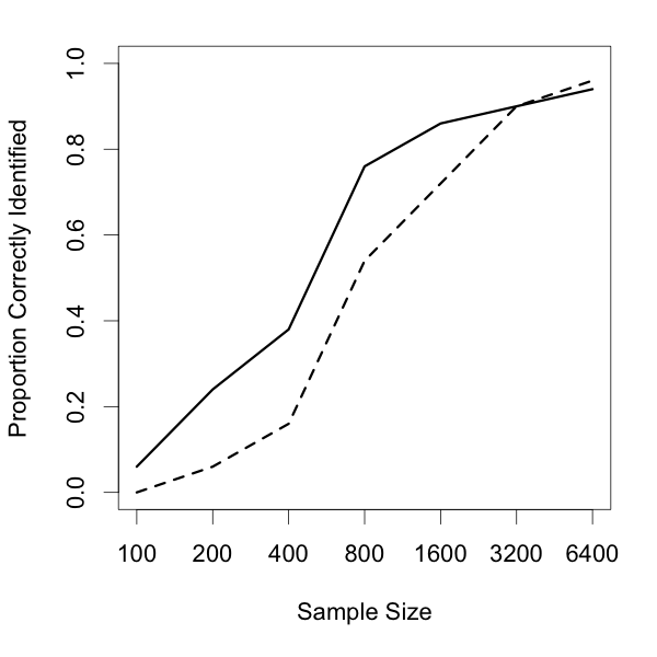
(a) $m=10$ leaves

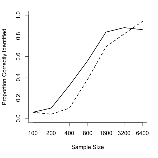
(b) $m=11$ leaves

Figure 6: Proportion of times, out of 50 simulations, sBIC (solid line) and BIC (dashed line) select the smallest true model for different samples sizes (displayed on a logarithmic scale).

Remark 5.1.

In the simulations, we evaluated the quality of the forests found by BIC and sBIC through the proportion of times the chosen forest matched the truth exactly. An exact match is a very strong requirement and one may instead wish to compute the average distance, based on some metric, between selected forest and the truth. Unfortunately, the most natural metrics in our setting are NP-hard to compute and can only be approximated in general [HJWZ96, HDRCB08].

5.2 Temperature Data

We consider a dataset consisting of average daily temperature values on 310 days from 37 cities across North America, South America, Africa, and Europe. The data was sourced from the National Climatic Data Center and compiled in a readily available format by the average daily temperature archive of the University of Dayton [oD]. In order to decorrelate and localize the data we first perform a seasonality adjustment where we regress each observed time series of temperature values on a sinusoid corresponding to the seasons and retain only the residuals. We then consider only the differences of average temperatures on consecutive days reducing the number of data points to $n=309$.

In the simulations of Section 5.1 we performed an exhaustive search over the lattice of all considered forests, a strategy which quickly becomes infeasible when increasing the number of observed variables beyond the low teens. Thus, in order to do model selection with the 37 observed nodes described above, we need to formulate an approximate sBIC. There are a plurality of possible heuristic strategies for producing this approximation involving combinations of greedy search, truncation of the considered model space, and simulated annealing. An in-depth exploration of these strategies and their relative performance is beyond the scope of this paper, instead we will show the results of using one such method as a proof of concept.

Our selection strategy, which we call a pruned chain search, has the following form:

• Generate an approximate maximum likelihood trivalent tree structure $T$.

• Prune the model space of considered forests to only consider a single decreasing path in the poset $\mathcal{P}_{T}$ starting at $T$ and ending with the empty forest.

• Compute the sBIC (or BIC) for models in the pruned space and select the highest scoring model.

Note that after (2) the number of considered models will equal to the number of observed variables making computation tractable for many observed nodes. We accomplish (1) using a version of the structural EM algorithm proposed by [FNPP02]. To produce the decreasing path of models in (2) we start with $T$ and iteratively select subforests in a greedy fashion:

• Suppose that after the $m$th iteration we have constructed the decreasing chain $\mathcal{C}_{m}$ of forests $T=F_{0}\supset F_{1}\supset F_{2}\supset...\supset F_{m}$.

• If $F_{m}$ is the empty forest then we are done.

• Otherwise, we extend $\mathcal{C}_{m}$ to $\mathcal{C}_{m+1}$ by adding to it the forest with largest BIC-penalized log-likelihood (with log-likelihood maximized using the EM algorithm described in Section 5.1) among all maximal subforests of $F_{m}$.

We present the results of applying above selection procedure to the temperature data in Figure 7. Note that the models selected by the sBIC and BIC are quite similar with the majority of the connections following our physical intuition that geographically adjacent cities should have similar temperature fluctuations while further separated cities should be essentially uncorrelated. For instance, all three cities in Washington, USA are connected to each other but to no other cities. The one difference between the the model selected by sBIC and that selected by the BIC is the connection of Barbados to the component containing the Bahamas in the sBIC graph. The distance between these nodes is just far enough to place this connection on the border between spurious and reasonable. As in the simulation experiments, we observe sBIC’s ability to select larger models.

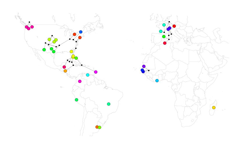
(a) Model chosen by sBIC

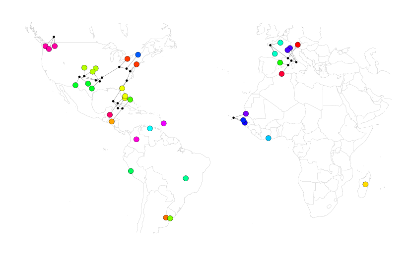
(b) Model chosen by BIC

Figure 7: The models selected by sBIC and BIC pruned chain search. Each colored node represents an observed node (nodes with the same color are from the same country or US state) and the black nodes correspond to latent variables. The position of colored nodes corresponds to the city from where the data was collected.

6 Conclusion

Real log-canonical thresholds and associated multiplicities quantify the large-sample properties of the marginal likelihood in Bayesian approaches to model selection. In this paper, we computed these RLCTs for Gaussian latent tree and forest models; the main results being Theorems 4.3 and 4.7. Our computations relied on the fact that the considered tree and forest models have a monomial parametrization, which allows one to apply methods from polyhedral geometry that we presented in Theorem 3.2.

Knowing RLCTs makes it possible to apply a ‘singular Bayesian information criterion’ (sBIC) that was recently proposed by [DP13]. RLCTs provide refined information about the marginal likelihood and our simulations show that, at least in smaller problems, the sBIC outperforms the usual BIC of [Sch78] that is defined using model dimension alone. As an exhaustive search over all models becomes quickly infeasible as the number of observed variables increases, we demonstrated, by example of a temperature dataset, how the sBIC might be approximated and applied to larger problems. In particular, we combined the structural EM of [FNPP02] with a greedy search methodology to reduce the number of considered models to a small collection for which the sBIC can be readily computed.

Appendix A Proof of Theorem 3.2

Let $H$ be the function from (3.1). By assumption, the ‘prior’ $\varphi:\Omega\to(0,\infty)$ is bounded above and $\mathcal{V}_{\Omega}(H)=\{\omega\in\Omega:H(\omega)=0\}$ is compact. Since $\varphi$ is smooth and positive, $\varphi$ is bounded away from zero on $\mathcal{V}_{\Omega}(H)$ and any compact neighborhood of this zero set. The poles of the zeta function in (2.6) can be shown to be the same for all such choices of $\varphi$, and we have ${\rm RLCT}_{\Omega}(H;\varphi)={\rm RLCT}_{\Omega}(H)$.

Our proof of Theorem 3.2 now proceeds in three steps:

• Show that ${\rm RLCT}_{\Omega}(H)={\rm RLCT}_{\Omega}(H^{0}+H^{1})$, where $H^{0}$, $H^{1}$ are the zero and nonzero parts of $H$ that are defined in (3.2) and (3.3).

• Show that ${\rm RLCT}_{\Omega_{1}}(H^{1})=(\lambda_{1},1)$, where $\lambda_{1}=\operatorname{codim}\mathcal{V}_{\Omega_{1}}(H^{1})$.

• Show that ${\rm RLCT}_{\Omega_{0}}(H^{0})=(\lambda_{0},\mathfrak{m})$, where $\lambda_{0}$ is the $\mathbf{1}$-distance of the Newton polyhedron $\Gamma_{+}(H^{0})$ and $\mathfrak{m}$ is the multiplicity (recall Definition 3.1).

Since $H^{0}$ and $H^{1}$ are functions of disjoint sets of coordinates and $\Omega=\Omega_{0}\times\Omega_{1}$ is a Cartesian product, it follows from Remark 7.2(3) in [Wat09] and the above Steps 1-3 that

$${\rm RLCT}_{\Omega}(H^{0}+H^{1})\;=\;(\lambda_{0}+\lambda_{1},(\mathfrak{m}+1)-1)\;=\;(\lambda_{0}+\lambda_{1},\mathfrak{m}),$$

which is the claim of Theorem 3.2.

Before moving on to Step 1 we make a definition. Let $f,g:\,\Omega\to[0,\infty)$ be two nonnegative functions with common zero set $\mathcal{V}_{\Omega}(g)=\mathcal{V}_{\Omega}(f)$. Then $f$ and $g$ are asymptotically equivalent, we write $f\sim g$, if there exist two constants $c,C>0$ and a neighborhood $W$ of $\mathcal{V}_{\Omega}(g)=\mathcal{V}_{\Omega}(f)$ such that

$$cf(\omega)\;\leq\;g(\omega)\;\leq\;Cf(\omega)$$ (A.1)

for all $\omega\in W\cap\Omega$. Note that $\sim$ is indeed an equivalence relation. According to Remark 7.2(1) in [Wat09], $f\sim g$ implies ${\rm RLCT}_{\Omega}(f)={\rm RLCT}_{\Omega}(g)$.

A.1 Step 1

First, note that ${\rm RLCT}_{\Omega}(H)={\rm RLCT}_{W\cap\Omega}(H)$ for any neighborhood $W$ of the compact zero set $\mathcal{V}_{\Omega}(H)$. Choose $W$ sufficiently small such that $\omega_{1},\ldots,\omega_{s}$ are bounded away from zero on $W\cap\Omega$. Next, by definition of the index $r$ in Section 3, we have that $H=H^{1}+H^{01}$, where

$$H^{01}=\sum_{i=r+1}^{k}\omega^{2u_{i}}.$$

When viewed as functions restricted to $W\cap\Omega$, we have $H^{0}\sim H^{01}$ because

$$\bigg{(}\min_{i}\prod_{j=1}^{s}\omega_{j}^{2u_{ij}}\bigg{)}\,H^{0}\;\leq\;H^{01}\;\leq\;\bigg{(}\max_{i}\prod_{j=1}^{s}\omega_{j}^{2u_{ij}}\bigg{)}\,H^{0}$$

and $\omega_{1},\ldots,\omega_{s}$ are bounded above and bounded away from zero on the compactum $W\cap\Omega$. It follows that ${\rm RLCT}_{\Omega}(H)={\rm RLCT}_{\Omega}(H^{0}+H^{1})$ because $H^{01}\sim H^{0}$ implies that $H^{1}+H^{0}\sim H^{1}+H^{01}=H$.

A.2 Step 2

To complete Step 2 we will prove the following result.

Proposition A.1.

Suppose that $H$ satisfies (3.1) with all $c_{i}^{*}\neq 0$, i.e., $H$ is equal to its nonzero part. Let $\mathcal{V}_{\Omega}(H)$ be the zero set of $H$ on $\Omega$. Then

$${\rm RLCT}_{\Omega}(H)=(\operatorname{codim}\mathcal{V}_{\Omega}(H),1).$$

Before turning to the proof, we exemplify the application of Proposition A.1.

Example A.2.

Let $\Omega=[0,1]\times[0,1]$ be the unit square in $\mathbb{R}^{2}$, and consider two functions $g_{1}(\omega)=(\omega_{1}-\omega_{2})^{2}$ and $g_{2}(\omega)=(\omega_{1}+\omega_{2})^{2}$. The zero set of either function is a line in $\mathbb{R}^{2}$. When restricting to $\Omega$, the zero set $\mathcal{V}_{\Omega}(g_{1})$ is a line segment and of codimension one. The zero set $\mathcal{V}_{\Omega}(g_{2})$, on the other hand, consists only of the origin and is of codimension two. We have ${\rm RLCT}_{\Omega}(g_{1})=(1,1)$ but ${\rm RLCT}_{\Omega}(g_{2})=(2,1)$.

To prove Proposition A.1, note first that when $H$ is equal to its nonzero part and $\mathcal{V}_{\Omega}(H)$ is compact, ${\rm RLCT}_{\Omega}(H)$ is equal to the RLCT of $H$ over a compact set on which all coordinates of the argument $\omega$ are bounded away from zero. Partition this compactum into the intersections with each one of the $2^{d}$ orthants in $\mathbb{R}^{d}$. Then ${\rm RLCT}_{\Omega}(H)$ is the minimum RLCT in any orthant. Similarly, the codimension of $\mathcal{V}_{\Omega}(H)$ is the minimum of any codimension obtained from intersection with an orthant. We may thus consider one orthant at a time. Changing signs as needed to make all coordinates positive, the following lemma becomes applicable.

Lemma A.3.

Let $W=[a_{1},b_{1}]\times\cdots\times[a_{s},b_{s}]$ with $0<a_{i}<b_{i}<\infty$. Let $\log W=[\log a_{1},\log b_{1}]\times\cdots\times[\log a_{s},\log b_{s}]$. If $H$ satisfies (3.1) with all $c_{i}^{*}>0$ and $\mathcal{V}_{W}(H)$ is nonempty, then

$${\rm RLCT}_{W}(H)={\rm RLCT}_{\log W}\left(\sum_{i=1}^{r}\left(u_{i}^{T}\omega-\log c_{i}^{*}\right)^{2}\right).$$

The result follows from a change of coordinates and an argument about asymptotic equivalence that has been used in other contexts. We include the proof of the lemma for sake of completeness.

Proof.

Change coordinates via the substitution $\tilde{\omega}=\log(\omega)$, where the logarithm is applied entry-wise. Since the Jacobian of this transformation is bounded above and bounded away from zero on $W$, it may be ignored in the computation of the RLCT and thus

$${\rm RLCT}_{W}(H)={\rm RLCT}_{\log W}\left(\sum_{i=1}^{r}\left(e^{u_{i}^{T}\omega}-e^{\log c_{i}^{*}}\right)^{2}\right).$$

Since $W$, and thus also $\log W$, is compact, each of the $r$ linear combinations $u_{i}^{T}\omega$ takes its values in a compact set. Restricted to this compact set, the function

$$h_{1}(x)\;=\;\sum_{i=1}^{r}\left(e^{x_{i}}-e^{\log c_{i}^{*}}\right)^{2}$$

is asymptotically equivalent to the sum of squares

$$h_{2}(x)\;=\;\sum_{i=1}^{r}\left(x_{i}-\log c_{i}^{*}\right)^{2},$$

as can been seen by a quadratic Taylor approximation to $h_{1}$ around the point $(\log c_{1}^{*},\dots,\log c_{r}^{*})$. Since asymptotically equivalent functions have the same RLCT, the claim is proven. ∎

By an application of Lemma A.3, the proof of Proposition A.1 reduces to an analysis of sums of squares of linear forms, that is, functions of the form

$$g(\omega)\;=\;\sum_{i=1}^{r}(u_{i}^{T}\omega-C^{*}_{i})^{2}$$ (A.2)

with $C_{i}^{*}\in\mathbb{R}$ and $u_{i}\in\mathbb{R}^{d}$. Proposition A.1 thus follows from Proposition A.4 below. Note that $\mathcal{V}_{\Omega}(g)$ is a polyhedron, which we assume to be nonempty.

Proposition A.4.

If $g:\Omega\to[0,\infty)$ is a sum of squares of linear forms as in (A.2) and $\Omega$ is a product of intervals, then ${\rm RLCT}_{\Omega}(g)=(\operatorname{codim}\mathcal{V}_{\Omega}(g),1)$.

Proof.

By [Lin11, Prop. 2.5, Prop. 3.2], or also [Wat09, Remark 2.14], ${\rm RLCT}_{\Omega}(g)$ is the minimum of local thresholds ${\rm RLCT}_{\Omega(x)}(g)$ over $x\in\mathcal{V}_{\Omega}(g)$. Here, each set $\Omega(x)=W(x)\cap\Omega$, where $W(x)$ is a sufficiently small neighbhorhood of $x$. We will show that ${\rm RLCT}_{\Omega(x)}(g)=(\operatorname{codim}\mathcal{V}_{\Omega}(g),1)$ for $x\in\mathcal{V}_{\Omega}(g)$, which implies our claim.

Consider any point $x\in\mathcal{V}_{\Omega}(g)$. By translation, we may assume without loss of generality that $x=0$ and $g(\omega)=\sum_{i}(u_{i}^{T}\omega)^{2}$. We may then take the neighborhood $\Omega(0)$ to be equal to $\{\omega\in\Omega:\max_{i}|\omega_{i}|\leq\varepsilon\}$ for sufficiently small $\varepsilon>0$.

When partitioning $\Omega(0)$ into orthants, the codimension of $\mathcal{V}_{\Omega}(g)$ is the minimum of the codimensions of the intersection between $\mathcal{V}_{\Omega}(g)$ and each one of the orthants. Furthermore, ${\rm RLCT}_{\Omega(0)}(g)$ is equal to the smallest RLCT of $g$ over any of these orthants. Therefore, changing the signs of the coordinates $\omega_{i}$ as needed, we are left with checking that ${\rm RLCT}_{\Omega_{+}}(g)$ is given by the codimension of $\mathcal{V}_{\Omega_{+}}(g)$ for $\Omega_{+}=\{\omega\in\Omega:0\leq\omega_{i}\leq\varepsilon\text{ for all }i=1,\dots,d\}$ and $g(\omega)=\sum_{i}(u_{i}^{T}\omega)^{2}$.

Case 1. If $\mathcal{V}_{{\Omega_{+}}}(g)$ intersects the interior of $\Omega_{+}$, then we may pick any point $x_{+}$ in this intersection and consider $\Omega_{+}$ as a neighborhood of $x_{+}$. After a change of coordinates, we have $g(\omega)=\omega_{1}^{2}+\dots+\omega_{s}^{2}$, where $s$ is the codimension of $\mathcal{V}_{\Omega_{+}}(g)$. By Example 3.4, ${\rm RLCT}_{\Omega_{+}}(g)=(s,1)$, which was to be shown.

Case 2. Suppose now that $\mathcal{V}_{{\Omega_{+}}}(g)$ is contained in the boundary of ${\Omega_{+}}$. Since the zero set of $g$ on all of $\mathbb{R}^{d}$ is a linear space, $\mathcal{V}_{{\Omega_{+}}}(g)$ is in fact a face of ${{\Omega_{+}}}$, and each $u_{i}^{T}\omega$ is a supporting hyperplane of $\Omega_{+}$. In particular, after appropriate sign changes, we may assume that $u_{i}^{T}\omega\geq 0$ on $\Omega_{+}$. The codimension of $\mathcal{V}_{{\Omega_{+}}}(g)$ is equal to the number, say $s$, of facets of $\Omega_{+}$ containing it. Without loss of generality, we may assume that these facets are given by $\omega_{1}=0$, $\omega_{2}=0$, …, $\omega_{s}=0$. This implies that all $u_{i}$ have nonzero entries only in the first $s$ coordinates. We now show that when restricted to $\Omega_{+}$, the functions $g(\omega)$ and $f(\omega)=\omega_{1}^{2}+\dots+\omega_{s}^{2}$ are asymptotically equivalent; recall (A.1).

To show that on $\Omega_{+}$, the function $g$ can be bounded from below by a positive multiple of $f$, note that the fact that $u_{i}^{T}\omega\geq 0$ on $\Omega_{+}$ implies that all $u_{i}$ have nonnegative entries. Hence,

$$\sum_{i=1}^{r}(u_{i}^{T}\omega)^{2}\;=\;\sum_{i=1}^{r}\Bigg{(}\sum_{j=1}^{s}u_{ij}\omega_{j}\Bigg{)}^{2}\;\geq\;\sum_{j=1}^{s}\left(\sum_{i=1}^{r}u_{ij}^{2}\right)\omega_{j}^{2},$$

where the inequality is obtained by expanding squares and dropping the mixed terms, which are nonnegative. If $\sum_{i=1}^{r}u_{ij}^{2}=0$ for some index $j$ then $u_{ij}=0$ for all $i$, which contradicts the fact that $\omega_{j}=0$ for all $\omega\in\mathcal{V}_{\Omega_{+}}(g)$. Thus,

$$c\;=\;\min\left\{\sum_{i=1}^{r}u_{ij}^{2}:1\leq j\leq s\right\}\;>\;0,$$

and $g(\omega)\geq cf(\omega)$ for all $\omega\in\Omega_{+}$.

To prove that $g$ can be bounded above by a multiple of $f$, note that all $u_{i}^{T}\omega$ are nonnegative on $\Omega_{+}$ and thus

$$\sum_{i=1}^{r}(u_{i}^{T}\omega)^{2}\;\leq\;\left(\sum_{i=1}^{r}u_{i}^{T}\omega\right)^{2}\;=\;\Bigg{(}\sum_{i=1}^{r}\sum_{j=1}^{s}u_{ij}\omega_{j}\Bigg{)}^{2}.$$

Let $u_{+j}=\sum_{i}u_{ij}$ and $u_{++}=\sum_{j}u_{+j}$. Then, since all $u_{i}$ have nonnegative entries, Jensen’s inequality implies that

$$\Bigg{(}\sum_{i=1}^{r}\sum_{j=1}^{s}u_{ij}\omega_{j}\Bigg{)}^{2}\;=\;u_{++}^{2}\Bigg{(}\sum_{j=1}^{s}\frac{u_{+j}}{u_{++}}\omega_{j}\Bigg{)}^{2}\;\leq\;u_{++}\,\max\{u_{+j}:1\leq j\leq s\}\sum_{i=1}^{s}\omega_{i}^{2}.$$

Since $g$ is asymptotically equivalent to $f(\omega)=\omega_{1}^{2}+\dots+\omega_{s}^{2}$, we have ${\rm RLCT}_{\Omega_{+}}(g)={\rm RLCT}_{\Omega_{+}}(f)$. Let $\Omega_{+}^{\prime}=[-\epsilon,\epsilon]^{s}\times[0,\epsilon]^{d-s}$. Then

$$\int_{\Omega_{+}}(\omega_{1}^{2}+\ldots+\omega_{s}^{2})^{-z/2}\,d\omega\;=\;2^{-s}\int_{\Omega_{+}^{\prime}}(\omega_{1}^{2}+\ldots+\omega_{s}^{2})^{-z/2}\,d\omega.$$

Hence, ${\rm RLCT}_{\Omega_{+}}(f)={\rm RLCT}_{\Omega_{+}^{\prime}}(f)$. From Case 1, we know that ${\rm RLCT}_{\Omega_{+}^{\prime}}(f)\;=\;(s,1)$. Putting it all together, we have shown that ${\rm RLCT}_{\Omega_{+}}(g)=(s,1)$. ∎

A.3 Step 3

The remaining step amounts to proving the following result, which concerns the case where the considered function $H$ is equal to its zero part.

Proposition A.5.

Let $\Omega$ be a compact product of intervals containing the origin, and let $\Gamma_{+}(H)$ be the Newton polyhedron of the function $H(\omega)=\sum_{i}\omega^{2u_{i}}$. Then

$${\rm RLCT}_{\Omega}(H)=(\lambda,\mathfrak{m}),$$

where $1/\lambda$ is the $\mathbf{1}$-distance of $\Gamma_{+}(H)$ and $\mathfrak{m}$ is its multiplicity.

Proof.

Note that $H$ is invariant under sign changes. Hence, ${\rm RLCT}_{\Omega}(H)={\rm RLCT}_{\Omega^{\prime}}(H)={\rm RLCT}_{\Omega\cup\Omega^{\prime}}(H)$ when $\Omega^{\prime}$ is obtained from $\Omega$ by changing the signs of any subset of the coordinates $\omega_{1},\dots,\omega_{d}$. Forming the unions of $\Omega$ and its reflected versions shows that in order to prove Proposition A.5, we may assume that the origin is an interior point of $\Omega$. The claim now follows from Theorem 8.6 in [AGZV88], see also [Lin11, Section 4], and by Remark A.6 below. ∎

Remark A.6.

When the origin is in the interior of $\Omega$, the function $H(\omega)=\sum_{i}\omega^{2u_{i}}$ has ${\rm RLCT}_{\Omega}(H)={\rm RLCT}_{\Omega(0)}(H)$ for any small neighborhood $\Omega(0)$ of the origin. Indeed, as mentioned in the proof of Proposition A.4, ${\rm RLCT}_{\Omega}(H)$ is the minimum of local RLCTs of $H$ in small neighborhoods $\Omega(x)$ of points $x\in\Omega$. If $x\not=0$, then some of the variables, say $\omega_{1},\ldots,\omega_{s}$, are bounded away from zero on a sufficiently small neighborhood $\Omega(x)$. Substituting these variables by $\omega_{1}-x_{1},\ldots,\omega_{s}-x_{s}$, respectively, in $H$, we get a new function $H_{x}$ for which ${\rm RLCT}_{\Omega(0)}(H)={\rm RLCT}_{\Omega(x)}(H_{x})$. Now, $0\leq H_{x}\leq H$ near $x$. Consequently, ${\rm RLCT}_{\Omega(x)}(H_{x})\leq{\rm RLCT}_{\Omega(x)}(H)$. We conclude that ${\rm RLCT}_{\Omega(0)}(H)\leq{\rm RLCT}_{\Omega(x)}(H)$.

Appendix B Proof of Theorem 4.3

Let $T=(U,E)$ be a tree with set of leaves $V$, and let $q$ be a distribution in the latent tree model $\mathbf{M}(T)$, which has parameter space $\Omega=(0,\infty)^{V}\times[-1,1]^{E}$. We are to compute ${\rm RLCT}_{\Omega}(H_{q})$ for the function $H_{q}$ from (4.1), where $\omega_{v}^{*}$ and $\rho_{vw}^{*}$ are the variances and correlations of the distribution $q$. The basic idea of this proof follows [Zwi11].

First, observe that Theorem 3.2 is applicable to this problem. Indeed, $H_{q}$ has the form from (3.1) and the $q$-fiber $\mathcal{V}_{\Omega}(H_{q})$ is compact. Compactness holds because $H_{q}(\omega)=0$ implies that $\omega_{v}=\omega_{v}^{*}$ for all $v\in V$, and all edge correlations $\omega_{e}$, $e\in E$, are in the compact interval $[-1,1]$.

Now, let $F^{*}:=F^{*}(q)=(U^{*},E^{*})$ be the $q$-forest, and let $H_{q}^{1}(\omega_{1},\ldots,\omega_{s})$ be the nonzero part of $H_{q}$ given in (4.2). The set $\mathcal{V}_{\Omega_{1}}(H_{q}^{1})$ is equal to the $q$-fiber under the model $\mathbf{M}(F^{*})$; recall that $\Omega_{1}$ is the projection of $\Omega$ onto the first $s$ coordinates. We deduce that $\operatorname{codim}\mathcal{V}_{\Omega_{1}}(H_{q}^{1})=\dim\mathbf{M}(F^{*})$, which gives the value of $\lambda_{1}$ in Theorem 3.2. It remains to show that the zero part $H_{q}^{0}(\omega_{s+1},\ldots,\omega_{d})$ defined in (4.3) satisfies

$$(\lambda_{0},\mathfrak{m})\;=\;{\rm RLCT}_{\Omega_{0}}(H_{q}^{0})\;=\;\left(\frac{1}{2}\sum_{e\in E_{0}}w(e),1+l_{2}^{\prime}\right),$$ (B.1)

where $\Omega_{0}$ is the projection of $\Omega$ onto the last $d-s$ coordinates, $E_{0}=E\setminus E^{*}$ is the set of edges that appear in $T$ but not in $F^{*}$, and $l_{2}^{\prime}$ is the number of degree two nodes of $T$ that are not in $U^{*}$.

The zero part of $H_{q}$ is the sum of squares of the monomials

$$\prod_{e\in\overline{vw}\cap E_{0}}\omega_{e},\qquad v,w\in V,\;v\not\sim w;$$ (B.2)

recall that $v\not\sim w$ if there is no path between $v$ and $w$ in the $q$-forest $F^{*}=(U^{*},E^{*})$. The edge set $E_{0}$ can be partitioned into sets $E_{01},\dots,E_{0t}$ such that each $E_{0i}$ defines a tree $S_{i}=(U_{i},E_{0i})$ that has the set of nodes $L_{i}:=U_{i}\cap U^{*}$ as leaves. In other words, the set of leaves $L_{i}$ of tree $S_{i}$ comprises precisely those nodes that belong to both $S_{i}$ and the $q$-forest $F^{*}$. For example, in Figure 1, we have $t=1$ and $S_{1}$ is the tree with one inner node $b$ and three leaves $a,3,4$. As a further example, consider the tree and $q$-forest in Figure 8(a) and (b), for which we form two subtrees $S_{1}$ and $S_{2}$ with edge sets $E_{01}=\{\{a,3\}\}$ and $E_{02}=\{\{a,4\}\}$, as shown in Figure 8(c) and (d). In this second example, the sets of leaves are $L_{1}=\{a,3\}$ and $L_{2}=\{a,4\}$, illustrating that the sets $L_{1},\dots,L_{t}$ need not be disjoint.

(a)    (b)    (c)    (d)

Figure 8: (a) Star tree; (b) $q$-forest when $\rho_{12}^{*}$ is the only nonzero correlation; (c),(d) subtrees formed from the removed edges.

Consider now the function $\tilde{H}_{q}^{0}$ given by the sum of squares of the monomials

$$\prod_{e\in\overline{uu^{\prime}}}\omega_{e},\qquad i\in[t],\;u,u^{\prime}\in L_{i},\,u\not=u^{\prime},$$ (B.3)

where $[t]=\{1,\dots,t\}$ and $\overline{uu^{\prime}}$ refers to the unique path between $u$ and $u^{\prime}$ in tree $S_{i}$. Each monomial listed in (B.3) is also listed in (B.2). To see this, observe that two distinct nodes $u,u^{\prime}\in L_{i}$ belong to distinct connected components in $F^{*}$. If we take $v\in V$ from one of the two connected components and $w\in V$ from the other, then the monomial they define in (B.2) is equal to the monomial that $u$ and $u^{\prime}$ define in (B.3). Moreover, by the definition of the trees $S_{i}$, every monomial listed in (B.2) is the product of monomials from (B.3). It follows that the Newton polyhedra $\Gamma_{+}(H_{q}^{0})$ and $\Gamma_{+}(\tilde{H}_{q}^{0})$ are equal and hence ${\rm RLCT}_{\Omega_{0}}(H_{q}^{0})={\rm RLCT}_{\Omega_{0}}(\tilde{H}_{q}^{0})$ (c.f. Proposition A.5).

Let $f_{i}$ be the sum of squares of the monomials in (B.3) that are associated with pairs of distinct nodes $u$ and $u^{\prime}$ in the set of leaves $L_{i}$ of the tree $S_{i}$. No two trees $S_{i}$ and $S_{j}$ for $i\not=j$ share an edge. Hence, the two sums of squares $f_{i}$ and $f_{j}$ depend on different subvectors of $\omega$. Since $\tilde{H}_{q}^{0}=f_{1}+\cdots+f_{t}$, it follows from (2.5) that

$${\rm RLCT}_{\Omega_{0}}(H_{q}^{0})=\sum_{i=1}^{t}{\rm RLCT}_{\Omega_{0}}(f_{i})-(0,t-1);$$ (B.4)

see also Remark 7.2(3) in [Wat09]. If $T$ has no nodes of degree two, i.e., $l_{2}=l_{2}^{\prime}=0$, then the same is true for the each tree $S_{i}$. Lemma B.1 below then implies that

$${\rm RLCT}_{\Omega_{0}}(f_{i})=\left(\frac{|L_{i}|}{2},1\right).$$ (B.5)

Since the nodes in $L_{i}$ lie in $F^{*}$, we have

$$\sum_{i=1}^{t}|L_{i}|=\sum_{e\in E_{0}}w(e),$$ (B.6)

where $w(e)\in\{0,1,2\}$ is the number of nodes of $e$ that lie in the $q$-forest $F^{*}$. Combining (B.4)-(B.6), we obtain (B.1) and have thus proven Theorem 4.3 in the case of $l_{2}=0$ nodes of degree two. The case with nodes of degree two follows the same way applying Lemma B.2 instead of Lemma B.1.

Lemma B.1.

Let $S=(V,E)$ be a tree with set of leaves $L$ and all inner nodes of degree at least three. Let $f$ be the sum of squares of the monomials

$$\prod_{e\in\overline{vw}}\omega_{e},\qquad v,w\in L,\;v\not=w.$$ (B.7)

If $\Omega$ is a neighborhood of the origin, then

$${\rm RLCT}_{\Omega}(f)=\left(\frac{|L|}{2},1\right).$$

Proof.

If $|L|=2$, then $S$ has a single edge and no inner nodes. In this case, $f$ is the square of a single variable and it is clear ${\rm RLCT}_{\Omega}(f)=(1,1)=(|L|/2,1)$. In the remainder of this proof, we assume that $|L|\geq 3$.

By Proposition A.5, it suffices to compute the $\mathbf{1}$-distance and its multiplicity for the Newton polyhedron $\Gamma_{+}(f)\subset\mathbb{R}^{E}$. By Definition 3.1, the polyhedron $\Gamma_{+}(f)$ is determined by the exponent vectors of the monomials in (B.7). Each exponent vector is the incidence vector for a path between a pair of leaves. In other words, each pair of two distinct leaves $v$ and $w$ defines a vector $u\in\mathbb{R}^{E}$ with $u_{e}=1$ if $e\in\overline{vw}$ and $u_{e}=0$ otherwise. Write $\mathcal{U}$ for the set of all these $\binom{|L|}{2}$ vectors.

Let $E_{L}$ be the set of terminal edges of $S$, i.e., the $|L|$ edges that are incident to a leaf. We claim that every point $x$ in the Newton polyhedron $\Gamma_{+}(f)$ satisfies

$$\sum_{e\in E_{L}}x_{e}\geq 2$$ (B.8)

and that the inequality defines a facet of $\Gamma_{+}(f)$. Indeed, if $x\in\mathcal{U}$ then $\sum_{e\in E_{L}}x_{e}=2$ because every path between two leaves in $L$ includes precisely two edges in $E_{L}$. It is then clear that (B.8) holds for all points $x\in\Gamma_{+}(f)$. Moreover, by [MP08, Lemma 1], the span of $\mathcal{U}$ is all of $\mathbb{R}^{E}$. Hence, the affine hull of $\mathcal{U}$ is the hyperplane given by $\sum_{e\in E_{L}}x_{e}=2$, and we conclude that (B.8) defines a facet of $\Gamma_{+}(f)$.

Since $|E_{L}|=|L|$, inequality (B.8) implies that the $\mathbf{1}$-distance of $\Gamma_{+}(f)$ is at least $2/|L|$. We claim that it is equal to $2/|L|$. In fact, we will show that the vector $\frac{2}{|L|}\mathbf{1}$ not only lies in the Newton polyhedron but also in the Newton polytope $\Gamma(f)$, that is, the vector is a convex combination of the incidence vectors in $\mathcal{U}$. To prove this, we construct a set of paths $\mathcal{P}$ in the tree $S$ such that (i) each element of $\mathcal{P}$ is a path between leaves of $S$, (ii) $\mathcal{P}$ contains precisely $|L|$ paths, and (iii) every edge of $S$ is covered by exactly two paths of $\mathcal{P}$. The construction implies our claim because the average of the incidence vectors of the paths in $\mathcal{P}$ is equal to $\frac{2}{|L|}\mathbf{1}$.

Let $S^{*}$ be any trivalent tree that has the same set of leaves $L$ as $S$ and that can be obtained from $S^{*}$ by edge contraction. Here, a tree is trivalent if each inner node has degree three. We will use induction on the number of leaves to show that a set of paths $\mathcal{P}$ with the desired properties (i)-(iii) exists. Figure 9 shows an example.

If $S^{*}$ has three $|L|=3$ leaves, then there is a single inner node and each path between two leaves has two edges. We may simply take $\mathcal{P}$ to be the set of all the three paths that exist between pairs of leaves. This provides the induction base.

In the induction step, pick two leaves $v$ and $w$ of the tree $S^{*}$ that are joined by a path with two edges $\{v,a\}$ and $\{a,w\}$. The node $a$ is an inner node of $S^{*}$. Remove the two edges and the two leaves to form a subtree $S^{**}$, in which $a$ becomes a leaf. Then $S^{**}$ has $|L|-1$ leaves and, by the induction hypothesis, there is a set of paths $\mathcal{P}^{**}$ that satisfies properties (i)-(iii) with respect to $S^{**}$. In particular, $|\mathcal{P}^{**}|=|L|-1$. Now, precisely two paths in $\mathcal{P}^{**}$ have the node $a$ as an endpoint. Extend one of them by adding the edge $\{a,v\}$ and extend the other by adding $\{a,w\}$. This gives two paths between leaves of $S^{*}$. All other paths in $\mathcal{P}^{**}$ are already paths between leaves of $S^{*}$. Add one further path, namely, $(v,a,w)$, and denote the resulting collection of $|L|$ paths by $\mathcal{P}^{*}$. Clearly, the set $\mathcal{P}^{*}$ satisfies properties (i)-(iii) with respect to $S^{*}$. Contracting each path in $\mathcal{P}^{*}$ by applying the edge contractions that transform $S^{*}$ into $S$, we obtain a system of paths $\mathcal{P}$ that satisfies properties (i)-(iii) with respect to $S$.

Figure 9: An example of a system of paths such that each edge of a trivalent tree is covered by exactly two paths.

Finally, note that in the construction we just gave we can ensure that $\mathcal{P}$ includes a given path between two leaves in $L$. Hence, the vector $\frac{2}{|L|}\mathbf{1}$ can be written as a convex combination of vertices of $\Gamma(f)$ such that a given vertex $x$ get positive weight. It follows that $\frac{2}{|L|}\mathbf{1}$ lies in the interior of the Newton polytope and thus the multiplicity $\mathfrak{m}$ is $1$. ∎

The next result generalizes the previous lemma to the case of trees with nodes of degree 2. We remark Example 2.2 is a special case of this generalization. It matches the case where the tree $S$ has two leaves and one inner node, which is then necessarily of degree two.

Lemma B.2.

Let $S=(V,E)$ be a tree with set of leaves $L$, and let $f$ be the sum of squares of the monomials

$$\prod_{e\in\overline{vw}}\omega_{e},\qquad v,w\in L,\;v\not=w.$$ (B.9)

If $\Omega$ is a neighborhood of the origin, then

$${\rm RLCT}_{\Omega}(f)=\left(\frac{|L|}{2},1+l_{2}\right)$$

where $l_{2}$ is the number of (inner) nodes of $S$ that have degree two.

Proof.

Suppose $a$ is an inner node of degree two, and that $a$ is incident to the two edges $e=\{a,b\}$ and $f=\{a,c\}$. Then any path connecting to leaves in $L$ either uses both $e$ and $f$ or neither $e$ nor $f$. Hence, if $x$ is the incidence vector of a path between two leaves in $L$, then $x_{e}=x_{f}$. It follows that the affine hull of Newton polytope generated by the path incidence vectors is no longer a hyperplane but an affine space of dimension $|E|-1-l_{2}$.

Proceeding exactly as in the proof of Lemma B.1, we see that it still holds that the $\mathbf{1}$-distance of the Newton polyhedron $\Gamma_{+}(f)$ is $2/|L|$. Similarly, the ray spanned by $\mathbf{1}$ still meets $\Gamma_{+}(f)$ in the relative interior of the Newton polytope $\Gamma(f)$. However, since the codimension of the Newton polytope is now $1+l_{2}$, we have ${\rm RLCT}_{\Omega}(f)=(|L|/2,1+l_{2})$. ∎

References

- [AGZV88] Vladimir I. Arnold, Sabir M. Guseĭn-Zade, and Aleksandr N. Varchenko, Singularities of Differentiable Maps, vol. II, Birkhäuser, 1988.
- [CL68] C. K. Chow and C. N. Liu, Approximating discrete probability distributions with dependence trees, IEEE Trans. Inform. Theory 14 (1968), 462–467.
- [CTAW11] Myung Jin Choi, Vincent Y. F. Tan, Animashree Anandkumar, and Alan S. Willsky, Learning latent tree graphical models, J. Mach. Learn. Res. 12 (2011), 1771–1812.
- [DP13] Mathias Drton and Martyn Plummer, A Bayesian information criterion for singular models, arXiv:1309.0911, September 2013.
- [Drt09] Mathias Drton, Likelihood ratio tests and singularities, Ann. Statist. 37 (2009), no. 2, 979–1012.
- [DSS09] Mathias Drton, Bernd Sturmfels, and Seth Sullivant, Lectures on algebraic statistics, Oberwolfach Seminars, vol. 39, Birkhäuser Verlag, Basel, 2009.
- [EdAL10] David Edwards, Gabriel de Abreu, and Rodrigo Labouriau, Selecting high-dimensional mixed graphical models using minimal AIC or BIC forests, BMC Bioinformatics 11 (2010), no. 1, 18.
- [FNPP02] Nir Friedman, Matan Ninio, Itsik Pe’er, and Tal Pupko, A structural EM algorithm for phylogenetic inference, Journal of Computational Biology 9 (2002), no. 2, 331–353.
- [HDRCB08] Glenn Hickey, Frank Dehne, Andrew Rau-Chaplin, and Christian Blouin, Spr distance computation for unrooted trees, Evolutionary bioinformatics online 4 (2008), 17.
- [HJWZ96] Jotun Hein, Tao Jiang, Lusheng Wang, and Kaizhong Zhang, On the complexity of comparing evolutionary trees, Discrete Appl. Math. 71 (1996), no. 1-3, 153–169. MR 1420297 (98f:92004)
- [Lau96] Steffen L. Lauritzen, Graphical models, Oxford Statistical Science Series, vol. 17, Oxford University Press, 1996, Oxford Science Publications.
- [Lin11] Shaowei Lin, Asymptotic approximation of marginal likelihood integrals, arXiv:1003.5338, November 2011.
- [MP08] Radu Mihaescu and Lior Pachter, Combinatorics of least-squares trees, Proc. Natl. Acad. Sci. USA 105 (2008), no. 36, 13206–13211.
- [MRS13] Elchanan Mossel, Sébastien Roch, and Allan Sly, Robust estimation of latent tree graphical models: Inferring hidden states with inexact parameters, IEEE Trans. Inform. Theory 59 (2013), no. 7, 4357–4373.
- [oD] University of Dayton, Environmental protection agency average daily temperature archive, http://academic.udayton.edu/kissock/http/Weather/default.htm, Accessed: 2015-09-20.
- [RG05] Dmitry Rusakov and Dan Geiger, Asymptotic model selection for naive Bayesian networks, J. Mach. Learn. Res. 6 (2005), 1–35 (electronic).
- [Sch78] Gideon Schwarz, Estimating the dimension of a model, Ann. Statist. 6 (1978), no. 2, 461–464.
- [SGS00] Peter Spirtes, Clark Glymour, and Richard Scheines, Causation, prediction, and search, second ed., Adaptive Computation and Machine Learning, MIT Press, Cambridge, MA, 2000, With additional material by David Heckerman, Christopher Meek, Gregory F. Cooper and Thomas Richardson, A Bradford Book.
- [TAW11] Vincent Y. F. Tan, Animashree Anandkumar, and Alan S. Willsky, Learning high-dimensional Markov forest distributions: analysis of error rates, J. Mach. Learn. Res. 12 (2011), 1617–1653.
- [Wat09] Sumio Watanabe, Algebraic geometry and statistical learning theory, Cambridge Monographs on Applied and Computational Mathematics, vol. 25, Cambridge University Press, Cambridge, 2009.
- [Wat10a] , Asymptotic equivalence of Bayes cross validation and widely applicable information criterion in singular learning theory, J. Mach. Learn. Res. 11 (2010), 3571–3594.
- [Wat10b] Sumio Watanabe, Equations of states in singular statistical estimation, Neural Networks 23 (2010), no. 1, 20–34.
- [YW12] Koshi Yamada and Sumio Watanabe, Statistical learning theory of quasi-regular cases, IEICE Transactions on Fundamentals of Electronics, Communications and Computer Sciences 95 (2012), no. 12, 2479–2487.
- [Zwi11] Piotr Zwiernik, Asymptotic behaviour of the marginal likelihood for general Markov models, J. Mach. Learn. Res. 12 (2011), 3283–3310.