Randomized Algorithms for Large-scale Inverse Problems
with General Regularizations

Abstract

We shall investigate randomized algorithms for solving large-scale linear inverse problems with general regularizations. We first present some techniques to transform inverse problems of general form into the ones of standard form, then apply randomized algorithms to reduce large-scale systems of standard form to much smaller-scale systems and seek their regularized solutions in combination with some popular choice rules for regularization parameters. Then we will propose a second approach to solve large-scale ill-posed systems with general regularizations. This involves a new randomized generalized SVD algorithm that can essentially reduce the size of the original large-scale ill-posed systems. The reduced systems can provide approximate regularized solutions with about the same accuracy as the ones by the classical generalized SVD, and more importantly, the new approach gains obvious robustness, stability and computational time as it needs only to work on problems of much smaller size. Numerical results are given to demonstrated the efficiency of the algorithms.

Keywords. Generalized SVD, randomized algorithm, regularization, inverse problems

1 Introduction

Tikhonov regularization is one of the most popular and effective techniques for the ill-conditioned linear system $Ky=b$ arising from the discretization of some linear or nonlinear inverse problems [1, 3, 7], where $K$ is an $m\times n$ matrix and $b$ is an $m\times 1$ vector obtained from measurement data. The standard Tikhonov regularization of this problem is of the form

$$\min_{y}||Ky-b||^{2}+\mu^{2}||y||^{2},$$ (1)

where $\mu$ is the regularization parameter, and the 2-norm $\|\cdot\|$ is used in this work unless otherwise specified. We will call formulation (1) as the standard form, where the second term is for the regularization of the solution and the identity operator is used for the regularisation. The identity regularisation is the simplest and most convenient one, but it may not be the best in most applications. When we know some additional a priori information about the physical solution for a practical problem, we may apply some other more effective regularisations. To differentiate from the standard one (1), we will adopt other notation for the general linear ill-conditioned system, namely $Ax=b$, where $A$ is an $m\times n$ matrix and $b$ is an $m\times 1$ vector. Then the associated Tikhonov regularization in more general form is of the form

$$\min_{x}||Ax-b||^{2}+\mu^{2}||Lx||^{2},$$ (2)

where the matrix $L$ is a $p\times n$ matrix, which may be a discrete approximation to some differential operator, for example, the discrete Laplacian or gradient operator. When the null spaces of $A$ and $L$ intersect trivially, i.e., $\mathcal{N}(A)\cap\mathcal{N}(L)=\{0\}$, the regularised Tikhonov solution of (2) is unique. As we shall see, the general form (2) can be transformed into the standard one (1) for very general regularisation $L$.

When system (1) or (2) is large-scale, the traditional methods based on singular value decomposition (SVD) or generalized SVD are very expensive and unstable, and often infeasible for practical implementations. For large-scale discrete systems (1) of standard form, we can apply the randomized SVD (RSVD) [17] to essentially reduce the problem size, then combine the L-curve, GCV, and other discrepancy principles to locate reasonable regularization parameters for solving the reduced regularisation systems. In this work, we shall focus on the solution of the general form (2) of Tikhonov regularization. In section 2, we discuss several techniques to transform the general form into the standard one, then use the strategies in [17] to solve the standard system. In section 3, we consider the general form directly, and introduce a new randomized generalized SVD (RGSVD) to reduce the problem size and then seek the regularised solution. Numerical experiments are given in section 4.

2 Transformation into standard form and RSVD

In this section we first discuss a general strategy to transform the problem (2) of general form into the standard one (1), then apply the similar strategy as used in [17], which combines the randomized SVD with some choice rules on regularization parameters, to solve the standard system.

2.1 General transformation into the standard system

We demonstrate now how to transform the problem (2) of general form with different regularisation operators $L$ into the standard one (1). Usually we assume that $\mathcal{N}(A)\cap\mathcal{N}(L)=\{0\}$, such that the solution of (2) is unique. For the cases where the matrix $L$ is of full column rank, this assumption is automatically satisfied. But we shall consider the most general case without this assumption, including both cases: $\mathcal{N}(A)\cap\mathcal{N}(L)\neq\{0\}$ and $\mathcal{N}(A)\cap\mathcal{N}(L)=\{0\}$. For the case with $\mathcal{N}(A)\cap\mathcal{N}(L)\neq\{0\}$, the solution of (2) is not unique, so least-squares solutions with minimum norm will be sought. In the sequel, we shall often use the Moore-Penrose generalized inverse $L^{\dagger}$ of matrix $L$ [8].

We start with the following theorem which unifies the transformations of problem (2) into the standard one (1) for all possibilities, and will discuss in section 2.3 several cases when $A$ and $L$ have special structures, where the results can be simplified.

Theorem 1.

Let $W$, $Z$ and $P$ be any matrices satifying

$$\mathcal{R}(W)=\mathcal{N}(L),\quad\mathcal{R}(Z)=\mathcal{R}(L),\quad Z^{T}Z=I,\quad\mathcal{R}(P)=\mathcal{R}^{\perp}(AW),\quad P^{T}P=I,$$

and $L^{\#}=(I-W(AW)^{\dagger}A)L^{\dagger}$. Then the least-squares solution with minimum norm to the problem (2) of general form can be given by

$$x_{\mu}=L^{\#}Zy_{\mu}+W(AW)^{\dagger}b,$$ (3)

where $y_{\mu}$ is the minimizer of the following problem

$$\min_{y}||P^{T}AL^{\dagger}Zy-P^{T}b||^{2}+\mu^{2}||y||^{2}.$$ (4)

Equivalently, $y_{\mu}$ can be obtained by solving

$$\min_{y}\{||AL^{\#}Zy-b||^{2}+\mu^{2}||y||^{2}\}.$$ (5)

Proof. Consider the SVD of matrix $L$:

$$L=U\Sigma V^{T}=\begin{pmatrix}U_{1},U_{2}\end{pmatrix}\begin{bmatrix}\Sigma_{1}&\\ &0\end{bmatrix}\begin{pmatrix}V_{1}^{T}\\ V_{2}^{T}\end{pmatrix}=U_{1}\Sigma_{1}V_{1}^{T},$$ (6)

where $U=[U_{1},U_{2}]$ and $V=[V_{1},V_{2}]$ are unitary matrices, $\Sigma_{1}$ includes the nonzero singular values in the diagonal matrix $\Sigma$.

For any vector $x\in\mathbb{R}^{n}$, we write it as $x=V_{1}\Sigma_{1}^{-1}\widehat{y}+V_{2}\widehat{z}$, i.e., $x=L^{\dagger}U_{1}\widehat{y}+V_{2}\widehat{z}$. Since $span\{Z\}=\mathcal{R}(L)=span\{U_{1}\}$ and $span\{W\}=\mathcal{N}(L)=span\{V_{2}\}$, we can set

$$x=L^{\dagger}Zy+Wz.$$

Now we apply the complete orthogonal decomposition on the matrix $AW$ [8]:

$$Q^{T}(AW)\Pi=\begin{bmatrix}T_{11}&0\\ 0&0\end{bmatrix},$$

where $Q$ and $\Pi$ are orthogonal matrices, and $T_{11}$ is nonsingular matrix with the dimension determined by the rank of $AW$. For the case where $\mathcal{N}(A)\cap\mathcal{N}(L)=\{0\}$, the matrix $AW$ is of full column rank, and the zero matrix on the right side of $T_{11}$ will disappear. For the more general case with $\mathcal{N}(A)\cap\mathcal{N}(L)\neq\{0\}$, the matrix $AW$ is not of full column rank. Let $Q=[Q_{1},Q_{2}]$ be partitioned in compatible dimensions with $T_{11}$. Then we have $span\{Q_{1}\}=\mathcal{R}(AW)$, and $span\{Q_{2}\}=\mathcal{R}^{\perp}(AW)$ [8]. And it is easy to verify that

$$||Ax-b||^{2}+\mu^{2}||Lx||^{2}$$

$$= ||Q^{T}AL^{\dagger}Zy+Q^{T}AW\Pi(\Pi^{T}z)-Q^{T}b||^{2}+\mu^{2}||LL^{\dagger}Zy||^{2}$$

$$= ||Q_{1}^{T}AL^{\dagger}Zy+T_{11}\bar{z}_{1}-Q_{1}^{T}b||^{2}+||Q_{2}^{T}AL^{\dagger}Zy-Q_{2}^{T}b||^{2}+\mu^{2}||y||^{2},$$

with $\Pi^{T}z=[\bar{z}_{1}^{T},\bar{z}_{2}^{T}]^{T}$, where $\bar{z}_{1}$ has the compatible dimension with $T_{11}$.

Minimizing the quadratic form above, we obtain $\bar{z}_{1}=T_{11}^{-1}Q_{1}^{T}(b-AL^{\dagger}Zy_{\mu})$, with $y_{\mu}$ given by the following subproblem of standard form

$$\min_{y}||Q_{2}^{T}AL^{\dagger}Zy-Q_{2}^{T}b||^{2}+\mu^{2}||y||^{2},$$

which is in fact the subproblem (4), since we can see from the proof that $Q_{2}$ can be replaced by any orthonormal matrix $P$ satisfying $span\{P\}=span\{Q_{2}\}=\mathcal{R}^{\perp}(AW)$.

Now we can verify that the solution of problem (2) is given by

$$x_{\mu}=L^{\dagger}Zy_{\mu}+W\Pi\begin{bmatrix}\bar{z}_{1}\\ \bar{z}_{2}\end{bmatrix}\quad\forall~{}\bar{z}_{2}.$$

Noting $||x_{\mu}||^{2}=||L^{\dagger}Zy_{\mu}||^{2}+\|[\bar{z}_{1}^{T},\bar{z}_{2}^{T}]^{T}\|^{2}$, we obtain the solution with minimum norm with $\bar{z}_{2}=0$:

$$x_{\mu} = L^{\dagger}Zy_{\mu}+W\Pi\begin{bmatrix}\bar{z}_{1}\\ 0\end{bmatrix}$$

$$= L^{\dagger}Zy_{\mu}+W\Pi\begin{bmatrix}T_{11}^{-1}&0\\ 0&0\end{bmatrix}\begin{bmatrix}Q_{1}^{T}\\ Q_{2}^{T}\end{bmatrix}(b-AL^{\dagger}Zy_{\mu})$$

$$= L^{\dagger}Zy_{\mu}+W(AW)^{\dagger}(b-AL^{\dagger}Zy_{\mu})$$

$$= (I-W(AW)^{\dagger}A)L^{\dagger}Zy_{\mu}+W(AW)^{\dagger}b$$

$$= L^{\#}Zy_{\mu}+W(AW)^{\dagger}b.$$

We can see that for the case with $\mathcal{N}(A)\cap\mathcal{N}(L)=\{0\}$, the vector $\bar{z}_{2}$ disappears automatically, so the above solution is the unique least-squares solution of (2).

We can easily verify that the minimizer of (4) is given by

$$y_{\mu}=[Z^{T}(AL^{\dagger})^{T}PP^{T}(AL^{\dagger})Z+\mu^{2}I]^{-1}Z^{T}(AL^{\dagger})^{T}PP^{T}b.$$

Note that $PP^{T}$ is the orthogonal projection onto $\mathcal{R}^{\perp}(AW)$. From the uniqueness of orthogonal projection, we have $PP^{T}=I-AW(AW)^{\dagger}$. It is straightforward to check that

$$PP^{T}AL^{\dagger} = [I-AW(AW)^{\dagger}]AL^{\dagger}=[A-AW(AW)^{\dagger}A]L^{\dagger}=AL^{\#}\,,$$

$$(AL^{\#})^{T}(AL^{\#}) = (AL^{\dagger})^{T}PP^{T}AL^{\dagger}.$$

Hence the solution can be rewritten as

$$y_{\mu}=[Z^{T}(AL^{\#})^{T}(AL^{\#})Z+\mu^{2}I]^{-1}Z^{T}(AL^{\#})^{T}b,$$

which is obviously the minimizer of (5). ∎

We know that the columns of matrix $Z$ span the range of $L$ and $Z^{T}Z=I$, any vector $\widehat{y}\in\mathcal{R}(L)$ can be expressed as $\widehat{y}=Zy$. So the problem (5) is equivalent to

$$\min_{\widehat{y}\in\mathcal{R}(L)}\{||AL^{\#}\widehat{y}-b||^{2}+\mu^{2}||\widehat{y}||^{2}\}\,,$$ (7)

whose minimizer is given by

$$\widehat{y}_{\mu}=Z[Z^{T}(AL^{\#})^{T}(AL^{\#})Z+\mu^{2}I]^{-1}Z^{T}(AL^{\#})^{T}b=Zy_{\mu}.$$

2.2 Practical realisation of the transformation

Theorem 1 gives a unified transformation that works for all possible choices of regularisation matrix $L$ in (2). We now discuss some practical realisation of the matrices $W$, $Z$, $P$ and the oblique pseudoinverse $L^{\#}$ involved in the transformation as stated in Theorem 1. By means of the standard SVD (6) of the matrix $L$, we can choose $Z=U_{1}$ and $W=V_{2}$ such that $\mathcal{R}(Z)=\mathcal{R}(L)$ and $\mathcal{R}(W)=\mathcal{N}(L)$. But the SVD is rather expensive. Instead we may use the complete orthogonal factorization [8] in practical computations when $L$ is not of full rank:

$$U^{T}LV=\begin{bmatrix}T&0\\ 0&0\end{bmatrix},$$

where $U=[u_{1},\cdots,u_{p}]$ and $V=[v_{1},\cdots,v_{n}]$ are orthogonal matrices, and $T$ is a $r\times r$ nonsingular matrix, with $r=rank(L)$. Then we have [8]

$$\mathcal{R}(L)=span\{u_{1},\cdots,u_{r}\},\quad\mathcal{N}(L)=span\{v_{r+1},\cdots,v_{n}\}.$$

So we can choose $W=[v_{r+1},\cdots,v_{n}]$ and $Z=[u_{1},\cdots,u_{r}]$. When matrix $L$ is of full rank, the matrices $W$ and $Z$ can be determined by QR, or QR with column pivoting, which are special cases of the complete orthogonal factorization.

For the choice of matrix $P$, we perform QR with column pivoting on the matrix $AW$

$$(AW)\Pi=[Q_{1},Q_{2}]\begin{bmatrix}T_{1}\\ 0\end{bmatrix}=Q_{1}T_{1},$$

where $\Pi$ is a permutation matrix, $T_{1}$ is of full row rank, and $[Q_{1},Q_{2}]$ is an orthogonal matrix. Then we have $span\{Q_{1}\}=\mathcal{R}(AW)$, and $span\{Q_{2}\}=\mathcal{R}^{\perp}(AW)$. So we can choose $P=Q_{2}$ in Theorem 1. On the other hand, we know from the proof of Theorem 1 that problem (4) is the same as the minimisation (5). So if we choose to solve system (5) instead of (4), we can get rid of matrix $P$ in all computations.

For the oblique pseudoinverse $L^{\#}$, it involves the Moore-Penrose inverse of $AW$ and can be computed as follows:

$$(AW)^{\dagger}=(Q_{1}T_{1}\Pi^{T})^{\dagger}=\Pi(Q_{1}T_{1})^{\dagger}=\Pi T_{1}^{\dagger}Q_{1}^{T}=\Pi T_{1}^{T}(T_{1}T_{1}^{T})^{-1}Q_{1}^{T}.$$ (8)

For the special case with $\mathcal{N}(A)\cap\mathcal{N}(L)=\{0\}$, the matrix $AW$ is of full column rank, and we can use QR factorization. Correspondingly we have $\Pi=I$ and $(AW)^{\dagger}=T_{1}^{-1}Q_{1}^{T}$. For most applications, the dimension of null space $\mathcal{N}(L)$ is very low, for example, $\mathcal{N}(L)$ may be spanned simply by a single vector $[1,1,\cdots,1]^{T}$ or $[1,2,\cdots,n]^{T}$. So the matrix $AW$ is very tall skinny, $T_{1}$ is a very small matrix, and the cost for computing the Moore-Penrose inverse of $AW$ is negligible.

Now we can summarise the solution to the problem (2) of general form in Algorithm 1.

Algorithm 1 (Standard form transformation).

  1. Generate matrix $W$ satisfying $\mathcal{R}(W)=\mathcal{N}(L)$.

  2. Generate matrix $Z$ satisfying $\mathcal{R}(Z)=\mathcal{R}(L)$ and $Z^{T}Z=I$.

  3. Compute $(AW)^{\dagger}$, for example, by (8).

  4. Form the generalized inverse $L^{\#}=(I-W(AW)^{\dagger}A)L^{\dagger}$.

  5. Find the minimizer $y_{\mu}$ of subproblem (5).

  6. Form the solution $x_{\mu}=L^{\#}Zy_{\mu}+W(AW)^{\dagger}b$.

As we may see in the next section 2.3, some steps of Algorithm 1 can be omitted for matrices $L$ and $A$ of special properties, which are listed below:

1. When $L$ is of full column rank, we have $W=0$, hence Steps 1 and 3 can be dropped, and the terms involving $W$ do not appear in Steps 4 and 6.

2. When $L$ is of full row rank, we have $Z=I$ and can skip Step 2.

3. If $\mathcal{N}(L)\subseteq\mathcal{N}(A)$, we have $AW=0$, hence Steps 1 and 3 can be dropped, and the terms involving $AW$ do not appear in Steps 4 and 6.

4. When $L$ is of full row rank and $\mathcal{N}(A)\cap\mathcal{N}(L)=\{0\}$, it is unnecessary to form the pseudo-inverses $(AW)^{\dagger}$ and $L^{\#}$ explicitly, instead we can solve the subproblem (4).

5. If $L$ is rank-deficient and $\mathcal{N}(A)\cap\mathcal{N}(L)=\{0\}$, then $AW$ is of full column rank, and the Moore-Penrose inverse $(AW)^{\dagger}$ can be directly achieved by a QR decomposition.

6. One may use iterative methods to avoid forming the matrix $L^{\#}$ explicitly in Step 4. Instead we need only to have a solver for the linear system $Lg=h$ with given right-hand sides $h$ to achieve $g=L^{\dagger}h$ approximately.

For Step 5, one may apply the randomised SVD to first reduce the system size essentially, then solve the reduced system in combination with some strategies for regularization parameters, as did in [17]. The standard form transformation described above is an effective and efficient approach for solving the ill-posed problem (2), provided that the operations with $L^{-1}$, $L^{\dagger}$ or $L^{\#}$ can be efficiently implemented. When $L$ is the discrete Laplacian, the actions of inverses can be done by the algebraic multigrid method efficiently [14]. For the cases where $L$ is of special structures, such as Hankel or Toeplitz, there exist many fast solvers for implementing the operations with $L^{-1}$ or $L^{\dagger}$ [2].

2.3 Special cases

In this subsection, we consider a few important special cases. Although all these cases have the solutions of same form (3) (see Theorem 1), the solutions may be realised very differently as it is shown below.

Case 1: $\mathcal{N}(A)\cap\mathcal{N}(L)\neq\{0\}$, and $\mathcal{N}(L)\subseteq\mathcal{N}(A)$. This happens in certain practical problems, for example, the lead-field matrix and the Laplacian have a vector of all ones in their null spaces for the inverse problem from electrocardiography. For this case, $AW=0$ and $L^{\#}=L^{\dagger}$. The least-squares solution with minimum norm is given by $x_{\mu}=L^{\dagger}Zy_{\mu}$, where $y_{\mu}$ solves the minimisation of standard form

$$\min_{y}||AL^{\dagger}Zy-b||^{2}+\mu^{2}||y||^{2}.$$

Case 2: $L$ is of full row rank, and $\mathcal{N}(A)\cap\mathcal{N}(L)=\{0\}$. Different from the transformation used in Theorem 1, there is an alternative approach in [6], which applies the following two QR decompositions:

$$L^{T}=Q\begin{pmatrix}R\\ 0\end{pmatrix},\quad Q=[Q_{1},W];\qquad AW=U\begin{pmatrix}T\\ 0\end{pmatrix},\quad U=[U_{1},P],$$

where $Q$, $U$ are orthogonal matrices, $R$ and $T$ are nonsingular upper triangular matrices. For this case, the matrix $Z$ can be chosen as the identity. So the three matrices $W$, $P$ and $Z$ in Theorem 1 are all well defined. Next we shall derive the solution of (2). Note that the range $\mathcal{R}(W)=\mathcal{R}^{\perp}(L^{T})=\mathcal{N}(L)$, hence $AW$ is of full rank, and $\mathcal{R}(P)=\mathcal{R}^{\perp}(AW)$. Suppose $x=L^{\dagger}y+Wz$, with $L^{\dagger}=L^{T}(LL^{T})^{-1}=Q_{1}R^{-T}$, we can derive that

$$||Ax-b||^{2}+\mu^{2}||Lx||^{2}$$

$$= ||AL^{\dagger}y+AWz-b||^{2}+\mu^{2}||LL^{\dagger}y||^{2}$$

$$= ||U^{T}AL^{\dagger}y+U^{T}AWz-U^{T}b||^{2}+\mu^{2}||y||^{2}$$

$$= ||U_{1}^{T}AL^{\dagger}y+Tz-U_{1}^{T}b||^{2}+||P^{T}AL^{\dagger}y-P^{T}b||^{2}+\mu^{2}||y||^{2}.$$

Then we can show the minimisation (2) is equivalent to the following two separated subproblems:

$$\min_{y}||P^{T}AL^{\dagger}y-P^{T}b||^{2}+\mu^{2}||y||^{2}~{}~{}\mbox{and}~{}~{}\min_{z}||U_{1}^{T}AL^{\dagger}y+Tz-U_{1}^{T}b||.$$

The first subproblem is the same as (4) in Theorem 1 corresponding to the matrix $Z=I$. We can compute $z=T^{-1}U_{1}^{T}(b-AL^{\dagger}y_{\mu})$, where $y_{\mu}$ is the minimizer of the first subproblem. Hence,

$$x_{\mu}=L^{\dagger}y_{\mu}+Wz=L^{\dagger}y_{\mu}+WT^{-1}U_{1}^{T}(b-AL^{\dagger}y_{\mu}).$$

Though the matrix $(AW)^{\dagger}$ does not appear explicitly, this solution is in fact equivalent to (3), by the fact that $(AW)^{\dagger}=T^{-1}U_{1}^{T}$ and $Z=I$. The solution of this case can be rewritten as

$$x_{\mu}=(I-W(AW)^{\dagger}A)L^{\dagger}y_{\mu}+W(AW)^{\dagger}b=L^{\#}y_{\mu}+W(AW)^{\dagger}b.$$

For the QR factorization of large matrices, we may use the recently developed new technique, communication-avoiding QR (CAQR), which invokes tall skinny QR (TSQR) for each block column factorization, to speed up the computation [4, 5].

Case 3: $L$ is of full column rank. Using the skinny QR decomposition $L=Q_{1}R$, where $R$ is nonsingular and upper triangular, and $Q_{1}$ is column orthogonal, we have $||Lx||=||Rx||$. Hence the problem (2) of general form is equivalent to the following system

$$\min_{x}||AR^{-1}Rx-b||^{2}+\mu^{2}||Rx||^{2}.$$ (9)

Then we can easily transform the system (2) to the standard form (1) by using $y=Rx$ and $K=AR^{-1}$. This is efficient for practical computing since we need only a skinny QR decomposition and a upper triangular solver. The problem (9) is actually the same as the problem (4) in Theorem 1, by noting the facts that $W=0$, $P=I$, $Z=Q_{1}$ and $L^{\#}=L^{\dagger}=(L^{T}L)^{-1}L^{T}=R^{-1}Q_{1}^{T}$ in this case.

Case 4: $L$ is a square and nonsingular matrix. As $L$ is nonsingular, we can simply set

$$K=AL^{-1},\quad x=L^{-1}y,$$ (10)

then the problem (2) is rewritten in the standard form (1). The transformation (10) is applicable whenever the actions of $L^{-1}$ can be performed efficiently. This is the case when $L$ is sparse, banded, or of some special structure.

As we have seen from the above cases, by using the transformation that may involve (generalized) matrix inverses, we can transform the problem (2) of general form into the problem (1) of standard form. Then existing methods for the standard form can be applied as we discuss in the next subsection.

2.4 Solution of the standard system (1) by randomized SVD

As we have seen in subsections 2.1-2.3, the regularized solution $x_{\mu}$ of general form (2) can be reduced to the solution to the standard system (1). When the standard system (1) is large-scale, we can first apply randomized SVD algorithm (see Algorithm 2 for $m<n$) to reduce it to a much smaller system, then solve it by combining with some existing choice rules for regularization parameters [17]. Similar algorithm can be formulated for $m>n$ [9].

Algorithm 2 (RSVD). Given $K\in\mathbb{R}^{m\times n}(m<n)$ and $l<m$, compute an approximate rank-$l$ SVD: $K\approx U\Sigma V^{T}$ with $U\in\mathbb{R}^{m\times l}$, $\Sigma\in\mathbb{R}^{l\times l}$ and $V\in\mathbb{R}^{n\times l}$.

  1. Generate an $l\times m$ Gaussian random matrix $\Omega$ .

  2. Compute the $l\times n$ matrix $Y=\Omega K$.

  3. Compute the $n\times l$ orthonormal matrix $Q$ via QR factorization $Y^{T}=QR$.

  4. Form the $m\times l$ matrix $B=KQ$.

  5. Compute the SVD of a small matrix $B$: $B=U\Sigma H^{T}$.

  6. Form the $n\times l$ matrix $V=QH$, then $K\approx U\Sigma V^{T}$.

The randomized SVD is much cheaper than the classical SVD. In fact, the flops count of the classical SVD for matrix $K$ is about $4mn^{2}+8n^{3}$ [8], while the cost of Algorithm 2 is only about $4mnl$ [17]. For the cases where singular values decay rapidly, we can choose $l\ll m$. The ratio of the costs between RSVD and the classical SVD is of the order $O(l/n)$ according to the flops.

We can see that Algorithm 2 generates an approximate decomposition $K\approx KQQ^{T}=U\Sigma V^{T}$, where the columns of $Q$ span approximately the range of $K^{T}$, or the right singular vectors. The RSVD in Algorithm 2 was formulated in [17], and can be directly applied for the matrix $K=P^{T}AL^{\dagger}Z$ or $K=AL^{\#}Z$ in the standard system (LABEL:Case6ThmSol2) or (7) transformed from the system (2) of general form. The operations with $K$ involve now the operations with $L^{-1}$, $L^{\dagger}$, or $L^{\#}$, which can be implemented efficiently in many applications. For example, when $L$ is the discrete Laplacian the actions of inverses can be done by the algebraic multigrid method efficiently. For the cases where $L$ is of special structures, such as Hankel or Toeplitz, there exist many fast solvers for implementing the operations with $L^{-1}$ or $L^{\dagger}$ [2].

Suppose that we have an SVD approximation $K\approx U\Sigma V^{T}$ (by Algorithm 2), where $\Sigma$ is diagonal with the form $\Sigma=\text{diag}(\sigma_{1},\cdots,\sigma_{l})$, $U=(u_{1},\cdots,u_{l})$ and $V=(v_{1},\cdots,v_{l})$ are orthonormal matrices. Then the approximate Tikhonov regularized solution of (1) can be expressed as

$$x_{\mu}=\sum_{i=1}^{l}\frac{\sigma_{i}^{2}}{\sigma_{i}^{2}+\mu^{2}}\frac{u_{i}^{T}b}{\sigma_{i}}v_{i}.$$

The regularization parameter $\mu$ can be determined by several existing popular methods, such as L-curve, GCV function, or some discrepancy principles. If we discard the small diagonal elements in $\Sigma$, we obtain the truncated SVD (TSVD) of $K$. With an abuse of notations, we denote the approximate TSVD of $K$ by $K\approx U\Sigma V^{T}$, where $\Sigma=\text{diag}(\sigma_{1},\cdots,\sigma_{k})$, either of $U$ and $V$ has $k$ orthonormal columns. Then the approximate TSVD regularized solution $x_{k}$ is given by

$$x_{k}=\sum_{i=1}^{k}\frac{u_{i}^{T}b}{\sigma_{i}}v_{i}.$$

3 Inverse problems of general form and solutions by random generalized SVD

As we have discussed in the last section, the problem (2) of general form can be transformed into the problem of standard form (1), then the classical or randomized SVD method is applied to seek the regularized solution. The classical SVD is usually very expensive, while the randomized SVD method is much cheaper. In this section we shall discuss an alternative strategy for solving the problem (2) of general form by using the generalized SVD (GSVD) of the matrix pair $(A,L)$. But again the classical GSVD are expensive, so we try to reduce the problem size and then seek an approximate solution. We will show that the approximate regularized solution can be achieved by some randomized algorithms.

3.1 Regularized solution with exact GSVD

We consider the problem (2) of general form and the matrix pair $(A,L)$ with $A\in\mathbb{R}^{m\times n}$, $L\in\mathbb{R}^{p\times n}$. We assume that $\mathcal{N}(A)\cap\mathcal{N}(L)=\{0\}$, and $p\geq n$. The classical generalized SVD (CGSVD) is obtained as follows. We first perform a QR factorization for the pair $(A,L)$:

$$\begin{bmatrix}A\\ L\end{bmatrix}=\begin{bmatrix}Q_{A}\\ Q_{L}\end{bmatrix}R,$$

where the matrix $[Q_{A};Q_{L}]$ is column orthonormal. Then the CS decomposition [8, 16] is applied to this column orthogonal matrix

$$\begin{bmatrix}Q_{A}\\ Q_{L}\end{bmatrix}=\begin{bmatrix}U&0\\ 0&V\end{bmatrix}\begin{bmatrix}C\\ S\end{bmatrix}W^{T},$$

where $C=\text{diag}(c_{1},\cdots,c_{n})$, $S=\text{diag}(s_{1},\cdots,s_{n})$, $0\leq c_{1}\leq\cdots\leq c_{n}$, $s_{1}\geq\cdots\geq s_{n}$, $c_{i}^{2}+s_{i}^{2}=1$, and $U,V,W$ are orthogonal matrices with compatible dimensions. Let $G^{-1}=W^{T}R$, then we have the classical generalized SVD (CGSVD) of the matrix pair $(A,L)$ as follows [8]:

$$A=UCG^{-1},\qquad L=VSG^{-1}.$$ (11)

Let $G=(g_{1},\cdots,g_{n})$, $U=(u_{1},\cdots,u_{n})$ and $V=(v_{1},\cdots,v_{n})$. Using the right singular vectors $g_{i}$, and the two sets of left singular vectors $u_{i}$ and $v_{i}$, we can rewrite the CGSVD for $p\geq n$ as

$$Ag_{i}=c_{i}u_{i},\quad Lg_{i}=s_{i}v_{i}\quad\mbox{for}~{}~{}i=1,2,\cdots,n.$$

Now using the above CGSVD, we can find the solution of (2):

$$x_{\mu} = (A^{T}A+\mu^{2}L^{T}L)^{-1}A^{T}b=G(C^{T}C+\mu^{2}S^{T}S)^{-1}C^{T}U^{T}b$$ (12)

$$= \sum_{i=1}^{n}\frac{c_{i}^{2}}{c_{i}^{2}+\mu^{2}s_{i}^{2}}\frac{u_{i}^{T}b}{c_{i}}g_{i}\,.$$

For the case of $p<n$, the generalized singular vectors satisfy the relations:

$$Ag_{i}=c_{i}u_{i}, Lg_{i}=s_{i}v_{i} \mbox{for}~{}~{}i=1,\cdots,p;$$

$$Ag_{i}=u_{i}, Lg_{i}=0 \mbox{for}~{}~{}i=p+1,\cdots,n.$$

Then we can express the regularized solution for $p<n$ as

$$x_{\mu}=\sum_{i=1}^{p}\frac{c_{i}^{2}}{c_{i}^{2}+\mu^{2}s_{i}^{2}}\frac{u_{i}^{T}b}{c_{i}}g_{i}+\sum_{i=p+1}^{n}(u_{i}^{T}b)g_{i}.$$

The smoothest GSVD vectors $u_{i}$, $v_{i}$ and $g_{i}$ are those with $i\approx p$. If $p<n$, then $g_{i}~{}(i=p+1,\cdots,n)$ are null vectors of $L$ and therefore very smooth. We can see that these components $\{g_{i}\}_{i=p+1}^{n}$ are incorporated into the solution directly without any regularizaiton.

Similarly to TSVD, a truncated version of GSVD can be naturally extended for the problem (2) of general form. The truncated GSVD (TGSVD) solution reads

$$x_{k}=\sum_{i=p-k+1}^{p}\frac{u_{i}^{T}b}{c_{i}}g_{i}+\sum_{i=p+1}^{n}(u_{i}^{T}b)g_{i}.$$

We can use the GSVD based Tikhonov regularization to solve (2), but the classical GSVD (CGSVD) above is expensive and impractical for large-scale problems. We shall derive a randomized GSVD algorithm that helps us reduce the large-scale problem size essentially and seek an approximate regularized solution.

3.2 Problem size reduction and approximate solution

Suppose that the matrix $A$ in (2) has the SVD ($m\leq n$) such that $A=U\Sigma V^{T}$, where $U\in\mathbb{R}^{m\times m}$ and $V\in\mathbb{R}^{n\times n}$ are unitary matrices, and $\Sigma\in\mathbb{R}^{m\times n}$ is a diagonal matrix with the diagonal elements $\sigma_{1}\geq\cdots\geq\sigma_{m}\geq 0$. We divide the matrix $\Sigma$ into two parts: $\Sigma=\text{diag}(\Sigma_{1},\Sigma_{2})$, where $\Sigma_{1}\in\mathbb{R}^{r\times r}$ and $\Sigma_{2}\in\mathbb{R}^{(m-r)\times(n-r)}$. Correspondingly we partition the matrices $U$ and $V$ as $U=[U_{1},U_{2}]$, $V=[V_{1},V_{2}]$, where $U_{1}\in\mathbb{R}^{m\times r}$, $U_{2}\in\mathbb{R}^{m\times(m-r)}$, $V_{1}\in\mathbb{R}^{n\times r}$, and $V_{2}\in\mathbb{R}^{n\times(n-r)}$. Then we can split matrix $A$ into two parts:

$$A=\begin{pmatrix}U_{1},U_{2}\end{pmatrix}\begin{bmatrix}\Sigma_{1}&\\ &\Sigma_{2}\end{bmatrix}\begin{pmatrix}V_{1}^{T}\\ V_{2}^{T}\end{pmatrix}=U_{1}\Sigma_{1}V_{1}^{T}+U_{2}\Sigma_{2}V_{2}^{T}.$$ (13)

Suppose that there is a gap among the singular values. The diagonals of $\Sigma_{2}$ correspond to the smaller singular values, while the diagonals of $\Sigma_{1}$ include the larger ones. Then the matrix can be approximated by $A\approx U_{1}\Sigma_{1}V_{1}^{T}$. Since the singular vectors associated with smaller singular values have more sign changes in their components, we may seek the solution of the form $x_{\mu}=V_{1}\bar{x}$ to the system (2) and come to solve the following problem of the reduced size:

$$\min_{\bar{x}}||AV_{1}\bar{x}-b||^{2}+\mu^{2}||LV_{1}\bar{x}||^{2}.$$ (14)

It is equivalent to

$$\min_{\bar{x}}\left\|\begin{bmatrix}A\\ \mu L\end{bmatrix}V_{1}\bar{x}-\begin{bmatrix}b\\ 0\end{bmatrix}\right\|.$$

Since $\mathcal{N}(A)\cap\mathcal{N}(L)=\{0\}$, $\begin{bmatrix}A\\ \mu L\end{bmatrix}$ is of full column rank. As $V_{1}$ is column orthogonal, so $\begin{bmatrix}A\\ \mu L\end{bmatrix}V_{1}$ is also of full column rank. Hence the reduced problem (14) has a unique solution:

$$\bar{x}_{\textsc{ls}}=\left(V_{1}^{T}(A^{T}A+\mu^{2}L^{T}L)V_{1}\right)^{-1}V_{1}^{T}A^{T}b.$$ (15)

Note that for this approximate regularized solution to (14) we only need to work with the matrix pair $(AV_{1},LV_{1})$ with the size of $m\times r$ and $p\times r$ respectively, while the original matrix pair $(A,L)$ is of size $m\times n$ and $p\times n$ respectively. We often take $r\ll n$, so the size of the approximate system (14) is essentially smaller than the original one (2). We shall only work on the reduced problem, hence the memory requirement and CPU time can be significantly reduced.

Next, we shall compare the approximate solution (15) to the reduced system (14) with the exact solution to the system (2) of general form. To do so, we represent $\bar{x}_{\textsc{ls}}$ in terms of the SVD (13) of $A$. Define $\bar{\Sigma}_{2}^{2}=\Sigma_{2}^{T}\Sigma_{2}=\text{diag}(\sigma_{r+1}^{2},\cdots,\sigma_{m}^{2},0,\cdots,0)\in\mathbb{R}^{(n-r)\times(n-r)}$. Now a direct computing yields that

$$A^{T}A+\mu^{2}L^{T}L = V\left(\begin{bmatrix}\Sigma_{1}^{2}&\\ &\bar{\Sigma}_{2}^{2}\end{bmatrix}+\mu^{2}(LV)^{T}(LV)\right)V^{T}$$ (16)

$$= V\begin{bmatrix}F&B\\ B^{T}&D\end{bmatrix}V^{T},$$

where $F$, $B$ and $D$ are given by

$$F = \Sigma_{1}^{2}+\mu^{2}(LV_{1})^{T}LV_{1}\in\mathbb{R}^{r\times r},$$

$$B = \mu^{2}(LV_{1})^{T}LV_{2}\in\mathbb{R}^{r\times(n-r)},$$

$$D = \bar{\Sigma}_{2}^{2}+\mu^{2}(LV_{2})^{T}LV_{2}\in\mathbb{R}^{(n-r)\times(n-r)}.$$

It is easy to see that $F$ is nonsingular, and we can write the solution of (14) as follows:

$$\bar{x}_{\textsc{ls}} = \left(V_{1}^{T}V\begin{bmatrix}F&B\\ B^{T}&D\end{bmatrix}V^{T}V_{1}\right)^{-1}V_{1}^{T}V\begin{bmatrix}\Sigma_{1}&\\ &\Sigma_{2}^{T}\end{bmatrix}U^{T}b$$

$$= \left([I,0]\begin{bmatrix}F&B\\ B^{T}&D\end{bmatrix}\begin{bmatrix}I\\ 0\end{bmatrix}\right)^{-1}[I,0]\begin{bmatrix}\Sigma_{1}&\\ &\Sigma_{2}^{T}\end{bmatrix}U^{T}b$$

$$= F^{-1}\Sigma_{1}U_{1}^{T}b.$$

Then we obtain an approximate regularized solution of (2):

$$x_{\mu}\approx V_{1}\bar{x}_{\textsc{ls}}=V_{1}F^{-1}\Sigma_{1}U_{1}^{T}b.$$ (17)

For the special case where $L=I$, the formula (17) is simplified as

$$x_{\mu}\approx\sum_{i=1}^{r}\frac{\sigma_{i}^{2}}{\sigma_{i}^{2}+\mu^{2}}\frac{u_{i}^{T}b}{\sigma_{i}}v_{i},$$

which is further reduced for $\mu=0$ as

$$x_{\mu}\approx\sum_{i=1}^{r}\frac{u_{i}^{T}b}{\sigma_{i}}v_{i}.$$

This can be regarded as a regularized solution by truncation.

Next, we analyse the difference between the approximate solution (17) and the original exact solution (12). This process will show us how to obtain this approximate solution alternatively. For this purpose, we define the Schur complement $S=D-B^{T}F^{-1}B$ associated with the governing matrix in (16). It is easy to check that

$$y^{T}Sy=y^{T}\bar{\Sigma}_{2}^{2}y+\mu^{2}(LV_{2}y)^{T}[I-\mu^{2}LV_{1}F^{-1}(LV_{1})^{T}]LV_{2}y.$$

Since $\mu$ is a small parameter, it is reasonable to assume that $y^{T}Sy>0$ for any $y\neq 0$, hence $S$ is nonsingular. We can verify that

$$\begin{bmatrix}F&B\\ B^{T}&D\end{bmatrix}^{-1}=\begin{bmatrix}M_{11}&M_{12}\\ M_{21}&S^{-1}\end{bmatrix},$$

where $M_{11}=F^{-1}+F^{-1}BS^{-1}B^{T}F^{-1},$ and $M_{21}=M_{12}^{T}=-S^{-1}B^{T}F^{-1}$. We can write the solution of (2) (see (12)) as

$$x_{\mu} = (A^{T}A+\mu^{2}L^{T}L)^{-1}A^{T}b$$ (18)

$$= [V_{1},V_{2}]\begin{bmatrix}M_{11}&M_{12}\\ M_{21}&S^{-1}\end{bmatrix}\begin{bmatrix}\Sigma_{1}&\\ &\Sigma_{2}^{T}\end{bmatrix}\begin{bmatrix}U_{1}^{T}\\ U_{2}^{T}\end{bmatrix}b$$

$$= V_{1}M_{11}\Sigma_{1}U_{1}^{T}b+V_{2}M_{21}\Sigma_{1}U_{1}^{T}b+(V_{1}M_{12}+V_{2}S^{-1})\Sigma_{2}^{T}U_{2}^{T}b$$

$$= V_{1}(I+F^{-1}BS^{-1}B^{T})F^{-1}\Sigma_{1}U_{1}^{T}b-V_{2}S^{-1}B^{T}F^{-1}\Sigma_{1}U_{1}^{T}b$$

$$+(V_{2}-V_{1}F^{-1}B)S^{-1}\Sigma_{2}^{T}U_{2}^{T}b.$$

We shall show how to achieve the approximate regularized solution (17) from the exact solution (18) by truncation. Suppose that there exists a gap between $\Sigma_{1}$ and $\Sigma_{2}$. And we further assume that $\Sigma_{1}=O(1)$, and $\Sigma_{2}=O(\epsilon)$ or $o(\epsilon)$. Then the third term in (18) may be ignored, leading to

$$x_{\mu}\approx V_{1}(I+F^{-1}BS^{-1}B^{T})F^{-1}\Sigma_{1}U_{1}^{T}b-V_{2}S^{-1}B^{T}F^{-1}\Sigma_{1}U_{1}^{T}b.$$

Note that $V_{2}$ is associated with the smallest singular values and its columns are highly oscillatory and have more frequent sign changes. If we drop the second term involving $V_{2}$ in (18) like we do with TSVD, we then derive

$$x_{\mu}\approx V_{1}(I+F^{-1}BS^{-1}B^{T})F^{-1}\Sigma_{1}U_{1}^{T}b.$$

The expected regularization parameters are usually small, and it is reasonable to assume that $\mu=O(\epsilon)$. Then we can see that $B=O(\epsilon^{2})$, $F^{-1}=O(1)$, $S=O(\epsilon^{2})$, and $F^{-1}BS^{-1}B^{T}=O(\epsilon^{2})$. If we further omit the higher order terms in the above expression, then we obtain the following approximate solution

$$x_{\mu}\approx V_{1}F^{-1}\Sigma_{1}U_{1}^{T}b,$$ (19)

which is exactly the approximate solution $V_{1}\bar{x}_{\textsc{ls}}$ in (17) that we will use in the following randomized algorithm.

We end this subsection with some remarks on a few important cases where we may further simplify the representation of solutions.

Case 1: $L=I$. For this simplest case, we can check that $B=0$, $F=\Sigma_{1}^{2}+\mu^{2}I$, and $S=D=\bar{\Sigma}_{2}^{2}+\mu^{2}I$. Then the exact solution (18) of (2) can be expressed by

$$x_{\mu}=V_{1}F^{-1}\Sigma_{1}U_{1}^{T}b+V_{2}S^{-1}\Sigma_{2}^{T}U_{2}^{T}b,$$

which is the same as $(A^{T}A+\mu^{2}I)^{-1}A^{T}b$ by using the SVD (13) of $A$. If we chop off the second oscillation term, we have $x_{\mu}\approx V_{1}F^{-1}\Sigma_{1}U_{1}^{T}b$ in (19).

Case 2: span$\{V_{1}\}=\mathcal{R}(A^{T})$. In this case we know $\Sigma_{2}$ is simply a zero matrix, and the last term in (18) vanishes. Then the exact solution (18) of (2) reduces to

$$x_{\mu}=V_{1}M_{11}\Sigma_{1}U_{1}^{T}b+V_{2}M_{21}\Sigma_{1}U_{1}^{T}b.$$

Note that the second term above lies in $\mathcal{N}(A)$ and is perpendicular to the first term. Hence the least-squares solution with minimum norm is given by

$$x_{\mu}=V_{1}M_{11}\Sigma_{1}U_{1}^{T}b.$$

As we have seen before, this term can be further approximated as $x_{\mu}\approx V_{1}F^{-1}\Sigma_{1}U_{1}^{T}b$.

Case 3: span$\{V_{2}\}\subseteq\mathcal{N}(L)\subseteq\mathcal{N}(A)$. For this case, we can see that all the matrices $B$, $\Sigma_{2}$, $S$ and $D$ vanish. Then the exact solution (18) of (2) is simplified to

$$x_{\mu}=V_{1}F^{-1}\Sigma_{1}U_{1}^{T}b,$$

which is exactly the same as $(A^{T}A+\mu^{2}L^{T}L)^{\dagger}A^{T}b$.

3.3 Regularized solution by the randomized GSVD

As discussed in section 3.2, we need to obtain a good approximation $V_{1}$ required in the system (14), in order to reduce the size of the problem (2) of general form and find its approximate solution. If we directly perform the SVD of $A$ and choose $V_{1}$ from its right singular vectors, it will be very expensive and impractical for large-scale systems. We now seek an economic way to obtain a good approximation $V_{1}$. Suppose that we have an approximate SVD of $A$, that is, $A\approx U\Sigma V^{T}$, where $U\in\mathbb{R}^{m\times l}$ and $V\in\mathbb{R}^{n\times l}$ are orthonormal. There is an abuse of notation $U$ and $V$ here in GSVD of $(A,L)$, but they can be differentiated from the context. The approximate SVD of $A$ can be achieved by RSVD, i.e., Algorithm 2 with $K$ replaced by $A$. We write this approximation as $A\approx U\Sigma\tilde{V}_{1}^{T}$, then we can seek the solution of the form $x=\tilde{V}_{1}\widehat{x}$, where the ${n\times l}$ column orthogonal matrix $\tilde{V}_{1}$ forms the approximate right singular vectors of $A$. Now the transformed problem (14) reads as follows:

$$\min_{\widehat{x}}||A\tilde{V}_{1}\widehat{x}-b||^{2}+\mu^{2}||L\tilde{V}_{1}\widehat{x}||^{2}.$$ (20)

Define $\widehat{A}=A\tilde{V}_{1}$ and $\widehat{L}=L\tilde{V}_{1}$. This problem still has the general form

$$\min_{\widehat{x}}||\widehat{A}\widehat{x}-b||^{2}+\mu^{2}||\widehat{L}\widehat{x}||^{2},$$ (21)

where $\widehat{A}\in\mathbb{R}^{m\times l}$ and $\widehat{L}\in\mathbb{R}^{p\times l}$. Since $\mathcal{N}(A)\cap\mathcal{N}(L)=\{0\}$ and $\tilde{V}_{1}$ is column orthogonal, then $[\widehat{A}^{T},\mu\widehat{L}^{T}]^{T}$ is of full column rank. Hence the reduced problem (21) has a unique solution. But the matrix pair $(\widehat{A},\widehat{L})$ is of much smaller size compared with the original matrix pair $(A,L)$, and we can easily apply the classical GSVD (CGSVD) to this matrix pair. The solution procedure is summarized in Algorithm 3.

Algorithm 3 Approximate regularized solution by RGSVD.

  1. Use RSVD, i.e., Algorithm 2, to obtain

    $A\approx U\Sigma\tilde{V}_{1}^{T}$ with $U\in\mathbb{R}^{m\times l}$, $\Sigma\in\mathbb{R}^{l\times l}$ and $\tilde{V}_{1}\in\mathbb{R}^{n\times l}$.

  2. Apply CGSVD to the matrix stencil $(A\tilde{V}_{1},L\tilde{V}_{1})$ of smaller size.

  3. Solve the Tikhonov regularization problem (20).

  4. Set $x=\tilde{V}_{1}\widehat{x}$.

Suppose that the CGSVD of the matrix pair $(\widehat{A},\widehat{L})$ has the similar form as (11),

$$\widehat{A}=\widehat{U}\widehat{C}\widehat{G}^{-1},\qquad\widehat{L}=\widehat{V}\widehat{S}\widehat{G}^{-1}.$$

Then the solution $\widehat{x}$ of (21) can be expressed by

$$\widehat{x}_{\textsc{ls}}=\widehat{G}(\widehat{C}^{T}\widehat{C}+\mu^{2}\widehat{S}^{T}\widehat{S})^{-1}\widehat{C}^{T}\widehat{U}^{T}b.$$

And this gives us an approximate solution of the original problem (2):

$$x_{\mu}\approx\tilde{V}_{1}\widehat{x}_{\textsc{ls}}=\tilde{V}_{1}\widehat{G}(\widehat{C}^{T}\widehat{C}+\mu^{2}\widehat{S}^{T}\widehat{S})^{-1}\widehat{C}^{T}\widehat{U}^{T}b.$$ (22)

In the following we will demonstrate that this approximation can be regarded as the least-squares solution with minimum norm of a nearby problem. To this aim, we define

$$\begin{bmatrix}\widetilde{A}\\ \widetilde{L}\end{bmatrix}:=\begin{bmatrix}A\\ L\end{bmatrix}\tilde{V}_{1}\tilde{V}_{1}^{T}=\begin{bmatrix}\widehat{A}\\ \widehat{L}\end{bmatrix}\tilde{V}_{1}^{T}=\begin{bmatrix}\widehat{U}\widehat{C}\widehat{G}^{-1}\tilde{V}_{1}^{T}\\ \widehat{V}\widehat{S}\widehat{G}^{-1}\tilde{V}_{1}^{T}\end{bmatrix}.$$ (23)

Lemma 1.

The approximate solution (22) is the solution to the following problem with minimum norm:

$$\min_{x}||\widetilde{A}x-b||^{2}+\mu^{2}||\widetilde{L}x||^{2}\,.$$ (24)

Proof. We can check that $\mathcal{N}(\widetilde{L})=\mathcal{N}(\widetilde{A})=span\{\tilde{V}_{1}\}^{\perp}$, which is included in Case 1 in section 2.3, from where we know minimisation (24) has the least-squares solution with minimum norm:

$$\widetilde{x}_{\mu}=(\widetilde{A}^{T}\widetilde{A}+\mu^{2}\widetilde{L}^{T}\widetilde{L})^{\dagger}\widetilde{A}^{T}b.$$

Using the decomposition (23) and the property of Moore-Penrose inverse, this regularized solution can be further expressed as

$$\widetilde{x}_{\mu} = [\tilde{V}_{1}\widehat{G}^{-T}(\widehat{C}^{T}\widehat{C}+\mu^{2}\widehat{S}^{T}\widehat{S})\widehat{G}^{-1}\tilde{V}_{1}^{T}]^{\dagger}\widetilde{A}^{T}b$$

$$= \tilde{V}_{1}\widehat{G}(\widehat{C}^{T}\widehat{C}+\mu^{2}\widehat{S}^{T}\widehat{S})^{-1}\widehat{G}^{T}\tilde{V}_{1}^{T}\widetilde{A}^{T}b$$

$$= \tilde{V}_{1}\widehat{G}(\widehat{C}^{T}\widehat{C}+\mu^{2}\widehat{S}^{T}\widehat{S})^{-1}\widehat{C}^{T}\widehat{U}^{T}b\,.$$

This is exactly the solution (22). ∎

In summary, for the least-squares solution of general form (2), we can approximate it by solving the problem (21) and set $x=\tilde{V}_{1}\widehat{x}$, which is equivalent to the least-squares solution of (24) with minimum norm. Note that the size of the matrix pair $(\widehat{A},\widehat{L})$ is much smaller than the matrix pairs $(A,L)$, and we need to work only on the matrix pair $(\widehat{A},\widehat{L})$ in practice. Using Algorithm 3, we can obtain an approximate solution (17) based on the GSVD on the matrix pair $(\widehat{A},\widehat{L})$ with $\widehat{A}\in\mathbb{R}^{m\times l}$ and $\widehat{L}\in\mathbb{R}^{p\times l}$, while the original problem of general form has the regularized solution (12) when CGSVD is applied directly on the matrix pair $(A,L)$. Furthermore, we know the approximate solution is spanned by the columns of $\tilde{V}_{1}$. So if we have some a priori information about the solution, we may incorporate it into $\tilde{V}_{1}$ by orthogonalization with its columns.

Similarly to the truncated SVD (TSVD), we can use the truncated GSVD (TGSVD) to seek the regularized solution [11]. That is, after using Algorithm 3, we chop off those smallest singular values to achieve a truncated version of RGSVD. Then we use the L-curve, GCV, or other discrepancy principles to determine the regularization parameter. This procedure is similar to Tikhonov regularization, and we do not go into further details about this.

4 Numerical experiments

For the system (1) of standard form, we studied RSVD and tested various linear inverse problems in [17]. In this section, we shall focus on the system (2) of general form directly and test the newly proposed Algorithm 3 with examples from different linear inverse problems to illustrate the performance of the algorithm. As we shall see, we can essentially reduce the problem size by using RGSVD, but still obtain reasonably good approximate regularized solutions. The following tests are done using Matlab R2012a in a laptop with Intel(R) Core(TM) i5 CPU M480 @2.67G.

In this section we will test some examples from Regularization Tools [10]. Most of the cases are related to the Fredholm integral equation of the first kind,

$$\int_{a}^{b}K(s,t)x(t)dt=g(s),\qquad c\leq s\leq d,$$ (25)

where $K$ is the square integrable kernel function. In the tests the kernel $K$ and the solution $x$ are given and discretized to yield the matrix $A$ and the vector $x$, then the discrete right-hand side is determined by $b=Ax$. Matrix $L$ in the general form (2) is the discrete approximation to the first or second order differential operator. In particular we will try the following choices:

$$L=\begin{pmatrix}1&-1&&&\\ &1&-1&&\\ &&\ddots&\ddots&\\ &&&1&-1\end{pmatrix}\quad\text{and}\quad L=\begin{pmatrix}1&-2&1&&&\\ &1&-2&1&&\\ &&\ddots&\ddots&\ddots&\\ &&&1&-2&1\end{pmatrix}\,.$$

We will write them by $L=tridiag(1,-1)$ and $L=tridiag(1,-2,1)$ respectively.

In all our numerical experiments, the observation data $b^{\delta}$ is generated from the exact data $b$ by adding the noise in the form

$$b^{\delta}=b+\delta\frac{||b||}{||s||}s=b+\varepsilon\frac{s}{||s||},$$

where $s$ is a random vector, $s={randn}(n,1)$ if not specified otherwise, $\varepsilon=\delta||b||$ is the so-called noise level, and $\delta$ is the relative noise level [12]. In our numerical tests, we choose the relative noise level $\delta=$1e-4 as in [13].

In the following tests, we will compare the computational time and solution accuracy of the RGSVD based Algorithm 3 with other traditional methods by using CSVD ($L=I$), or CGSVD. The sampling size is simply chosen to be $l=50$ in the randomized algorithms if not specified otherwise. The total CPU times $T$ (in seconds) for seeking regularized solutions are recorded, which includes the time for (approximate) matrix decomposition, regularization parameter determination, and Tikhonov regularized solution. In the subsequent numerical tables we shall use the following notation: $\mu$ stands for the regularization parameter determined by GCV function, ${err}$ for the relative error $||x_{\mu}-x||_{2}/||x||_{2}$ of the Tikhonov regularized solution $x_{\mu}$ to the exact solution $x$, $T(s)$ is the total CPU time for seeking regularized solution (in seconds) and $n$ for the problem size.

Example 1 (Shaw). This is a one-dimensional model of an image reconstruction problem. It arises from discretization of the integral equation (25) with the kernel $K$ being the point spread function for an infinitely long slit:

$$K(s,t)=\left(\cos s+\cos t\right)^{2}\left({\sin u}/{u}\right)^{2},\quad u=\pi(\sin s+\sin t).$$

The exact solution is given by $x(t)=a_{1}\exp(-c_{1}(t-t_{1})^{2})+a_{2}\exp(-c_{2}(t-t_{2})^{2})$, where the parameters $a_{1},a_{2}$, etc., are constants chosen to give two different humps [10].

The computed regularized solutions are shown in Figure 1. We can see that the result of the new algorithm RGSVD (black solid line) is as good as that of CGSVD (red dashed line). But using RGSVD, we only need to work on a much smaller matrix pair. The total computation times, the regularization parameters and the relative errors of the computed solutions are given in Table 1. For the problem of size $n=2000$, the new method is about 100 times faster than the traditional method using CGSVD. When the problem size is larger, the advantage of the new method is more obvious. It is clear that the solution of general form with $L=tridiag(1,-2,1)$ is better than that of the standard form ($L=I$) according to the relative errors. Moreover, the accuracy of the regularized solution based on RGSVD is comparable with that of the solution via CGSVD, but the computation time is much less since we need only to work on a problem with much smaller size. These observations also apply to other subsequent testing cases and will not be repeated any more.

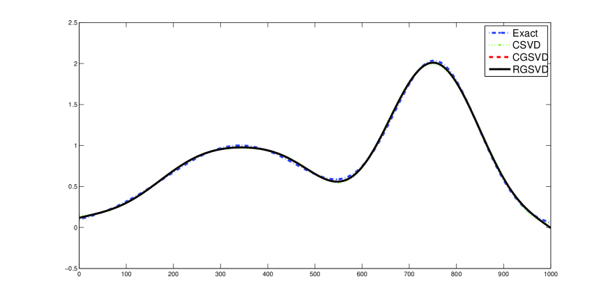
Figure 1: Shaw matrix of size $n=1000$.

CSVD CGSVD RGSVD $n$ $T(s)$ $\mu$ $err$ $T(s)$ $\mu$ $err$ $T(s)$ $\mu$ $err$ 500 0.46 4.59E-04 3.22E-02 0.47 1.00E-01 2.16E-02 0.06 1.00E-01 2.16E-02 1000 1.49 2.59E-04 2.74E-02 2.57 3.34E-01 1.89E-02 0.09 3.34E-01 1.89E-02 2000 9.73 2.59E-04 3.54E-02 20.6 1.21E-00 3.02E-02 0.19 1.21E-00 3.02E-02

Table 1: Comparison of the CPU time and solution accuracy among CSVD($L=I$), CGSVD and RGSVD.

Example 2 (I_laplace). This test problem is the inverse Laplace transformation, a Fredholm first kind integral equation, discretized by Gauss-Laguerre quadrature. The kernel $K$ is given by $K(s,t)=exp(-st)$.

Regularization Tools [10] provides the test problem I_laplace($n,eg$), with $n$ being the matrix size, and $eg=1,2,3$ or $4$ corresponds to four different examples. The test problem I_laplace($n$, 1) has the exact solution $x(t)=exp(-t/2)$, and I_laplace($n$, 3) gives $x(t)=t^{2}exp(-t/2)$. For these two cases, the solutions are smooth. The new method works very well with regularisation $L=tridiag(1,-1)$ and small sample size $l=50$. The accuracy is comparable or even better than that of the classical method using CGSVD, but the CPU times and memory requirements are essentially reduced. We do not report the numerical results for these two relatively easy cases, but focus on the other two cases, $eg=2$, $4$, which are more difficult due to the sudden change and strong discontinuity in the solutions. For these two cases, the regularization in general form (2) is necessary to ensure a meaningful numerical solution.

First for the test problem I_laplace($n$, 2), the exact solution is $x(t)=1-exp(-t/2)$, which has a horizontal asymptote. For this problem, the identity regularisation $L=I$ can not give a good reconstruction [13] (see Figure 2), and the regularisation $L=tridiag(1,-2,1)$ does not work well either. Instead, the regularisation $L=tridiag(1,-1)$ is very effective to capture the rapid change in the solution.

Let $e$ be the vector of all ones, i.e., $e=ones(n,1)$. Clearly $e$ is the basis vector of the null space of operator $L=tridiag(1,-1)$. This suggests us to incorporate a constant mode into the matrix $W$ in Algorithm 3. Suppose we have the approximate SVD of the matrix $A$ by randomized algorithm. That is, $A\approx U\Sigma W^{T}$. Let $w=(I-WW^{T})e$, then we enlarge the matrix $W$ by adding one more column vector, namely ${w}/{||w||}$. This is equivalent to finding the orthogonal projection onto $span\{W\}^{\perp}$, then adding it to matrix $W$ as a new column.

For most of our cases, the sample size can be as small as 50. But for this difficult case, we need to use larger size of samples. Even with larger sample size, the computational time of the new method is still much less than the traditional method, and the approximate solution is still quite accurate, actually the accuracy of the new method is much better than the traditional method; see Figure 2 and Table 2 for more details.

We observe from all the examples we have tested, our method working on a much smaller-sized problem is often more robust and stable than the classical method using CGSVD. This is also clearly observed in our test with I_laplace($n$, 4) from Regularization Tools [10]. The exact solution to the problem has a big jump:

$$x(t)=\left\{\begin{matrix}0,\quad t\leq 2;\\ 1,\quad t>2.\end{matrix}\right.$$

We choose the regularisation $L=tridiag(1,-1)$. We have observed that the traditional method using CGSVD fails mostly when we run the same test with different random noise in the data (right-hand side), but the new method using RGSVD always succeeds and achieves much better accuracy and requires much less time than the traditional method, even though we work on an approximate problem of much smaller size; see more details in Figure 3 and Table 3.

We remark that the truncated version of RGSVD also works quite well for the examples. Since the results are similar to the ones by Tikhonov regularization, we do not show any results by TGSVD in this work.

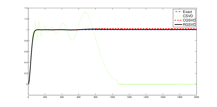
Figure 2: I_laplace($n$,2) matrix of size $n=2000$.

CSVD CGSVD RGSVD $n$ $T(s)$ $\mu$ $err$ $T(s)$ $\mu$ $err$ $T(s)$ $\mu$ $err$ 500 0.44 2.15E-04 7.59E-01 0.47 2.34E-02 5.10E-03 0.21 1.60E-01 1.50E-03 1000 1.56 1.18E-04 7.56E-01 3.59 1.26E-01 7.40E-03 1.34 2.47E-01 1.80E-03 2000 8.76 2.43E-04 7.45E-01 18.2 1.89E-01 1.71E-02 5.98 4.30E-01 5.50E-03

Table 2: I_Laplace($n$,2). Comparison of the CPU time and solution accuracy among CSVD($L=I$), CGSVD and RGSVD, with sample sizes $l=$ 150, 300, 600 respectively.

Figure 3: I_laplace($n$,4) matrix of size $n=1000$.

CSVD CGSVD RGSVD $n$ $T(s)$ $\mu$ $err$ $T(s)$ $\mu$ $err$ $T(s)$ $\mu$ $err$ 500 0.41 8.31E-05 7.56E-01 0.47 6.75E-04 4.43E-01 0.20 2.44E-01 4.94E-02 1000 1.27 2.52E-04 7.49E-01 2.50 2.20E-03 3.49E-01 0.99 2.56E-01 3.90E-02 2000 8.34 1.66E-04 7.45E-01 19.0 3.80E-03 2.53E-01 5.41 2.50E-01 3.22E-02

Table 3: I_Laplace($n$,4). Comparison of the CPU time and solution accuracy among CSVD($L=I$), CGSVD and RGSVD, with sample sizes $l=$ 150, 300, 600 respectively.

Example 3 (Foxgood). This example arises from discretization of the integral equation (25) with the kernel $K(s,t)=(s^{2}+t^{2})^{\frac{1}{2}}$ and the exact solution $x(t)=t$ [10].

The numerical results can be found in Figure 4 and Table 4. Similar conclusions and observations can be drawn for this example and the remaining 3 examples as for Example 1, so we will not repeat them. The CPU times and the solution accuracy clearly demonstrate the advantages of the new method.

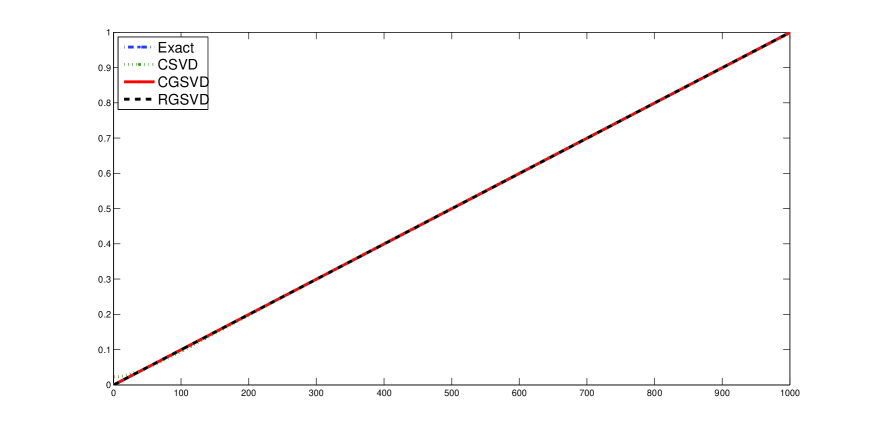
Figure 4: Foxgood matrix of size $n=1000$.

CSVD CGSVD RGSVD $n$ $T(s)$ $\mu$ $err$ $T(s)$ $\mu$ $err$ $T(s)$ $\mu$ $err$ 500 0.50 2.66E-04 8.30E-03 0.48 7.03E+01 3.09E-04 0.07 1.41E+02 1.25E-04 1000 1.59 4.71E-04 5.00E-03 2.54 2.81E+02 1.40E-04 0.10 3.90E+05 1.73E-05 2000 9.42 2.66E-04 2.70E-03 18.9 1.12E+03 1.77E-04 0.21 1.35E+03 1.45E-04

Table 4: Foxgood. Comparison of the CPU time and solution accuracy among CSVD($L=I$), CGSVD and RGSVD.

Example 4 (Gravity). This example arises from discretization of the equation (25) with the kernel $K(s,t)=d[d^{2}+(s-t)^{2}]^{-\frac{3}{2}}$, a one-dimensional model problem in gravity surveying. Here $d$ is the depth of the point source and controls the decay of the singular values [10].

The numerical results are given in Figure 5 and Table 5, when we take $d=0.25$ and the exact solution $x(t)=\sin(\pi t)+0.5\sin(2\pi t)$.

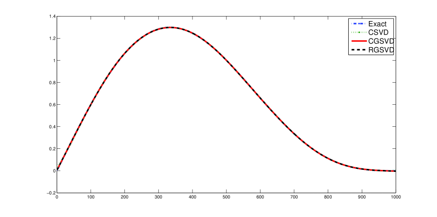
Figure 5: Gravity matrix of size $n=1000$.

CSVD CGSVD RGSVD $n$ $T(s)$ $\mu$ $err$ $T(s)$ $\mu$ $err$ $T(s)$ $\mu$ $err$ 500 0.40 5.80E-03 5.10E-03 0.44 9.69E+00 1.30E-03 0.07 9.69E+00 1.30E-03 1000 1.32 4.10E-03 4.60E-03 2.52 1.90E+01 7.26E-04 0.09 1.90E+01 7.26E-04 2000 9.29 4.00E-03 4.90E-03 18.5 6.69E+01 1.20E-03 0.19 6.69E+01 1.20E-03

Table 5: Gravity. Comparison of the CPU time and solution accuracy among CSVD($L=I$), CGSVD and RGSVD.

Example 5 (Heat). This example is the discretization of a Volterra integral equation of the first kind with the kernel $K(s,t)=k(s-t)$, where $k(t)=\frac{t^{-2/3}}{2\sqrt{\pi}}exp(-\frac{1}{4t})$; see [10] for more detail. The numerical results are given in Figure 6 and Table 6.

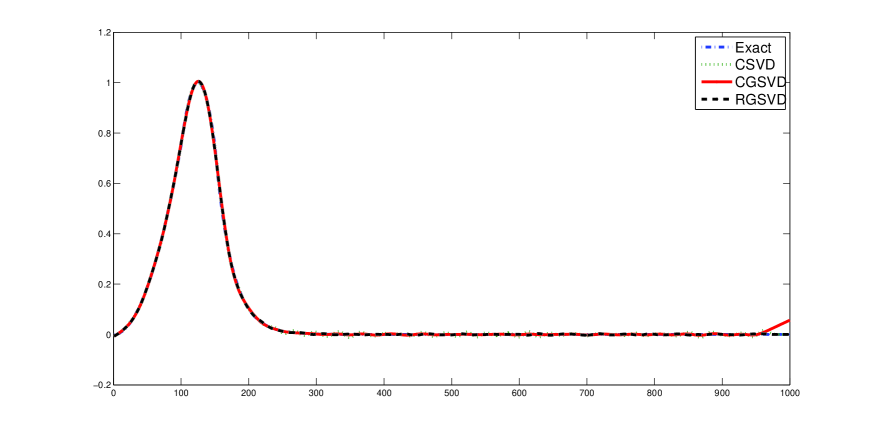
Figure 6: Heat matrix of size $n=1000$.

CSVD CGSVD RGSVD $n$ $T(s)$ $\mu$ $err$ $T(s)$ $\mu$ $err$ $T(s)$ $\mu$ $err$ 500 0.46 1.41E-04 1.62E-02 0.48 4.00E-03 3.67E-02 0.06 2.90E-03 1.59E-02 1000 1.79 7.97E-05 2.23E-02 2.59 1.03E-02 3.14E-02 0.09 1.11E-02 1.19E-02 2000 9.53 1.17E-04 1.23E-02 18.7 4.14E-02 1.32E-02 0.19 1.31E-02 1.57E-02

Table 6: Heat. Comparison of the CPU time and solution accuracy among CSVD($L=I$), CGSVD and RGSVD.

Example 6 (Phillips). This last testing problem arises from the discretization of the Fredholm integral equation of the first kind (25) designed by D. L. Phillips; see [10] for more detail. The numerical results are given in Figure 7 and Table 7.

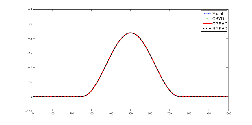
Figure 7: Phillips matrix of size $n=1000$.

CSVD CGSVD RGSVD $n$ $T(s)$ $\mu$ $err$ $T(s)$ $\mu$ $err$ $T(s)$ $\mu$ $err$ 500 0.51 8.70E-03 4.00E-03 0.49 1.24E-00 3.00E-03 0.06 1.15E-00 2.80E-03 1000 1.59 6.40E-03 5.40E-03 2.89 2.88E-00 3.20E-03 0.09 2.71E-00 2.90E-03 2000 10.7 5.30E-03 4.40E-03 20.3 8.76E-00 2.60E-03 0.19 7.68E-00 2.22E-03

Table 7: Phillips. Comparison of the CPU time and solution accuracy among CSVD($L=I$), CGSVD and RGSVD.

5 Conclusion

We have considered the randomized algorithms for the solutions of discrete ill-posed problems in general form. Several strategies are discussed to transform the problem of general form into the standard one, then the randomized strategies in [17] can be applied. The second approach we have proposed is to work on the problem of general form directly. We first reduce the original large-scale problem essentially by using the randomized algorithm RGSVD, so flops and memory are significantly saved. Our numerical experiments show that, using RGSVD we can still achieve the approximate regularized solutions of the same accuracy as the classical GSVD, but gain obvious robustness, stability and computational time as we need only to work on problems of much smaller size.

References

• [1] H. Banks and K. Kunisch, Parameter Estimation Techniques for Distributed Systems, 1989, Boston, MA: Birkhauser.
• [2] R. H. Chan and X. Q. Jin, An Introduction to Iterative Toeplitz Solvers, SIAM, 2007.
• [3] D. Colton and R. Kress, Inverse Acoustic and Electromagnetic Scattering Theory, 1998, 2nd edn, Berlin: Springer.
• [4] J. Demmel, L. Grigori, M. Hoemmen, and J. Langou, Communication-optimal parallel and sequential QR and LU factorizations, SIAM J. Sci. Comp. 34 (2012), pp. A206-A239.
• [5] J. Demmel, L. Grigori, M. Gu, and H. Xiang, Communication avoiding rank revealing QR factorization with column pivoting, LAPACK Working Note #276, May 2013, see also Technical Report No. UCB/EECS-2013-46, to appear in SIAM J. Matrix Anal. Appl.
• [6] L. Elden, Algorithms for the regularization of ill-conditioned least squares problems, BIT, 17 (1977), 134-145.
• [7] H. W. Engl, M. Hanke and A. Neubauer, Regularization of Inverse Problems, 1996, Dordrecht: Kluwer.
• [8] G. H. Golub and C. F. Van Loan, Matrix Computations, 4th edn, John Hopkins University Press, Baltimore, 2013.
• [9] N. Halko, P. Martinsson and J. Tropp, Finding structures with randomness: probabilistic algorithms for constructing approximate matrix decompositions, SIAM Rev. 53 (2011), pp. 217-88.
• [10] P. C. Hansen, Regularization tools: A Matlab package for analysis and solution of discrete ill-posed problems, Numer. Algorithms, 6 (1994), pp. 1-35. Software is available in Netlib at the web site http://www.netlib.org.
• [11] P. C. Hansen, Rank Deficient and Discrete Ill-Posed Problems, SIAM, Philadelphia, 1998.
• [12] P. C. Hansen, Discrete Inverse Problems: Insight and Algorithms, SIAM, Philadelphia, 2010.
• [13] P. C. Hansen, Oblique projections and standard-form transformations for discrete inverse problems, Numer. Lin. Algebra Appl. 20 (2013), pp. 250-258.
• [14] J. W. Ruge and K. StΓΌben, Algebraic multigrid (AMG), in Multigrid Methods, ed.. S. F. McCormick, volume 3 of Frontiers in Applied Mathematics. SIAM. Philadelphia, PA. (1987), pp. 73-130.
• [15] Sabine Van Huffel and Joos Vandewalle, The Total Least Squares Problem: Computational Aspects and Analysis, SIAM, Philadelphia, PA, 1991.
• [16] C. Van Loan, Computing the CS and the generalized singular value decompositions, Numer. Math. 46 (1985), pp. 479-491.
• [17] H. Xiang and J. Zou, Regularization with randomized SVD for large-scale discrete inverse problems, Inverse Problem 29 (2013), 085008.