Sudden death of particle-pair Bloch oscillation and unidirectioanl propagation in a one-dimensional driven optical lattice

Abstract

We study the dynamics of bound pairs in the extended Hubbard model driven by a linear external field. It is shown that the two interacting bosons or singlet fermions with nonzero on-site and nearest-neighbor interaction strengths can always form bound pairs in the absence of the external field. There are two bands of bound pair, one of which may have incomplete wave vectors when it has a overlap with the scattering band, referred as imperfect band. In the presence of the external field, the dynamics of the bound pair in the perfect band exhibits distinct Bloch-Zener oscillation (BZO), while in the imperfect band the oscillation presents a sudden death. The pair becomes uncorrelated after the sudden death and the BZO never comes back. Such dynamical behaviors are robust even for the weak coupling regime and thus can be used to characterize the phase diagram of the bound states.

I Introduction

The dynamics of particle-pair in lattice systems has received a lot of interest, due to the rapid development of experiment. Ultra-cold atoms have turned out to be an ideal playground for testing few-particle fundamental physics since optical lattices provide clean realizations of a range of many-body Hamiltonians. It stimulates many experimental Winkler ; Folling ; Gustavsson  and theoretical investigations in strongly correlated systems, which mainly focus on the bound-pair formation Mahajan ; Valiente2 ; MVExtendB ; MVTB ; Javanainen ; Wang , detection Kuklov , dynamics Petrosyan ; Zollner ; ChenS ; Valiente1 ; Wang ; JLNJP ; Corrielli , collision between single particle and pair JLBP ; JLTrans , and bound-pair condensate Rosch . The essential physics of the proposed bound pair (BP) is that, the periodic potential suppresses the single particle tunneling across the barrier, a process that would lead to a decay of the pair. This situation cannot be changed in general case when a weak linear potential is applied. Then a BP acts as a single particle, sharing the single-particle dynamical features, such as Bloch oscillation (BO), Bloch-Zener oscillation (BZO) MUGA ; Poladian ; Greenberg ; Kulishov ; Ruschhaupt ; Longhi2012 .

The aim of this paper is to show that the nearest-neighbor (NN) interaction can not only lead to distinct BO and BZO, but also induce the sudden death of the oscillations within a Bloch period. We study the dynamics of BPs in the extended Hubbard model driven by a linear external field. It is shown that two interacting bosons or singlet fermions with nonzero on-site and nearest-neighbor interaction strengths can always form BPs in the absence of the external field. There are two kinds of BP, which forms two bound bands. We find that the existence of the nearest-neighbor interaction can lead to the overlap between the scattering band of a single particle and the bound band, which can spoil the completeness of the bound band, referred as imperfect band. In the presence of the external field, the dynamics of the BP in the perfect band exhibits perfect BO and BZO, while in the imperfect band the oscillation presents a sudden death. The pair becomes uncorrelated after the sudden death of the oscillation and the correlation never come back. This behavior is of interest in both fundamental and application aspects. It can be utilized to control the unidirectional propagation of the BP wavepacket by imposing a single pulse, which is of great interest for applications in cold atom physics. Numerical simulations are shown that this scheme achieves very high efficiency and wide spectral band. Such a unidirectional filter for cold-atom pair may be realized in a shaking optical lattice in experiment.

This paper is organized as follows. In Section II, we present the model Hamiltonian, and the two-particle band structures. In Section III, we investigate the BP dynamics in the presence of linear field. Section IV is devoted to the application of our finding, the realization of unidirectional propagation induced by a pulsed field. Finally, we give a summary and discussion in Section V.

II Model Hamiltonian and band structure

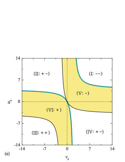
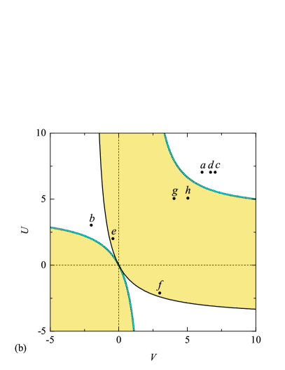
Figure 1: (Color online) (a) Phase diagram for the BP states. The solid black (blue) line is the hyperbolic function in Eq. (10), which is the boundary between the transition from the BP state $\left|\psi_{k}^{+}\right\rangle$ ($\left|\psi_{k}^{-}\right\rangle$) to a scattering state in each invariant subspace indexed by $k$. There are six regions divided by the lines from Eq. (10), where $\pm$ indicates the types of bound states $\left|\psi_{k}^{\pm}\right\rangle$ in each regions. (b) Phase diagram (in unit of $\kappa$) indicates the feature of the BP band: complete band in regions I-IV, while incomplete band in regions V and VI. Points $a\left(7,6\right)$, $b\left(3,-2\right)$, $c\left(7,7\right)$, $d\left(7,6.7\right)$, $e\left(2,-0.6\right)$, $f\left(-2,3\right)$ , $g\left(5,4\right)$ and $h\left(5,5\right)$ denote typical cases in each phases. The band structures and dynamical features in these cases are presented in Fig. 2 and 3.

We consider an extended Hubbard model describing interacting particles in the lowest Bloch band of a one dimensional lattice driven by an external force, which can be employed to describe ultracold atoms or molecules with magnetic or electric dipole-dipole interactions in optical lattices. We focus on the dynamics of the BP states. The pair can be two identical bosons, or equivalently, spin-$1/2$ fermions in singlet state. For simplicity we will only consider bosonic systems, but it is straightforward to extend the conclusion to singlet fermionic pair. We consider the Hamiltonian

$$H=H_{0}+F\sum_{j=1}jn_{j},$$ (1)

where the second term describes the linear external field while $H_{0}$ is one-dimensional Hamiltonian for the extended Bose-Hubbard model on a $N$-site lattice

$$H_{0}=-\kappa\sum_{j=1}\left(a_{j}^{\dagger}a_{j+1}+\textrm{H.c.}\right)+\frac{U}{2}\sum_{j=1}n_{j}\left(n_{j}-1\right)+V\sum_{j=1}n_{j}n_{j+1}.$$ (2)

where $a_{i}^{{\dagger}}$ is the creation operator of the boson at the $i$th site, the tunneling strength, on-site and NN interactions between bosons are denoted by $\kappa$, $U$ and $V$.

Let us start by analyzing in detail the two-boson problem in this model. As in Refs. JLNJP ; JLBP ; JLTrans , a state in the two-particle Hilbert space, can be expanded in the basis set $\left\{\left|\phi_{r}^{k}\right\rangle,r=0,1,2,...\right\}$, with

$$\left|\phi_{0}^{k}\right\rangle = \frac{1}{\sqrt{2N}}\sum_{j}e^{ikj}\left(a_{j}^{{\dagger}}\right)^{2}\left|\textrm{vac}\right\rangle,$$ (3)

$$\left|\phi_{r}^{k}\right\rangle = \frac{1}{\sqrt{N}}e^{ikr/2}\sum_{j}e^{ikj}a_{j}^{{\dagger}}a_{j+r}^{{\dagger}}\left|\textrm{vac}\right\rangle,$$ (4)

where $\left|\textrm{vac}\right\rangle$ is the vacuum state for the boson operator $a_{i}$. Here $k$ denotes the momentum, and $r$ is the distance between the two particles. Due to the translational symmetry of the present system, we have the following equivalent Hamiltonian

$$H_{\mathrm{eq}}^{k}=-J_{k}(\sqrt{2}\left|\phi_{0}^{k}\right\rangle\left\langle\phi_{1}^{k}\right|+\sum_{j=1}\left|\phi_{j}^{k}\right\rangle\left\langle\phi_{j+1}^{k}\right|+\textrm{H.c.)}+U\left|\phi_{0}^{k}\right\rangle\left\langle\phi_{0}^{k}\right|+V\left|\phi_{1}^{k}\right\rangle\left\langle\phi_{1}^{k}\right|$$ (5)

in each invariant subspace indexed by $k$. In its present form, $H_{\mathrm{eq}}^{k}$ are formally analogous to the tight-binding model describing a single-particle dynamics in a semi-infinite chain with the $k$-dependent hopping integral $J_{k}=2\kappa\cos\left(k/2\right)$ in thermodynamic limit $N\rightarrow\infty$. In this paper, we are interested in the BP states, which corresponds to the bound state solution of the single-particle Schrödinger equation

$$H_{\mathrm{eq}}^{k}\left|\psi_{k}\right\rangle=\epsilon_{k}\left|\psi_{k}\right\rangle.$$ (6)

For a given $J_{k}$, the Hamiltonian $H_{\mathrm{eq}}^{k}$ possesses one or two bound states, which are denoted as $\left|\psi_{k}^{+}\right\rangle$ and $\left|\psi_{k}^{-}\right\rangle$, respectively. Here the Bethe-ansatz wavefunctions have the form

$$\left|\psi_{k}^{\pm}\right\rangle=C_{0}^{k}\left|\phi_{0}^{k}\right\rangle+\sum_{r=1}\left(\pm 1\right)^{r}C_{r}^{k}e^{-\beta r}\left|\phi_{r}^{k}\right\rangle,$$ (7)

with $\beta>0$. For such two bound states $\left|\psi_{k}^{\pm}\right\rangle$ the Schrodinger equation in Eq. (6) admits

$$\pm e^{3\beta}+\left(u_{k}+v_{k}\right)e^{2\beta}\pm\left(u_{k}v_{k}-1\right)e^{\beta}+v_{k}=0,$$ (8)

where $u_{k}=U/J_{k}$ and $v_{k}=V/J_{k}$ are respectively the reduced interaction strengthes. The corresponding bound-state energy of $\left|\psi_{k}^{\pm}\right\rangle$ can be expressed as

$$\epsilon_{k}^{\pm}=\pm J_{k}\cosh\beta.$$ (9)

The transition from bound to scattering states occurs at $\beta=0$. Then the boundary, at which the bound state $\left|\psi_{k}^{\pm}\right\rangle$ disappears, is described by the hyperbolic function

$$u_{k}=-\frac{2v_{k}}{1\pm v_{k}},$$ (10)

which is plotted in Fig. 1. It shows that the boundary lines divide the $u_{k}-v_{k}$ plane into six regions, from $\mathrm{I}$ to $\mathrm{VI}$. The type of the bound states in each region can be foreseen from the extreme situations where $\left|u_{k}\right|,$ $\left|v_{k}\right|\gg 1$. Under this condition, it is easy to check that there are two bound states with the eigen energies

$$\epsilon_{k}^{\pm}\approx U\textrm{ and }V,$$ (11)

in each invariant $k$-subspace. Comparing Eqs. (11) and (9), we get the conclusion that there are two bound states in the regions $\mathrm{I}$, $\mathrm{II}$, $\mathrm{III}$, and $\mathrm{IV}$: two $\left|\psi_{k}^{-}\right\rangle$ in $\mathrm{I}$, one $\left|\psi_{k}^{+}\right\rangle$ and $\left|\psi_{k}^{-}\right\rangle$ in $\mathrm{II}$ and $\mathrm{IV}$, two $\left|\psi_{k}^{+}\right\rangle$ in $\mathrm{III}$, while there is a bound state $\left|\psi_{k}^{-}\right\rangle$ in $\mathrm{V}$ and $\left|\psi_{k}^{+}\right\rangle$ in $\mathrm{VI}$, respectively.

On the other hand, we know that the scattering band of $H_{\mathrm{eq}}^{k}$ ranges from $-4\kappa\cos\left(k/2\right)$ to $4\kappa\cos\left(k/2\right)$, which reaches the widest bandwidth at $k=0$. Therefore, when we take $J_{0}=\pm 2\kappa$, this diagram can characterize the bound-state number distribution $N_{\mathrm{b}}(U,V)$: we have $N_{\mathrm{b}}=2N$ in the regions $\mathrm{I}$, $\mathrm{II}$, $\mathrm{III}$, and $\mathrm{IV}$, where all the $2N$ bound states indexed by $k$ constitute a complete BP band. In contrast, we have $N_{\mathrm{b}}<2N$ in $\mathrm{V}$ and $\mathrm{VI}$, where all $N_{\mathrm{b}}$ bound states indexed by survival $k$, which does not cover all range of the momentum in the Brillouin zone, from $-\pi$ to $\pi$. We refer to this property as incomplete BP band. Therefore, the phase diagram also indicates the boundary $U=-2V/\left(1\pm V\right)$, for the transition from the complete to incomplete BP bands, which agrees with the results reported in Refs. Valiente2009 ; Dias ; Khomeriki . For given $U$ and $V$, the complete spectrum of $H_{0}$ can be computed by diagonalizing the Hamiltonian $H_{\mathrm{eq}}^{k}$ numerically. In Fig. 2 and 3, we plot the band structures for several typical cases, which are marked in Fig. 1. We do not cover all the typical points in every region due to the following fact. The spectrum of $H_{0}$ obeys the relation

$$E_{k}\left(U,V\right)=-E_{k}\left(-U,-V\right),$$ (12)

in view of

$$H_{0}(U,V)=-RH_{0}(-U,-V)R^{-1},$$ (13)

where the transformation $R$ is defined as $Ra_{j}R^{-1}=\left(-1\right)^{j}a_{j}$. It is a rigorous result in the all range of the parameters. As expected, we observe that the two-particle spectrum comprises three Bloch bands, two BP bands formed by two kinds of BP states, and one scattering band formed by uncorrelated states. We can see from the Fig. 2, that two bound bands are separated from the scattering band whenever the system is in the regions (points $a$, $b$, $c$ and $d$) $\mathrm{I}$, $\mathrm{II}$, $\mathrm{III}$, and $\mathrm{IV}$. In contrast, whenever the points ($e$, $f$, $g$ and $h$) lie in the regions $\mathrm{V}$ and $\mathrm{VI}$, the pseudo gap between BP and scattering bands around $k=0$ vanishes, resulting the formation of incomplete band. What it quite unexpected and remarkable is that if we apply a linear field, the dynamics of the BP exhibits some peculiar behaviors, which will be investigated in the following section.

III BP dynamics

Before starting the investigation of the BP dynamics, we would like to study the relation between the center path of a wavepacket driven by the linear field and dispersion of the Hamiltonian $H_{0}$. Consider a general one-dimensional tight-binding system, which has the dispersion relation $E(k)$ being an arbitrary smooth periodic function $E(2\pi+k)=E(k)$. The dynamics of wavepacket can be simply understood in terms of the semiclassical picture: A wavepacket centered around $k_{\mathrm{c}}$ can be regarded as a classical particle with momentum $k_{\mathrm{c}}$ Bloch ; Ashcroft ; Kittel . When the wavepacket is subjected to a homogeneous force of strength $F$, the acceleration theorem $\partial k_{\mathrm{c}}\left(t\right)/\partial t=F$ tells us

$$k_{\mathrm{c}}\left(t\right) = k_{\mathrm{c}}\left(0\right)+\int_{0}^{t}Fdt$$ (14)

$$= k_{\mathrm{c}}\left(0\right)+Ft$$

for constant field. The central position of the wavepacket is

$$x_{\mathrm{c}}\left(t\right) = x_{\mathrm{c}}\left(0\right)+\int_{0}^{t}\upsilon_{\mathrm{g}}dt$$ (15)

$$= x_{\mathrm{c}}\left(0\right)+\frac{1}{F}\left[E_{k}\left(k_{\mathrm{c}}\left(0\right)+Ft\right)-E_{k}\left(k_{\mathrm{c}}\left(0\right)\right)\right]$$

where $\upsilon_{\mathrm{g}}=\partial E_{k}/\partial k$ is the group velocity. Notice that the trajectory of a wavepacket is essentially identical with the dispersion relation for the field-free system under the semi-classical approximation. This observation provides a fairly clear picture for the dynamics of a wavepacket in the presence of the linear field. As a simple example we consider a single-particle case for illustration. The single-particle BO with Bloch frequency $\omega_{\mathrm{B}}=F$ for $H$ can be simply understood from its cosusoidal dispersion relation $E(k)=-2\kappa\cos k$ rather than quadratic, in momentum $k$.

Now, we switch gears to the case of two-particle. We note that the bandwidth of the BP band is comparable to that of scattering band, which leads to the conclusion that a BP wavepacket has distinct group velocity. It indicates that the dynamics of the BP state has the similar behavior with the single particle. The BO-like behavior of the BP wavepacket emerges in the presence of the linear external field.

In order to demonstrate these points, we consider an example for the Hamiltonian $H$ in Eq. (1) with $U$, $V\gg\left|U-V\right|$, $\kappa$. As studied in Ref. JLNJP , in the absence of the external field, the BP lies in the quasi-invariant subspace spanned by the basis $\{\underline{\left|l\right\rangle}\}$, which is defined as

$$\underline{\left|l\right\rangle}\equiv\left\{\begin{array}[]{c}\left(a_{l/2}^{{\dagger}}\right)^{2}/\sqrt{2}\left|\textrm{vac}\right\rangle\textrm{, }(\textrm{even }l)\\ a_{\left(l-1\right)/2}^{{\dagger}}a_{\left(l+1\right)/2}^{{\dagger}}\left|\textrm{vac}\right\rangle\textrm{,\ }(\textrm{odd }l)\end{array}\right..$$ (16)

In the presence of the external field, the bound-pair can be described by the following effective Hamiltonian

$$H_{\mathrm{eff}}=-\sqrt{2}\kappa\sum\limits_{l}\left(\underline{\left|l\right\rangle}\underline{\left\langle l+1\right|}+\textrm{H.c.}\right)+\sum\limits_{l}\left[Fl+\frac{\delta}{2}\left(-1\right)^{l}\right]\underline{\left|l\right\rangle}\underline{\left\langle l\right|},$$ (17)

where we neglect a constant term $\left(U+V\right)/2\sum_{l}\underline{\left|l\right\rangle}\underline{\left\langle l\right|}$ and  take $\delta=U-V$ to present the unbalanced on-site and nearest neighbor interactions. $H_{\mathrm{eff}}$ is nothing but the tight-binding Hamiltonian to describe a single particle subjected to a staggered linear potential, which has been well studied in previous literature Breid . Unlike the fractional BO Buchleitner ; Kolovsky ; Kudo2009 ; Kudo2011 in the case of $V=0$, $H_{\mathrm{eff}}$ can support wide bandwidth JLNJP , which is responsible for the large amplitude oscillations. In the situation with $\delta=0$, it turns out that particle undergoes BO with frequency $\omega_{\mathrm{B}}=F$. In the case of nonzero unbalance $\delta\neq 0$, it has been reported that the dynamics of the wavepacket shows a BZO, a coherent superposition of Bloch oscillations and Zener tunnelling between the sub-bands. The Zener tunnelling takes place almost exclusively when the momentum of wavepacket reaches $\pm\pi$. Then we get the conclusion that the BPs serve as a composite particle, exhibiting BO and BZO in strong coupling region.

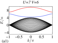
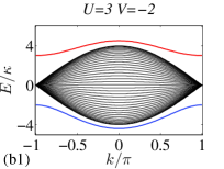
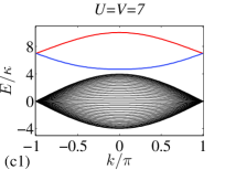
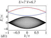
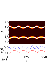
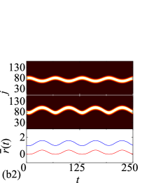
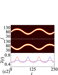
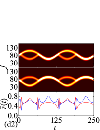
Figure 2: (Color online) (a1-d1) The band structures for the systems with parameters fixed at the typical points ($a$-$d$) labelled in Fig. 1. All the BP bands are complete. (a2-d2) The profiles and the average distances $\bar{r}\left(t\right)$ of the time evolution of the initial wavepackets in the form of Eq. (19) with $k_{0}=-0.8\pi$, $\alpha=0.15$, and $N_{\mathrm{A}}=80$, of the two BP bands, in the external field with $F_{0}=0.05$, in which the time $t$ is expressed in units of $1/\kappa$. We can see the perfect BO and BZO phenomenon. The evolution of $\bar{r}\left(t\right)$ shows that the correlation of the BP remains strong.

In this paper we are interested in what happens if the initial state is placed in a incomplete band. It is presumable that the semi-classical theory still holds when the wavepacket is in the extent of the in incomplete band, because the nonzero pseudogap can protect the BP wavepacket from the scattering band. However, when the wavepacket reaches the band edge, the transition from bound to the scattering band occurs. The wavepacket diffuses into the continuous spectrum rather than the repetitive motion of acceleration and Bragg reflection. We refer to this phenomenon as the sudden death of the BO. In the case of the incomplete BP band with a edge $k_{\mathrm{m}}>0$, the life time $\tau$ for an initial wavepacket with $k_{\mathrm{c}}\left(0\right)$ satisfies

$$k_{\mathrm{m}}=\left|k_{\mathrm{c}}\left(0\right)+\tau F\right|.$$ (18)

When this occurs, the correlation between two particles breaks down and the wavepacket spreads out in space, irreversibly.

To verify and demonstrate the above analysis, numerical simulations are performed to investigate the dynamics behavior. We compute the time evolution of the wavepacket by diagonalizing the Hamiltonian $H$ numerically. Throughout this paper, we investigate the dynamics of the initial Gaussian wavepacket in the form

$$\left|\Psi\left(0\right)\right\rangle=\Lambda\sum_{k}\exp\left[-\frac{\left(k-k_{0}\right)^{2}}{2\alpha^{2}}-iN_{\mathrm{A}}\left(k-k_{0}\right)\right]\left|\psi_{k}\right\rangle,$$ (19)

where $\Lambda$ is the normalization factor, $k_{0}$ and $N_{\mathrm{A}}$ denote the central momentum and position of the initial wavepacket, respectively. The evolved state under the Hamiltonian $H$ is $\left|\Psi\left(t\right)\right\rangle$ = $e^{-iHt}\left|\Psi\left(0\right)\right\rangle$. We would like to stress that the initial wavepacket involves solely one BP band, either upper or lower one. However, the evolved state may involve two BP bands, even the scattering band, when the Zener tunnelling occurs. We plot the probability profile of the wavepacket evolution in several typical cases in Fig. 2 and 3. In Fig. 2, the simulation is performed in the systems, where two bound bands are well separated from the scattering band. As the external field is turned on, several dynamical behaviors occur: when two bound bands are well separated ($a1$ and $b1$), the BOs in both bands are observed ($a2$ and $b2$). In the case ($d1$, $d2$), two bound bands are very close at $\pm\pi$, which induces the BZO as expected. For the three cases, the BO frequency doubles comparing with that of single particle case. Case ($c1$, $c2$) fixes $U=V$, two bound bands merg into a single bound band. As predicted above, simple BO rather than BZO is observed, with a period equal to that of single-particle BO.

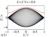
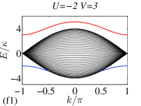
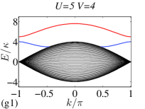
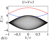
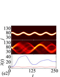
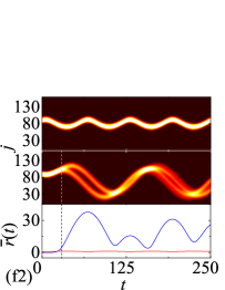
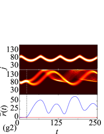
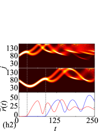
Figure 3: (Color online) The same as that in 2 but for the systems with parameters fixed at the typical points $e$-$f$ labelled in Fig. 1. It shows that the BP band becomes incomplete due to the overlap between the bound and scattering energy levels. We can see the sudden death of the BO, which closely accompanies the breakdown of the pair correlation. Here the time $t$ is also expressed in units of $1/\kappa$.

In Fig. 3, the systems have a common feature: one of the BP bands is incomplete due to the pseudo gap vanishing. In the three cases ($e2$, $f2$ and $g2$), the BOs remain in one band, whereas the BOs break down at the edges of the incomplete band. For the case ($h1$, $h2$) with $U=V$, two bound bands merg into a single incomplete band. The BP wavepackets in both two bands cannot survive from the irreversible spreading.

Furthermore, the correlation between two particles is measured by the average distance of two particle

$$\overline{r}\left(t\right)=\sum_{i,r}r\left\langle\Psi\left(t\right)\right|n_{i}n_{i+r}\left|\Psi\left(t\right)\right\rangle,$$ (20)

which can be used to characterize the feature of sudden death of BO for a evolved state $\left|\Psi\left(t\right)\right\rangle$. As comparison, the average distance $\overline{r}\left(t\right)$ as function of time for several typical cases is plotted in Fig. 2 and 3. We find that the sudden death of BO is always accompanied by the irreversible increasing of $\overline{r}\left(t\right)$, which accords with our analytical predictions.

Finally, we also plot the BP dispersion relation $E\left(k\right)$ and the central position $x_{\mathrm{c}}\left(t\right)$ of the wavepacket under the driving force together in one figure. For several typical cases, the plots in Fig. 4 indicate that the shape of the function $x_{\mathrm{c}}\left(t\right)$ coincides with that of the dispersion relation $E(k)$. We also find that the semi-classical analysis in Eq. (15) is valid if $\delta$ is not too small. Remarkably, one can see that such a relation still holds even for the incomplete BP band. These results are in agreement with the theoretical prediction based on the spectral structures.

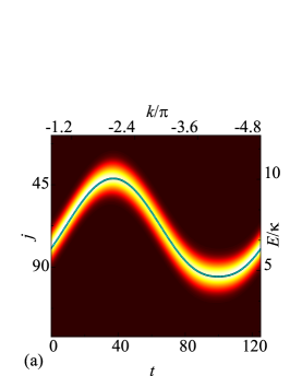
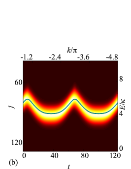
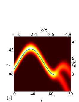
Figure 4: (Color online) The comparison between the BP dispersion relations and the central positions for the cases plotted in Fig. 2 and 3: (a) lower band in $c$; (b) lower band in $a$; (c) lower band in $h$. It shows that the two are in close proximity to each other even for the case of incomplete band, which corresonds to the sudden death of the BO. The time $t$ is expressed in units of $1/\kappa$.

IV Unidirectional propagation

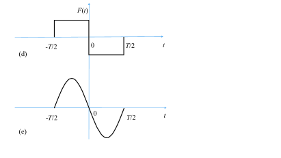
Figure 5: (Color online) Schematic illustration for the possess of realizing unidirectional propagation of BP. The dashed $\infty$ represents the correlation between two particles. The shaking lattice induces the inertial force $F\left(t\right)$. (a) for $t{<-T/2}$, bound-pair wavepacket moves towards to the right or left with constant group velocity. (b) during the period of time $[-T/2,T/2]$, a pulse field $F(t)$, is subjected to the pairs by shaking the lattice back and forth, which may break down the BP moving to the left. (c) after the time $T/2$, the surviving wavepacket goes back to its original state, while another pair is bounded back and becomes uncorrelated. (d) and (e) are two example forms of $F(t)$, which are taken for the numerical simulations in Fig. 6.

We now investigate the effect of the time-dependent driving force on the dynamics of a BP wavepacket. The acceleration theorem (14) tells us a pulsed field can shift the central momentum of the wavepacket in the case of complete band. However, it is easy to find that a pulsed field may destroy a BP wavepacket in the incomplete band, similarly referred as sudden death of uniform motion. The death and survival of a propagating wavepacket strongly depends on the difference between the initial central momentum and the edge of the incomplete band. Of course, a survived wavepacket can retain its original motion state by a subsequently compensating pulsed field. This gives rise to a scheme for destroying the pair wavepacket propagating in one direction, but remaining the one with the opposite direction. Such kind of scheme can be carried out by two pulsed fields in a pair of adjacent intervals, which provides two opposite impulses to the wavepacket.

To illustrate the scheme, we propose two concrete examples. The first one is a square-wave pulse driving force in the form

$$F\left(t\right)=\left\{\begin{array}[]{cc}F_{0},&-T/2<t\leq 0,\\ -F_{0},&0<t\leq T/2,\\ 0,&\textrm{otherwise,}\end{array}\right..$$ (21)

According to the acceleration theorem, an initial wavepacket with momentum $k_{c}\left(0\right)$ will acquire a momentum shift $F_{0}T/2$ at instant $t=0$ if $k_{\mathrm{c}}\left(0\right)+F_{0}T/2$ is within the band. The action of the subsequent force $-F_{0}$ can return the group velocity to the initial value, continue its motion in the same direction. However, in the case of $k_{\mathrm{c}}\left(0\right)+F_{0}T/2$ beyond the incomplete band, the BP wavepacket breaks down before $t=0$ and the subsequent force cannot get the correlation back. Therefore, for two BP wavepackets with opposite momenta $\pm k_{\mathrm{c}}\left(0\right)$ or group velocities $\pm\upsilon_{\mathrm{g}}\left(0\right)$, one can always choose a proper $F\left(t\right)$ to destroy one of them and maintain the other. This feature can be used to control the direction of wavepacket propagation in demand. Alternatively, one can also consider the sine-wave pulse driving force

$$F\left(t\right)=\left\{\begin{array}[]{cc}\left(-F_{0}\pi/2\right)\sin\left(2\pi t/T\right),&t\leq\left|T/2\right|,\\ 0,&\textrm{otherwise,}\end{array}\right.,$$ (22)

to achieve the same effect from Eq. (14). To examine how these schemes works in practice, we apply it to a wavepacket in the form of (19). Fig. 6 shows a numerical propagation of the Gaussian wavepacket under the action of two kinds of pulse driving forces. It shows that wavepackets with opposite group velocities exhibit entirely different behaviors: one remains the original motion state, while the other spreads out in space. Remarkably, the probability of the broken wavepacket is reflected by the pulsed field, which indicates that the unidirectional effect in the scheme works not only for the two-particle correlation but also for the probability flow. In addition, one can see a separation of slight portion from the moving wavepacket under the action of the square-wave pulsed field.

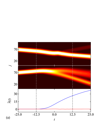
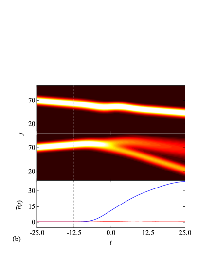
Figure 6: (Color online) The profiles and the avarage distances $\bar{r}\left(t\right)$ of the time evolution of the initial wavepackets in the form of Eq. (19) with $k_{0}=\pm 0.6\pi$, $\alpha=0.15$, and $N_{\mathrm{A}}=70,$ in the lower band of the system with $U=5$, $V=4,$ and $F_{0}=0.05$. The pulse field is taken as the forms of (a) square wave and (b) sine wave, respectively. We can see in both cases that, the wavepacket with $k_{0}=-0.6\pi$ is spread out by the pulse field, while the one with $k_{0}=0.6\pi$ remains the original motion state. Here the time $t$ is expressed in units of $1/\kappa$.

The probability flow of two particles, no matter correlated or not, can be depicted by the center of mass (COM)

$$x_{\mathrm{c}}\left(t\right)=\sum_{j}\left\langle jn_{j}\right\rangle_{t},$$ (23)

where $\left\langle...\right\rangle_{t}$ denotes the average for a evolved state. On the other hand, to characterize the efficiency of the schemes, we introduce the fidelity defined as

$$\mathcal{F} = \textrm{max}\left[f\left(t\right)\right],$$ (24)

$$f\left(t\right) = \left|\left\langle\Psi_{t}\left(t\right)\right|\left.\Psi_{0}\left(t_{0}\right)\right\rangle\right|,$$

where

$$\left|\Psi_{0}\left(t_{0}\right)\right\rangle=\exp(-iH_{0}t_{0})\left|\Psi\left(0\right)\right\rangle$$ (25)

is the target state and

$$\left|\Psi_{t}\left(t\right)\right\rangle=\mathcal{T}\exp(-i\int_{0}^{t}H\left(t\right)\mathrm{d}t)\left|\Psi\left(0\right)\right\rangle$$ (26)

is the transferred state subjected to a pulsed field. Here we have omitted a shift on the time scale comparing to the expression of $F\left(t\right)$. The computation is performed by using a uniform mesh in the time discretization for the time-dependent Hamiltonian $H\left(t\right)$. As an example, in Fig. 7, we show the evolution of the COM $x_{\mathrm{c}}\left(t\right)\$and the fidelity $f\left(t\right)$ for the same parameter values as the four processes simulated in Fig. 6. The plot in (a) shows the behavior of the two-particle transmission and reflection induced by the pulsed field, while in (b) the fidelities of the state transfer. It indicates that a sine-wave pulse has a higher fidelity ($\mathcal{F}=0.994$) than that of square-wave pulse ($\mathcal{F}=0.940$). These results clearly demonstrate the power of the mechanism proposed in this paper with the purpose to induce unidirectional propagation which is caused by a pulsed field.

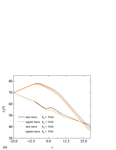
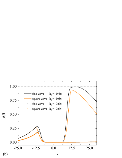
Figure 7: (Color online) Plots of the COM $x_{\mathrm{c}}\left(t\right)$ (a) and the fidelity $f\left(t\right)$ (b) for the process illustrated in Fig. 6, where the time $t$ is expressed in units of $1/\kappa$. (a) clearly shows that, the pulsed field bounces back one pair but maitains another. The gray dashed lines are drawn as guidance to eye indicating the initial and final paths for the case of sine wave. (b) indicates that the sine-wave pulse has very high efficiency for the control of unidirectional propagation.

It is easy to estimate the spectral band of the unidirectional filter by neglecting the width of the wavepacket. We find that there are three reasons that trigger the death of a propagating wavepacket: (i) the central momentum of the initial wavepacket, (ii) the edge of the incomplete band, which is determined by the values of $U/\kappa$ and $V/\kappa$, (iii) the impulse of the single pulsed field. We consider the lattice with one bound band just touching the scattering band at the center momentum $k=0$. We note, but do not prove exactly, that the dispersion relation in the left region $\left[-\pi,0\right]$ and right region $\left[0,\pi\right]$ are monotone functions. Then if we apply a pulsed field with impulse $\pi$, a moving wavepacket with the momentum in the left region should be pushed into the scattering band and will not be recovered by the subsequent $-\pi$ impulse. In contrast, a wavepacket in the right region still keep its initial situation after this process. Therefore, roughly speaking, the proposed unidirectional filter works for the wavepacket with all possible group velocity.

V Summary

In this paper, the coherent dynamics of two correlated particles in one-dimensional extended Hubbard model with on-site $U$ and nearest-neighbor site $V$ interactions, driven by a linear field has been theoretically investigated. The analysis shows that in the free-field case, there always exist BP states for any nonzero $U$ and $V$, which may have the comparable bandwidth with that of single particle. It results in the onset of distinct BO and BZO for correlated pair in the presence of the external field. We found that the incompleteness of the BP band spoils the correlation of the pair and leads to the sudden death of the BO and BZO. Based on this mechanism, we propose a scheme to control the unidirectional propagation of the BP wavepacket by imposing a single pulse. As a simple application of this scheme, we investigate the effect of two kinds of pulsed field. Numerical simulations indicate that a sine-wave pulse has a higher fidelity than that of square-wave pulse. In experiment, it has been proposed that the ultracold atomic gases in optical lattices with sinusoidal shaking can be an attractive testing ground to explore the dynamical control of quantum states Madison ; Gemelke ; Lignier ; Chen . The sudden death of BO predicted in this paper is an exclusive signature of correlated particle pair and could be applied to the quantum and optical device design.

References

References

- (1) K. Winkler, G. Thalhammer, F. Lang, R. Grimm, J. H. Denschlag, A. J. Daley, A. Kantian, H. P. Büchler, and P. Zoller, Nature (London) 441, 853 (2006).
- (2) S. Fölling, S. Trotzky, P. Cheinet, M. Feld, R. Saers, A. Widera, T. Müller, and I. Bloch, Nature (London) 448, 1029 (2007).
- (3) M. Gustavsson, E. Haller, M. J. Mark, J. G. Danzl, G. Rojas-Kopeinig, and H. C. Nägerl, Phys. Rev. Lett. 100, 080404 (2008).
- (4) S. M. Mahajan and A. Thyagaraja, J. Phys. A 39, L667 (2006).
- (5) M. Valiente and D. Petrosyan, J. Phys. B 41, 161002 (2008).
- (6) M. Valiente and D. Petrosyan, J. Phys. B 42, 121001 (2009).
- (7) M. Valiente, D. Petrosyan, and A. Saenz, Phys. Rev. A 81, 011601(R) (2010).
- (8) J. Javanainen, O. Odong, and J. C. Sanders, Phys. Rev. A 81, 043609 (2010).
- (9) Y. M. Wang and J. Q. Liang, Phys. Rev. A 81, 045601 (2010).
- (10) A. Kuklov and H. Moritz, Phys. Rev. A 75, 013616 (2007).
- (11) D. Petrosyan, B. Schmidt, J. R. Anglin, and M.Fleischhauer, Phys. Rev. A 76, 033606 (2007).
- (12) S. Zöllner, H.-D. Meyer, and P. Schmelcher, Phys. Rev. Lett. 100, 040401 (2008).
- (13) L. Wang, Y. Hao, and S. Chen, Eur. Phys. J. D 48, 229 (2008).
- (14) M. Valiente and D. Petrosyan, Europhys. Lett. 83, 30007 (2008).
- (15) L. Jin and Z. Song, New J. Phys. 13, 063009 (15pp) (2011).
- (16) G. Corrielli, A. Crespi, G. D. Valle, S. Longhi, and R. Osellame, Nat. Commun. 4, 1555 (2012).
- (17) L. Jin, B. Chen, and Z. Song, Phys. Rev. A 79, 032108 (2009).
- (18) L. Jin and Z. Song, Phys. Rev. A 81, 022107 (2010).
- (19) A. Rosch, D. Rasch, B. Binz, and M. Vojta, Phys. Rev. Lett. 101, 265301 (2008).
- (20) J. G. Muga, J. P. Palao, B. Navarro, and I. L. Egusquiza, Phys. Rep. 395, 357 (2004).
- (21) L. Poladian, Phys. Rev. E 54, 2963 (1996).
- (22) M. Greenberg and M. Orenstein, Opt. Lett. 29, 451 (2004).
- (23) M. Kulishov, J. M. Laniel, N. Belanger, J. Azana, and D. V. Plant, Opt. Express 13, 3068 (2005).
- (24) A. Ruschhaupt, J. G. Muga, and M. G. Raizen, J. Phys. B 39, 3833 (2006).
- (25) S. Longhi, Phys. Rev. B 86, 075144 (2012).
- (26) M. Valiente and D. Petrosyan, J. Phys. B: At. Mol. Phys. 42, 121001 (2009).
- (27) W. S. Dias, M. L. Lyra, and F. A. B. F. de Moura, Phys. Lett. A 374, 4554 (2010).
- (28) R. Khomeriki, D. O. Krimer, M. Haque, and S. Flach, Phys. Rev. A 81, 065601 (2010).
- (29) F. Bloch, Z. Phys. 52, 555 (1929).
- (30) N. W. Ashcroft and N. D. Mermin, Solid State Physics (Harcourt, Fort Worth), Chap. 12 (1976).
- (31) Kittel C, Quantum Theory of Solids, 2nd ed. (Wiley, New York) (1987).
- (32) B. M. Breid, D. Witthaut, and H. J. Korsch, New J. Phys. 8, 110 (2006).
- (33) A. Buchleitner and A. R. Kolovsky, Phys. Rev. Lett. 91, 253002 (2003).
- (34) A. R. Kolovsky, Phys. Rev. A 70, 015604 (2004).
- (35) K. Kudo, T. Boness, and T. S. Monteiro, Phys. Rev. A 80, 063409 (2009).
- (36) K. Kudo and T. S. Monteiro, Phys. Rev. A 83, 053627 (2011).
- (37) K. W. Madison, M. C. Fischer, R. B. Diener, Q. Niu, and M. G. Raizen, Phys. Rev. Lett. 81, 5093 (1998).
- (38) N. Gemelke, E. Sarajlic, Y. Bidel, S. Hong, and S. Chu, Phys. Rev. Lett. 95, 170404 (2005).
- (39) H. Lignier, C. Sias, D. Ciampini, Y. Singh, A. Zenesini, O. Morsch, and E. Arimondo, Phys. Rev. Lett. 99, 220403 (2007).
- (40) Y. A. Chen, S. Nascimbène, M. Aidelsburger, M. Atala, S. Trotzky, and I. Bloch, Phys. Rev. Lett. 107, 210405 (2011).