Is there a connection between Broad Absorption Line Quasars and Narrow Line Seyfert 1 galaxies?

Abstract

We consider whether Broad Absorption Line Quasars (BAL QSOs) and Narrow Line Seyfert 1 galaxies (NLS1s) are similar, as suggested by Brandt & Gallagher (2000) and Boroson (2002). For this purpose we constructed a sample of 11 BAL QSOs from existing Chandra and Swift observations. We found that BAL QSOs and NLS1s both operate at high Eddington ratios $L/L_{\rm Edd}$, although BAL QSOs have slightly lower $L/L_{\rm Edd}$. BAL QSOs and NLS1s in general have high FeII/H$\beta$ and low [OIII]/H$\beta$ ratios following the classic ’Boroson & Green’ eigenvector 1 relation. We also found that the mass accretion rates $\dot{M}$ of BAL QSOs and NLS1s are more similar than previously thought, although some BAL QSOs exhibit extreme mass accretion rates of more than 10 $M_{\odot}$/year. These extreme mass accretion rates may suggest that the black holes in BAL QSOs are relativistically spinning. Black hole masses in BAL QSOs are a factor of 100 larger than NLS1s. From their location on a M-$\sigma$ plot, we find that BAL QSOs contain fully developed black holes. Applying a principal component analysis to our sample we find eigenvector 1 to correspond to the Eddington ratio $L/L_{\rm Edd}$, and eigenvector 2 to black hole mass.

1 Introduction

Outflows are a ubiquitous property of AGN. For example, blue-shifted emission lines like [OIII]$\lambda$5007 (e.g., Zhang et al., 2011; Komossa et al., 2008a), or blue shifted absorption lines in the UV or X-rays (e.g., Crenshaw et al., 2004) are typically interpreted as signs of outflowing gas. Outflows can be driven in principle magnetically, thermally, and through radiation (e.g., Kurasawa & Proga, 2009a, b; Proga & Kallman, 2004). Because of the large kinetic energy and angular momentum transport outwards, outflows have strong influences on the AGN environment. As a consequence, many AGN parameters are driven by the Eddington ratio $L/L_{\rm Edd}$ (e.g., Boroson, 2002; Sulentic et al., 2000; Grupe, 2004; Xu et al., 2012). The class of AGN that shows the strongest outflows as defined by largest absorption column density and outflow velocity (besides jets) are Broad Absorption Line Quasars (BAL QSOs, e.g., Weymann et al., 1991) which can reach outflow velocities of more than 20000 km s^-1 (e.g., Hamann et al., 2008). Roughly 10-20% of optically-selected quasars belong to this class (e.g., Dai et al., 2008; Elvis, 2000) with even higher percentage among infrared selected samples. However, it has also been suggested that the occurrence of BALs may mark a specific time in the life of a quasar (Mathur, 2000; Becker et al., 2000). Because the strength of radiation driven outflow directly depends on $L/L_{\rm Edd}$, we infer that BAL QSOs have extreme values for $L/L_{\rm Edd}$(e.g., Boroson, 2002).

In the local Universe the AGN with the highest $L/L_{\rm Edd}$ are Narrow Line Seyfert 1 galaxies (NLS1s; Osterbrock & Pogge, 1985), which are historically defined as Seyfert 1s with a FWHM(H$\beta)<$2000 km s^-1 and [OIII]/H$\beta<3$ (Goodrich, 1989). Although this is a rather crude definition (see for example Zamfir et al., 2009; Marziani et al., 2009), for the purpose of our study we adopt this definition throughout the paper. NLS1s have drawn a lot of attention over the last two decades due to their extreme properties, such as, on average, steep X-ray spectra, strong Fe II emission and weak emission from the Narrow Line Region (e.g., Boroson & Green, 1992; Grupe, 2004; Komossa, 2008). All these properties are linked, and are most likely driven primarily by the mass of the central black hole and the Eddington ratio $L/L_{\rm Edd}$. Generally speaking, NLS1s are AGN with low black hole masses and high $L/L_{\rm Edd}$. NLS1s have also been considered to be AGN in an early stage of their evolution (Grupe et al., 1999; Mathur, 2000).

It has been suggested by Brandt & Gallagher (2000) and Boroson (2002) that BAL QSOs and NLS1s are similar with respect to their high $L/L_{\rm Edd}$. It has also been found that the rest-frame optical spectra of at least some BAL QSOs look very much like low-redshift NLS1s (e.g., Marziani et al., 2009; Dietrich et al., 2009). As pointed out by Boroson (2002), BAL QSOs and NLS1s have very similar FeII/H$\beta$ and [OIII]/H$\beta$ ratios and follow the classical ’Boroson & Green (1992) eigenvector 1’ relation. This is remarkable, because BAL QSOs and NLS1s differ in their black hole masses and appear to be at opposite ends of the $M_{\rm BH}$ spectrum. Typically Seyfert 1s with large black hole masses have larger [OIII]/H$\beta$ and smaller FeII/H$\beta$ ratios than NLS1s (or BAL QSOs) as shown for example in Grupe (2004) and Grupe et al. (2010). Although there seem to be many similarities between NLS1s and BLA QSOs, as pointed out by Laor & Brandt (2002), the strengths of the broad absorption lines (BALs) seem to be directly correlated with the luminosity of the AGN and BALs appear only in highly-luminous AGN.

So far only one object has been established that shows a clear connection between NLS1s and BAL QSO: the X-ray transient NLS1 WPVS 007 (e.g. Grupe et al., 2013). This NLS1s was discovered as a bright X-ray AGN during the ROSAT All-Sky Survey (RASS, Voges et al., 1999), but showed a dramatic drop in its X-ray flux when observed a few years later (Grupe et al., 1995). Various follow-up observations by ROSAT, Chandra, XMM and Swift all confirmed this X-ray low state (Grupe et al., 2008b, 2013, and references therein). The X-ray spectra of WPVS 007 can be modeled by a power law with a strong partial covering absorber in the line of sight (Grupe et al., 2008b, 2013). UV spectroscopy by FUSE and HST revealed that strong board absorption line features had evolved within just a decade (Leighly et al., 2009; Cooper et al., 2013, ,and Cooper et al. 2014, in prep).

Another NLS1 suggested to be a link between NLS1s and BAL QSOs is Mkn 335 which was discovered by Swift in May 2007 to be in a deep X-ray flux state (Grupe et al., 2007b). Although the X-ray data of Mkn 335 can be modeled by a partial covering absorber (Grupe et al., 2008a, 2012) they can also be fitted by reflection models (Grupe et al., 2008a; Gallo et al., 2013). Nevertheless, Mkn 335 has also developed UV absorption lines as reported by (Longinotti et al., 2013). This new finding may suggest that Mkn 335 will develop similar UV absorption lines as WPVS 007 did over the last two decades.

Although BAL QSOs were considered not to be variable, more recent studies have shown that BAL QSOs indeed show variability not only in their UV absorption lines (Filiz Ak et al., 2012, 2013; Hamann et al., 2008; Capellupo et al., 2011, 2012, e.g.), also in X-rays as reported by Saez et al. (2012). On the other hand, NLS1s are known to be highly variable in X-rays (e.g. Grupe et al., 2001, 2010).

The goal of this paper is to search for similarities in the spectral energy distributions and emission line properties of BAL QSOs and NLS1s. The motivation is to test if NLS1s and BAL QSOs are both high $L/L_{\rm Edd}$ AGN but appear to have different distributions of their black hole masses and mass accretion rates, as suggested by Brandt & Gallagher (2000) and Boroson (2002). The outline of this paper is as follows: in § 2 we describe sample selection and the observations and data reduction by Swift and Chandra, as well as in the infrared and in the optical. In § 3 we present the results from the analysis of the spectral energy distributions. In § 4 we discuss the results. Throughout the paper spectral indices are denoted as energy spectral indices with $F_{\nu}\propto\nu^{-\alpha}$. Luminosities are calculated assuming a $\Lambda$CDM cosmology with $\Omega_{\rm M}$=0.27, $\Omega_{\Lambda}$=0.73 and a Hubble constant of $H_{0}$=75 km s^-1 Mpc^-1. Luminosity distances were estimated using the cosmology calculator by Wright (2006). All errors are 1$\sigma$ unless stated otherwise. Note that although in recent years slightly lower values of $H_{0}$ have been reported, in particular from the Planck measurements (Ade et al., 2014), we continue to use $H_{0}$ = 75 km s^-1 Mpc^-1 in order to allow a direct comparison with luminosities of our other samples. The differences in luminosity between the two values are on the order of 20%.

2 Observations and data reduction

2.1 Sample Selection

BAL QSOs generally appear to be X-ray weak following the definitions by Brandt et al. (2000) and Gibson et al. (2009). Therefore, compared with other classes of AGN, X-ray observation of BAL QSOs appear to be rather sparse and only a small number of known BAL QSOs have been followed up in X-rays (e.g. Grupe et al., 2003; Saez et al., 2012). Usually this X-ray weakness is explained by strong intrinsic absorption in X-rays, typically of the order of several $10^{22}$ cm^-2 (e.g. Grupe et al., 2003; Saez et al., 2012). However, some BAL QSO, like PG 1004+130 and PG 1700+518 may be intrinsically X-ray weak as pointed out by Luo et al. (2013). As recently reported by Luo et al. (2014), observations by NuStar revealed that intrinsic X-ray weakness seem to be quite common among BAL QSOs. The Luo et al. (2014) sample also contains several of BAL QSOs discussed in our paper: besides PG 1004+130 and PG 1700+518, as mentioned above, also IRAS 07598+6508, PG 0946+301, PG 1001+054, Mkn 231, and IRAS 14026+4341. In other words, these are BAL QSO analogies of PHL 1811 (e.g. Leighly et al., 2007). The best-suited X-ray observatory to at least detect a BAL QSO in X-rays is Chandra due its superior imaging qualities. On the other hand, the most efficient Optical/UV instrument in space is the UV-Optical telescope (UVOT, Roming et al., 2005) onboard Swift (Gehrels et al., 2004). The aim of this study is to combine these two missions to obtain spectral energy distributions for BAL QSOs which then can be compared with already existing X-ray and UV/Optical data from Swift observations of NLS1s. The Swift observations of most of the NLS1s have been already published in Grupe et al. (2010). We cross-correlated the catalogue of Chandra observations of BAL QSOs performed as part of the Penn State ACIS-S Guaranteed Time Program with the Swift master observation catalogue. An additional requirement was that optical spectra were publicly available. Out of 306 sources that have Chandra PSU GTO time (PI G. Garmire) and Swift observations we found 11 BAL QSOs for which we also found existing optical spectroscopy data as listed in Table 1. The Chandra observations of the majority of these BAL QSOs were already published by Saez et al. (2012). The three sources not listed in Saez et al. (2012) are SDSS J073733+392037, PG1115+080, and SDSS J143748+432707.

2.2 Chandra Observations

The coordinates, redshift, luminosity distance, Galactic column density, reddening, and Chandra observing parameters of the 11 BAL QSOs are summarized in Table 1. The primary and secondary data were retrieved from the Chandra archive. All data analysis was done with CIAO version 4.6 using the most recent calibration data base 4.5.9. Source counts were extracted within a circle with a radius of 1.5^" and background counts in a nearby source-free circular region with a radius or 15^". We applied the CIAO tasks mkrmf and mkarf to create the appropriate redistribution matrix and ancillary response files, respectively. The X-ray spectra were analyzed using XSPEC version 12.7.1 (Arnaud, 1996). For the majority of spectra we applied Cash statistics (Cash, 1979) to perform the fits in XSPEC. Because the focus of this paper is on constructing the spectral energy distributions we only performed a simple spectral analysis of the X-ray data. A more detailed analysis of the Chandra spectra can be found in Saez et al. (2012). Here, we perform a homogeneous re-analysis of all the sources presented in this paper, including fits with intrinsic absorbers, such as a partial covering absorber.

2.3 Swift Observations

Table 2 presents the Swift observations including the start and end times and the total exposure times. The Swift X-ray telescope (XRT; Burrows et al., 2005) was operating in photon counting mode (Hill et al., 2004) and the data were reduced by the task xrtpipeline version 0.12.6., which is included in the HEASOFT package 6.12. Source counts were selected in a circle with a radius of 24.8${}^{{}^{\prime\prime}}$ and background counts in a nearby circular region with a radius of 247.5${}^{{}^{\prime\prime}}$. The X-ray spectra were analyzed using XSPEC version 12.7.1 (Arnaud, 1996).

The UV-Optical Telescope (UVOT; Roming et al., 2005) data of each segment were coadded in each filter with the UVOT task uvotimsum. Source counts in all 6 UVOT filters were selected in a circle with a radius of 5${}^{{}^{\prime\prime}}$ and background counts in a nearby source free region with a radius of 20${}^{{}^{\prime\prime}}$. UVOT magnitudes and fluxes were measured with the task uvotsource based on the most recent UVOT calibration as described in Poole et al. (2008) and Breeveld et al. (2010). The UVOT data were corrected for Galactic reddening (Schlegel et al., 1998). The correction factor in each filter was calculated with equation (2) in Roming et al. (2009) who used the standard reddening correction curves by Cardelli et al. (1989).

Although Swift observations existed for most of these BAL QSOs, for 5 of these sources we requested new observations to obtain UVOT observations in all 6 UVOT filters. All these additional observations were performed in January and June 2014 and were typically of the order of 2ks as listed in Table 2.

2.4 Infrared data

In order to extend the spectral energy distributions to lower energies we obtained publicly available data in the near infrared from the Two Micron All-Sly Survey (2MASS, Skrutskie et al., 2006) and in the mid-infrared from the Wide-field Infrared Survey Explorer mission WISE (Wright et al., 2010). These infrared data were retrieved from the public archive at the Infrared Processing and Analysis Center using the online GATOR tool. The observed fluxes in the 2MASS J, H, K, and WISE W1, W2, W3, and W4 bands are listed in Table 3.

2.5 Optical Spectroscopic data

Optical spectra of the BAL QSOs were primarily derived from the Sloan Digital Sky Survey (SDSS York et al., 2000) Data Release 10 (DR10, Ahn et al., 2013), except for IRAS 07598+6508, Mkn 231, PG 1700+518, and PG 2112+059. For these objects we used the optical spectra published in Hines & Wills (1995), Moustakas & Kennicutt (2006), and Boroson & Green (1992), respectively. For all measurements of optical line properties we subtracted an FeII template which was based on the Boroson & Green (1992) template, as described in Grupe et al. (2004a). For the black hole estimates we applied the relations given in Vestergaard & Peterson (2006) and Vestergaard & Osmer (2009).

3 Results

3.1 Analysis of the Chandra data

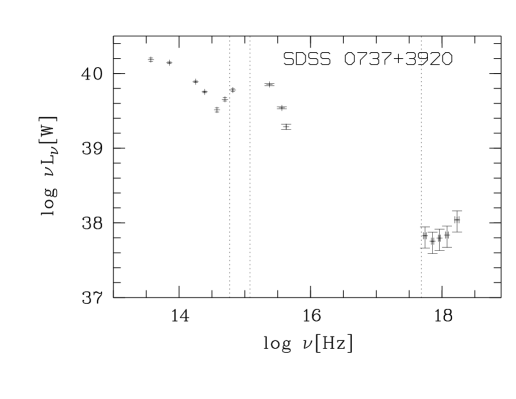
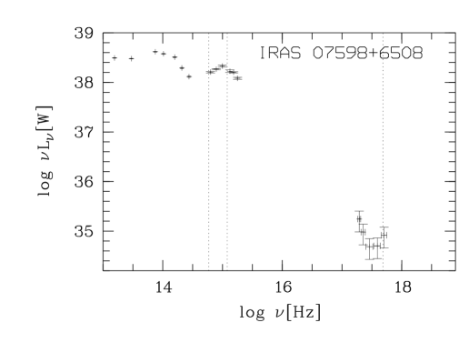
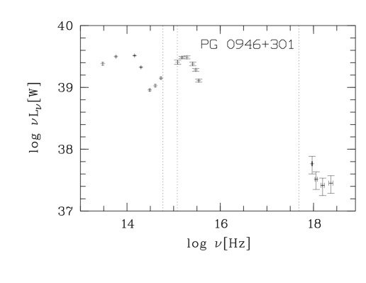
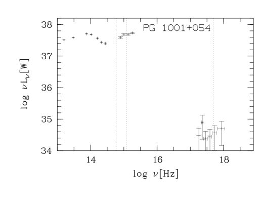
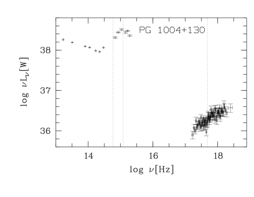
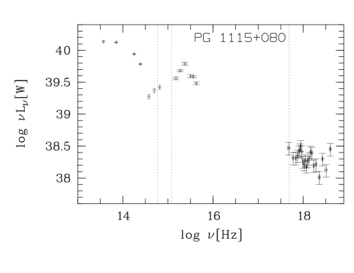
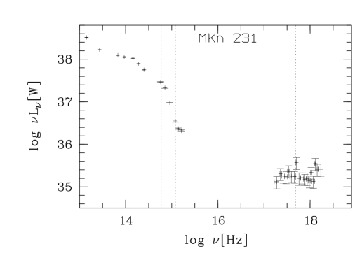
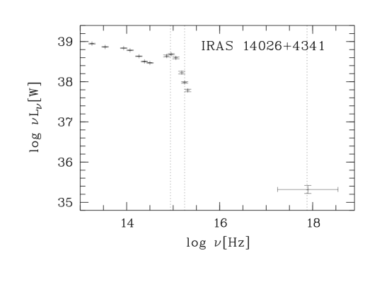
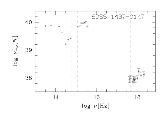
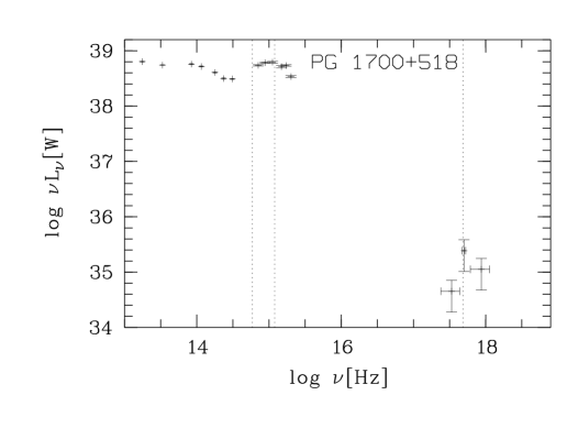
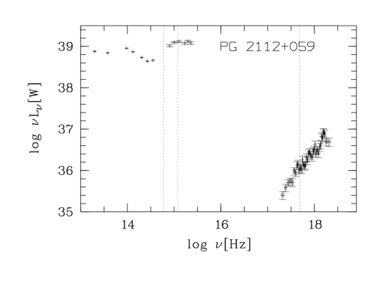
Figure 1: Rest-frame k-corrected IR to X-ray Spectral Energy Distributions of the BAL QSOs. The vertical dashed lines make the rest-frame 5500Å, 2500Å, and 2keV points. Swift  UVOT and XRT data have been corrected for Galactic reddening and absorption.

All Chandra data were fitted initially with an absorbed power law model with the Galactic absorption column density $N_{\rm H}$ listed in Table  1. While this model seems appropriate for most objects, 4 of the sources require an intrinsic absorber at the redshift of the source. While PG 0946+301 can be fitted by a simple neutral absorber, the other three BAL QSOs, PG 1004+130, PG1115+080, and Mkn 231 need be fitted by a partial covering absorber model. The results of all fits to the Chandra data are summarized in Table 4, including the X-ray fluxes in the 0.3-10 keV observed frame. In addition, Table4 also lists the Optical to X-ray spectral slopes $\alpha_{\rm ox}$. These were determined based on the spectral energy distributions using the Chandra and Swift data as shown in Figure 1 (see Section 3.2). Note, however, that the spectral models used here are just a phenomenological description of the spectrum and do not necessarily represent the underlying physics in the source. For example, the geometry of Mkn 231 is highly complex consisting of absorption components as well as contributions from X-ray emission from strong surrounding starburst regions (e.g. Teng et al., 2014, ,and references therein). Nevertheless, our results obtained for PG 1004+130 agree well with those found from the combined Chandra and NuStar data in Luo et al. (2013).

3.2 Spectral Energy Distribution

The spectral energy distributions (SEDs) displayed in Figure 1 were constructed by using the WISE, 2MASS, Swift UVOT, and Chandra X-ray data. All SEDs are shown in rest-frame with k-corrected luminosities. Note that for IRAS 14026+4341 the number of counts detected during the 1.5 ks Chandra observation was too low to obtain a spectral fit. We therefore only give one data point in the 0.3-10 keV regime in the SED which was determined from the count rate during the Chandra observation and converted to flux units assuming a standard AGN spectrum with $\alpha_{\rm X}$=1.0 and Galactic absorption. The bolometric luminosities $L_{\rm bol}$ were measured by integrating over the k-corrected SEDs as shown in Figure 1 between 1$\mu$m and 10 keV (10¹⁴ - $2\times 10^{18}$ Hz). These bolometric luminosities are listed in Table 6. The SEDs were also used to determine $\alpha_{\rm ox}$. These Optical to X-ray spectral slopes are listed in Table 4 together with the expected value estimated from the k-corrected rest-frame luminosity density at 2500Å applying equation (12) in Grupe et al. (2010). Four of the 11 BAL QSOs appear to be clearly X-ray weak following the definition by Brandt et al. (2000) with $\alpha_{\rm ox}$$>$2.0. The $\alpha_{\rm ox}$ criterion for X-ray weakness, however, depends on luminosity. We also determined the difference between the measured $\alpha_{\rm ox}$ and the expected value for the Optical-to-X-ray spectral slope $\alpha_{\rm ox,expected}$ following the relation given in Grupe et al. (2010). As described in Gibson et al. (2009) this parameter is defined as $\Delta$$\alpha_{\rm ox}$ = $\alpha_{\rm ox}$- $\alpha_{\rm ox,expected}$ and for the BAL QSOs in our sample is listed in Table 4.

Although for BAL QSOs absorption is the first thought when a source is detected to be X-ray weak (e.g. Grupe et al., 2003), spectral analysis of the data for these four source does not suggest the presence of a strong absorber. Interestingly, the BAL QSOs in which an intrinsic absorber is clearly detected appear not to be X-ray weak. Alternatively, these sources could be heavily absorbed (i.e. Compton thick), and only a reflected fraction of the intrinsic emission is actually seen. Also, given the quality of the spectral data, a partial covering geometry cannot be excluded. In a partial covering absorber scenario only a fraction of the intrinsic continuum emission is seen directly, while the rest is strongly obscured. Also note again, that some of the BAL QSOs, like PG 1004+130 and PG 1700+518 may be intrinsically X-ray weak (Luo et al., 2013).

3.3 Statistical Analysis

If BAL QSOs and NLS1s represent related phenomena, then some of their characteristic intrinsic properties should be similar. For our study we use the standard definition of NLS1s with a cut off line at FWHM(H$\beta$)=2000 km s^-1.

3.3.1 Distributions

Figure 2 displays the box plots of the distributions of observed and inferred properties of the whole sample (X-ray selected AGN sample of Grupe et al. (2010) plus the Chandra-selected BAL QSOs) on the bottom, NLS1s in the middle and BAL QSOs alone at the top. The mean, standard distribution, and median of these distributions are summarized in Table 7.

While the UV spectral indices of NLS1s and BAL QSOs are very similar, BAL QSOs show significantly flatter X-ray spectral slopes $\alpha_{\rm X}$, and steeper Optical to X-ray spectral slopes $\alpha_{\rm ox}$ than NLS1s. There are several ways to interpret these properties. The flatter X-ray slopes in BAL QSOs may be a consequence of their slightly lower Eddington ratios than NLS1s, as suggested by the relations found by Grupe (2004); Grupe et al. (2010) and Shemmer et al. (2008). They may also imply stronger (cold or ionized) absorption, which was not yet detectable in available X-ray spectra due to short exposure times. The steeper $\alpha_{\rm ox}$ can be primarily explained by stronger absorption in X-rays in BAL QSOs, for example by a partial covering absorber (e.g. Grupe et al., 2003). More importantly, BAL QSOs exhibit much larger $\Delta$$\alpha_{\rm ox}$ parameters than NLS1s.

As for the emission line properties, we noticed that the FWHM([OIII]) of BAL QSOs are significantly larger than those of NLS1s. Note, that these broad NLR emission lines are consistent with BAL QSOs being hosted in significantly larger galaxies. As we will see later, these [OIII] line widths are consistent with the black hole masses measured in BAL QSOs. The [OIII]/H$\beta$ flux ratios in BAL QSOs are significantly lower than compared with NLS1s. The FeII/H$\beta$ ratios of BAL QSOs are larger than those found in NLS1s. This follows the ’eigenvector 1’ relation found by Boroson & Green (1992) in which AGN with stronger FeII emission show weaker emission from the NLR. Compared with the BAL QSO sample of Dietrich et al. (2009), the BAL QSOs in our sample here appear quite extreme in their [OIII]/H$\beta$ and FeII/H$\beta$ line ratios as listed in Table 7. The BAL QSOs in Dietrich et al. (2009) showed mean, standard deviations and medians of –0.63, 0.29, and –0.65, and –0.12, 0.42, and –0.20 for log [OIII]/H$\beta$ and log FeII/H$\beta$, respectively. These values are similar to those found for NLS1s (see Table 7). Note however, that the BAL QSOs in our sample for which optical line ratios could be determined are all at lower redshift, which the BAL QSOs in the Dietrich et al. (2009) sample are all at redshifts around z=2.

BAL QSOs have significantly larger black hole masses than NLS1s. In general, the black hole masses of BAL QSOs are about 100 times larger than those of NLS1s. What is somewhat surprising is that the Eddington ratios $L/L_{\rm Edd}$ of BAL QSOs are about a factor of 10 lower than we found in the NLS1s in our bright soft X-ray selected AGN sample. Figure 7 in Boroson (2002), however, suggested that the Eddington ratios of NLS1s and BAL QSOs are about unity.

Figure 7 in Boroson (2002) also suggests that the mass accretion rates $\dot{M}$ of BAL QSOs and NLS1s are significantly different. As displayed in Figure 2 also when compare our BAL QSO and NLS1 samples we come to a similar conclusion. We estimated the mass accretion rate from the bolometric luminosity with $L_{\rm bol}=\eta\dot{M}c^{2}$ assuming a mass to radiation efficiency of $\eta$=0.1. Also in our sample, BAL QSOs have larger mass accretion rates than NLS1s. Note that some of these mass accretion rates in BAL QSOs exceed 100 $M_{\odot}$/year.

3.3.2 Correlations

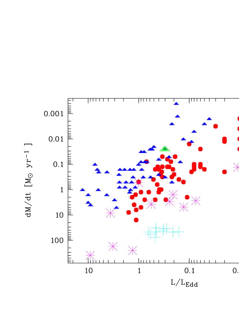
Figure 3: Eddington ratio $L/L_{\rm Edd}$ vs. mass accretion rate $\dot{M}$. BAL QSOs are displayed as large magenta stars, NLS1s as blue solid triangles and BLS1s as red solid circles. WPVS 007 is marked as a large solid green triangle. The cyan crosses mark the BAL QSOs from the sample of Dietrich et al. (2009) as a comparison.

Figure 3 displays the relation between the Eddington ratio $L/L_{\rm Edd}$ and the mass accretion rate $\dot{M}$ following Figure 7 in Boroson (2002). In Figure 3 the BAL QSOs of the Chandra sample are displayed as magenta stars, NLS1s as solid blue triangles, BLS1s as solid red circles, and the BAL QSOs of Dietrich et al. (2009) are shown as turquoise crosses. Clearly, BAL QSOs and NLS1s fall on two separated groups. For a given $L/L_{\rm Edd}$, BAL QSOs have a significantly larger mass accretion rate than NLS1s. This is not completely surprising given the fact that the black hole masses of NLS1s is about a factor of 100 lower than that of BAL QSOs (see also the distributions of black hole masses in Figure 2). However, the plot also shows that the schematic plot shown in Figure 7 in Boroson (2002) is too simple. Although generally speaking, BAL QSOs have higher mass accretion rates than NLS1s, as already shown in Figure 2, there is some overlap between the two groups and the separation between the two classes of AGN is not as strong as suggested in Figure 7 in Boroson (2002). The other difference is that the BAL QSOs in our sample appear to have lower $L/L_{\rm Edd}$ than in the Boroson (2002) sample. The lower $L/L_{\rm Edd}$ found in our BAL QSO sample is similar to those found in the BAL QSOs in Dietrich et al. (2009).

3.3.3 Principal Component Analysis

In order to better understand the relations among the observed parameters we applied a Principal Component Analysis (PCA; Pearson, 1901). to the sample of 119 AGN, including the Swift AGN sample plus the 7 low-redshift BAL QSOs listed in Table 1. A PCA is a standard data mining tool that allows to reduce the number of properties that describe a sample of sources from many to a few. In a mathematical sense, the PCA searches for the eigenvalues and eigenvectors in a correlation coefficient matrix. A good description for the application of a PCA in astronomy can be found in Wills & Francis (1999) and Boroson & Green (1992).

For our sample we used $\alpha_{\rm X}$, $\alpha_{\rm UV}$, $\alpha_{\rm ox}$, $\Delta$$\alpha_{\rm ox}$, FWHM(H$\beta$), FWHM([OIII]), [OIII]/H$\beta$, FeII/H$\beta$ as input parameters in the PCA. The results of the PCA are summarized in Table 8. This PCA is somewhat similar to the one that we applied to basically the same AGN sample in Grupe (2004), although with slightly different input parameters.

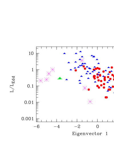
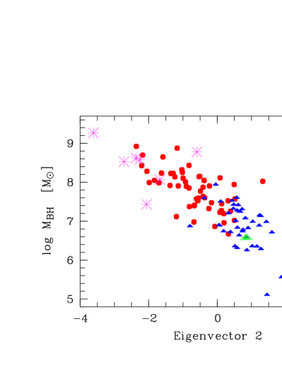
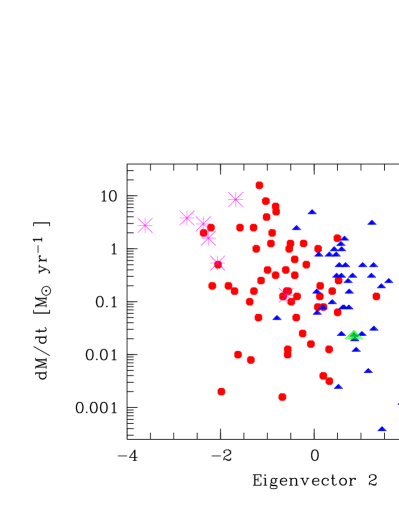
Figure 5: Correlations between Eigenvector 1 and $L/L_{\rm Edd}$, and Eigenvector 2 and black hole mass $M_{\rm BH}$ and the mass accretion rate $\dot{M}$.

Figure 5 displays the correlations between eigenvector 1 and $L/L_{\rm Edd}$, and eigenvector 2 and the black hole mass and $\dot{M}$. While the eigenvector 1 of our sample can be associated with the Eddington ratio $L/L_{\rm Edd}$ (left panel), such as in the PCA performed by Boroson (2002), the eigenvector 2 of our sample is clearly dominated by the black hole mass (middle panel). The Spearman rank order correlation coefficients, Student’s T-test values, and probabilities of a random result of the eigenvector 1 - $L/L_{\rm Edd}$ and eigenvector 2 - $M_{\rm BH}$ correlations are $r_{\rm s}=-0.52$, $T_{\rm s}=-6.62$, $P<10^{-8}$, and $r_{\rm s}=-0.82$, $T_{\rm s}=-15.04$, $P<10^{-8}$, respectively.

Although the mass accretion rate is anti-correlated with eigenvector 2 (right panel) with $r_{\rm s}=-0.32$, $T_{\rm s}=-3.64$, $P=4.1\times 10^{-4}$, it is in our sample also anti-correlated with eigenvector 1 ($r_{\rm s}=-0.44$, $T_{\rm s}=-5.32$, $P=5.2\times 10^{-7}$ However, eigenvectors are orthogonal, which means they should not show a correlation among them. Therefore we conclude that in our sample eigenvector 2 represents the black hole mass and not $\dot{M}$. Note, that for his input sources and input parameters, Boroson (2002) concluded from his PCA that eigenvector 2 represents the mass accretion rate $\dot{M}$. As a test we performed a PCA with just the optical line properties (FWHM(H$\beta$), FWHM([OIII]), [OIII]/H$\beta$, and FeII/H$\beta$). In this case the correlation between eigenvector 2 and $\dot{M}$ becomes more significant with $r_{\rm s}=-0.46$, $T_{\rm s}=-5.67$, $P=1.0\times 10^{-7}$. However, the correlation between eigenvector 2 and the black hole mass is still stronger than that with $\dot{M}$.

4 Discussion

The main motivation behind this study is the question of whether BAL QSOs and NLS1s are intrinsically similar but only appear at different ends of the black hole mass distribution spectrum as suggested by Brandt & Gallagher (2000) and Boroson (2002). Although we see similarities between our sample and that of Boroson (2002), in particular that NLS1s and BLA QSOs have similar FeII/H$\beta$ and [OIII]/H$\beta$ line ratios we also notice differences in the studies.

4.1 Selection Effects

While our sample size is significantly larger than the initial exploratory study of Boroson (2002), it is still subject to selection effects, and we therefore first address the key question, if and how our sample selection affects the parameters we wish to compare among NLS1s and BAL-QSOs:

1. Redshift Distributions: Traditionally, BAL QSOs have been discovered at redshifts of about z=2 (e.g. Weymann et al., 1991). This leads to selecting highly-luminous and therefore high black hole mass AGN. On the other hand, our AGN sample consists of bright X-ray selected AGN which appear at much lower redshifts with z$<$0.4 (Grupe et al., 2004a, 2010). Nevertheless, the 7 low redshift BAL QSOs presented in this paper have redshifts that are between z=0.04 and z=0.47 and fall into the redshift range of our AGN sample. This redshift range is also comparable to the PG sample by Boroson & Green (1992) which contains the BAL QSOs used in Boroson (2002) sample. The 7 low-redhshift BAL QSOs in our sample allow a direct comparison to the low-redshift AGN sample by Grupe et al. (2004a) and Grupe et al. (2010) which is not necessarily true for the high-redshift objects.

2. Soft X-ray selection of the AGN sample: Our AGN sample was selected by their X-ray properties: X-ray bright and soft X-ray spectra (Grupe et al., 1998, 2001, 2004a, 2010). A steep X-ray spectrum, however, is a consequence of high Eddington ratios (Grupe, 2004; Grupe et al., 2010; Shemmer et al., 2008). Therefore the soft X-ray selection favors sources with high L/Ledd among the class of NLS1 galaxies as a whole and the Eddington ratios found in our AGN sample may appear larger than in an optically selected NLS1 sample. The soft X-ray selection also misses highly absorbed AGN, such as typically BAL QSOs.

Although we have to keep these selection effects in mind, they do not make our study invalid. On the contrary, our comparison is between BAL QSOs and NLS1s, and the latter are usually found among soft X-ray selected AGN. It has also been shown that in BAL QSOs and in NLS1s absorbers can develop over time and the absorption column density and covering fraction can vary in X-rays as well as in the UV. For NLS1s a good example here is WPVS 007 which has developed strong BALs within a decade (Leighly et al., 2009). On the other hand, more and more evidence has been found that also the BALs in BAL QSOs can be highly variable (Filiz Ak et al., 2012, 2013; Capellupo et al., 2011, 2012, e.g.).

4.2 Mass accretion rate $\dot{M}$

While Figure 7 in Boroson (2002) suggests that NLS1s and BAL QSOs are both at high $L/L_{\rm Edd}$  where BAL QSOs have significantly larger mass accretion rates than NLS1s, we found from our sample that this picture is more complicated: Although also in our sample BAL QSOs appear to show the highest mass accretion rates, some appear to be significantly lower, even down to 0.1 $M_{\odot}$/year in the case of PG 1004+130. Compared with the BAL QSOs in Dietrich et al. (2009), where the mean mass accretion rate was of the order of about 35 $M_{\odot}$/year, the mass accretion rates in the sample presented here appear to be rather modest with a median of about 4 $M_{\odot}$/year. However, some of the mass accretion rates of the BAL QSOs in our sample are extreme, exceeding 100 $M_{\odot}$/year. The distribution of the mass accretion rates in BAL QSOs spans over three orders of magnitude as shown in Figure 2. Although the mass accretion rate of NLS1s also stretches over three orders of magnitude, the lowest values of the mass accretion rate are of the order of 10^-3 solar masses and the highest of the order of a few solar masses per year. There is a some overlap between NLS1s and BAL QSOs in mass accretion rate in our sample. The two samples are not as separated as the BAL QSO and NLS1s samples of Boroson (2002). This maybe in part a selection effect, because the NLS1s is our sample are soft X-ray selected which are primarily sources with high $L/L_{\rm Edd}$.

If we just focus on the 7 low-redshift BAL QSOs in our study (see Table 1) we notice that the mass accretion rates of these BAL QSOs are in the range between 0.1 to 8 $M_{\odot}$/year and are somewhat comparable to the mass accretion rates seen in NLS1s. The BAL QSOs which really make a difference are those at higher redshifts.

We noticed that the mass accretion rates in BAL QSOs is rather high with more than 100 $M_{\rm sun}$ yr^-1, and 35 in the BAL QSO sample by Dietrich et al. (2009). One reason why these accretion rates appear so high might be our assumption of the mass to radiation efficiency which we for simplicity just set to $\eta=0.1$. If however the black hole spin in BAL QSOs is significantly higher this would increase the efficiency and reduce the mass accretion rate necessary to explain the observed bolometric luminosity. For example, if the black hole in a BAL QSO is maximal spinning (a=0.998) the efficiency will be $\eta=0.32$, or three times higher than our assumed $\eta$=0.1. This would imply that the mass accretion rate is a factor of 3 lower, which is much easier to explain than the high mass accretion rates we estimated at first. In contrast to BAL QSOs, in NLS1s the efficiency may be lower and the mass accretion rate higher if the black hole is rotating slower than in our assumption. Keep in mind that for an efficiency of $\eta=0.1$ the black hole is spinning already with a=0.6. One argument that the black hole spins in BAL QSOs and NLS1s are systematically different, is the finding that the black hole masses in BAL QSOs are significantly larger than in NLS1s. A larger black hole mass also means that the accreted matter has transferred a larger amount of angular momentum to this black hole which then results in a larger spin (in a scenario where SMBHs primarily grow by accretion). One more argument for a higher efficiency of the mass to radiation conversion due to a relativistically spinning black hole is that the mass accretion rates in the sample presented here appear to be relatively low compared with those of the BAL QSO sample by Dietrich et al. (2009).

4.3 Eddington ratios $L/L_{\rm Edd}$

The BAL QSOs in our sample also have Eddington ratios $L/L_{\rm Edd}$ which are lower than those of NLS1s. In Figure 7 in Boroson (2002) shows that the BAL QSOs in the Boroson & Green (1992) sample are all at $L/L_{\rm Edd}$=1, which is typical for NLS1s. Although our AGN/NLS1 sample is soft X-ray selected and has therefore a bias towards high $L/L_{\rm Edd}$ AGN, the Eddington ratios found in our sample agree well with those of the NLS1s in the optically selected sample by Boroson & Green (1992). However, a comparison between our sample and that of Boroson (2002) appears somewhat difficult because Boroson & Green (1992) do not list the values of $L/L_{\rm Edd}$ and $\dot{M}$ of the NLS1s and BAL QSOs of their PG quasar sample.

Although the eigenvector 1 in our PCA can also be associated with the Eddington ratio $L/L_{\rm Edd}$ as in the Boroson (2002) sample, our eigenvector 2 seems to be different. While Boroson (2002) suggested that the eigenvector 2 in his sample is clearly associated with the mass accretion rate $\dot{M}$, in our sample eigenvector 2 is more strongly correlated with the black hole mass. These differences are not surprising. A PCA is a purely mathematical tool and the results depend strongly on the set of input parameters as well as the objects in the sample. While in our PCA we used continuum properties and line widths and ratios, the PCA in Boroson (2002) primarily used optical line properties. Therefore it can be expected that the results of the PCAs could be different. However, when we only use optical line parameters in a PCA, we still find that in our sample that eigenvector 2 is strongly correlated with the black hole mass.

4.4 Black Hole Masses and Growth

From our BAL QSO and NLS1 samples we found that BAL QSOs have black hole masses more than 100 times larger than those seen in a typical NLS1. At first glance this seems to be a selection effect because most BAL QSOs appear at higher redshifts which leads to selecting objects with higher luminosities and larger back hole masses. However, for low-redshift BAL QSOs in our Chandra sample, we note that even these objects have black hole masses of the order of $10^{9}$$M_{\odot}$, significantly larger than those found in NLS1s (see Figure 2).

In contrast to NLS1s, BAL QSOs may have already fully developed black holes with regards to their host galaxy masses. This argument is supported by the M - $\sigma$ relation which relates the mass of the central black hole to that of the host galaxy. BAL QSOs fall right on the Tremaine et al. (2002) M - $\sigma$ relation as shown in in Figure 6 (the Tremaine et al. (2002) relation is shown as a black solid line), while NLS1s typically fall below this relation (Grupe & Mathur, 2004). We adopted the method introduced by Nelson (2000) who suggested to use the [OIII] line as a proxy of the stellar velocity dispersion in the host galaxy bulge. Because the Narrow Line Region is in the gravitational potential of the host galaxy bulge, the NLR gas follows the same velocity dispersion as the bulge stars. As a comparison we also show the BAL QSOs from the study by Dietrich et al. (2009) in this plot. Note that the BAL QSO of the Dietrich et al. (2009) sample have redshifts between z=1-2 and from our BAL QSO sample we have only [OIII] and H$\beta$ measurements of the 7 low-redshift BAL QSOs. The BAL QSOs of our sample which are at higher redshifts also have similar black hole masses as the objects in the Dietrich et al. (2009) BAL QSO sample. Whether NLS1 galaxies, as a group, fall on or below the $M-\sigma_{\rm[OIII]}$ relation is an important question (e.g. Grupe & Mathur, 2004; Mathur & Grupe, 2005a, b; Komossa & Xu, 2007) The only BAL QSO that falls below the M - $\sigma_{\rm[OIII]}$ relation is PG 1001+054. The (soft X-ray selected) NLS1 sample of Grupe & Mathur (2004) was located significantly below the $M-\sigma_{\rm[OIII]}$ relation, while the NLS1 sample of Komossa & Xu (2007) was consistent with the $M-\sigma_{\rm[OIII]}$ relation of non-active galaxies, with the exception of sources at high $L/L_{\rm Edd}$. These had their whole [OIII] emission systematically blueshifted (“blue outliers”), implying large outflows which come with a strong extra line broadening apparently displacing them from the $M-\sigma_{\rm[OIII]}$ relation. Therefore the FWHM([OIII]) measured in these objects may not represent the velocity of the velocity dispersion in the bulge, but has an additional, unknown contribution by outflows. In the same way as turbulent motion can lead to an overestimation of the the black hole masses from BLR emission line widths as shown by Kollatschny & Zetzl (2011), an outflow adds an additional velocity component to the total velocity and therefore leads to an overestimation of the mass of the host galaxy bulge.

4.5 Outflows in BAL QSOs and NLS1s

The main question remaining is why do we see strong outflows which appear as deep UV absorption troughs in BAL QSOs but these are rarely seen in NLS1s. In a matter of fact, the only NLS1s that has shown dramatic UV absorption roughs is WPVS 007. Part of the answer maybe that BAL QSOs are highly-luminous AGN and as shown by Laor & Brandt (2002), the strengths of the BAL troughs correlates with luminosity. Nevertheless, the NLS1 WPVS 007 is a low luminosity AGN and seems to contradict these findings. Strong outflows are typically associated with high $L/L_{\rm Edd}$ which results in a strong radiation field from the accretion disk producing radiation driven winds/outflows Proga & Kallman (e.g. 2004); Kurasawa & Proga (e.g. 2009a, b). On the other hand, NLS1s with high $L/L_{\rm Edd}$ exhibit strong outflows through their broad, blueshifted [OIII] emission lines (e.g. Bian et al., 2005; Zhang et al., 2011; Xu et al., 2012), which we do not see in BAL QSOs (e.g. Dietrich et al., 2009).

4.6 Overall Comparison and Conclusions

One reason for the slight differences between our study and that by Boroson (2002) maybe the different sample sizes. While in our sample we have 11 BAL QSOs (7 at low redshift) and 53 NLS1s, the numbers in the Boroson (2002) sample are 4 BAL QSOs and 8 NLS1s. The low number of in particular BAL QSOs may have a large influence on these differences. As mentioned about, the mass accretion rates in other BAL QSO samples, like that in Dietrich et al. (2009) appear to be larger. Therefore in a sample of just 4 sources, the chance of selecting BAL QSOs with larger mass accretion rates is quite high.

To conclude, we confirm the results by Brandt & Gallagher (2000) and Boroson (2002) about the differences in the black hole mass distributions between BAL QSOs and NLS1s. We also confirm that the Eddington ratios of BAL QSOs and NLS1s are at the higher end of the $L/L_{\rm Edd}$ distribution of AGN in general. However, from our samples of NLS1s and BAL QSOs the Eddington ratios NLS1s typically operate around unity, while those of the BAL QSOs are slightly lower. NLS1s and BAL QSO also share that their FeII/H$\beta$ ratios are very high and their [OIII]/H$\beta$ ratios are low - following the ’classic Boroson & Green (1992)’ eigenvector 1 relation. Although some BAL QSOs in our sample exhibit very high mass accretion rates inferred from their bolometric luminosities, the mass accretion rates of BAL QSOs and NLS1s appear to be more similar than previously thought. This is in particular true when we look at the low redshift BAL QSOs in our sample. Interestingly, even though BAL QSOs have relatively large $L/L_{\rm Edd}$ ratios, they fall right onto the $M_{\rm BH}-\sigma_{\rm[OIII]}$ relation suggesting that they have fully developed black holes. One reason for the large bolometric luminosities found in BAL QSOs may be that the black hole is spinning relativistically which leads to a significantly higher efficiency of the mass to radiation conversion. In the future we need to increase the number of BAL QSOs in our study to obtain better statistics on the relations found in our study. In particular we need to obtain more X-ray observations of BAL QSOs to measure the continuum properties. And last but not least, in the far future we need to study the Fe K$\alpha$ line emission line to study the gravitational and relativistic effects which can be used to measure the black hole spin.

Figure 2: Box plots of the distributions of the whole AGN (X-ray selected sample by Grupe et al. (2010) and BAL QSOs) at the bottom, ’classical’ NLS1s in the middle, and BAL QSOs alone at the top.

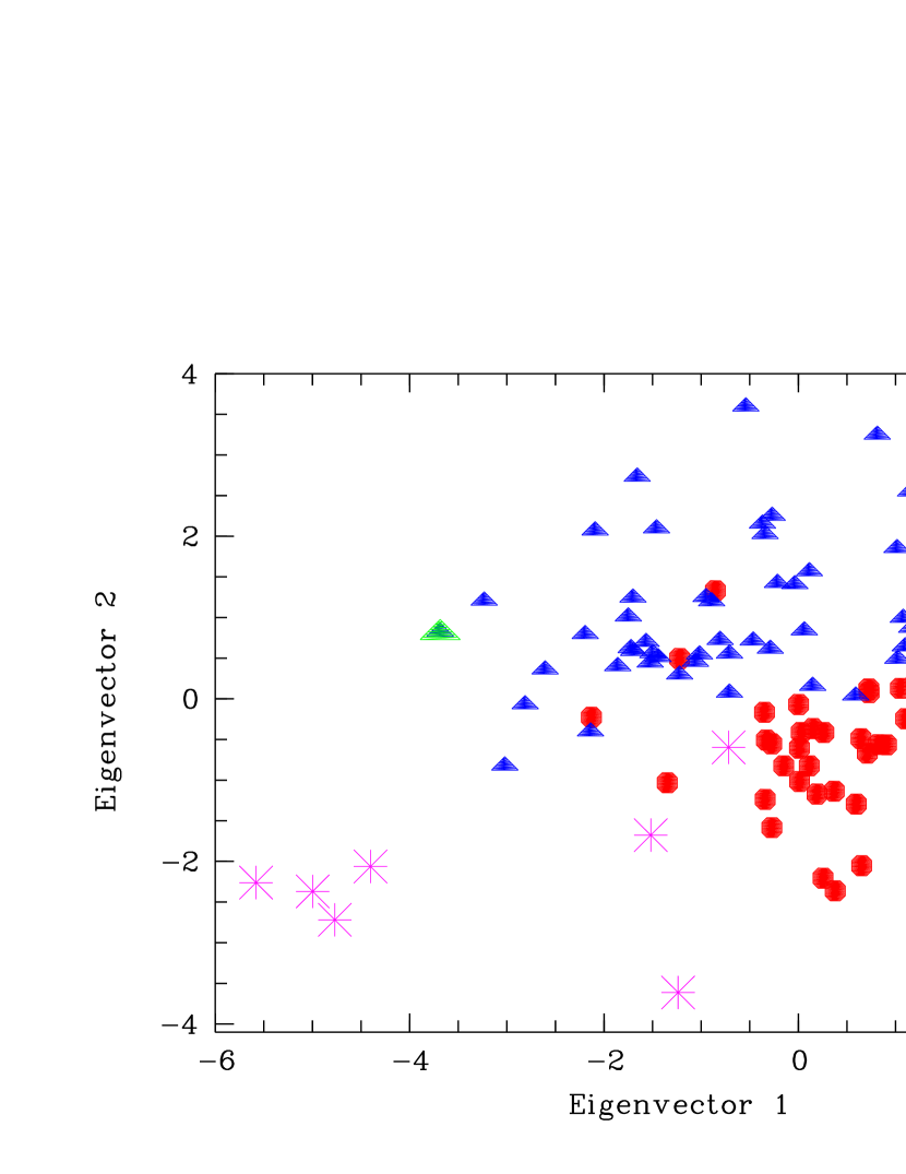
Figure 4: Eigenvector 1 vs. Eigenvector 2 diagram. The symbols are the same as defined in Figure 3.

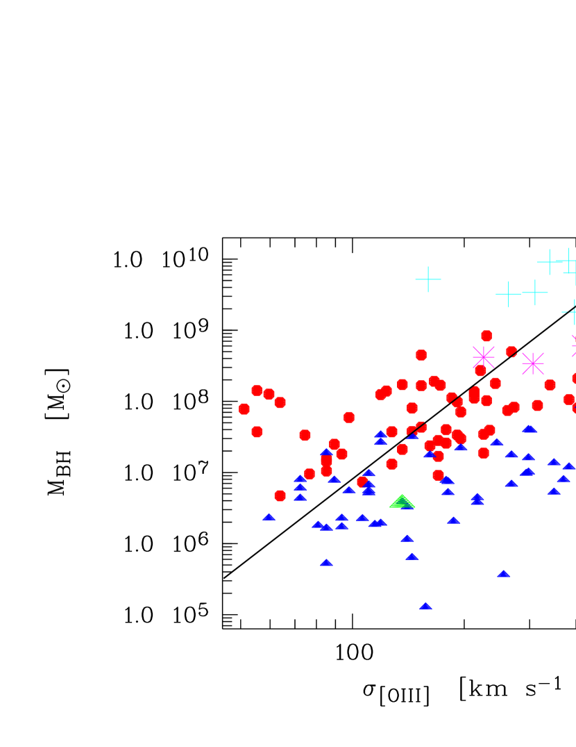
Figure 6: M - $\sigma$ relation for the AGN and BAL QSOs in the sample. The symbols are the same as defined in Figure 3. The cyan crosses mark the BAL QSOs from the sample of Dietrich et al. (2009) as a comparison.

Table 1: Object summary and chandra  Observation log of the BAL QSOs

Object Name	RA-2000	Dec-2000	z	$D_{\rm L}$	$N_{\rm H,gal}$	EB-V	TargetID	T-start	T-stop	MJD	$T_{\rm exp}$
SDSS J073733+392037	07 37 33.0	+39 20 37.4	1.7360	12499.4	5.84	0.046	13346	2011-11-14 07:54	2011-11-14 08:54	55879.3500	1539
IRAS 07598+6508	08 04 33.1	+64 59 49.0	0.1483	659.6	4.17	0.047	11850	2010-06-18 08:11	2010-06-18 10:53	55365.3958	6684
PG 0946+301	09 49 41.1	+29 55 19.0	1.2235	8081.1	1.71	0.016	11854	2010-01-11 08:09	2010-01-11 10:30	55207.3889	6518
PG 1001+054	10 04 20.1	+05 13 00.5	0.1611	722.4	1.83	0.014	11852	2010-01-11 06:23	2010-01-11 08:09	55207.3021	1597
PG 1004+130	10 07 26.1	+12 48 56.1	0.2406	1132.1	3.56	0.034	05606	2005-01-05 16:55	2005-01-06 04:37	53375.9479	41064
PG 1115+080	11 18 16.9	+07 45 58.2	1.7355	12494.9	3.57	0.036	11857	2010-02-01 01:57	2010-02-01 06:40	55228.1806	14582
Mkn 231	12 56 14.2	+56 52 25.2	0.0422	174.3	0.96	0.008	11851	2010-07-11 01:51	2010-07-11 03:52	55388.1188	4782
IRAS 14026+4341	14 04 38.8	+43 27 07.4	0.3233	1591.4	1.15	0.010	11855	2010-07-28 14:41	2010-07-28 16:56	55405.6583	6684
SDSS 1437-0147	14 37 48.3	-01 47 10.7	1.311	8809.6	3.21	0.039	11851	2010-07-11 01:51	2010-07-11 03:52	55388.1194	4782
PG 1700+518	17 01 24.8	+51 49 20.0	0.2920	1413.8	2.26	0.030	11853	2010-06-26 19:51	2010-06-26 22:26	55373.8819	6684
PG 2112+059	21 14 52.6	+06 07 42.5	0.466	2454.5	6.09	0.080	03011	2002-09-01 06:35	2002-09-01 23:45	52518.6528	56868

Table 2: Swift  Observation log of the BAL QSOs

Object Name	ObsID	Segment	T-start	T-stop	MJD	$\rm T_{\rm XRT}$	$\rm T_{\rm V}$	$\rm T_{\rm B}$	$\rm T_{\rm U}$	$\rm T_{\rm UVW1}$	$\rm T_{\rm UVM2}$	$\rm T_{\rm UVW2}$
SDSS J073733+392037	39544	001	2011-08-29 09:41	2011-08-22 22:39	55795.6319	3311	$\cdots$	$\cdots$	$\cdots$	$\cdots$	3294	$\cdots$
		002	2012-01-15 03:45	2012-01-15 03:50	55941.1576	235	$\cdots$	$\cdots$	$\cdots$	$\cdots$	$\cdots$	254
		003	2012-03-22 05:10	2012-03-22 05:20	56008.2188	584	$\cdots$	$\cdots$	582	$\cdots$	$\cdots$	$\cdots$
IRAS 07598+6508	80519	001	2013-10-29 21:07	2013-10-29 23:01	56594.9132	2093	84	84	81	169	1296	338
PG 0946+301	08523	001	2013-11-09 23:05	2013-11-09 23:32	56605.9708	1606	131	131	131	261	397	522
		002	2013-11-10 00:41	2013-11-10 00:58	56606.0347	1014	85	85	85	171	227	342
PG 1001+054	80521	001	2013-06-28 08:26	2013-06-28 10:22	56471.3889	1591	$\cdots$	95	95	1256	$\cdots$	247
PG 1004+130	80031	001	2012-10-29 08:12	2012-10-29 10:04	56229.3805	1975	$\cdots$	$\cdots$	$\cdots$	$\cdots$	$\cdots$	1966
	33077	001	2014-01-10 00:36	2014-01-10 08:34	56667.1910	1838	156	156	156	312	442	626
PG 1115+080	90073	008	2010-02-19 10:19	2010-02-20 15:42	55247.0729	18832	$\cdots$	$\cdots$	$\cdots$	1650	$\cdots$	1305
		010	2010-03-26 02:32	2010-03-26 23:36	55281.5431	19102	$\cdots$	$\cdots$	$\cdots$	1569	$\cdots$	1335
	33106	001	2014-01-17 16:30	2014-01-14 18:22	56674.7257	2168	179	179	179	358	487	718
Mkn 231	32530	001	2012-08-26 04:45	2012-08-26 11:29	56165.3368	2303	$\cdots$	$\cdots$	$\cdots$	$\cdots$	$\cdots$	2291
	80091	001	2013-05-09 13:02	2013-05-09 13:21	56421.5500	1124	$\cdots$	$\cdots$	$\cdots$	$\cdots$	$\cdots$	1121
	32530	002	2014-01-10 19:53	2014-01-10 21:43	56667.8667	2437	202	202	202	404	556	810
IRAS 14026+4341	80520	001	2013-11-10 21:54	2013-11-10 23:43	56606.9493	1868	87	87	87	175	1072	351
SDSS 1437-0147	91050	001	2012-03-08 09:14	2012-03-08 12:28	55994.4521	250	$\cdots$	$\cdots$	$\cdots$	$\cdots$	251	$\cdots$
		002	2012-03-08 09:16	2012-03-08 12:37	55994.4556	1481	$\cdots$	$\cdots$	$\cdots$	284	$\cdots$	$\cdots$
	33097	002	2014-01-18 12:22	2014-01-18 14:06	56675.5521	1029	35	158	158	315	103	215
		003	2014-01-22 12:14	2014-01-22 12:31	56679.5153	1006	83	83	84	168	231	336
PG 1700+518	37605	001	2008-07-06 12:19	2008-07-07 20:35	54654.1875	7364	626	626	626	1253	1603	2506
		002	2008-07-08 02:28	2008-07-08 09:14	54655.2438	2892	347	347	347	694	622	1389
	80179	001	2012-09-22 21:18	2012-09-22 21:36	56192.8916	1064	$\cdots$	$\cdots$	1063	$\cdots$	$\cdots$	$\cdots$
PG 2112+059	33320	001	2014-06-19 14:31	2014-06-19 19:25	56827.7069	1284	$\cdots$	$\cdots$	120	1140	$\cdots$	$\cdots$
		002	2014-06-21 00:24	2014-06-21 00:30	56829.0188	331	$\cdots$	$\cdots$	$\cdots$	$\cdots$	$\cdots$	326
		003	2014-06-25 04:55	2014-06-25 21:20	56833.5472	1638	$\cdots$	$\cdots$	$\cdots$	$\cdots$	$\cdots$	1634
		004	2014-07-01 14:44	2014-07-01 16:28	55379.6493	747	$\cdots$	$\cdots$	$\cdots$	735	$\cdots$	$\cdots$
		005	2014-07-03 07:48	2014-07-03 07:58	56841.3285	587	48	48	48	97	130	194
		006	2014-07-08 22:34	2014-07-08 22:37	56846.9410	152	$\cdots$	19	43	85	$\cdots$	$\cdots$

Table 3: 2MASS and WISE fluxes

	2MASS			WISE
Object Name	J	H	K	W1	W2	W3	W4
SDSS J073733+392037	0.319$\pm$0.012	0.240$\pm$0.013	0.173$\pm$0.011	0.176$\pm$0.004	0.241$\pm$0.005	0.433$\pm$0.010	0.476$\pm$0.024
IRAS 07598+6508	2.496$\pm$0.075	3.731$\pm$0.094	6.182$\pm$0.109	7.378$\pm$0.158	8.086$\pm$0.143	5.873$\pm$0.076	6.071$\pm$0.090
PG 0946+301	0.341$\pm$0.013	0.257$\pm$0.012	0.219$\pm$0.009	0.265$\pm$0.006	0.410$\pm$0.008	0.394$\pm$0.010	0.302$\pm$0.016
PG 1001+054	0.362$\pm$0.017	0.393$\pm$0.014	0.527$\pm$0.016	0.807$\pm$0.017	0.837$\pm$0.016	0.633$\pm$0.012	0.540$\pm$0.021
PG 1004+130	0.806$\pm$0.023	0.635$\pm$0.025	0.673$\pm$0.020	0.715$\pm$0.015	0.765$\pm$0.014	0.955$\pm$0.016	1.121$\pm$0.038
PG 1115+080	0.259$\pm$0.017	0.231$\pm$0.017	0.185$\pm$0.013	0.213$\pm$0.005	0.305$\pm$0.006	0.464$\pm$0.010	0.478$\pm$0.019
Mkn 231	14.880$\pm$0.280	20.566$\pm$0.346	27.600$\pm$0.433	30.110$\pm$0.872	33.400$\pm$0.747	44.961$\pm$0.416	87.351$\pm$0.895
IRAS 14026+4341	0.799$\pm$0.018	0.865$\pm$0.023	1.169$\pm$0.021	1.896$\pm$0.041	2.149$\pm$0.040	2.295$\pm$0.034	2.778$\pm$0.057
SDSS 1437-0147	0.571$\pm$0.017	0.519$\pm$0.019	0.356$\pm$0.013	0.393$\pm$0.008	0.635$\pm$0.012	0.697$\pm$0.012	0.657$\pm$0.021
PG 1700+518	1.140$\pm$0.024	1.159$\pm$0.035	1.490$\pm$0.027	2.124$\pm$0.044	2.341$\pm$0.041	2.249$\pm$0.027	2.592$\pm$0.046
PG 2112+059	0.571$\pm$0.019	0.543$\pm$0.016	0.666$\pm$0.019	1.034$\pm$0.022	1.268$\pm$0.024	0.976$\pm$0.015	1.063$\pm$0.031

Table 4: Analysis of the Chandra data

Object Name	MJD	Model	$\alpha_{\rm X}$	$N_{\rm H,z}$	$f_{\rm pc}$	$F_{\rm 0.3-10keV}$	$\alpha_{\rm ox}$	$\alpha_{\rm ox,expected}$	$\Delta$$\alpha_{\rm ox}$
SDSS J073733+392037	55879.3500	powl	0.80${}^{+0.42}_{-0.41}$	—	—	4.33$\pm$0.80	1.80$\pm$0.07	1.66	+0.14
IRAS 07598+6508	55365.3958	powl	1.37${}^{+0.91}_{-0.68}$	—	—	4.45$\pm$1.21	2.34$\pm$0.10	1.47	+0.87
PG 0946+301	55207.3889	zwa	1.09${}^{+0.98}_{-0.86}$	13.06${}^{+9.15}_{-6.96}$	—	3.15$\pm$0.25	1.63$\pm$0.35	1.59	+0.04
PG 1001+054	55207.3021	powl	0.86${}^{+1.03}_{-0.99}$	—	—	0.24$\pm$0.13	2.20$\pm$0.17	1.40	+0.80
PG 1004+130	53375.9479	zpcfabs	0.50$\pm$0.21	1.15${}^{+0.66}_{-0.72}$	0.64${}^{+0.10}_{-0.14}$	6.63$\pm$0.15	1.86$\pm$0.06	1.49	+0.37
PG 1115+080	55228.1806	zpcfabs	1.35${}^{+0.40}_{-0.38}$	10.65${}^{+4.57}_{-4.16}$	0.92${}^{+0.05}_{-0.06}$	7.27$\pm$0.50	1.42$\pm$0.10	1.61	–0.19
Mkn 231	55388.1188	zpcfabs	1.00 (fix)	4.75${}^{+3.23}_{-1.68}$	0.90${}^{+0.03}_{-0.04}$	17.23$\pm$1.84	1.49$\pm$0.06	1.26	+0.23
IRAS 14026+4341	55405.6583	powl	1.00 (fix)	—	—	0.06${}^{+0.03}_{-0.02}$	2.23$\pm$0.37	1.50	+0.73
SDSS 1437-0147	55388.1194	powl	0.68${}^{+0.32}_{-0.30}$	—	—	12.11$\pm$0.17	1.72$\pm$0.07	1.65	+0.07
PG 1700+518	55373.8819	powl	0.89${}^{+1.10}_{-0.92}$	—	—	0.15$\pm$0.01	2.42$\pm$0.12	1.52	+0.90
PG 2112+059	52518.6528	zpcfabs	0.75$\pm$0.32	5.83${}^{+1.75}_{-1.62}$	0.82${}^{+0.08}_{-0.13}$	2.04$\pm$0.10	1.78$\pm$0.05	1.57	+0.21

Table 5: Fluxes of the BAL QSOs from the Swift observations

Object Name	ObsID	Segment	MJD	$\rm F_{\rm 0.3-10keV}$	$\rm F_{\rm V}$	$\rm F_{\rm B}$	$\rm F_{\rm U}$	$\rm F_{\rm UVW1}$	$\rm F_{\rm UVM2}$	$\rm F_{\rm UVW2}$	$\alpha_{\rm UV}$	$\rm l_{\rm 2500\AA}$
SDSS J073733+392037	39544	001	55795.6319	3.11$\pm$0.72	$\cdots$	$\cdots$	$\cdots$	$\cdots$	0.45$\pm$0.02	$\cdots$
		002	55941.1576		$\cdots$	$\cdots$	$\cdots$	$\cdots$	$\cdots$	0.26$\pm$0.02	—	7.24
		003	56008.2188	5.63$\pm$1.35	$\cdots$	$\cdots$	0.94$\pm$0.04	$\cdots$	$\cdots$	$\cdots$
IRAS 07598+6508	80519	001	56594.9132	$<$1.03	3.35$\pm$0.13	3.84$\pm$0.12	4.43$\pm$0.22	3.49$\pm$0.20	3.31$\pm$0.10	2.51$\pm$0.12	0.39$\pm$0.01	0.154
PG 0946+301	08523	001	56605.9708		0.45$\pm$0.04	0.53$\pm$0.02	0.53$\pm$0.03	0.42$\pm$0.03	0.33$\pm$0.02	0.22$\pm$0.01
		002	56606.0347	1.9${}^{+1.9}_{-1.0}$	0.49$\pm$0.04	0.58$\pm$0.03	0.50$\pm$0.03	0.40$\pm$0.03	0.35$\pm$0.02	0.22$\pm$0.02	0.61$\pm$0.22	1.95
PG 1001+054	80521	001	56471.3889	$<$2.24	$\cdots$	0.66$\pm$0.04	0.82$\pm$0.05	0.82$\pm$0.04	$\cdots$	0.91$\pm$0.05	0.65$\pm$0.12	0.040
PG 1004+130	80031	001	56229.3805	1.91${}^{+0.95}_{-0.71}$	$\cdots$	$\cdots$	$\cdots$	$\cdots$	$\cdots$	1.47$\pm$0.06
	33077	001	56667.1910	2.41${}^{+1.09}_{-0.48}$	1.43$\pm$0.06	1.92$\pm$0.06	2.25$\pm$0.09	1.90$\pm$0.11	2.08$\pm$0.07	1.58$\pm$0.07	0.68$\pm$0.20	0.245
PG 1115+080	90073	008	55247.0729	3.70$\pm$0.61	$\cdots$	$\cdots$	$\cdots$	0.91$\pm$0.05	$\cdots$	0.64$\pm$0.03
		010	55281.5431	4.17$\pm$0.58	$\cdots$	$\cdots$	$\cdots$	0.90$\pm$0.05	$\cdots$	0.64$\pm$0.03
	33106	001	56674.7257	5.83$\pm$1.01	0.62$\pm$0.03	0.81$\pm$0.03	1.04$\pm$0.05	0.66$\pm$0.04		0.51$\pm$0.03	$-$0.15$\pm$0.06	2.63
Mkn 231	32530	001	56165.3368	8.60$\pm$2.13	$\cdots$	$\cdots$	$\cdots$	$\cdots$	$\cdots$	0.57$\pm$0.03
	80091	001	56421.5500	6.85${}^{+2.70}_{-2.23}$	$\cdots$	$\cdots$	$\cdots$	$\cdots$	$\cdots$	0.50$\pm$0.02
	32530	002	56667.8667	1.70$\pm$0.42	7.17$\pm$0.17	5.26$\pm$0.10	2.32$\pm$0.09	0.87$\pm$0.08	0.57$\pm$0.02	0.51$\pm$0.03	3.80$\pm$0.19	2.4$\times 10^{-3}$
IRAS 14026+4341	80520	001	56606.9493	$<$0.98	1.34$\pm$0.07	1.47$\pm$0.06	1.20$\pm$0.06	0.52$\pm$0.04	0.29$\pm$0.01	0.19$\pm$0.01	1.25$\pm$0.36	0.309
SDSS 1437-0147	91050	001	55994.4521		$\cdots$	$\cdots$	$\cdots$	$\cdots$	1.74$\pm$0.07	$\cdots$
		002	55994.4556	10.48${}^{+6.73}_{-2.42}$	$\cdots$	$\cdots$	$\cdots$	1.84$\pm$0.10	$\cdots$	$\cdots$
	33097	002	56675.5521		1.03$\pm$0.10	1.23$\pm$0.05	1.53$\pm$0.07	1.59$\pm$0.09	1.74$\pm$0.09	1.15$\pm$0.07	0.43$\pm$0.09	5.01
		003	56679.5153	16.21${}^{+4.45}_{-2.60}$	1.18$\pm$0.07	1.40$\pm$0.06	1.66$\pm$0.08	1.67$\pm$0.10	1.58$\pm$0.07	1.16$\pm$0.06	0.53$\pm$0.14
PG 1700+518	37605	001	54654.1875	0.45${}^{+0.18}_{-0.14}$	2.22$\pm$0.06	2.48$\pm$0.06	2.54$\pm$0.06	2.11$\pm$0.07	2.21$\pm$0.08	1.40$\pm$0.06	1.08$\pm$0.12
		002	54655.2438	$<$0.75	2.13$\pm$0.06	2.45$\pm$0.06	2.40$\pm$0.09	1.75$\pm$0.06	2.21$\pm$0.07	1.17$\pm$0.05	0.457
	80179	001	56192.8916	$<$2.01	$\cdots$	$\cdots$	2.73$\pm$0.11	$\cdots$	$\cdots$	$\cdots$
PG 2112+059	33320	001	56827.7069	$2.7^{+1.5}_{-1.2}$	$\cdots$	$\cdots$	1.87$\pm$0.09	1.88$\pm$0.10	$\cdots$	$\cdots$	$\cdots$	0.07
		002	56829.0188	$<$19.2	$\cdots$	$\cdots$	$\cdots$	$\cdots$	$\cdots$	2.04$\pm$0.10	$\cdots$
		003	56833.5472	$<$3.0	$\cdots$	$\cdots$	$\cdots$	$\cdots$	$\cdots$	2.00$\pm$0.09	$\cdots$
		004	55379.6493	$<$6.4	$\cdots$	$\cdots$	$\cdots$	1.90$\pm$0.10	$\cdots$	$\cdots$	$\cdots$	0.08
		005	56841.3285	$<$15.7	1.49$\pm$0.10	1.81$\pm$0.08	1.88$\pm$0.11	1.70$\pm$0.12	1.92$\pm$0.11	1.73$\pm$0.13	0.89$\pm$0.10	0.08
		006	56846.9410	$\cdots$	$\cdots$	1.97$\pm$0.12	2.04$\pm$0.11	1.85$\pm$0.13	$\cdots$	$\cdots$	$\cdots$	0.06

Table 6: Black hole masses and $L/L_{\rm Edd}$

Object Name	FW(H$\beta$)	FW(MgII)	log $L_{\rm 5100\AA}$	log $L_{\rm 3000\AA}$	log $M_{\rm BH}$	log $L_{\rm Edd}$	log $L_{\rm bol}$	log $L/L_{\rm Edd}$	FW([OIII])	log([OIII]/H$\beta$)	log(FeII/H$\beta$)
SDSS J073733+392037	—	8470	—	2.51	9.98	4.07	4.20	+0.12	—	—	—
IRAS 07598+6508	3400	—	1.20	—	8.58	2.68	2.00	–0.68	1050	–1.31	+0.42
PG 0946+301	—	4180	—	2.35	9.28	3.38	2.49	–0.89	—	—	—
PG 1001+054	1500	—	0.54	—	7.43	1.53	1.53	+0.00	1200	–0.94	–0.03
PG 1004+130	8300	—	1.25	—	9.27	3.37	2.24	–1.13	1100	–0.63	–0.42
PG 1115+080	—	4215	—	2.40	9.31	3.41	4.39	+0.96	—	—	—
Mkn 231	6530	—	0.47	—	8.78	2.88	0.92	–1.96	980	–0.93	+0.32
IRAS 14026+4341	2880	—	1.58	—	8.62	2.72	2.27	–0.61	530	–2.35	+0.28
SDSS 1437-0147	—	4770	—	2.42	9.43	3.53	4.04	+0.51	—	—	—
PG 1700+518	2440	—	1.69	—	8.53	2.63	2.38	–0.25	720	–1.23	–0.01
PG 2112+059	3010	—	1.48	—	8.07	2.17	2.73	+0.56	1200	–0.56	–0.09

Table 7: Mean, standard deviation, and median of whole AGN sample including BAL QSOs, NLS1s and BAL QSOs

	All AGN				NLS1s				BAL QSOs
Property	Mean	SD	Median	# of AGN	Mean	SD	Median	# of NLS1s	Mean	SD	Median	# of BAL QSOs
$\alpha_{\rm X}$	1.327	0.509	1.250	123	1.661	0.470	1.590	54	0.936	0.266	0.890	11
$\alpha_{\rm UV}$	0.869	0.772	0.690	122	0.878	0.762	0.690	54	0.963	1.070	0.665	10
$\alpha_{\rm ox}$	1.385	0.247	1.340	123	1.386	0.228	1.400	54	1.899	0.345	1.800	11
$\Delta$$\alpha_{\rm ox}$	0.031	0.211	0.009	119	0.059	0.201	0.009	52	0.379	0.381	0.230	11
log FWHM(H$\beta$)	3.365	0.263	3.382	119	3.124	0.120	3.161	54	3.539	0.253	3.491	7
log FWHM([OIII])	2.608	0.259	2.607	119	2.610	0.264	2.574	54	2.971	0.132	3.021	7
log [OIII]/H$\beta$	–0.439	0.513	–0.482	119	–0.507	0.498	–0.569	54	–1.136	0.603	–0.940	7
log FeII/H$\beta$	–0.178	0.323	–0.161	119	–0.001	0.264	–0.023	54	+0.067	0.292	–0.010	7
log $M_{\rm BH}$	7.458	0.846	7.430	123	6.805	0.559	6.844	54	8.844	0.710	8.780	11
log $L/L_{\rm Edd}$	–0.473	0.778	–0.366	123	–0.014	0.613	0.000	54	–0.306	0.854	–0.250	11
log $\dot{M}$	–0.649	1.057	–0.700	123	–0.878	0.933	–0.800	54	+0.854	1.116	+0.580	11

Table 8: Results from the Principal Component Analysis of the whole sample including the low-redshift BAL QSOs (118 AGN in total).

Property	EV 1	EV 2	EV 3	EV 4	EV 5	EV 6	EV 7	EV 8
Proportion of Variance	0.3787	0.2296	0.1240	0.1034	0.07336	0.05541	0.03116	0.00445
Cumulative Proportion	0.3787	0.6083	0.7322	0.8356	0.90898	0.96439	0.99555	1.00000
$\alpha_{\rm X}$	-0.2732	0.4948	0.2886	-0.0355	0.2338	-0.6158	0.4022	0.0174
$\alpha_{\rm UV}$	0.1994	0.2282	-0.8319	0.1878	0.0179	-0.3804	-0.1182	-0.1482
$\alpha_{\rm ox}$	-0.4958	-0.2918	-0.0266	0.2369	0.2309	0.0369	0.0167	-0.7465
$\Delta$ $\alpha_{\rm ox}$	-0.4615	-0.2024	-0.1780	0.4637	0.3057	0.0362	-0.0454	0.6344
log FWHM(H$\beta$)	0.2254	-0.6027	-0.1643	-0.1103	0.0054	-0.1854	0.7128	0.0652
log FWHM([OIII)	-0.3070	-0.1361	-0.2423	-0.8145	0.3149	-0.0666	-0.2284	0.0963
log [OIII]/H$\beta$	0.4000	0.2054	-0.0049	0.0407	0.7904	0.3798	0.1511	-0.0663
log FeII/H$\beta$	-0.3489	0.3912	-0.3265	-0.1227	-0.2728	0.5389	0.4886	0.0048

Appendix A Additional soft X-ray selected AGN

In addition to the Swift observations of the 92 AGN already published in Grupe et al. (2010) we added the remaining AGN in the bright ROSAT AGN sample in Grupe et al. (2001); Grupe (2004) to our sample. These observations were performed by Swift after publishing the initial sample of 92 objects (Grupe et al., 2010). These AGN are listed in Table 9. This table contains the coordinated, redshift, H$\beta$ and [OIII] line widths, black hole masses, Eddington ratios, [OIII]/H$\beta$ and FeII/H$\beta$ flux ratios, and $\alpha_{\rm X}$, $\alpha_{\rm UV}$ and $\alpha_{\rm ox}$ spectral slopes. A description of the Swift observations of these additional AGN will be published in a separate paper. Note that this table also contains the information on WPVS 007.

Table 9: List of additional bright soft X-ray selected AGN observed by Swift

Object Name	RA-2000	Dec-2000	z	FW(H$\beta$)	FW([OIII])	log([OIII]/H$\beta$)	log(FeII/H$\beta$)	log $M_{\rm BH}$	log $L/L_{\rm Edd}$	$\alpha_{\rm X}$	$\alpha_{\rm UV}$	$\alpha_{\rm ox}$
WPVS 007	00 39 15.2	–51 17 02	0.029	1620	320	–0.74	+0.20	6.60	–0.52	2.65	0.82	1.89
IRAS 01267–2157	01 29 10.7	–21 41 57	0.039	2530	360	–0.50	–0.22	7.64	–0.47	1.24	–0.02	1.33
H 0439–271	04 41 22.5	–27 08 20	0.084	2550	340	+0.29	–0.60	7.58	–0.43	1.00	+2.31	1.04
1 ES 0614–584	06 15 49.6	–58 26 06	0.057	1080	200	–0.89	+0.00	6.23	+0.79	2.19	+1.45	1.24
RX J1019.0+3752	10 19 00.5	+37 52 41	0.135	6200	800	–0.19	–0.46	8.23	–1.30	0.74	+1.10	1.09
RX J1034.6+3938	10 34 38.6	+39 38 28	0.044	700	340	+0.22	+0.14	5.82	+0.87	2.74	+1.83	1.29
PG 1115+407	11 18 30.4	+40 25 55	0.154	1740	340	–1.00	–0.14	7.52	+0.07	1.45	+0.45	1.43
Z 1136+3412	11 39 13.9	+33 55 51	0.033	1450	190	–0.52	+0.01	6.27	–0.30	1.39	+0.17	1.24
Was 26	11 41 16.2	+21 56 21	0.063	2200	220	+0.58	–0.22	7.26	–0.33	1.08	+0.70	1.32
Mkn 1310	12 01 14.4	–03 40 41	0.019	3000	150	+0.11	–0.21	6.67	–1.52	0.85	+1.91	1.15
Mkn 771	12 32 03.6	+20 09 30	0.064	3200	210	–0.55	–0.38	7.40	–0.57	1.12	+0.79	1.38
CBS 150	12 33 41.7	+31 01 03	0.290	1350	460	–0.60	–0.09	7.36	+0.95	1.58	+0.42	1.50
IRAS 12397+3333	12 42 10.6	+33 17 03	0.044	1640	510	+0.27	+0.25	6.66	+0.28	1.47	+3.50	0.83
PG 1244+026	12 46 35.2	+02 22 09	0.049	830	330	–0.06	+0.11	6.07	+0.82	1.75	+0.78	1.31
PG 1322+659	13 23 49.5	+65 41 48	0.168	3100	130	–1.00	–0.37	8.16	–0.40	1.70	+0.43	1.54
QSO 1421–0013	14 24 03.6	–00 26 58	0.151	1500	630	–0.85	–0.16	7.26	+0.63	2.16	+0.47	1.52
SBS 1527+564	15 29 07.5	+56 16 07	0.100	2760	200	+0.52	–0.16	7.15	–0.38	0.82	+0.65	1.33
ESO 404-G029	22 07 45.0	–32 35 01	0.063	6100	280	–0.26	–0.38	8.10	–2.00	0.77	+2.06	1.18
NGC 7214	22 09 07.6	–27 48 36	0.023	4700	530	–0.24	–0.06	7.54	–1.70	0.93	+1.57	1.26
PKS 2227–399	22 30 40.3	–39 42 52	0.318	3710	380	+0.56	–0.41	7.37	–0.05	0.69	+0.03	1.24

References

- Ade et al. (2014) Ade, P.A.R., et al., 2014, A&A, in press, arXiv:1303.5076v3
- Ahn et al. (2013) Ahn, C.P., et al., ApJS, submitted, arXiv:1307.7735
- Arnaud (1996) Arnaud, K. A., 1996, ASP Conf. Ser. 101: Astronomical Data Analysis Software and Systems V, 101, 17
- Becker et al. (2000) Becker, R.H., et al., 2000, ApJ, 538, 72
- Bian et al. (2005) Bian, W.; Yuan, Q.; Zhao, Y., 2005, MNRAS, 364, 187
- Boroson & Green (1992) Boroson, T.A., & Green, R.F., 1992, ApJS, 80, 109
- Boroson & Meyers (1992) Boroson, T.A., & Meyers, K.A., 1992, ApJ, 397, 442
- Boroson (2002) Boroson, T.A., 2002, ApJ, 565, 78
- Brandt et al. (2000) Brandt, W.N., Laor, A., & Wills, B.J., 2000, ApJ, 528, 637
- Brandt & Gallagher (2000) Brandt, W.N., & Gallagher, S.C., 2000, New Astronomy Review 44, 461
- Breeveld et al. (2010) Breeveld, A.A., et al., 2010, MNRAS, 406, 1687
- Burrows et al. (2005) Burrows, D., et al., 2005, Space Science Reviews, 120, 165
- Capellupo et al. (2011) Capellupo, D.M., et al., 2011, MNRAS, 413, 908
- Capellupo et al. (2012) Capellupo, D.M., Hamann, F., Shields, J.C, Rodriguez Hildago, P., & Barlow, T.A., 2012, MNRAS, 422,3249
- Cardelli et al. (1989) Cardelli, J.A., Clayton, G.C., Mathis, J.S., 1989, ApJ, 345, 245
- Cash (1979) Cash, W., 1979, ApJ, 228, 939
- Crawley (2007) Crawley, M.J., 2007, The R Book, Wiley & Sons
- Crenshaw et al. (2004) Crenshaw, D., Kraemer, S., & Gabel, J., 2004, ASPC, 311, 235
- Cooper et al. (2013) Cooper, E.M., Leighly, K.M., Hamann, F., & Grupe, D., 2013, Proc. ”Nuclei of Seyfert Galaxies and QSOs - Central engine and conditions of star formation”, Bonn, November 2012, Proceedings of Science, in press
- Dai et al. (2008) Dai, X., Shankar, F., & Sivakoff, G.R., 2008, ApJ, 672, 108
- Dietrich et al. (2009) Dietrich, M., et al., 2009, ApJ, 696, 1998
- Elvis (2000) Elvis, M., 2000, ApJ, 545, 63
- Feigelson & Babu (2012) Feigelson, E.D., & Babu, G.j., 2012, “Modern Statistical Methods for Astronomy”, Cambridge University Press
- Filiz Ak et al. (2012) Filiz Ak., N., et al., 2012, ApJ, 757, 114
- Filiz Ak et al. (2013) Filiz Ak., N., et al., 2013, ApJ, 777, 168
- Gallo et al. (2013) Gallo, L.C., et al. 2013, MNRAS, 438, 1191
- Gehrels et al. (2004) Gehrels, N., et al., 2004, ApJ, 611, 1005
- Giannuzzo & Stirpe (1996) Giannuzzo, M.E., & Stirpe, G.M., 1996, A&A, 314, 419
- Gibson et al. (2009) Gibson, R.R., et a., 2009, ApJ, 692, 758
- Goodrich (1989) Goodrich, R.W., 1989, ApJ, 342, 224
- Goodrich (2000) Goodrich, R.W., 2000, New Astronomy reviews, Vol 44, 519
- Grupe (2004) Grupe, D., 2004, AJ, 127, 1799
- Grupe et al. (1995) Grupe, D., Beuermann, K., Mannheim, K., Thomas, H.-C., de Martino, D., & Fink, H.H., 1995, A&A, 300, L21
- Grupe et al. (1998) Grupe, D., Beuermann, K., Thomas, H.-C., Mannheim, K., & Fink, H.H., 1998, A&A 330, 25
- Grupe et al. (1999) Grupe, D., Beuermann, K., Mannheim, K., & Thomas, H.-C., 1999, A&A, 350, 805
- Grupe et al. (2001) Grupe, D., Thomas, H.-C., & Beuermann, K., 2001, A&A, 367, 470
- Grupe & Thomas (2002) Grupe, D., & H.-C. Thomas, 2002, A&A, 386, 854
- Grupe et al. (2003) Grupe, D., Mathur, S., & Elvis, M., 2003, AJ, 126, 1159
- Grupe & Mathur (2004) Grupe, D., & Mathur, S., 2004, ApJ, 606, L41
- Grupe et al. (2004a) Grupe, D., Wills, B.J., Leighly, K.M., & Meusinger, H., 2004a, AJ, 127, 156
- Grupe et al. (2007a) Grupe, D., Schady, P., Leighly, K.M., Komossa, S., O’Brien, P.T., & Nousek, J.A., 2007a, AJ, 133, 1988
- Grupe et al. (2007b) Grupe, D., Komossa, S., & Gallo, L.C., 2007b, ApJ, 668, L111
- Grupe et al. (2008a) Grupe, D., Komossa, S., Gallo, L.C., Fabian, A.C., Larsson, J., Pradhan, A.K., Xu, D., & Miniutti, G., 2008, ApJ, 681, 982
- Grupe et al. (2008b) Grupe, D., Leighly, K.M., & Komossa, S., 2008, AJ, 136, 2343
- Grupe et al. (2010) Grupe, D., Komossa, S., Leighly, K.M., & Page, K.L., 2010, ApJS, 187,64
- Grupe et al. (2012) Grupe, D., Komossa, S., Gallo, L.C., Longinotti, A.L., Fabian, A.C., Pradhan, A.K., Gruberbauer, M, & Xu, D., 2012, ApJS, 199, 28
- Grupe et al. (2013) Grupe, D., Komossa, S., Scharwächter, J., Dietrich, M., Leighly, K.M., Lucy, A., & Barlow, B., 2013, AJ, 146, 78
- Hamann et al. (2008) Hamann, F., Kaplan, K.F., Rodriguez Hildago, P., Prochaska, J.X., & Herbert-Fort, S., 2008, MNRAS, 391, L39
- Hill et al. (2004) Hill, J.E., et al., 2004, SPIE, 5165, 217
- Hines & Wills (1995) Hines, D.C., & Wills, B.J., 1995, ApJ, 448, L69
- Kalberla et al. (2005) Kalberla, P.M.W., et al., A&A, 440, 775
- Kaspi et al. (2000) Kaspi, S., Smith, P. S., Netzer, H., Maoz, D., Jannuzi, B. T., & Giveon, U., 2000, ApJ, 533, 631
- Kollatschny & Zetzl (2011) Kollatschny, W., & Zetzl, M., 2011, Nature, 470, 366
- Komossa & Xu (2007) Komossa, S., & Xu, D., 2007, ApJ, 667, L33
- Komossa (2008) Komossa, S., 2008, RMxAC, 32, 86
- Komossa et al. (2008a) Komossa, S., et al., 2008a, ApJ, 678, L13
- Kraft et al. (1991) Kraft, R.P., Burrows, D.N., & Nousek, J.A., 1991, ApJ, 374, 344
- Kurasawa & Proga (2009a) Kurasawa, R., & Proga, D., 2009a, ApJ, 693, 1929
- Kurasawa & Proga (2009b) Kurasawa, R., & Proga, D., 2009b, MNRAS, 397, 1791
- Laor & Brandt (2002) Laor, A., & Brandt, W.N., 2002, ApJ, 569, 641
- Leighly et al. (2007) Leighly, K.M., Halpern, J.P., Jenkins, E.B., Grupe, D., Choi, J., & Prescott, K.B., 2007, ApJ, 663, 103
- Leighly et al. (2009) Leighly, K.M., Hamann, F., Casebeer, D.A., & Grupe, D., 2009, ApJ, 701, 176
- Longinotti et al. (2013) Longinotti, A.L., et al., 2013, ApJ, 766, 104
- Luo et al. (2013) Luo, B., et al., 2013, ApJ, 772, 153
- Luo et al. (2014) Luo, B., et al., 2014, ApJ, accepted, arXiv:1408.3633v1
- Marziani et al. (2009) Marziani, P., et al., 2009, A&A, 495, 83
- Mathur (2000) Mathur, S., 2000, MNRAS, 314, L17
- Mathur & Grupe (2005a) Mathur, S., & Grupe, D., 2005a, A&A, 432, 463
- Mathur & Grupe (2005b) Mathur, S., & Grupe, D., 2005b, ApJ, 633, 688
- Moustakas & Kennicutt (2006) Moustakas, J., & Kennicutt,R.C., 2006, ApJS, 164, 81
- Nelson (2000) Nelson, C.H., 2000, ApJ, 544, L91
- Oke & Sandage (1968) Oke, J.B., & Sandage, A., 1968, ApJ, 154, 21
- Osterbrock & Pogge (1985) Osterbrock, D.E., & Pogge, R.W., 1985, ApJ, 297, 166
- Pearson (1901) Pearson, K., 1901, Philosophical Magazine 2 (6), 559
- Peterson (1997) Peterson, B.M., 1997, “Active Galactic Nuclei”, Cambridge University Press
- Poole et al. (2008) Poole, T.S., et al., 2008, MNRAS, 383, 627
- Proga & Kallman (2004) Proga, D., & Kallman, T.R., 2004, ApJ, 616, 688
- Roming et al. (2005) Roming, P.W.A., et al., 2005, Space Science Reviews, 120, 95
- Roming et al. (2009) Roming, P.W.A., et al., 2009, ApJ, 690, 163
- Saez et al. (2012) Saez, C., Brandt, W.N., Gallagher, S.C., Bauer, F.E., & Garmire, G.P., 2012, ApJ, 759, 42
- Schlegel et al. (1998) Schlegel, D. J., Finkbeiner, D. P., & Davis, M. 1998, ApJ, 500, 525
- Shemmer et al. (2008) Shemmer, O., Brandt, W.N., Netzer, H., Maiolino, R., & Kaspi, S., 2008, ApJ, 682, 81
- Skrutskie et al. (2006) Skrutskie, M.F., et al., 2006, AJ, 131, 1163
- Sulentic et al. (2000) Sulentic, J.W., Zwitter, T., Marziani, P., & Dultzin-Hacyan, D., 2000, ApJ, 536, L5
- Tananbaum et al. (1979) Tananbaum, H., et al., 1979, ApJ, 234, L9
- Teng et al. (2014) Teng, S.H., et al., 2014, ApJ, 785, 19
- Torgo (2011) Torgo, L., 2011, “Data Mining in R”, Chapman & Hall/CRC
- Tremaine et al. (2002) Tremaine, S., et al., 2002, ApJ, 574, 740
- Vestergaard & Peterson (2006) Vestergaard, M., & Peterson, B.M., 2006, ApJ, 641, 689
- Vestergaard & Osmer (2009) Vestergaard, M., & Osmer, P.S., 2009 ApJ, 699, 800
- Voges et al. (1999) Voges, W., Aschenbach, B., Boller, T., et al., 1999, A&A, 349, 389
- Weymann et al. (1991) Weymann, R.J., Morris, L., Foltz, C.B., & Hewitt, P.C., 1991, ApJ, 373, 23
- Wills & Francis (1999) Wills, B.J., & Francis, P.J., 1999, ASP Conference Series 162, Edited by Gary Ferland and Jack Baldwin, 363
- Wright (2006) Wright, E.L., 2006, PASP, 118, 1711
- Wright et al. (2010) Wright, E.L., et al., 2010, AJ, 140, 1868
- Xu et al. (2012) Xu, D., et al., 2012, AJ, 143, 83
- York et al. (2000) York, D.G., et al., 2000, AJ, 1579
- Zamfir et al. (2009) Zamfir, S., Sulentic, J.W., Marziani, P., & Dultzin, D., 2010, MNRAS, 403, 1759
- Zhang et al. (2011) Zhang, K., Dong, X.-B., Wang, T.-G., & Gaskell, C.M., 2011, ApJ, 737, 71