Protein secondary structure analysis with a coarse-grained model

Abstract

The paper presents a geometrical model for protein secondary structure analysis which uses only the positions of the $C_{\alpha}$-atoms. We construct a space curve connecting these positions by piecewise polynomial interpolation and describe the folding of the protein backbone by a succession of screw motions linking the Frenet frames at consecutive $C_{\alpha}$-positions. Using the ASTRAL subset of the SCOPe data base of protein structures, we derive thresholds for the screw parameters of secondary structure elements and demonstrate that the latter can be reliably assigned on the basis of a $C_{\alpha}$-model. For this purpose we perform a comparative study with the widely used DSSP (Define Secondary Structure of Proteins) algorithm.

I Introduction

Protein secondary structure elements (PSSE) are the basic building blocks of proteins and their form and arrangement is of fundamental importance for protein folding and function. They have been first predicted by Pauling and Corey on the basis of hydrogen bonding Pauling and Corey (1951); Pauling et al. (1951) and were later confirmed by X-ray diffraction experiments. The localization of PSSEs in protein structure databases is one of the most basic tasks in bioinformatics and various methods have been developed for this purpose. We mention here DSSP (Define Secondary Structure of Proteins)Kabsch and Sander (1983) and STRIDE (STRuctural IDEntification) Frishman and Argos (1995), which assign PSSEs on the basis of geometrical, energetic and statistical criteria and which are the most widely used approaches. The result are contiguous domains along the amino acid sequence of the protein, which are labeled as “$\alpha$-helix”, “$\beta$-strand”, etc. There is no precise and universally accepted definition for PSSEs, and therefore each method produces slightly different results. The geometrical variability of these PSSEs, which depends on the global protein fold, is not explicitly considered by these approaches. The more recently published ScrewFit method Kneller and Calligari (2006); Calligari and Kneller (2012) allows for both assignment and geometrical description of PSSEs. It describes the geometry of the protein backbone by a succession of screw motions linking successive $C-O-N$ groups in the peptide bonds, from which PSSEs can be assigned on the basis of statistically established thresholds for the local helix parameters. The latter have been derived by screening the ASTRAL database Chandonia et al. (2004), which provides representative protein structure sets containing essentially one secondary structure motif. The ScrewFit description is intuitive and bears some ressemblances with the P-Curve approach proposed by Sklenar, Etchebest and Lavery Sklenar et al. (1989), in the sense that both methods lead to a sequence of local helix axes, the ensemble of which defines an overall axis of the protein under consideration. ScrewFit uses, however, a minimal set of parameters and was originally developed to pinpoint changes in protein structure due to external stress.

The experimental basis for the automated assignment of PSSEs in proteins is X-ray crystallography, which yields information about the positions of the heavy atoms in a protein. Although the number of resolved protein structures increased almost exponentially during the last two decades, the fraction of proteins for which the atomic structure is known is still very small. Low resolution techniques, like electron microscopy, are an additional source of information Grimes et al. (1999); Marabini et al. (2013) and in this context the description of PSSEs must be correspondingly simplified, in order to be useful in structure refinement. A natural and commonly used coarse-grained description of proteins is the $C_{\alpha}$-model, where each residue is represented by its respective $C_{\alpha}$-atom on the protein backbone Tozzini (2005). To our knowledge, Levitt et al. were the first to publish a method of secondary structure assignment on the basis of the $C_{\alpha}$-positionsLevitt and Greer (1977), and different approaches for that purpose have been published since then Dupuis et al. (2004); Labesse et al. (1997); Park et al. (2011). Like DSSP and STRIDE, these methods aim at assigning PSSEs on a true/false basis and the underlying models for this decision are not exploited or not exploitable for a more detailed description of protein folds. The motivation of this paper was to develop an extension of the ScrewFit method which works only with the $C_{\alpha}$-positions, maintaining the capability to describe the global fold of a protein by a minimalistic model and to assign PSSEs. The method is described in Section II and two applications are presented and discussed in Section III. A short résumé with an outlook concludes the paper.

II A coarse-grained model for the fold of a protein

II.1 $C_{\alpha}$ space curve and Frenet frames

We consider the ensemble of the $C_{\alpha}$-positions, $\{{\bf R}_{1},\ldots,{\bf R}_{N}\}$, as a discrete representation of a space curve, ${\bf r}(\lambda)=\sum_{k=1}^{3}r_{k}(\lambda){\bf e}^{(k)}$, where $\lambda\in[\lambda_{a},\lambda_{b}]$ and ${\bf e}^{(k)}$ ($k=x,y,z$) are the basis vectors of a space-fixed Euclidean coordinate system. Imposing that

$${\bf r}(\lambda_{j})={\bf R}_{j},\quad j=1\ldots N,$$ (1)

at equidistantly sampled values of $\lambda$,

$$\lambda_{j}=\lambda_{a}+(j-1)\Delta\lambda,\quad\Delta\lambda=(\lambda_{b}-\lambda_{a})/N,$$ (2)

we define a continuous space curve by a piecewise polynomial interpolation of the $C_{\alpha}$-positions. The values for $\lambda_{a}$ and $\lambda_{b}$ are arbitrary and one may in particular choose $\lambda_{a}=0$ and $\lambda_{b}=N$, such that $\Delta\lambda=1$. At each $C_{\alpha}$-position, we construct the local Frenet basis from the interpolated space curve,

$${\bf t}(\lambda) =\frac{\dot{{\bf r}}(\lambda)}{|\dot{{\bf r}}(\lambda)|},$$ (3)

$${\bf n}(\lambda) =\frac{\dot{{\bf t}}(\lambda)}{|\dot{{\bf t}}(\lambda)|},$$ (4)

$${\bf b}(\lambda) ={\bf t}(\lambda)\wedge{\bf n}(\lambda),$$ (5)

where $\{{\bf t},{\bf n},{\bf b}\}$ are, respectively, the tangent vector, the normal vector, and the bi-normal vector to the curve. The dot denotes a derivative with respect to $\lambda$. Interpolating the space curve around each $C_{\alpha}$-position with a second order polynomial involving the respective left and right neighbors, we obtain

$$\dot{{\bf r}}(\lambda_{j}) =\frac{{\bf R}_{j+1}-{\bf R}_{j-1}}{2\Delta\lambda},$$ (6)

$$\ddot{{\bf r}}(\lambda_{j}) =\frac{{\bf R}_{j+1}-2{\bf R}_{j}+{\bf R}_{j-1}}{\Delta\lambda^{2}},$$ (7)

for $j=2,\ldots,N-1$. At the end points of the chain one can only use forward and backward differences, respectively, and a second-order interpolation of the $C_{\alpha}$-space would lead to identical $\{{\bf t},{\bf n}\}$-planes at the first and last two $C_{\alpha}$-positions, which is not compatible with a helicoidal curve. In this case we resort to third-order interpolation, such that

$$\dot{{\bf r}}(\lambda_{1}) =\frac{-11{\bf R}_{1}+18{\bf R}_{2}-9{\bf R}_{3}+2{\bf R}_{4}}{6\Delta\lambda},$$ (8)

$$\ddot{{\bf r}}(\lambda_{1}) =\frac{2{\bf R}_{1}-5{\bf R}_{2}+4{\bf R}_{3}-{\bf R}_{4}}{\Delta\lambda^{2}},$$ (9)

$$\dot{{\bf r}}(\lambda_{N}) =\frac{-2{\bf R}_{N-3}+9{\bf R}_{N-2}-18{\bf R}_{N-1}+11{\bf R}_{N}}{6\Delta\lambda},$$ (10)

$$\ddot{{\bf r}}(\lambda_{N}) =\frac{-{\bf R}_{N-3}+4{\bf R}_{N-2}-5{\bf R}_{N-1}+2{\bf R}_{N}}{\Delta\lambda^{2}}.$$ (11)

We note here that the Frenet frames constructed at the $C_{\alpha}$-positions 2–$N$ are identical with the so-called “discrete Frenet Frames” introduced in Ref. Hu et al. (2011).

II.2 Relating Frenet frames by screw motions

Having constructed the Frenet frames, the next step consists in constructing the screw motions which link consecutive frames along the protein main chain. For this purpose, the basis vectors $\{{\bf t}(\lambda_{j}),{\bf n}(\lambda_{j}),{\bf b}(\lambda_{j})\}\equiv\{{\bf t}_{j},{\bf n}_{j},{\bf b}_{j}\}$ must be referred to their respective anchor points, ${\bf R}_{j}$. Defining

$$\mbox{\boldmath$\epsilon$}_{j}^{(1)}={\bf t}_{j},\quad\mbox{\boldmath$\epsilon$}_{j}^{(2)}={\bf n}_{j},\quad\mbox{\boldmath$\epsilon$}_{j}^{(3)}={\bf b}_{j},$$ (12)

the “tips” of the Frenet basis vectors are located at

$${\bf x}_{j}^{(k)}={\bf R}_{j}+\mbox{\boldmath$\epsilon$}_{j}^{(k)}\quad(k=1,2,3),$$ (13)

and the mathematical problem consists in finding the screw parameters for the mappings $\{{\bf x}_{j}^{(k)}\}\to\{{\bf x}_{j+1}^{(k)}\}$ for $j=1,\ldots,N-1$.

II.2.1 Screw motions

In general, a rigid body displacement ${\bf x}\to{\bf y}$ can be expressed in the form

$${\bf y}={\bf x}^{(c)}+{\bf D}\cdot({\bf x}-{\bf x}^{(c)})+{\bf t},$$ (14)

where ${\bf x}^{(c)}$ is the center of rotation, ${\bf D}$ is a rotation matrix, and ${\bf t}$ a translation vector. By construction,

$${\bf t}={\bf y}^{(c)}-{\bf x}^{(c)}.$$ (15)

The elements of the rotation matrix can be expressed in terms of three independent real parameters. One possible choice is to use the rotation angle, $\phi$, and the unit vector, ${\bf n}$, pointing into the direction of the rotation axis. For this parametrization, ${\bf D}$ has the formAltmann (1986)

$${\bf D}({\bf n},\phi)=\cos\phi\,{\bf 1}+(1-\cos\phi)\,{\bf P}+\sin\phi\,{\bf N},$$ (16)

where ${\bf P}=(n_{i}n_{j})$ ($i,j=1,2,3$) is the projector on ${\bf n}$ and ${\bf N}$ is a skew-symmetric $3\times 3$ matrix which is defined by the relation ${\bf N}\cdot{\bf v}={\bf n}\wedge{\bf v}$ for an arbitrary vector ${\bf v}$. The elements of ${\bf N}$ are $N_{ij}=-\sum_{k}\epsilon_{ijk}n_{k}$, where $\epsilon_{ijk}$ ($i,j,k=1,2,3$) are the components of the totally antisymmetric Levi-Civita tensor. We recall that $\epsilon_{ijk}=\pm 1$ for, respectively, an even and odd permutation of 123, and $\epsilon_{ijk}=0$ zero otherwise. The parameters of the rigid-body displacement (14) depend on the choice of the rotation center, ${\bf x}^{(c)}$, and there is a special choice, ${\bf x}^{(c)}={\bf s}$, for which the translation vector ${\bf t}$ points into the direction of the rotation axis ${\bf n}$, such that ${\bf t}\cdot{\bf n}>0$. This is known as Chasles’ theorem Chasles (1830) and the corresponding rigid body displacement describes a screw motion,

$${\bf y}={\bf s}+{\bf D}({\bf n},\phi)\cdot({\bf x}-{\bf s})+\alpha{\bf n}.$$ (17)

Using that ${\bf D}({\bf n},\phi)\cdot{\bf n}={\bf n}$, one shows easily that $\alpha$ is the projection of the translation vector on the rotation axis,

$$\alpha={\bf t}\cdot{\bf n}.$$ (18)

The position ${\bf s}$ is not uniquely defined, but stands for all points on the screw axis. Defining ${\bf s}^{(c)}$ to be the point for which the distance $|{\bf s}-{\bf x}^{(c)}|$ is a minimum, the screw axis is defined through

$${\bf s}={\bf s}^{(c)}+\mu{\bf n},\quad-\infty<\mu<+\infty,$$ (19)

where

$${\bf s}^{(c)}={\bf x}^{(c)}+\frac{1}{2}\bigl{(}{\bf t}^{\perp}+\cos(\phi/2){\bf n}\wedge{\bf t}\bigr{)},$$ (20)

and ${\bf t}^{\perp}={\bf t}-({\bf n}\cdot{\bf t}){\bf n}$ is the component of ${\bf t}$ which is perpendicular to the rotation axis. We note that $({\bf s}^{(c)}-{\bf x}^{(c)})\cdot{\bf n}=0$. The radius of the screw motion is defined through $\rho=|{\bf x}^{(c)}-{\bf s}^{(c)}|$ and it follows from (20) that

$$\rho=\frac{|{\bf t^{\perp}}|}{2}\sqrt{1+\cot(\phi/2)^{2}}.$$ (21)

II.2.2 Determining the screw parameters

Assuming that the Frenet frames at the $C_{\alpha}$-positions have been constructed, the fold of a protein is defined by the sequence of screw motions ${\bf x}_{j}^{(k)}\to{\bf x}_{j+1}^{(k)}$, where

$${\bf x}_{j+1}^{(k)}={\bf s}^{(c)}_{j}+{\bf D}({\bf n}_{j},\phi_{j})\cdot({\bf x}_{j}^{(k)}-{\bf s}^{(c)}_{j})+\alpha_{j}{\bf n}_{j},$$ (22)

for $j=1,\ldots,n-1$ and $k=1,2,3$. The corresponding parameters are computed as follows:

1. Determine the translation vectors

   $${\bf t}_{j}={\bf R}_{j+1}-{\bf R}_{j}.$$ (23)

2. Perform a rotational least squares fitKneller (1991) $\{\mbox{\boldmath$\epsilon$}_{j}^{(k)}\}\to\{\mbox{\boldmath$\epsilon$}_{j+1}^{(k)}\}$ by minimizing the target function

   $$m(Q_{j})=\sum_{k=1}^{3}\left|\mbox{\boldmath$\epsilon$}_{j+1}^{(k)}-{\bf D}(Q_{j})\cdot\mbox{\boldmath$\epsilon$}_{j}^{(k)}\right|^{2}$$ (24)

   with respect to four quaternion parameters, $Q=\{q_{0},q_{1},q_{2},q_{3}\}$, which parametrize the rotation matrix according to

   $${\bf D}(Q)=\footnotesize\left(\begin{array}[]{ccc}q_{0}^{2}+q_{1}^{2}-q_{2}^{2}-q_{3}^{2}&2\left(q_{1}q_{2}-q_{0}q_{3}\right)&2\left(q_{0}q_{2}+q_{1}q_{3}\right)\\ 2\left(q_{1}q_{2}+q_{0}q_{3}\right)&q_{0}^{2}-q_{1}^{2}+q_{2}^{2}-q_{3}^{2}&-2\left(q_{0}q_{1}-q_{2}q_{3}\right)\\ -2\left(q_{0}q_{2}-q_{1}q_{3}\right)&2\left(q_{0}q_{1}+q_{2}q_{3}\right)&q_{0}^{2}-q_{1}^{2}-q_{2}^{2}+q_{3}^{2}\\ \end{array}\right).$$ (25)

   The quaternion parameters are normalized such that $q_{0}^{2}+q_{1}^{2}+q_{2}^{2}+q_{3}^{2}=1$, which leaves three free parameters describing the rotation. We note here only that the minimization of (24) leads to an eigenvector problem for the optimal quaternion, which can be efficiently solved by standard linear algebra routines, and that the corresponding eigenvalue is the squared superposition error Kneller (1991). The latter is zero for superposition of Frenet frames, since two orthonormal and equally oriented vector sets can be perfectly superposed. It is also worthwhile noting that the upper limit in the sum in (24) can be changed from 3 to 2, since two linearly independent vectors with the same origin, here ${\bf t}_{j}$ and ${\bf n}_{j}$, suffice to define a rigid body.

3. Extract ${\bf n}_{j}$ and $\phi_{j}$ from the quaternion parameters $Q_{j}$. This can be easily achieved by expoiting the relations

   $$\left.\begin{array}[]{lll}q_{0}&=&\cos(\phi/2)\\ q_{1}&=&\sin(\phi/2)n_{x}\\ q_{2}&=&\sin(\phi/2)n_{y}\\ q_{3}&=&\sin(\phi/2)n_{z}\end{array}\right\}$$ (26)

   Here and in the following the index $j$ is dropped. Several cases have to be considered. If $\sqrt{q_{1}^{2}+q_{2}^{2}+q_{3}^{2}}>\epsilon$, where $\epsilon$ depends on the machine precision of the computer being used, we compute a “tentative rotation axis”

   $${\bf n}_{t}=\frac{1}{\sqrt{q_{1}^{2}+q_{2}^{2}+q_{3}^{2}}}\left(\begin{array}[]{c}q_{1}\\ q_{2}\\ q_{3}\end{array}\right).$$ (27)

   Then we check if ${\bf t}\cdot{\bf n}_{t}\geq 0$. If this is the case we set

   $${\bf n} ={\bf n}_{t},$$ (28)

   $$\phi =2\arccos(q_{0}).$$ (29)

   In case that ${\bf t}\cdot{\bf n}_{t}<0$ we set

   $${\bf n} =-{\bf n}_{t},$$ (30)

   $$\phi =2\arccos(-q_{0}).$$ (31)

   This corresponds to replacing $Q\to-Q$ before evaluating ${\bf n}$ and $\phi$ according to (28) and (29). Such a replacement is possible since the elements of ${\bf D}(Q)$ are homogeneous functions of order two in the quaternion parameters, such that ${\bf D}(Q)={\bf D}(-Q)$.

   For the sake of completeness, we finally mention the case that $\sqrt{q_{1}^{2}+q_{2}^{2}+q_{3}^{2}}\leq\epsilon$, which corresponds to a pure translation and cannot occur in our application to protein backbones. In this case one would set $\phi=0$ and ${\bf n}={\bf t}/|{\bf t}|$.

4. Using the parameters $\{{\bf n}_{j},\phi_{j}\}$ and defining the positions ${\bf R}_{j}$ to be the rotation centers, ${\bf x}^{(c)}={\bf R}_{j}$, compute for $j=1,\ldots,N-1$

   1. the positions ${\bf s}^{(c)}_{j}$ on the local screw axes according to relation (20),

   2. the local helix radii according to relation (21).

II.2.3 Regularity of PSSEs

To quantify the regularity of PSSEs, we introduce the distance measure

$$\delta(j)=\left|{\bf s}^{(c)}_{j}+{\bf t}^{\|}_{j}-{\bf s}^{(c)}_{j+1}\right|,\quad j=1,\ldots,N-2,$$ (32)

where ${\bf t}^{\|}_{j}={\bf n}\cdot{\bf t}_{j}$. For an ideal PSSE, where all consecutive Frenet frames are related by the same screw motion, $\delta(j)$ is strictly zero. This measure of non-ideality deviates from the “straightness” parameter in the ScrewFit algorithm Kneller and Calligari (2006), which is defined as $\sigma_{j}=\mbox{\boldmath$\mu$}_{j+1}\cdot\mbox{\boldmath$\mu$}_{j}$ with $\mbox{\boldmath$\mu$}_{j}={\bf s}^{(c)}_{j+1}-{\bf s}^{(c)}_{j}$, and which defines ideality of PSSEs through the cosine of the angle between subsequent local screw axes.

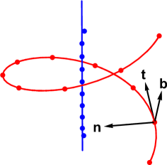
Figure 1: Frenet frame $\{{\bf t},{\bf n},{\bf b}\}$ at one point of the helicoidal curve defined in Eq. (33) (red solid line). Setting $R=1$ and $h=0.3$, the latter is shown for one turn, together with $N=11$ equidistantly spaced sampling points (red points). The blue line is the helix axis and the blue points correspond to the rotation centers ${\bf s}^{(c)}_{j}$ ($j=1,\ldots N-1$). The figure has been produced with the Mathematica software Wolfram Research Inc. (2014).

II.3 Numerical test

To test the numerical construction of Frenet frames, we consider a perfect helicoidal curve and compare the exact Frenet frames with the corresponding numerical approximations. The parametric representation of the curve is

$${\bf r}(\lambda)=\rho\cos(\lambda)\,{\bf e}^{(x)}+\rho\sin(\lambda)\,{\bf e}^{(y)}+h\lambda\,{\bf e}^{(z)},$$ (33)

where $\rho>0$ is the radius of the helix and its pitch is $p=h/2\pi$. Fig. 1 shows the form of the curve (33) for one complete turn (red line), setting $R=1$ and $h=0.3$ in arbitrary length units. Defining the matrix ${\bf F}(\lambda)=({\bf t}(\lambda),{\bf n}(\lambda),{\bf b}(\lambda))$, it follows from (33) that

$${\bf F}(\lambda)=\left(\begin{array}[]{ccc}-\frac{R\sin(\lambda)}{\sqrt{h^{2}+R^{2}}}&-\cos(\lambda)&\frac{h\sin(\lambda)}{\sqrt{h^{2}+R^{2}}}\\ \vskip 6.0pt plus 2.0pt minus 2.0pt\cr\frac{R\cos(\lambda)}{\sqrt{h^{2}+R^{2}}}&-\sin(\lambda)&-\frac{h\cos(\lambda)}{\sqrt{h^{2}+R^{2}}}\\ \vskip 6.0pt plus 2.0pt minus 2.0pt\cr\frac{h}{\sqrt{h^{2}+R^{2}}}&0&\frac{R}{\sqrt{h^{2}+R^{2}}}\\ \end{array}\right).$$ (34)

Using the method described in Section II.1, we construct numerical approximations $\tilde{{\bf F}}(\lambda_{j})$ of the Frenet bases (34) at $N=11$ equidistant sampling points, ${\bf R}_{j}$, which are shown as red dots in Fig. 1. From these Frenet bases we construct the axis points ${\bf s}^{(c)}_{j}$ (blue dots), which are shown together with the exact screw axis (blue line). For the first and the last axis point one notices a visible offset from the latter. We quantify the error of the numerically computed Frenet bases, $\tilde{{\bf F}}(\lambda_{j})$, as

$$\epsilon(j)=\sqrt{\text{tr}\left\{\mbox{\boldmath$\Delta$}(j)^{T}\cdot\mbox{\boldmath$\Delta$}(j)\right\}},$$ (35)

where

$$\mbox{\boldmath$\Delta$}(j)=\tilde{{\bf F}}(\lambda_{j})^{T}\cdot{\bf F}(\lambda_{j})-{\bf 1}.$$ (36)

For a perfect overlap of $\tilde{{\bf F}}(\lambda_{j})$ and ${\bf F}(\lambda_{j})$ one should have $\tilde{{\bf F}}(\lambda_{j})^{T}\cdot{\bf F}(\lambda_{j})={\bf 1}$, such that $\epsilon(j)=0$. We note that $\epsilon(j)$ is the Frobenius norm Golub and van Loan (1996) of $\mbox{\boldmath$\Delta$}(j)$. Fig. 2 shows $\epsilon(j)$ corresponding to the Frenet basis in Fig. 1 and confirms the slight offset of the first and last axis point from the ideal screw axis.

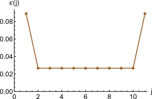
Figure 2: Overlap error (35) for the bases $\tilde{{\bf F}}(\lambda_{j})$ and ${\bf F}(\lambda_{j})$ at the red points in Fig. 1.

III Applications

In the following we consider two applications of the coarse-grained model for protein secondary structure, which has been described in the previous section and which will be referred to as ScrewFrame in the following. The first application concerns the construction of a tube model for a protein from the ScrewFrame parameters and in the second application, these parameters are used for a comparative study of ScrewFrame and DSSP for secondary structure assignment.

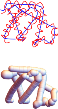
Figure 3: Top: $C_{\alpha}$-curve (red) of myoglobin (PDB code 1A6G) and B-spline curve (blue) linking the screw motion centers $\{{\bf s}^{(c)}_{j}\}$. Bottom: Tube representation of the $C_{\alpha}$-curve. The local tube radii equal the respective helix radii $\{\rho_{j}\}$ of the screw motions linking the Frenet frames $j$ and $j+1$ ($j=1,\ldots,N-1$). The figure has been produced with the Mathematica software Wolfram Research Inc. (2014).

III.1 Tube representation of a protein

As a first application we consider the ScrewFrame model for myoglobin, which is an oxygen-binding protein in muscular tissues. Myoglobin is composed of 151 amino acids which fold into a globular form and the dominant PSSEs are $\alpha$-helices. For our demonstration we use the crystallographic structure 1A6G of the Protein Data Bank Kirchmair et al. (2008). The red and blue line in the upper part of Fig. 3 display, respectively, the space curve defined by the positions ${\bf R}_{j}$ of the $C_{\alpha}$-atoms and the space curve linking the corresponding screw motion centers ${\bf s}^{(c)}_{j}$. Both space curves are constructed by a piecewise polynomial interpolation of second order Wolfram Research Inc. (2014). The blue line indicates the global fold of the protein, where ideal PSSEs appear simply as straight segments. In the following we refer to this line as the protein screw axis. It plays the same role as the “overall protein axis” in the P-Curve algorithm Sklenar et al. (1989), although its construction is different. The lower part of the figure shows the corresponding “tube model”, where the axis of the tube equals the protein screw axis and the local tube radius corresponds to the radius of the local screw motion. As in the original ScrewFit algorithm, the screw radius allows for a discrimination of different types of PSSEs (see Table 1).

	$\alpha$-helix	$\beta$-strand $\uparrow\uparrow$	$\beta$-strand $\uparrow\downarrow$	3-10 helix	$\pi$-helix
ScrewFit	0.165	0.061	0.051	0.122	0.165
ScrewFrame	0.227	0.098	0.080	0.187	0.227

Table 1: Screw radii in nm for standard model structures generated with Chimera Pettersen et al. (2004). Since ScrewFit uses the $C$-atoms in the peptide planes as reference points for the (pure) rotations, whereas as ScrewFrame uses the $C_{\alpha}$-atoms, the radii determined by ScrewFit are systematically smaller than those obtained from ScrewFrame.

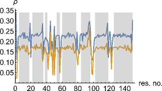
Figure 4: The radius $\rho$ for the ScrewFrame representation (blue line) of myoglobin (PDB code 1A6G) as a function of the residue number and the corresponding values for ScrewFit (brown line). The light gray stripes indicate the $\alpha$-helices found by DSSP.

Fig. 4 displays this quantity for myoglobin as a function of the residue number (blue line) and, for comparison, the corresponding values for the ScrewFit algorithm (brown line). The light gray stripes indicate $\alpha$-helices found by the DSSP algorithm. The comparison of the results with the ScrewFit analysis of the same protein structure shows that both methods indicate $\alpha$-helices in the same place, in close agreement with DSSP. Here it must be observed that the definition of the screw radii is not the same for ScrewFit and ScrewFrame. The rotation centers in the ScrewFit algorithm are the $C$-atoms in the $C-O-N$-peptide planes, whereas the $C_{\alpha}$-atoms are used for ScrewFrame. For an ideal $\alpha$-helix the corresponding radii are 0.165 nm and 0.227 nm, respectively (see Table 1). Fig. 5 shows the regularity measure (32) which plays an important role in the attribution of secondary structure elements to be discussed in the following section.

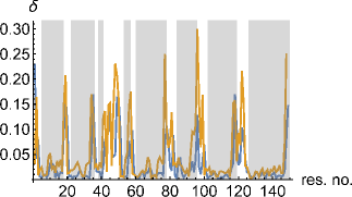
Figure 5: The regularity measure (32) for the ScrewFrame representation of myoglobin (PDB code 1A6G) as a function of the residue number and the corresponding values for ScrewFit (brown line). The light gray stripes indicate the $\alpha$-helices found by DSSP.

III.2 Analysis of the ASTRAL database

In order to compare our C_α based helicoidal analysis with the original ScrewFit method based on peptide planes Kneller and Calligari (2006); Calligari and Kneller (2012), we applied both methods to the “all $\alpha$ and “all $\beta$” categories of the ASTRAL subset of the SCOPe database Fox et al. (2013), using the ASTRAL SCOPe 2.04 subset with less than 40% sequence identity. In order to be able to work efficiently with such a large collection of protein structures, we constructed an ActivePaper Hinsen (2014a) containing the structures of the ASTRAL entries in MOSAIC format Hinsen (2014b). This file is available for download Hinsen (2014c). In addition to the ASTRAL database of real protein structures, we use ideal secondary-structure elements ($\alpha$-helix, $\pi$-helix, $3-10$-helix, parallel and anti-parallel $\beta$-strands) for polyalanine, which were constructed using the program Chimera Pettersen et al. (2004).

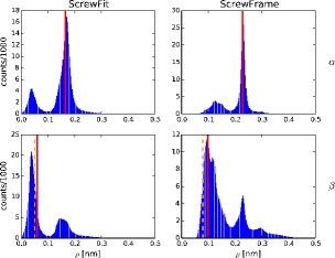
Figure 6: The helix radius $\rho$ for the all-$\alpha$ (top) and the all-$\beta$ structures (bottom), using the ScrewFit (left) and ScrewFrame (right) methods. Note that the ScrewFit radius is based on the C-atoms, whereas the ScrewFrame radius corresponds to the C_α-atoms, which explains the different values. The vertical lines indicate the values for ideal secondary-structure elements. For $\beta$-strands, there are two ideal values, one for parallel (red, drawn-out) and one for antiparallel (orange, dashed) strands.

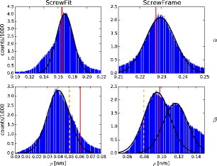
Figure 7: The helix radius $\rho$ around the ideal-$\alpha$ value for the all-$\alpha$ subset (top) and around the ideal-$\beta$ values for the the all-$\beta$ structures (bottom), using the ScrewFit (left) and ScrewFrame (right) methods. The vertical lines indicate values for ideal secondary-structure elements, as in Fig. 6. The Gaussian distributions fitted to the peaks are drawn in black, their parameters are given in Table 2. The $\beta$ distribution for ScrewFrame can be well described as a superposition of two Gaussian distributions, corresponding to parallel and antiparallel strands. The ScrewFit method cannot resolve this difference.

We also compare to DSSP secondary structure assignments for this database, using our own implementation of the DSSP algorithm which follows the description in the original publication Kabsch and Sander (1983) but, like the current version 2 of the DSSP software Hekkelman (2013), computes an ideal position for the backbone hydrogen positions instead of using experimental values, even if the latter are available.

As a first step, we compute ScrewFit and ScrewFrame parameters for all structures in the all-$\alpha$ and all-$\beta$ subsets of the ASTRAL database. In order to avoid inaccuracies introduced by the third-order approximations given by Eqs. (8)–(11), we do not compute Frenet frames for the first and last residue of each chain. For structures with missing residues, we compute the parameters for each continuous chain segment separately. Since the input structures are dominated by $\alpha$-helices and $\beta$-strands, respectively, we expect the distribution of our parameters to show clear peaks that correspond to these secondary structure elements.

The most important helix parameter for secondary structure description is the helix radius $\rho$, whose distribution in the ASTRAL database is shown in Fig. 6. The vertical lines show for comparison the values for ideal $\alpha$-helices and $\beta$-strands. For the $\beta$-strands, the red drawn-out lines stand for parallel and the orange dashed lines for antiparallel strands. A more detailed view is given in Fig. 7, which shows only the region around the dominant peak for each histogram, together with Gaussian distributions fitted to the peaks. The peaks are rather well described by a Gaussian, and the ScrewFrame method even allows to resolve the difference between parallel and antiparallel $\beta$-strands.

Whereas the average $\rho$ value for $\alpha$-helices is close to the value for an ideal helix, this is not the case at all for $\beta$-strands. This can be understood by looking at the distribution of the number of amino acids per full turn, $\tau$, shown in Fig. 8. Since the rotation angle is by definition in the interval $[-\pi\ldots\pi]$, the minimal value of $\tau$ is 2. This is also the value that describes an ideal $\beta$-strand, which is a flat structure. Any deviation from the ideal $\beta$-strand has a larger $\tau$, and because $\rho$ and $\tau$ are not independent (the length of the curve arc linking two neighboring C_α atoms is nearly constant), the deviation in $\rho$ from the ideal value is asymmetric as well.

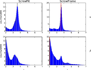
Figure 8: The number of amino acid residues per full turn, $\tau$, for the all-$\alpha$ (top) and the all-$\beta$ structures (bottom) using the ScrewFit (left) and ScrewFrame (right) methods. The theoretical minimal value of $\tau=2$ is very close to the observed value for $\beta$-sheets.

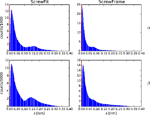
Figure 9: The regularity measure $\delta$ defined in Eq. (32) for the all-$\alpha$ and the all-$\beta$ subset of the ASTRAL data base (top and bottom, respectively).

The regularity measure $\delta$, defined in Eq. (32), is shown in Fig. 9. It shows that the ScrewFrame secondary structure elements are more regular than those identified by ScrewFit, in particular for structures dominated by $\alpha$-helices. We do not show here the distributions of the other parameters defined in the initial ScrewFit publication Kneller and Calligari (2006), but they are included in the electronic supplementary material. We note that the parameter distributions are in general narrower and thus better defined for ScrewFrame than for ScrewFit. We attribute this fact to fluctuations in the orientations of the peptide plans that have no impact on the C_α geometry.

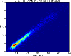
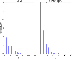
Figure 10: Top: A two-dimensional histogram comparing the total number of residues inside $\alpha$-helices as identified by ScrewFrame and DSSP. The strong localization of the distribution around the diagonal shows the similarity between these two assignments. Bottom: The distribution of the lengths of identified $\alpha$-helices, left for DSSP, right for ScrewFrame. The fatter tail for DSSP and the larger number of short helices for ScrewFrame are due to the fact that ScrewFrame breaks up strongly deformed helices into several pieces, whereas DSSP considers them a single helix.

We use the Gaussian distributions shown in Fig. 7 as the basis for defining secondary-structure elements. We define an $\alpha$-helix as a sequence of at least four consecutive C_α atoms whose screw transformations satisfy

$$\frac{|\rho-\mu_{\rho}|}{\sigma_{\rho}} < 3$$ (37)

$$\delta < 0.02\,\mbox{nm}$$ (38)

where $\mu_{\rho}$ and $\sigma_{\rho}$ are the mean value and standard deviation of the Gaussian distribution for the $\alpha$ peak in Fig. 7. The numerical values of these parameters are shown in Table 2.

	$\alpha$-helix	$\beta$-strand $\uparrow\uparrow$	$\beta$-strand $\uparrow\downarrow$
$\mu_{\rho}$	0.230	0.116	0.095
$\sigma_{\rho}$	0.007	0.014	0.015

Table 2: The parameters of the Gaussians fitted to the peaks in the distributions of the ScrewFrame parameter $\rho$ (see Fig. 7). All values are in units of nm.

We define a $\beta$-strand as a segment of consecutive C_α atoms whose screw transformations satisfy

$$\min\left(\frac{|\rho-\mu_{\rho}^{(1)}|}{\sigma_{\rho}^{(1)}},\frac{|\rho-\mu_{\rho}^{(2)}|}{\sigma_{\rho}^{(2)}}\right) < 1$$ (39)

$$\delta < 0.08\,\mbox{nm}$$ (40)

where $\mu_{\rho}^{(1/2)}$ and $\sigma_{\rho}^{(1/2)}$ are the mean values and standard deviations of the Gaussian distributions for the parallel and antiparallel $\beta$ peaks in Fig. 7. The numerical parameters in these definitions were chosen to make our definitions match the secondary structure assignments made by the DSSP method.

There is a fundamental difference between our approach and the DSSP method for defining $\beta$-strands. The ScrewFrame approach looks for a regular structure along the peptide chain, whereas the DSSP method identifies hydrogen bonds between the strands that make up a $\beta$-sheet. ScrewFrame thus finds individual strands, which can be paired up to identify sheets in a separate step. A strand must consist of at least three consecutive residues in order to be considered regular; in fact, the regularity measure $\delta$ is defined in terms of the difference of two consecutive screw transformations, each of which connects two residues. DSSP needs to look at two strands simultaneously in order to identify $\beta$ structures, but has no minimal length condition and in fact admits $\beta$-sheets as mall as a single h-bonded residue pair. For practically relevant $\beta$-sheets in real protein structures, these differences are, however, not important, but they must be understood for interpreting the following comparison between the two methods.

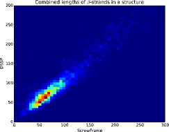
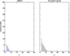
Figure 11: Top: A two-dimensional histogram comparing the total number of residues inside $\beta$-strands as identified by ScrewFrame and DSSP. The strong localization of the distribution around the diagonal shows the similarity between these two assignments. Bottom: The distribution of the lengths of identified $\beta$-helices, left for DSSP, right for ScrewFrame. The peak at very short strands in the DSSP distribution is absent from the ScrewFrame results because ScrewFrame needs at least three consecutive residues to recognize a regular structure.

A one-to-one comparison of secondary structure elements from two different assignment methods is not of particular interest, because an exact match is the exception rather than the rule. The inherent fuziness of secondary structure definitions leads to arbitrary choices and thus inevitable differences. The most frequent deviation between two assignments is the end points of secondary structure elements, where a difference of one or two residues is common and acceptable. Another frequent deviation concerns deformed secondary structure elements, which one method may identify as a single element whereas another one recognizes it as multiple distinct elements.

We therefore chose a statistical comparison to compare the ScrewFrame results to those of DSSP, which is shown in Figs. 10 for $\alpha$-helices and 11 for $\beta$-strands. We consider two quantities: (1) the total number of residues of a given structure which are inside a recognized secondary-structure element, and (2) the length of each individual secondary-structure element. We compute the first quantity for both methods and show their joint distribution (upper plot in the two figures). For the vast majority of structures, the two residue counts are close to equal, which means that neither method yields systematically more or longer secondary-structure elements than the other. The lower plots show the distributions of the lengths of individual secondary-structure elements. For $\alpha$-helices, DSSP has a fatter tail (helices of length 20 or more), whereas ScrewFrame identifies a larger number of short helices. The reason for these differences is that ScrewFrame tends to split up kinked helices which DSSP identifies as single units. For $\beta$-strands, we notice that DSSP identifies many more very short elements. This is due to the different definitions: a single $\beta$-type hydrogen bond is sufficient to define a $\beta$-sheet in DSSP, but ScrewFrame requires at least three consecutive residues to identify any regular structure.

IV Conclusion and Outlook

We have presented a generalization of the ScrewFit method for protein structure assignment and description, which uses only the positions of the $C_{\alpha}$-atoms along the protein backbone. As in the ScrewFit approach, the global protein fold is described as a succession of screw motions relating consecutive recurrent motifs along the protein backbone, but the “motifs” are here the tripods (planes) formed by the three (two) orthonormal vectors of the local Frenet bases to the $C_{\alpha}$ space curve. Despite the fact that ScrewFrame uses less information than ScrewFit, all standard PSSEs are recognized on the basis of thresholds for the local screw radii and a suitably defined regularity measure. ScrewFrame even permits to distinguish between parallel and antiparallel $\beta$-strands, which the classical ScrewFit method fails to do. A thorough comparison with the commonly used DSSP method on the assignment of PSSEs in the ASTRAL database shows that both methods yield very similar results for the total amount of PSSEs. ScrewFrame tends, however, to break long helices into smaller pieces, such that the length distribution of PSSEs is different. Due to the minimalistic character of the geometrical model for protein folds, the evaluation of the ScrewFrame model parameters is very efficient. This allows for working with protein structure databases and for analyzing simulated molecular dynamics trajectories of proteins. ScrewFrame may also be used a starting point for the development of minimalistic models for protein structure and dynamics, similar to the wormlike chain model Doi and Edwards (1986), which has been successfully applied to DNA Marko and Siggia (1995). As already mentioned, our method can also be used to analyze dynamical processes, such as the folding and unfolding of peptides Spampinato and Maccari (2014) and it can describe the fold of intrinsically disordered proteins.

An ActivePaper Hinsen (2014a) containing all the software, input datasets, and results from this study is available as supplementary material. The datasets can be inspected with any HDF5-compatible software, e.g. the free HDFView.The HDF Group (2013) Running the programs on different input data requires the ActivePaper software Hinsen (2014a).

References

- Pauling and Corey (1951) L. Pauling and R. B. Corey, P Natl Acad Sci USA 37, 729 (1951).
- Pauling et al. (1951) L. Pauling, R. B. Corey, and H. R. Branson, P Natl Acad Sci USA 37, 205 (1951).
- Kabsch and Sander (1983) W. Kabsch and C. Sander, Biopolymers 22, 2577 (1983).
- Frishman and Argos (1995) D. Frishman and P. Argos, Proteins 23, 566 (1995).
- Kneller and Calligari (2006) G. R. Kneller and P. Calligari, Acta Crystallogr D 62, 302 (2006).
- Calligari and Kneller (2012) P. A. Calligari and G. R. Kneller, Acta Crystallogr D 68, 1690 (2012).
- Chandonia et al. (2004) J.-M. Chandonia, G. Hon, N. S. Walker, L. Lo Conte, P. Koehl, M. Levitt, and S. E. Brenner, Nucleic Acids Research 32, D189 (2004).
- Sklenar et al. (1989) H. Sklenar, C. Etchebest, and R. Lavery, Proteins 6, 46 (1989).
- Grimes et al. (1999) J. M. Grimes, S. D. Fuller, and D. I. Stuart, Acta Crystallogr D 55, 1742 (1999).
- Marabini et al. (2013) R. Marabini, J. R. Macias, J. Vargas, A. Quintana, C. O. S. Sorzano, and J. M. Carazo, Acta Crystallogr D 69, 695 (2013).
- Tozzini (2005) V. Tozzini, Curr. Opin. Struct. Biol. 15, 144 (2005).
- Levitt and Greer (1977) M. Levitt and J. Greer, J Mol Biol 114, 181 (1977).
- Dupuis et al. (2004) F. Dupuis, J.-F. Sadoc, and J.-P. Mornon, Proteins 55, 519 (2004).
- Labesse et al. (1997) G. Labesse, N. Colloc’h, J. Pothier, and J.-P. Mornon, Computer applications in the biosciences: CABIOS 13, 291 (1997).
- Park et al. (2011) S.-Y. Park, M.-J. Yoo, J.-M. Shin, and K.-H. Cho, BMB Reports 44, 118 (2011).
- Hu et al. (2011) S. Hu, M. Lundgren, and A. J. Niemi, Phys Rev E 83, 061908 (2011).
- Altmann (1986) S. Altmann, Rotations, Quaternions, and Double Groups (Clarendon Press, Oxford, 1986).
- Chasles (1830) M. Chasles, Bulletin des Sciences Mathématiques, Astronomiques, Physiques et Chimiques 14, 321 (1830).
- Kneller (1991) G. R. Kneller, Mol Simulat 7, 113 (1991).
- Wolfram Research Inc. (2014) Wolfram Research Inc., Mathematica, Version 10.0 (Wolfram Research Inc., Champaign, Illinois, USA, 2014).
- Golub and van Loan (1996) G. Golub and C. van Loan, Matrix Computations (The John Hopkins University Press, 1996).
- Kirchmair et al. (2008) J. Kirchmair, P. Markt, S. Distinto, D. Schuster, G. Spitzer, K. Liedl, T. Langer, and G. Wolber, J. Med. Chem 51, 7021 (2008).
- Pettersen et al. (2004) E. F. Pettersen, T. D. Goddard, C. C. Huang, G. S. Couch, D. M. Greenblatt, E. C. Meng, and T. E. Ferrin, J Comput Chem 25, 1605 (2004).
- Fox et al. (2013) N. K. Fox, S. E. Brenner, and J. M. Chandonia, Nucleic Acids Research 42, D304 (2013).
- Hinsen (2014a) K. Hinsen, ActivePapers, http://www.activepapers.org/ (2014a).
- Hinsen (2014b) K. Hinsen, Journal of chemical information and modeling 54, 131 (2014b).
- Hinsen (2014c) K. Hinsen, ASTRAL-SCOPe subset 2.04 in ActivePapers format (2014c), URL http://dx.doi.org/10.5281/zenodo.11086.
- Hekkelman (2013) M. Hekkelman, DSSP 2.2.1, http://swift.cmbi.ru.nl/gv/dssp/ (2013).
- Doi and Edwards (1986) M. Doi and S. Edwards, The Theory of Polymer Dynamics (Oxford University Press, New York, 1986).
- Marko and Siggia (1995) J. F. Marko and E. D. Siggia, Macromolecules 28, 8759 (1995).
- Spampinato and Maccari (2014) G. Spampinato and G. Maccari, J Chem Theory Comput 10, 3885 (2014).
- The HDF Group (2013) The HDF Group, HDFView, http://www.hdfgroup.org/hdf-java-html/hdfview/ (2013).