Ramified covers and tame isomonodromic solutions on curves

Abstract.

In this paper, we investigate the possibility of constructing isomonodromic deformations by ramified covers. We give new examples and prove a classification result.

Introduction

Let $X$ be a complete curve of genus $g$ over $\mathbb{C}$ and $D$ be a reduced divisor on $X$: $D=[x_{1}]+\cdots+[x_{n}]$ is equivalent to the data of $n$ distinct points on $X$. Set $N:=3g-3+n$; when $N>0$, that we will assume along the paper, then $N$ is the dimension of the deformation space $M_{g,n}$ of the pair $(X,D)$.

Let $(E,\nabla)$ be a rank $2$ logarithmic connection over $X$ with polar divisor $D$. In other words, $E\to X$ is a rank $2$ holomorphic vector bundle and $\nabla:E\to E\otimes\Omega^{1}_{X}(D)$ a linear meromorphic connection having simple poles at the points of $D$. By considering the analytic continuation of a local basis of $\nabla$-horizontal sections of $E$, we inherit a monodromy representation

$$\rho_{\nabla}\ :\ \pi_{1}(X\setminus D)\to\mathrm{GL}_{2}(\mathbb{C})$$

(which is well-defined up to conjugacy in $\mathrm{GL}_{2}(\mathbb{C})$).

Given a deformation $t\mapsto(X_{t},D_{t})$ of the complex structure, there is a unique deformation $t\mapsto(X_{t},D_{t},E_{t},\nabla_{t})$ up to bundle isomorphism such that the monodromy is constant. For $t$ varrying in the Teichmuller space $T_{g,n}$, we get the universal isomonodromic deformation (see [9]). Considering the moduli space $\mathcal{M}_{g,n}$ of quadruples $(X,D,E,\nabla)$, isomonodromic deformations define the leaves of a $N$-dimensional foliation transversal to the natural projection

$$\mathcal{M}_{g,n}\to M_{g,n}\ ;\ (X,D,E,\nabla)\mapsto(X,D).$$

The corresponding differential equation is explicitely described in [13] (via local analytic coordinates on $M_{g,n}$) and is known to be polynomial with respect to the algebraic structure of $\mathcal{M}_{g,n}$ (it is the non-linear Gauss-Manin connection constructed in [25, section 8]). In the case $g=0$, we get the Garnier system (see [23]), and for $n=4$, the Painlevé VI equation. Solutions (or leaves) are generically transcendental and it is expected that the transcendence increase with $N$ (see [8, Introduction] for instance). However, there are some tame solutions.

Algebraic solutions of Painlevé VI equation were recently classified in [2, 14]. Some algebraic solutions are constructed in [5] for the Garnier case; see the discussion in the introduction of [6] for higher genus case.

Some solutions, called “classical”, reduce to solutions of linear differential equations. They are classified in the Painlevé case in [27]. In the Garnier case, such solutions arise by considering deformations of reducible connections (see [24, 21]): they can be expressed in terms of Lauricella hypergeometric functions.

There are also “tame solutions” coming from simpler isomonodromy equations (e.g. with lower $n$ or $g$) . In [21], it is proved that, one way of reducing $n$ (when $g=0$) is to consider those deformations having scalar local monodromy around some pole. There is another way of reduction, by using ramified covers, and this is what we want to investigate in this note.

1. Known constructions via ramified covers

Ramified covers of curves have already been used to construct algebraic solutions of the Painlevé VI equation (see [7, 1]) and Garnier systems (see [5]). But they have also been used to understand relations between transcendental solutions.

1.1.

The most classical case is the quadratic transformation of the Painlevé VI equation (see [12, 19, 26, 22]). We consider a deformation $t\mapsto(E_{t},\nabla_{t})$ of a rank $2$ connection on $\mathbb{P}^{1}$ with simple poles at $(x_{1},x_{2},x_{3},x_{4})=(0,1,t,\infty)$. At a pole $x_{i}$, we consider eigenvalues $\theta_{i}^{1},\theta_{i}^{2}$ of the residual matrix and call exponent the difference $\theta_{i}:=\theta_{i}^{1}-\theta_{i}^{2}$ (defined up to a sign). To be concrete, if all $\theta_{i}^{1}+\theta_{i}^{2}=0$ and the connection is irreducible, then $E_{t}$ is the trivial bundle except for a discrete set of parameters (see [3]) and the connection is just defined by a two-by-two system. If moreover exponents satisfy

$$\theta_{0}=\theta_{\infty}=\frac{1}{2}$$

then after lifting the connection on the two-fold cover

$$\mathbb{P}_{\tilde{x}}^{1}\to\mathbb{P}_{x}^{1}\ ;\ \tilde{x}\mapsto\tilde{x}^{2}$$

we get a connection $(\tilde{E}_{t}^{0},\tilde{\nabla}_{t}^{0})$ having $6$ simple poles at

$$\tilde{x}=0,\ \pm 1,\ \pm\sqrt{t}\ \text{and}\ \infty$$

(see figure 1).

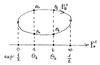
Figure 1. Quadratic transformation’s cover

Those two poles at ramification points $\tilde{x}=0,\infty$ have now integral exponents and therefore scalar local monodromy $-I$. These singular points are “apparent”, i.e. can be erased by a combination of

• a rational gauge (i.e. birational bundle) transformation,

• the twist by a rank $1$ connection.

This can be done taking into account the deformation, and we get a new deformation $t\mapsto(\tilde{E}_{t},\tilde{\nabla}_{t})$ of a rank $2$ connection with $4$ simple poles $\tilde{x}=\pm 1$ and $\pm\sqrt{t}$ on the Riemann sphere $\mathbb{P}_{\tilde{x}}^{1}$. This new deformation is clearly isomonodromic if the initial deformation was. Taking into account the exponents, we get a rational two-fold cover

$$\mathrm{Quad}\ :\ \mathcal{M}_{0,4}(\frac{1}{2},\theta_{1},\theta_{t},\frac{1}{2})\ \stackrel{{\scriptstyle 2:1}}{{\longrightarrow}}\ \mathcal{M}_{0,4}(\theta_{1},\theta_{1},\theta_{t},\theta_{t})$$

between moduli spaces that conjugates isomonodromic foliations. The map $\mathrm{Quad}$ is called quadratic transformation of the Painlevé VI equation.

1.2.

When exponents satisfy $\theta_{0}=\theta_{1}=\theta_{\infty}=\frac{1}{2}$, we can iterate twice the map (after conveniently permuting the poles) and we get the quartic transformation

$$\mathrm{Quad}\circ\mathrm{Quad}\ :\ \mathcal{M}_{0,4}(\frac{1}{2},\frac{1}{2},\theta_{t},\frac{1}{2})\ \stackrel{{\scriptstyle 4:1}}{{\longrightarrow}}\ \mathcal{M}_{0,4}(\theta_{t},\theta_{t},\theta_{t},\theta_{t}).$$

Finally, if we consider the Picard parameters $\theta_{0}=\theta_{1}=\theta_{t}=\theta_{\infty}=\frac{1}{2}$ for Painlevé VI equation, we can iterate arbitrary many times the quadratic tranformation. There is also a cubic transformation in this case (see [22]).

1.3.

For Picard parameters $(\theta_{0},\theta_{1},\theta_{t},\theta_{\infty})=(\frac{1}{2},\frac{1}{2},\frac{1}{2},\frac{1}{2})$ of Painlevé VI equation, one can modify the construction above as follows. Consider now the elliptic two-fold cover ramifying over the $4$ poles of $(E_{t},\nabla_{t})$

$$\phi_{t}\ :\ X_{t}=\{y^{2}=x(x-1)(x-t)\}\stackrel{{\scriptstyle 2:1}}{{\rightarrow}}\mathbb{P}^{1}_{x}\ ;\ (x,y)\mapsto x$$

and lift-up the connection on the elliptic curve. After birational gauge transformation, we get a holomorphic connection $(\tilde{E}_{t},\tilde{\nabla}_{t})$ that generically split as the direct sum of two holomorphic connections of rank $1$. This means that, for these parameters, Painlevé VI solutions actually parametrize isomonodromic deformations of rank $1$ connections over a family of elliptic curves. This allow to solve this very special element of Painlevé VI family (originally found by Picard) by means of elliptic functions (see [11, 20, 15]). By the way, we get a birational map

$$\mathcal{M}_{0,4}(\frac{1}{2},\frac{1}{2},\frac{1}{2},\frac{1}{2})\ \stackrel{{\scriptstyle\sim}}{{\longrightarrow}}\ \mathcal{M}_{1,0}$$

that commutes with isomonodromic flow.

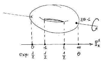
Figure 2. Lamé’s cover

1.4.

This map has been extended to Lamé parameters in [16, 17] as a birational transformation

$$\text{Lam\'{e}}\ :\ \mathcal{M}_{0,4}(\frac{1}{2},\frac{1}{2},\frac{1}{2},\theta_{\infty})\ \stackrel{{\scriptstyle\sim}}{{\longrightarrow}}\ \mathcal{M}_{1,1}(2\theta_{\infty}-1)$$

also commuting with isomonodromic flow (see figure 2).

1.5.

In [10], a $2$-fold ramified cover commuting with isomonodromic flow

$$\mathcal{M}_{0,6}(\frac{1}{2},\frac{1}{2},\frac{1}{2},\frac{1}{2},\frac{1}{2},\frac{1}{2})\ \stackrel{{\scriptstyle 2:1}}{{\longrightarrow}}\ \mathcal{M}_{2,0}$$

has been constructed by lifting connections on the hyperelliptic cover

$$\phi_{r,s,t}\ :\ X_{r,s,t}=\{y^{2}=x(x-1)(x-r)(x-s)(x-t)\}\ \stackrel{{\scriptstyle 2:1}}{{\longrightarrow}}\ \mathbb{P}^{1}_{x}\ ;\ (x,y)\mapsto x$$

(see figure 3).

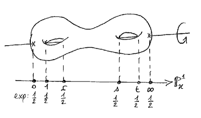
Figure 3. Genus $2$ cover

1.6.

However, for higher genus $g>2$ hyperelliptic curve, the similar map

$$\mathcal{M}_{0,2g+2}(\frac{1}{2},\ldots,\frac{1}{2})\ \longrightarrow\ \mathcal{M}_{g,0}$$

has small image: not only the deformation upstairs is reduced to the hyperelliptic locus (having codimension $g-2$), but even for a fixed hyperelliptic curve, the image has codimension $2(g-1)$ in the moduli space of connections.

2. Results

In this note, we classify all “interesting” maps that can be constructed between moduli spaces like above, using ramified covers of curves. Let us explain.

Let $(X,D^{\nabla},E,\nabla)$ be a logarithmic rank $2$ connections and $\phi:\tilde{X}\to X$ be a ramified cover. Let $D^{\phi}$ denotes the set of critical points of $\phi$ while $D^{\nabla}$ denotes the set of poles of $\nabla$; they will be not disjoint in many cases. Consider now the universal deformation $t\mapsto(X_{t},D_{t})$ of the marked curve $(X,D)$ where $D$ is the union of $D^{\phi}$ and $D^{\nabla}$. There is a unique local deformation $t\mapsto(X_{t},D_{t},E_{t},\nabla_{t},\phi_{t})$ where $t\mapsto(X_{t},D^{\nabla}_{t},E_{t},\nabla_{t})$ is isomonodromic, and $t\mapsto(X_{t},D^{\phi}_{t},\nabla_{t})$ is topologically trivial (we just deform the critical locus $D^{\phi}_{t}$). Fibers of the map $t\mapsto(X_{t},D^{\nabla}_{t})$ are algebraic deformations, so-called Hurwitz families.

The main remark is that the lift to $\tilde{X}_{t}$ of the connection:

$$t\mapsto(\tilde{E}_{t},\tilde{\nabla}_{t}):=\phi_{t}^{*}(E_{t},\nabla_{t})$$

is isomonodromic along the deformation. By applying rational gauge transformation and twisting with a rank $1$ isomonodromic deformation, we may assume that $(\tilde{E}_{t},\tilde{\nabla}_{t})$ is an isomonodromic deformation of logarithmic $\mathfrak{sl}_{2}$-connexion, free of apparent singular points. In fact, this is possible whenever $\nabla_{t}$ has an essential singular point, i.e. with monodromy. Let $\tilde{D}_{t}$ be the (reduced) polar divisor of $\tilde{\nabla}_{t}$ after deleting apparent singular points. Last but not least, assume that

• the connection $(E_{t},\nabla_{t})$, or equivalently $(\tilde{E}_{t},\tilde{\nabla}_{t})$, has Zariski dense monodromy,

• the deformation $t\mapsto(\tilde{X}_{t},\tilde{D}_{t},\tilde{E}_{t},\tilde{\nabla}_{t})$ induces a locally universal deformation $t\mapsto(\tilde{X}_{t},\tilde{D}_{t})$ of the marked curve.

These are the so-called “interesting” conditions. The second item means that we get a complete isomonodromic deformation after the construction. We thus get a complete parametrisation of a leaf of the isomonodromic foliation. All examples listed in section 1 are examples of such constructions. It is easy to construction many exemples where all conditions but the last one are satisfied. However, the last condition, saying that we get the complete deformation, is so hard to realized that we are able, in section 3, to classify all examples. This is our main result in this note. Appart from above known examples, we have the following three new cases.

2.1.

Let $s\mapsto X_{s}=\{y^{2}=x(x-1)(x-s)\}$ the Legendre family of elliptic curves and let $t\mapsto(E_{t},\nabla_{t})$ an isomonodromic deformation of a rank $2$ connection with poles located at $x=0,1,t,\infty$. More rigorously, we should say $\tilde{t}\mapsto(E_{t},\nabla_{t})$ where $\tilde{t}$ belongs to the Teichmuller space, given by the universal cover $T\to\mathbb{P}^{1}_{x}\setminus\{0,1,\infty\}$ in this case, and $t$ denotes the projection of $\tilde{t}$ on $\mathbb{P}^{1}_{x}\setminus\{0,1,\infty\}$. Now, assume that exponents of $\nabla_{t}$ take the form $(\theta_{0},\theta_{1},\theta_{t},\theta_{\infty})=(\frac{1}{2},\frac{1}{2},\theta,\frac{1}{2})$. Therefore, after lifting on the elliptic curve, we get a connection with $3$ apparent singular points and two copies of the singular point at $x=t$. By gauge transformation, we finally get a connection $(\tilde{E}_{s,t},\tilde{\nabla}_{s,t})$ with only two simple poles, but to get a $\mathfrak{sl}_{2}$-connection we need to shift one of the two exponents (see figure 4). We finally get a rational map

$$\mathbb{P}^{1}_{s}\times\mathcal{M}_{0,4}(\frac{1}{2},\frac{1}{2},\theta_{t},\frac{1}{2})\ \longrightarrow\ \mathcal{M}_{1,2}(\theta,\theta-1).$$

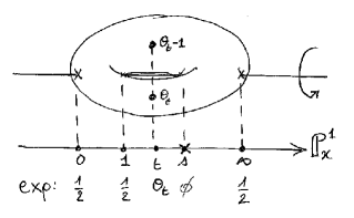
Figure 4. Ruled deformations via uncomplete elliptic cover

Each isomonodromic deformation thus obtained is parametrized by a combination of a Painlevé VI solution (variable $t$) and a rational function (variable $s$). We get a $2$-parameter space of such tame isomonodromic deformations; they form a codimension $2$ subset in $\mathcal{M}_{1,2}(\theta,\theta-1)$, the image of the map above, which is saturated by the isomonodromic foliation. The leaves belonging to this set are ruled surfaces parametrized by a Painlevé transcendent. One should recover the Lamé case of section 1 by restricting the isomonodromic foliation to the locus $s=t$. We postpone the careful study of this picture to another paper.

2.2.

Consider now the family of genus $2$ curves given by

$$(s,t)\mapsto X_{s,t}=\{y^{2}=x(x-1)(x-s)(x-t_{1})(x-t_{2})\},\ \ \ s\in\mathbb{C},\ t=(t_{1},t_{2})\in\mathbb{C}^{2}$$

together with the hyperelliptic cover (see figure 5)

$$\phi_{s,t}:X_{s,t}\to\mathbb{P}^{1}_{x}\ ;\ (x,y)\mapsto x.$$

Let $t\mapsto(E_{t},\nabla_{t})$ be an isomonodromic deformation of a rank $2$ connection on $\mathbb{P}^{1}_{x}$ with poles located at five among the six critical values, namely $x=0,1,t_{1},t_{2},\infty$. Assume that all exponents of $\nabla_{t}$ take the form $\theta_{0}=\theta_{1}=\theta_{t_{1}}=\theta_{t_{2}}=\theta_{\infty}=\frac{1}{2}$.

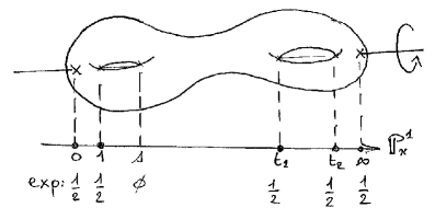
Figure 5. Ruled deformations via uncomplete hyperelliptic cover

After lifting the connection to the curve $X_{s,t}$, deleting apparent singular points by gauge transformation, we get a $\mathfrak{sl}_{2}$-connection on $X_{s,t}$ with a single apparent singular point located at $x=\infty$. This provides a rational map

$$\mathbb{P}^{1}_{s}\times\mathcal{M}_{0,5}(\frac{1}{2},\ldots,\frac{1}{2})\ \longrightarrow\ \mathcal{M}_{2,1}(1)$$

conjugating isomonodromic foliations. Here, the only singular point is apparent and it is not possible to delete it. We can just choose to place it at $x=\infty$; it is irrelevant for the deformation. Again, isomonodromic deformations obtained by this way are parametrized by rank $2$ Garnier solutions ($(t_{1},t_{2})$ variables) combined with a rational function of $s$. Again, the corresponding leaves of the isomonodromic foliation are uniruled and form a codimension $2$ set.

2.3.

Finally, consider the Legendre family $t_{1}\mapsto X_{t_{1}}=\{y^{2}=x(x-1)(x-t_{1})\}$ of elliptic curves and let $t=(t_{1},t_{2})\mapsto(E_{t},\nabla_{t})$ an isomonodromic deformation of a rank $2$ connection with poles located at $x=0,1,t_{1},t_{2},\infty$. Assume that exponents of $\nabla_{t}$ take the form $(\theta_{0},\theta_{1},\theta_{t_{1}},\theta_{t_{2}},\theta_{\infty})=(\frac{1}{2},\frac{1}{2},\frac{1}{2},\theta,\frac{1}{2})$. After lifting and applying gauge transformation, we get a $\mathfrak{sl}_{2}$-connection on the elliptic curve $X_{t_{1}}$ with two simple poles over $x=t_{2}$ having same exponent $\theta$. This gives us a rational map

$$\Phi_{\theta}\ :\ \mathcal{M}_{0,5}(\frac{1}{2},\frac{1}{2},\frac{1}{2},\theta,\frac{1}{2})\ \longrightarrow\ \mathcal{M}_{1,2}(\theta,\theta)$$

conjugating isomonodromic foliations (see figure 6). We study this map from the topological (i.e. monodromy) point of view in section 4 and deduce

Theorem 1.

The map $\Phi_{\theta}$ is dominant and generically two-to-one.

In other word, almost all rank $2$ logarithmic connections with two poles on an elliptic curve is a pull-back of a rank $2$ logarithmic connection on $\mathbb{P}^{1}$; in particular, such connections are invariant (up to gauge equivalence) under the hyperelliptic involution permuting the two poles. This construction can be thought as intermediate between the genus two case and the Lamé case of section 1. This is a reminiscence of the hyperelliptic nature of the twice-punctured torus.

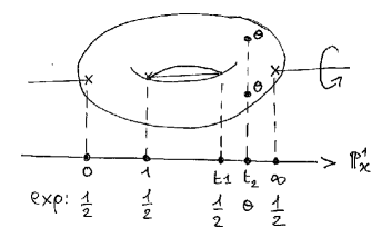
Figure 6. The two punctured torus

2.4. Classification

We prove in section 3 the following

Theorem 2.

Let $t\mapsto(X_{t},D_{t},E_{t},\nabla_{t})$ be an isomonodromic deformation of logarithmic $\mathfrak{sl}_{2}$-connections. Let $\phi_{t}:\tilde{X}_{t}\to X_{t}$ a family of ramified covers. Assume that the pull-back deformation $t\mapsto(\tilde{X}_{t},\tilde{D}_{t},\tilde{E}_{t},\tilde{\nabla}_{t})$ after deleting apparent singular points is locally universal, i.e. the corresponding map $t\mapsto(\tilde{X}_{t},\tilde{D}_{t})$ is locally surjective. In particular, the deformation has dimension $\geq 3\cdot\mathrm{genus}(\tilde{X}_{t})-3+\deg(\tilde{D}_{t})$. Then we are in one of the following cases:

• The monodromy of $\nabla_{t}$ (or equivalently $\tilde{\nabla}_{t}$) is finite, reducible or dihedral.

• The deformation $t\mapsto(X_{t},D_{t},E_{t},\nabla_{t})$ is actually trivial, and we get an algebraic isomonodromic deformation by deforming $\phi_{t}$. Up to gauge transformation, we are in the list of Doran [7] or Diarra [5]. In particular, $(X_{t},D_{t},E_{t},\nabla_{t})$ is a rigid hypergeometric system ($X_{t}=\mathbb{P}^{1}$, $\deg(D_{t})=3$) and $\deg(\phi_{t})\leq 18$.

• The deformation $t\mapsto(X_{t},D_{t},E_{t},\nabla_{t})$ is non trivial, $X_{t}=\mathbb{P}^{1}$, $\deg(\phi_{t})=2$ or $4$, and we are in one of the constructions described in sections 1.1, 1.2, 1.4, 1.5, 2.1, 2.2 and 2.3.

2.5. Complement

In the last section, we complete the picture of section 2.3 when $\theta=\frac{1}{2}$ by constructing a rational map

$$\Psi\ :\ \mathcal{M}_{1,2}(\frac{1}{2},\frac{1}{2})\ \longrightarrow\ \mathcal{M}_{2,0}$$

that conjugates isomonodromic foliations. In order to explain, consider the “bi-elliptic cover”

where $\phi_{i}:X_{i}\to\mathbb{P}^{1}_{x}$ is the elliptic two-fold cover branching over $x=0,1,t_{i},\infty$, for $i=1,2$, and the remaining part of the diagramm is the fiber product of $\phi_{1}$ and $\phi_{2}$. In particular, $\tilde{X}_{t_{1},t_{2}}$ has genus $2$ and each $\pi_{i}:\tilde{X}_{t_{1},t_{2}}\to X_{i}$ is a two-fold cover branching over the two points $\phi_{i}^{-1}(t_{j})$ (where $\{i,j\}=\{1,2\}$). By the way, $\phi:\tilde{X}_{t_{1},t_{2}}\to\mathbb{P}^{1}_{x}$ is a $4$-fold cover ramifying over all five points $x=0,1,t_{1},t_{2},\infty$.

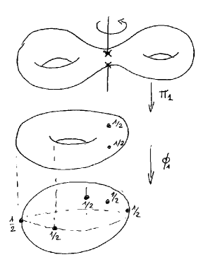
Figure 7. Bi-elliptic cover

The map $\Phi_{\theta}$ of section 2.3 comes from the elliptic covering $\pi_{1}$, while the map $\Psi$ above, from $\phi_{1}$ in the bi-elliptic diagramm. In Theorem 11, we characterize the image of $\Psi$ and

$$\Psi\circ\Phi_{\frac{1}{2}}\ :\ \mathcal{M}_{0,5}(\frac{1}{2},\ldots,\frac{1}{2})\ \longrightarrow\ \mathcal{M}_{2,0}$$

in terms of the monodromy representation. Mind that, contrary to the previous constructions, we do not get complete isomonodromic deformations (of holomorphic $\mathfrak{sl}_{2}$-connections on genus $2$ curves) but isomonodromic deformations over the codimension $1$ bi-elliptic locus in the moduli space $M_{2,0}$.

This last construction was inspired by [18], where isomonodromic deformations of dihedral logarithmic $\mathfrak{sl}_{2}$-connections are constructed in $\mathcal{M}_{1,2}(\frac{1}{2},\frac{1}{2})$ as direct image of rank $1$ holomorphic connections on the bi-elliptic cover $X_{t_{1},t_{2}}$.

3. Classification of covers

Here, we follow ideas of [5, 6], replacing connections by their underlying orbifold structure à la Poincaré.

Let $\phi:\tilde{X}\to X$ be a ramified cover where $X$ is a genus $g$ hyperbolic orbifold with $n$ singularities of order $2\leq\nu_{1}\leq\cdots\leq\nu_{n}\leq\infty$ (i.e. having angle $\alpha_{i}=\frac{2\pi}{\nu_{i}}$). Pulling-back by $\phi$, we get a branched orbifold structure on $\tilde{X}$: orbifold points have angle $\tilde{\alpha}=\frac{2\pi k}{\nu}$ where $k$ is the branching order of $\phi$ (i.e. $\phi\sim z^{k}$) and

• $\nu=\nu_{i}$ over $i^{\text{t}h}$ orbifold point of $X$,

• $\nu=1$ over a regular point.

Denote by $\tilde{g}$ the genus of $\tilde{X}$, and by $b$ the number of branching points on $\tilde{X}$.

The volume of $X$ with respect to the orbifold metric is given by

$$\mathrm{aire}(X)=2\pi(2g-2)+\sum_{i=1}{n}(2\pi-\alpha_{i});$$

we get the analogous formula for $\tilde{X}$ with respect to the pull-back metric (even if $\alpha_{i}$ need not be $<2\pi$) and $\mathrm{aire}(\tilde{X})=d\cdot\mathrm{aire}(X)$ where $d=\deg(\phi)$. This yields (after division by $2\pi$)

(1) $$d\cdot\left(2g-2+\sum_{i=1}^{n}\left(1-\frac{1}{\nu_{i}}\right)\right)\ \leq\ 2\tilde{g}-2+\sum_{j=1}^{\tilde{n}}\left(1-\frac{k_{j}}{\nu_{i(j)}}\right)-b$$

If branching points are simple (with branching order $2$) then we get an equality.

We want to classify cases for which, by deforming simultaneously $X$ and $\phi$, we get the local universal deformation of $\tilde{X}$. The dimension of the deformation space of $X$ is given by $3g-3+n\geq 0$ (positivity ollows from hyperbolicity). For $\tilde{X}$, since we are more involved in the differential equation than in the orbifold structure, we do not take into account the branching points in the deformation, and dimension is given by $3\tilde{g}-3+\tilde{n}$. The dimension of deformation of the ramified cover $\phi$ is given by the number of “free” critical values (outside orbifold points) and thus bounded by $b$. We thus want

(2) $$3g-3+n+b\geq 3\tilde{g}-3+\tilde{n}$$

On the other hand, it is reasonable to ask

(3) $$0<3g-3+n\leq 3\tilde{g}-3+\tilde{n}$$

first because inequality $3g-3+n=0$ corresponds (in the hyperbolic case) to hypergeometric $(g,n)=(0,3)$ that has been treated in [5, 6]; right inequality just tells us that we are looking for reductions of isomonodromic equations. Throughout the paper, we will also ask $d\geq 2$ not to deal with trivial covers.

Let us first roughly reduce (1) combined with (2). In view of this, let us denote $\nu=\nu_{n}$ the maximum orbifold order (that might be infinite). Then

$$\sum_{i=1}^{n}\left(1-\frac{1}{\nu_{i}}\right)\geq\frac{n-1}{2}+\left(1-\frac{1}{\nu}\right).$$

By the same way, we have

$$\sum_{j=1}^{\tilde{n}}\left(1-\frac{k_{j}}{\nu_{i(j)}}\right)\leq\tilde{n}\left(1-\frac{1}{\nu}\right).$$

We thus get

(4) $$(2d-3)g+\frac{d-2}{2}n+\tilde{g}+\frac{\tilde{n}}{\nu}\ \leq\ d\left(\frac{3}{2}+\frac{1}{\nu}\right)-2.$$

In fact, we have implicitely assumed $n\not=0$. In the case $n=0$, we automatically get $\tilde{n}=0$ and inequality becomes

$$(2d-3)g+\tilde{g}\leq 2d-2;$$

however, we must have $2\leq g\leq\tilde{g}$ (hyperbolicity and growth of genus by ramified covers) that gives us $(2d-2)g\leq 2d-2$, contradiction.

3.1. First bounds

From the classical Riemann-Hurwitz formula, we necessarily get $\tilde{g}\geq g$. After (4), we thus get

$$(2d-2)g\leq d\left(\frac{3}{2}+\frac{1}{\nu}\right)-2\leq 2d-2.$$

Therefore, we promptly deduce $g\leq 1$. But when $g=1$, the rough inequality (4) must be an equality, yielding $g=\tilde{g}=1$ and thus (still following Riemann-Hurwitz formula) $n=\tilde{n}=0$ and $b=0$. This case is however non hyperbolic. We can therefore assume $g=0$ from now on. In particular, $n\geq 4$ from (3), and in case $n=4$, hyperbolicity implies $\nu\geq 3$.

We can also assume that either $\nu\leq d$, or $\nu=\infty$. Indeed, as soon as $\nu>d$, all points of the fiber $\phi^{-1}(p_{n})$ are orbifold; we can therefore modify the orbifold structure of $X$, replacing $\nu$ by $\infty$, without modifying the numbers $n$ and $\tilde{n}$ of orbifold points, and thus without changing dimensions involved in our problem.

Assume $\nu=\infty$. Then (4) gives

$$\frac{d-2}{2}n+\tilde{g}\ \leq\ \frac{3d}{2}-2$$

and thus

$$d\leq 2\frac{n-2-\tilde{g}}{n-3}\leq 2\frac{n-2}{n-3}.$$

Since $d\geq 2$, we promptly deduce $\tilde{g}\leq 1$, and more precisely, we are in one of the following cases

• $d=2$, $\tilde{g}\leq 1$ and $n$ arbitrary,

• $d=3$, $\tilde{g}=0$ and $n=4$ or $5$,

• $d=4$, $\tilde{g}=0$ and $n=4$.

In particular, we get $d\leq 4$ in this case.

Assume $\nu=2$; in this case, $n\geq 5$ because of hyperbolicity. Then (4) gives

$$d\left(\frac{n}{2}-2\right)\leq n-2-\tilde{g}-\frac{\tilde{n}}{2}\leq n-2-\tilde{g}-\frac{\tilde{n}}{3}\leq\frac{2n}{3}-2$$

where right inequality follows from (3) $3\tilde{g}+\tilde{n}\geq n$. This gives us

$$d\leq\frac{4}{3}\frac{n-3}{n-4}<3$$

(because $n\geq 5$) and therefore $d=2$. Taking into account (4), we get

$$\tilde{g}+\frac{\tilde{n}}{2}\leq 2.$$

This gives us the following possibilities

• $\tilde{g}=2$ and $\tilde{n}=0$,

• $\tilde{g}=1$ and $\tilde{n}\leq 2$,

• $\tilde{g}=0$ and $\tilde{n}\leq 4$.

Assume finally $3\leq\nu\leq d$. Then (4) yields

$$d\left(\frac{n}{2}-2+\frac{1}{2}-\frac{1}{\nu}\right)\leq n-2-\tilde{g}-\frac{\tilde{n}}{\nu}\leq n-2-\frac{n}{\nu}-\frac{\nu-3}{\nu}\tilde{g}$$

where right inequality again follows from (3) $3\tilde{g}+\tilde{n}\geq n$. We deduce

$$d\leq 2\frac{(n-2)\nu-n}{(n-3)\nu-2}.$$

For each $n>4$, right-hand-side is an increasing function of $\nu$ with asymptotic $2\frac{n-2}{n-3}\leq\frac{3}{2}$ when $\nu\to\infty$. Since $\nu<\infty$ here, we get $d<3$ and thus $d=2$; by the way, $\nu\leq d\leq 2$ and this case is empty. For $n=4$, right-hand-side is $4$ whatever is the value of $\nu$. Taking into account (4) for $n=4$ and $d=3,4$, we get

• $\tilde{g}=1$, $\tilde{n}=1$ (and $\nu=3$),

• $\tilde{g}=0$ and $\tilde{n}=4$.

3.2. Degree $d=2$

Here, $\phi$ branches over $2\tilde{g}+2$ points; recall that $\tilde{g}\leq 2$. At any orbifold point $p_{i}$, except when $\nu_{i}=2$ and $\phi$ branches over $p_{i}$, we can assume $\nu_{i}=\infty$. In other words, we have say

• $n_{1}$ points with $\nu_{i}=2$ over which $\phi$ branches,

• $n_{2}=n-n_{1}$ points with $\nu_{i}=\infty$ (over which $\phi$ needs not branching).

In the case $\nu=2$, i.e. $n=n_{1}$ and $n_{2}=0$, we have already seen that $\tilde{g}\leq 2$, and thus $n\leq 2g+2\leq 6$. By hyperbolicity, we must have $n\geq 5$ and we get only two possibilities: $X$ is an orbifold with $5$ or $6$ conical points $\nu_{i}=2$ and $\phi:\tilde{X}\to X$ is a genus $\tilde{g}=2$ branching over all conical points. We get examples of sections 1.5 and 2.2 respectively.

Let us now assume $n_{2}\not=0$ and thus $\nu=\infty$. Coming back to (1) more carefuly, together with (2), we get

$$n_{1}+2n_{2}+\tilde{g}\leq 2+n$$

but since $n=n_{1}+n_{2}$, we finally get

$$n_{2}+\tilde{g}\leq 2.$$

Using hyperbolicity assumption (and $n\geq 3$), we find the following solutions.

• $\tilde{g}=1$, $n_{2}=1$ and $3\leq n_{1}\leq 4$,

• $\tilde{g}=0$, $n_{2}=2$ and $n_{1}=2$.

In the first case, we decompose

• $n_{1}=4$, $\phi$ branches precisely over these $4$ points and $\tilde{n}=2$,

• $n_{1}=3$, $\phi$ branches over these $3$ points and one free, and $\tilde{n}=2$,

• $n_{1}=3$, $\phi$ branches over $4$ orbifold points and $\tilde{n}=1$.

We respectively get examples of sections 2.3, 2.1 and 1.4. In the second case, $\phi$ branches over the two orbifold points of order $2$ and $\tilde{n}=4$ and we get example of section 1.1.

3.3. Degree $d=3$

We can assume orbifold points of $3$ types:

• $\nu_{i}=2$ and $\phi$ branches at the order $2$ over this point; therefore, the preimage consists in one regular point (critical for $\phi$) and a copy of the orbifold point.

• $\nu_{i}=3$ and $\phi$ branches at order $3$ over this point; therefore, the preimage consists in one regular point (critical for $\phi$).

• $\nu_{i}=\infty$ and $\phi$ is arbitrary over this point; the preimage consists in $1$, $2$ or $3$ copies of this point.

Denote by $n_{2}$, $n_{3}$ and $n_{\infty}$ the number of these points respectively, $n_{2}+n_{3}+n_{\infty}=n$. A combination of (1) together with (2) yields (with above notations)

$$\tilde{g}+n+n_{\infty}=\tilde{g}+n_{2}+n_{3}+2n_{\infty}\leq 4$$

This gives us $n=4$ and $\tilde{g}=n_{\infty}=0$. But in this case, the only orbifold points up-stairs have order $2$ and there are at most $4$ such points. This contradict hyperbolicity assumption.

3.4. Degree $d=4$

We can assume orbifold orders of $4$ types:

• $\nu_{i}=2$ and $\phi$ branches at least once at order $2$ over this point; then the preimage consiste consists in one regular point (critical for $\phi$) and either a second one, or two copies of the orbifold point.

• $\nu_{i}=3$ and $\phi$ branches atb order $3$ over this point; then the preimage consiste consists in one regular point (critical for $\phi$) and a copy of the orbifold point.

• $\nu_{i}=4$ and $\phi$ branches at order $4$ over this point; then the preimage consiste consists in one regular point (critical for $\phi$).

• $\nu_{i}=\infty$ and $\phi$ is arbitrary over this point; therefore, the preimage consists in $1$, $2$, $3$ or $4$ copies of this point.

Denote by $n_{2}$, $n_{3}$, $n_{4}$ et $n_{\infty}$ the number of these points respectively, $n_{2}+n_{3}+n_{4}+n_{\infty}=n$. A combination of (1) together with (2) yields (with above notations)

$$\tilde{g}+n_{2}+2n_{3}+2n_{4}+3n_{\infty}+\frac{\tilde{n}_{2}}{2}\leq 6$$

(here, $\tilde{n}_{2}$ is the number of orbifold points of $\tilde{X}$ over the $n_{2}$ points of order $2$). By hyperbolicity, we get $n\geq 4$ and, when $n=4$, at least one of the orbifold points is not of minimal order $2$, yielding $n+n_{2}+n_{3}+n_{4}\geq 5$.

Assume first $n_{\infty}\not=0$; then, inequalities allow the only possibility $n=4$ with $(n_{2},n_{3},n_{4},n_{\infty})=(3,0,0,1)$, $\tilde{g}=0$ and $\tilde{n}_{2}=0$. We get the quartic transformation for Painlevé VI (see section 1.2).

Let us now assume $n_{\infty}=0$. Recall that we want $3\tilde{g}-3+\tilde{n}=3\tilde{g}-3+\tilde{n}_{2}+n_{3}\geq 1$ if $n=4$ and $\geq 2$ if $n\geq 5$. From these inequalities, the only possibility is $n=4$ with $(n_{2},n_{3},n_{4},n_{\infty})=(3,1,0,0)$, $\tilde{g}=1$ and $\tilde{n}_{2}=0$. The covering $\phi$ branches only over the $4$ orbifold points, is totally ramified at the order $2$ over the $3$ points of order $2$ and has a single order $3$ branching point over the point of orbifold order $3$. Its monodromy, taking values into the symmetric group $\Sigma_{4}$, is generated by $3$ double-transpositions $(ij)(kl)$, $\{i,j,k,l\}=\{1,2,3,4\}$, whose composition has order $3$. However, in $\Sigma_{4}$, double-transpositions form a group (together with the identity) and cannot generate an order $3$ element: such a cover does not exist.

4. From the five-punctured sphere to the twice-punctured torus

Fix distinct points $0,1,t,\lambda,\infty\in\mathbb{P}^{1}$, and consider the elliptic cover

$$\phi:X_{\lambda}:=\{y^{2}=x(x-1)(x-\lambda)\}\to\mathbb{P}^{1}_{x}\ ;\ (x,y)\mapsto x;$$

denote by $\{t_{1},t_{2}\}:=\phi^{-1}(t)$ the preimage of the fifth point (mind that we change notations). The orbifold fundamental group of $\mathbb{P}^{1}\setminus\{0,1,t,\lambda,\infty\}$ is defined by

$$\Gamma:=\left\langle\gamma_{0},\gamma_{1},\gamma_{t},\gamma_{\lambda},\gamma_{\infty}\ |\ \gamma_{0}\gamma_{1}\gamma_{t}\gamma_{\lambda}\gamma_{\infty}=\gamma_{0}^{2}=\gamma_{1}^{2}=\gamma_{\lambda}^{2}=\gamma_{\infty}^{2}=1\right\rangle.$$

On the other hand, the fundamental group of the twice punctured torus $X_{\lambda}\setminus\{t_{1},t_{2}\}$ is given by

$$\tilde{\Gamma}:=\left\langle\alpha,\beta,\delta_{1},\delta_{2}\ |\ \alpha\beta=\delta_{1}\beta\alpha\delta_{2}\right\rangle.$$

The elliptic cover induces a natural monomorphism

$$\phi_{*}\ :\ \tilde{\Gamma}\to\Gamma$$

identifying $\tilde{\Gamma}$ with an index two subgroup of $\Gamma$: the subgroup generated by $\gamma_{t}$ and words of even length in letters $\gamma_{0},\gamma_{1},\gamma_{\lambda},\gamma_{\infty}$. In fact, a careful study of the topological cover yields

Lemma 3.

The morphism $\phi_{*}$ is defined by

$$\left\{\begin{array}[]{lll}\phi_{*}(\alpha)&=&\tilde{\gamma}_{1}\cdot\tilde{\gamma}_{t}\cdot\tilde{\gamma}_{\lambda}\\ \phi_{*}(\beta)&=&\tilde{\gamma}_{\lambda}\cdot\tilde{\gamma}_{\infty}\\ \phi_{*}(\delta_{1})&=&\tilde{\gamma}_{t}\\ \phi_{*}(\delta_{2})&=&\tilde{\gamma}_{\infty}\cdot\gamma_{t}\cdot\gamma^{-1}_{\infty}\end{array}\right.$$

One easily check the compatibility between relations defining $\Gamma$ and $\tilde{\Gamma}$.

Proof.

If $p\in\mathbb{P}^{1}\setminus\{0,1,t,\lambda,\infty\}$ denotes the base point used to compute the fundamental group on the sphere, denote by $\tilde{p}$ and $\tilde{p}^{\prime}$ the two lifts on the elliptic curve. For $i=0,1,\lambda,\infty$, the loop $\gamma_{i}$ lifts as paths (half loops)

• $\tilde{\gamma}_{i}$ from $\tilde{p}$ to $\tilde{p}^{\prime}$,

• $\tilde{\gamma}_{i}^{\prime}$ from $\tilde{p}^{\prime}$ to $\tilde{p}$.

On the other hand, the loop $\gamma_{t}$ lifts as loops

• $\tilde{\gamma}_{t}$ based at $\tilde{p}$,

• $\tilde{\gamma}_{t}^{\prime}$based at $\tilde{p}^{\prime}$.

Then, carefully drawing the picture, we get

$$\left\{\begin{array}[]{lll}\alpha&=&\tilde{\gamma}_{1}\cdot\tilde{\gamma}^{\prime}_{t}\cdot\tilde{\gamma}^{\prime}_{\lambda}\\ \beta&=&\tilde{\gamma}_{\lambda}\cdot\tilde{\gamma}^{\prime}_{\infty}\\ \delta_{1}&=&\tilde{\gamma}_{t}\\ \delta_{2}&=&\tilde{\gamma}_{\infty}\cdot\gamma^{\prime}_{t}\cdot\gamma^{-1}_{\infty}\end{array}\right.$$

We check that these loops indeed satisfy $\alpha\beta=\delta_{1}\beta\alpha\delta_{2}$ by using relations

$$\tilde{\gamma}_{i}\cdot\tilde{\gamma}^{\prime}_{i}=1\ \ \ \text{for}\ \ \ i=0,1,\lambda,\infty$$

and those which lift as $\gamma_{0}\circ\gamma_{1}\circ\gamma_{t}\circ\gamma_{\lambda}\circ\gamma_{\infty}=1$ namely

$$\tilde{\gamma}_{0}\circ\tilde{\gamma}^{\prime}_{1}\circ\tilde{\gamma}_{t}\circ\tilde{\gamma}_{\lambda}\circ\tilde{\gamma}^{\prime}_{\infty}=1\ \ \ \text{and}\ \ \ \tilde{\gamma}^{\prime}_{0}\circ\tilde{\gamma}_{1}\circ\tilde{\gamma}^{\prime}_{t}\circ\tilde{\gamma}^{\prime}_{\lambda}\circ\tilde{\gamma}_{\infty}=1.$$

We get the result by projection on $\mathbb{P}^{1}_{x}$. ∎

Lemma 4.

The unique elliptic involution of $X_{t_{1}}$ that permutes $t_{1}$ and $t_{2}$ acts as follows on the fundamental group:

$$\begin{array}[]{ccccc}\alpha&\leftrightarrow&\alpha^{-1}\\ \beta&\leftrightarrow&\beta^{-1}\\ \gamma_{1}&\leftrightarrow&\gamma_{2}\end{array}$$

We note that the relation $\alpha\beta=\delta_{1}\beta\alpha\delta_{2}$ is indeed invariant by the involution.

Proof.

We have to take care that the base point $\tilde{p}$ is not fixed. In fact, the involution permutes $\tilde{p}$ and $\tilde{p}^{\prime}$ and acts on $\gamma_{i}$ lifts as follows

$$\tilde{\gamma}_{i}\leftrightarrow\tilde{\gamma}^{\prime}_{i}\ \ \ \text{for}\ \ \ i=0,1,t,\lambda,\infty.$$

In particular, if we denote

$$\left\{\begin{array}[]{lll}\alpha^{\prime}&=&\tilde{\gamma}^{\prime}_{1}\cdot\tilde{\gamma}_{t}\cdot\tilde{\gamma}_{\lambda}\\ \beta^{\prime}&=&\tilde{\gamma}^{\prime}_{\lambda}\cdot\tilde{\gamma}_{\infty}\end{array}\right.$$

then involution acts on these loops as

$$\alpha\leftrightarrow\alpha^{\prime}\ \ \ \text{and}\ \ \ \beta\leftrightarrow\beta^{\prime}.$$

We bring back these new loops to the base point $\tilde{p}$ by conjugating (for instance) with $\tilde{\gamma}_{\infty}$, which gives us

$$\begin{array}[]{ccccc}\alpha&\leftrightarrow&\tilde{\gamma}_{\infty}\cdot\alpha^{\prime}\cdot\tilde{\gamma}_{\infty}^{-1}\\ \beta&\leftrightarrow&\tilde{\gamma}_{\infty}\cdot\beta^{-1}\cdot\tilde{\gamma}_{\infty}^{-1}\\ \tilde{\gamma}_{t}&\leftrightarrow&\tilde{\gamma}_{\infty}\cdot\tilde{\gamma}^{\prime}_{t}\cdot\tilde{\gamma}_{\infty}^{-1}\end{array}$$

We thus get $\delta_{1}\leftrightarrow\delta_{2}$ and, by a direct computation, using relations between $\tilde{\gamma}_{i}$ and $\tilde{\gamma}^{\prime}_{i}$, we check that $\alpha\leftrightarrow\alpha^{-1}$ and $\beta\leftrightarrow\beta^{-1}$. ∎

In order to prove Theorem 1, it is enough to prove that the map $\Phi_{\theta}$ is dominant, generically two-to-one. By the Riemann-Hilbert correspondance, it is equivalent to work with the corresponding spaces of monodromy representations. Let us denote by $\mathcal{R}_{\theta}$ the space of monodromy representations for $\mathcal{M}_{0,5}(\frac{1}{2},\frac{1}{2},\frac{1}{2},\theta,\frac{1}{2})$:

$$\mathcal{R}_{\theta}:=\left\{(M_{0},M_{1},M_{t},M_{\lambda},M_{\infty})\in\operatorname{SL}_{2}(\mathbb{C})^{5}\ ;\ \ \ \begin{array}[]{c}M_{0}M_{1}M_{t}M_{\lambda}M_{\infty}=I\\ \mathrm{trace}(M_{i})=0\ \text{for}\ i=0,1,\lambda,\infty\\ \mathrm{trace}(M_{t})=2\cos(\pi\theta)\end{array}\right\}/\sim$$

where the equivalence relation $\sim$ is the diagonal adjoint action by $\operatorname{SL}_{2}(\mathbb{C})$ on quintuples. Recall that, in $\operatorname{SL}_{2}(\mathbb{C})$, we have

$$\mathrm{trace}(M)=0\Leftrightarrow M^{2}=-I$$

and the corresponding $\mathrm{PSL}_{2}(\mathbb{C})$-representations are actually representations

$$\Gamma\to\mathrm{PSL}_{2}(\mathbb{C}).$$

On the other hand, consider the space $\tilde{\mathcal{R}}_{\theta}$ of monodromy representations of $\mathcal{M}_{1,2}(\theta,\theta)$

$$\tilde{\mathcal{R}}_{\theta}:=\left\{(A,B,D_{1},D_{2})\in\operatorname{SL}_{2}(\mathbb{C})^{4}\ ;\ \ \ \begin{array}[]{c}AB=D_{1}BAD_{2}\\ \mathrm{trace}(D_{1})=\mathrm{trace}(D_{2})=2\cos(\pi\theta)\end{array}\right\}/\sim$$

The natural map ${\phi_{1}}^{*}:\mathcal{R}_{\theta}\to\tilde{\mathcal{R}_{\theta}}$ induced by ${\phi_{1}}$ is described by

Corollary 5.

We have ${\phi_{1}}^{*}(M_{0},M_{1},M_{t},M_{\lambda},M_{\infty})=(A,B,D_{1},D_{2})$ with

$$\left\{\begin{array}[]{ccc}A&=&M_{1}M_{t}M_{\lambda},\\ B&=&M_{\lambda}M_{\infty},\\ D_{1}&=&M_{t},\\ D_{2}&=&M_{\infty}M_{t}M^{-1}_{\infty}.\end{array}\right.$$

Proof.

From Lemma 3, we know that $AB=\pm D_{1}BAD_{2}$; we just have to check that we have the right sign, and thus a representation

$$\pi_{1}(X_{\lambda}\setminus\{t_{1},t_{2}\})\to\operatorname{SL}_{2}(\mathbb{C})$$

and we must have $\mathrm{trace}(D_{1})=\mathrm{trace}(D_{2})=2\cos(\pi\theta)\ \ (=\mathrm{trace}(M_{t}))$. ∎

We now want to prove that the map ${\phi_{1}}^{*}:\mathcal{R}_{\theta}\to\tilde{\mathcal{R}_{\theta}}$ just defined is generically one-to-one. This follows from the following

Theorem 6.

Let $A,B,D_{1},D_{2}\in\operatorname{SL}_{2}(\mathbb{C})$ such that

$$AB=D_{1}BAD_{2}\ \ \ \text{and}\ \ \ D_{1},D_{2}\not=\pm I.$$

Assume moreover that the subgroup $<A,B>$ generated by $A$ and $B$ is irreducible, i.e. without common eigendirection. Then there is a matrix $M\in\operatorname{SL}_{2}(\mathbb{C})$, unique up to a sign, such that

$$MAM^{-1}=A^{-1},\ \ \ MBM^{-1}=B^{-1}\ \ \ \text{and}\ \ \ MD_{1}M^{-1}=D_{2}.$$

Moreover, $M^{2}=-I$ and $(A,B,D_{1},D_{2})={\phi_{1}}^{*}(M_{0},M_{1},M_{t},M_{\lambda},M_{\infty})$ for

$$\left\{\begin{array}[]{ccc}M_{0}&=&-AM\\ M_{1}&=&ABD_{2}^{-1}M\\ M_{t}&=&D_{1}\\ M_{\lambda}&=&-BM\\ M_{\infty}&=&M\end{array}\right.$$

First recall well-known results concerning $\operatorname{SL}_{2}(\mathbb{C})$.

Lemma 7.

Two matrices $A,B\in\operatorname{SL}_{2}(\mathbb{C})$ generate a reducible group if, and only if, $\mathrm{trace}[A,B]=2$ where $[A,B]=ABA^{-1}B^{-1}$ is the commutator.

Proof.

If $A$ et $B$ have a common eigenvector, then we can assume $<A,B>$ is triangular and the commutator will be a unipotent matrix, thus having trace $2$. Conversely, assume that $A$ and $B$ have no common eigenvector. Therefore, an eigenvector $v$ for $AB$ will not be eigenvector for $A$ or for $B$. If $ABv=\gamma v$, then in the base $(v,-\gamma Bv)$, matrices take the form

$$A=\left(\begin{array}[]{cc}a&-1\\ 1&0\end{array}\right)\ \ \ \text{and}\ \ \ B=\left(\begin{array}[]{cc}0&\frac{1}{\gamma}\\ -\gamma&b\end{array}\right)$$

where $a=\mathrm{trace}(A)$ and $b=\mathrm{trace}(B)$. We check that

$$[A,B]=\begin{pmatrix}a^{2}+b^{2}+\gamma^{2}-abc&\gamma^{-2}(a-b\gamma)\\ a-b\gamma^{-1}&\gamma^{-2}\end{pmatrix}$$

and thus

$$\mathrm{trace}([A,B])=a^{2}+b^{2}+c^{2}-abc-2,\ \ \ c=\gamma+\gamma^{-1}=\mathrm{trace}(AB).$$

Finally, these matrices $A$ and $B$ have a common eigenvector if, and only if, $a^{2}+b^{2}+c^{2}-abc-2=2$. ∎

Lemma 8.

Let $A,B,A^{\prime},B^{\prime}\in\operatorname{SL}_{2}(\mathbb{C})$ and assume $\mathrm{trace}[A,B]\not=2$. There exists $M\in\operatorname{SL}_{2}(\mathbb{C})$ such that

$$MAM^{-1}=A^{\prime}\ \ \ \text{and}\ \ \ MBM^{-1}=B^{\prime}$$

if, and only if,

$$\mathrm{trace}(A)=\mathrm{trace}(A^{\prime}),\ \ \ \mathrm{trace}(B)=\mathrm{trace}(B^{\prime})\ \ \ \text{and}\ \ \ \mathrm{trace}(AB)=\mathrm{trace}(A^{\prime}B^{\prime}).$$

Proof.

This is a consequence of formulae from the preceeding proof. ∎

Corollary 9.

If $\mathrm{trace}[A,B]\not=2$, then there exists $M\in\operatorname{SL}_{2}(\mathbb{C})$, unique up to a sign, such that

$$MAM^{-1}=A^{-1}\ \ \ \text{and}\ \ \ MBM^{-1}=B^{-1}.$$

Moreover, $M^{2}=-I$.

Proof.

It suffices to notice that $\mathrm{trace}(A)=\mathrm{trace}(A^{-1})$ and $\mathrm{trace}(AB)=\mathrm{trace}(BA)$ for all matrices $A,B\in\operatorname{SL}_{2}(\mathbb{C})$. We deduce, under our assumptions, that

$$\mathrm{trace}(A)=\mathrm{trace}(A^{-1}),\ \ \ \mathrm{trace}(B)=\mathrm{trace}(B^{-1})\ \ \ \text{and}\ \ \ \mathrm{trace}(AB)=\mathrm{trace}(A^{-1}B^{-1}).$$

Therefore, there exists an $M$ satisfying the first part of the statement. But $M^{2}$ has to commute to $A$ and $B$. Thus $M^{2}$ must fix all eigendirections of all elements of the group $<A,B>$. There are at least three distinct such directions and $M^{2}$ is projectively the identity: $M^{2}=\pm I$. But $M=\pm I$ is impossible since $MAM^{-1}=A^{-1}\not=A$ ($A\not=\pm I$ otherwise $<A,B>$ would be reductible). Thus $M^{2}\not=I$ and $M^{2}=-I$. If matrices $A$ and $B$ are given in the normal form like in the proof above, then $M$ is given by

(5) $$M=\pm\begin{pmatrix}\frac{\gamma^{2}-1}{2\gamma}&\frac{a-b\gamma}{2\gamma}\\ \frac{a\gamma-b}{2}&-\frac{\gamma^{2}-1}{2\gamma}\end{pmatrix}$$

∎

Proof of Theorem 6.

We want now to prove that the unique (up to a sign) matrix $M$ satisfying

$$MAM^{-1}\ \ \ \text{and}\ \ \ MBM^{-1}$$

also satisfy

$$MD_{1}M^{-1}=D_{2}\ \ \ \text{and thus}\ \ \ MD_{2}M^{-1}=D_{1}$$

($M^{2}=-I$). From relation $AB=D_{1}BAD_{2}$, this is equivalent to

$$AB=D_{1}BAMD_{1}M^{-1}\Leftrightarrow(BAMD_{1})^{2}=-I\Leftrightarrow\mathrm{trace}(BAMD_{1})=0.$$

Rewrite the relation $AB=D_{1}BAD_{2}$ into the form

$$[A,B]=D_{1}BAD_{2}A^{-1}B^{-1}=D_{1}D^{\prime}_{2}\ \ \ \text{with}\ \ \ D^{\prime}_{2}=(BA)D_{2}(BA)^{-1}.$$

Note that

$$(BAM)^{2}=BAMBAM=BAB^{-1}A^{-1}M^{2}=-BAB^{-1}A^{-1}=-[A,B]^{-1}$$

and therefore $(BAM)^{2}D_{1}=-(D^{\prime}_{2})^{-1}$ and

$$\mathrm{trace}((BAM)^{2}D_{1})+\mathrm{trace}(D_{1})=0.$$

Now, recall that in $\operatorname{SL}_{2}(\mathbb{C})$ we have universal relations

$$\mathrm{trace}(M_{1}M_{2})+\mathrm{trace}(M_{1}M_{2}^{-1})=\mathrm{trace}(M_{1})\cdot\mathrm{trace}(M_{2}).$$

Applying this to $M_{1}=BAM$ and $M_{2}=BAMD_{1}$, we get

$$0=\mathrm{trace}((BAM)^{2}D_{1})+\mathrm{trace}(D_{1})=\mathrm{trace}(BAMD_{1})\cdot\mathrm{trace}(BAM).$$

But, $\mathrm{trace}(BAM)\not=0$ otherwise $(BAM)^{2}=-[A,B]^{-1}=-I$, i.e. $[A,B]=I$, that would contradict irreducibility. Thus $\mathrm{trace}(BAMD_{1})=0$, what we wanted to prove. Finally, we easily check that matrices $M_{i}$ given by the statement are indeed inversing preceeding formulae of Lemma 5 by using relation $AB=D_{1}BAD_{2}$ and properties of $M$. ∎

5. Bielliptic covers

Let us now assume $\theta=0$ and rewrite

$$\tilde{\mathcal{R}}_{1/2}:=\left\{(A,B,C_{1},C_{2})\in\operatorname{SL}_{2}(\mathbb{C})^{4}\ ;\ \ \ \begin{array}[]{c}[A,B]=C_{1}C_{2}\\ \mathrm{trace}(C_{1})=\mathrm{trace}(C_{2})=0\end{array}\right\}/\sim$$

where we have modified generators of the fundamental group for convenience:

$$C_{1}=D_{1}\ \ \ \text{and}\ \ \ C_{2}=(BA)^{-1}D_{2}(BA).$$

This is the monodromy space of those connections on the elliptic curve $X_{\lambda}$ having logarithmic poles with exponent $\frac{1}{2}$ at $t_{1}$ and $t_{2}$. Let us now consider the $2$-fold ramified cover

$$\pi:\tilde{X}_{t,\lambda}\to X_{\lambda}$$

ramifying over $t_{1}$ and $t_{2}$ and let us study the associated map

$$\pi^{*}:\mathcal{M}_{1,2}(\frac{1}{2},\frac{1}{2})\to\mathcal{M}_{2,0}$$

on the monodromy side of the Riemann-Hilbert correspondance. Denote by

$$\mathcal{R}^{\prime}:=\left\{(A_{1},B_{1},A_{1},B_{2})\in\operatorname{SL}_{2}(\mathbb{C})^{4}\ ;\ \ \ [A_{1},B_{1}][A_{2},B_{2}]=I\right\}/\sim$$

the space of monodromy representations associated to $\mathcal{M}_{2,0}$. Then we get a map

$$\pi^{*}:\tilde{\mathcal{R}}_{1/2}\longrightarrow\mathcal{R}^{\prime}$$

which is given by (see also [18])

Lemma 10.

We have ${\pi}^{*}(A,B,C_{1},C_{2})=(A_{1},B_{1},A_{1},B_{2})$ with

$$\left\{\begin{array}[]{ccc}A_{1}&=&A,\\ B_{1}&=&B,\\ A_{2}&=&C_{1}^{-1}AC_{1},\\ B_{2}&=&C_{1}^{-1}BC_{1}.\end{array}\right.$$

Conversely, we can characterize the image of $\pi^{*}$ as follows

Theorem 11.

Let $A_{1},B_{1},A_{2},B_{2}\in\operatorname{SL}_{2}(\mathbb{C})$ such that

$$[A_{1},B_{1}][A_{2},B_{2}]=I.$$

Assume that there exists a matrix $M\in\operatorname{SL}_{2}(\mathbb{C})$ such that

$$MA_{1}M^{-1}=A_{2},\ \ \ MB_{1}M^{-1}=B_{2}\ \ \ \text{and}\ \ \ M^{2}=-I.$$

Then $(A_{1},B_{1},A_{2},B_{2})=\pi^{*}(A,B,C_{1},C_{2})$ for

$$\left\{\begin{array}[]{ccc}A&=&A_{1},\\ B&=&B_{1},\\ C_{1}&=&M\\ C_{2}&=&M^{-1}[A_{1},B_{1}],\end{array}\right.$$

If moreover

$$\mathrm{trace}[A_{1},B_{1}]\not=2$$

then $(A_{1},B_{1},A_{2},B_{2})$ is in the image of $\pi\circ\phi$, i.e. comes from a representation of the $5$-punctured sphere.

Remark 12.

From Lemma 8, we see that existence of $M$ is almost equivalent to

$$\mathrm{trace}(A_{1})=\mathrm{trace}(A_{2})=:a\ \ \ \text{and}\ \ \ \mathrm{trace}(B_{1})=\mathrm{trace}(B_{2})=:b.$$

To apply the Lemma, we just need to prove that the two traces $c_{i}:=A_{i}B_{i}$ coincide for $i=1,2$. But the relation $[A_{1},B_{1}][A_{2},B_{2}]=I$ implies that the two commutators are inverse to each other, and thus share the same trace. By the commutator trace formula in the proof of Lemma 7, we get

$$(c_{1}-c_{2})(c_{1}+c_{2}-ab)=0.$$

The image of $\pi^{*}$ has codimension $2$ in $\mathcal{R}^{\prime}$. We also see that generic fibers of $\pi^{*}$ consist in $2$ points.

Remark 13.

If we fix $A_{1}$ and $B_{1}$ generic, we obtain:

1. the set $\{M\in\operatorname{SL}_{2}(\mathbb{C})\ ;\ \textrm{$M^{2}=-I$ and $M$ conjugates $[A_{1},B_{1}]$ to its inverse}\}$ has dimension $1$,

2. the set $\{A_{1},B_{1},M^{-1}.A_{1}.M,M^{-1}.B_{1}.M\}$ has also dimension $1$ up to conjugacy.

Thus we can freely choose $(A_{1},B_{1})$ in the image of $\pi^{*}$.

References

- [1] F. V. Andreev and A. V. Kitaev, Transformations of the ranks and algebraic solutions of the sixth Painlevé equation. Comm. Math. Phys. 228 (2002), no. 1, 151-176.
- [2] P. Boalch, Towards a non-linear Schwarz’s list. The many facets of geometry, 210-236, Oxford Univ. Press, Oxford, 2010.
- [3] A. A. Bolibrukh, The Riemann-Hilbert problem. Russian Math. Surveys 45 (1990), no. 2, 1-58.
- [4] S. Cantat and F. Loray, Dynamics on character varieties and Malgrange irreducibility of Painlevé VI equation. Ann. Inst. Fourier (Grenoble) 59 (2009), no. 7, 2927-2978.
- [5] K. Diarra, Construction et classification de certaines solutions algébriques des systèmes de Garnier. Bull. Braz. Math. Soc. (N.S.) 44 (2013), no. 1, 129-154.
- [6] K. Diarra, Solutions algébriques partielles des équations isomonodromiques sur les courbes de genre . To appear in Ann. Fac. Sci. Toulouse, arXiv:1312.6233 [math.AP] (2013).
- [7] C. F. Doran, Algebraic and geometric isomonodromic deformations. J. Differential Geom. 59 (2001), no. 1, 33-85.
- [8] B. Dubrovin, and M. Mazzocco, On the reductions and classical solutions of the Schlesinger equations. Differential equations and quantum groups, 157-187, IRMA Lect. Math. Theor. Phys., 9, Eur. Math. Soc., Zürich, 2007.
- [9] V. Heu, Universal isomonodromic deformations of meromorphic rank 2 connections on curves. Ann. Inst. Fourier (Grenoble) 60 (2010), no. 2, 515-549.
- [10] V. Heu and F. Loray, Flat rank 2 vector bundles on genus 2 curves. arXiv:1401.2449 [math.AG]
- [11] N. Hitchin, Twistor spaces, Einstein metrics and isomonodromic deformations, J. Differential Geom. 42, 30-112 (1995).
- [12] A. V. Kitaev, Quadratic Transformations for the Sixth Painlevé Equation, Lett. Math. Phys. 21 (1991), 105-111.
- [13] I. M. Krichever, Isomonodromy equations on algebraic curves, canonical transformations and Whitham equations. Dedicated to Yuri I. Manin on the occasion of his 65th birthday. Mosc. Math. J. 2 (2002), no. 4, 717-752, 806.
- [14] O. Lisovyy and Y. Tykhyy, Algebraic Solutions of the sixth Painlevé Equation, Preprint http://arxiv.org/abs/0809.4873v2 (2008).
- [15] F. Loray, M. van der Put and F. Ulmer, The Lamé family of connections on the projective line. Ann. Fac. Sci. Toulouse Math. (6) 17 (2008), no. 2, 371-409.
- [16] F. Loray, Okamoto symmetry of Painlevé VI equation and isomonodromic deformation of Lamé connections. Algebraic, analytic and geometric aspects of complex differential equations and their deformations. Painlevé hierarchies, 129-136, RIMS Kôkyûroku Bessatsu, B2, Res. Inst. Math. Sci. (RIMS), Kyoto, 2007.
- [17] F. Loray, Isomonodromic deformation of Lamé connections, Painlevé VI equation and Okamoto symetry. arXiv:1410.4976 [math.AG] (2014).
- [18] F. X. Machu, Monodromy of a class of Logarithmic Connections on an Elliptic Curve, Symmetry, Integrability and Geometry: Methods and Applications, SIGMA 3 (2007), 082, 31 pages.
- [19] Yu. I. Manin, Sixth Painlevé Equation, Universal Elliptic Curve and Mirror of , Amer. Math. Soc. Transl. 186 (1998), 131-151.
- [20] M. Mazzocco, Picard and Chazy Solutions to the Painlevé VI Equation, Math. Ann. 321 (2001), 157-195.
- [21] M. Mazzocco, The geometry of the classical solutions of the Garnier systems. Int. Math. Res. Not. 2002, no. 12, 613-646.
- [22] M. Mazzocco and R. Vidunas, Cubic and quartic transformations of the sixth Painlevé equation in terms of Riemann-Hilbert correspondence. Stud. Appl. Math. 130 (2013), no. 1, 17-48.
- [23] K. Okamoto, Isomonodromic deformation and Painlevé equations, and the Garnier system. J. Fac. Sci. Univ. Tokyo Sect. IA Math. 33 (1986), no. 3, 575-618.
- [24] K. Okamoto and H. Kimura, On particular solutions of the Garnier systems and the hypergeometric functions of several variables. Quart. J. Math. Oxford Ser. (2) 37 (1986), no. 145, 61-80.
- [25] C. T. Simpson, Moduli of representations of the fundamental group of a smooth projective variety. II. Inst. Hautes Études Sci. Publ. Math. No. 80 (1994), 5-79 (1995).
- [26] T. Tsuda, K. Okamoto, and H. Sakai, Folding transformations of the Painlevé equations, Math. Ann. 331:713-738 (2005).
- [27] H. Watanabe, Birational canonical transformations and classical solutions of the sixth Painlevé equation. Ann. Scuola Norm. Sup. Pisa Cl. Sci. (4) 27 (1998), no. 3-4, 379-425 (1999).