A Generalized Geometric Measurement of Quantum Discord: Exact Treatment

Abstract

A generalization of the geometric measure of quantum discord is introduced in this article, based on Hellinger distance. Our definition has virtues of computability and independence of local measurement. In addition it also does not suffer from the recently raised critiques about quantum discord. The exact result can be obtained for bipartite pure states with arbitrary levels, which is completely determined by the Schmidt decomposition. For bipartite mixed states the exact result can also be found for a special case. Furthermore the generalization into multipartite case is direct. It is shown that it can be evaluated exactly when the measured state is invariant under permutation or translation. In addition the detection of quantum phase transition is also discussed for Lipkin-Meshkov-Glick and Dicke model.

I introduction

Quantum systems can exhibit non-classical correlation by a different way from quantum entanglement, which is well-known quantum discord (QD). QD characterizes the minimal perturbation induced by single-party von Neumann measurement qd . Thus there exists non-entangled state with non-zero QD. Recently QD has been shown as a resource to speed up the quantum information processing. For instance the determined quantum computation with one qubit dqc1 and quantum metrology with noised states qm have been demonstrated the advantage over classical computation, in which the quantum entanglement is not involved. In addition there exists extensive interest for QD in other diverse contexts review .

However QD is difficult to determine analytically because of the optimization in the definition. There exist very few exact results, even for the two-qubit cases luo . ( Recently an exact evaluation of QD is proposed in Ref ali10 . However it is pointed out in huang13 that this approach is not completely correct.) In addition the computation of quantum discord is shown to be NP-complete huang14 ; the running time of the computation of QD is increased exponentially with the dimension of Hilbert space. Thus one has to find an efficient way to calculate QD. Recently geometric discord (GD) is introduced by Dakić and the coauthors, which is defined as the square form of the shortest distance between the measured state $\rho$ and zero-discord state $\chi$ in Hilbert space dakic . Hence the optimization in the definition of geometric discord (GD) can be reduced greatly by the geometry of $\rho$. Moreover a tight lower bound of GD can also been obtained for arbitrary states luo10 . Unfortunately the square form of GD is not monotonic under local operations; the value of GD can increase by local operations dakic ; pz . This deficit raises the question whether GD or QD could unambiguously manifest the non-classical correlation in quantum systmes pz ; gheorghiu14 . In order to solve this problem, many generalizations of GD have been proposed. For instance the rescaled GD is defined by rescaling the density operator with its norm tufarelli . Furthermore the so-called Schatten $p$-norm is also introduced to qualify the distance pnorm , instead of the $2$-norm form used in Ref. dakic . In addition the Bures distance is also introduced bures . However it is still difficult generally to find the analytical expression for GD since the comple evaluation or optimization. Recently the Hellinger distance is introduced to measure QD chang13 ; luo04 ; dajka11 . This definition has a simple structure and can be evaluated readily. Moreover it is monotonically nonincreasing (contractivity) under local operations luo04 ; dajka11 .

It is an interesting issue how to generalize QD into multipartite case. A direct way is to introduce the three-tangle of QD in tripartite case 3tangle and four-qubit case bai13 . However it still is difficult to determine analytically and furthermore to generalize into the case with more parties. Another alternative way is to find the minimum QD between any single party and the others ggd , named as the global QD. However it does not include the other possible bipartite correlation and thus is not a comprehensive measurement of QD. Moreover the exact treatment of global QD is also difficult since one has to find optimal single-party von Neumann measurements for every party. A geometric generalization of global QD is introduced by finding the shortest distance from the zero global QD state xu12 . However the author adopt the $2$-norm of distance, which suffers from the problem of non-contractivity under local operations pz .

With respect of these facts, we present an alternative approaching to QD in this article by a generalization of Hellinger distance chang13 ; luo04 ; dajka11 . The main idea is to find the shortest distance from the completely classical state ll08 . Hence this approach is independent on the local measurements. It should be pointed out that our way is a multipartite generalization of the method in Ref. chang13 , with consideration of the recently arising critiques about QD pz ; gheorghiu14 . By this way the exact evaluation can be reached for any bipartite pure state and also for some special mixed states. As for multipartite case the exact results can also be founded for symmetric states. This article is divided into several sections. The definition is presented in Section II, and a general expression is also presented. Then Section III presents the exact evaluation for bipartite pure states and for a special type of mixed states. In Section IV the situation for multipartite states is discussed and the exact result can be obtained for symmetric state. In addition we also show its ability of marking the quantum phase transition in many-body systems in Section V. In Section VI a discussion of multilevel case is presented in comparison with the studies in Ref.chang13 . Conclusion and discussion are presented in final section.

II definition and technical preparation

We first present the definition.

Definition 1

Given arbitrary state $\rho$ and completely classical state $\sigma$, we define geometric measure of QD as

$$D^{H}=\frac{1}{2}\min_{\sigma}\parallel\sqrt{\rho}-\sqrt{\sigma}\parallel^{2},$$ (1)

where $\parallel\cdot\parallel$ is the Hilbert-Schmidt norm and the superscript means the Hellinger distance.

$\sigma$ can be written as the probabilistic mixture of local distinguishable states

$$\sigma=\sum p_{k_{1},k_{2},\cdots,k_{n}}|k_{1},k_{2},\cdots,k_{n}\rangle\langle k_{1},k_{2},\cdots,k_{n}|,$$ (2)

in which $p_{k_{1},k_{2},\cdots,k_{n}}$ is a joint probability distribution and local states $|k_{i}\rangle$ span an orthonormal basis modi2010 . The correlations in $\sigma$ are identified as classical qd ; ll08 . For qubit case, a general orthonormal basis can be constructed by $|+\rangle_{i}=\cos\frac{\theta_{i}}{2}|1\rangle+\exp(-i\phi_{i})\sin\frac{\theta_{i}}{2}|0\rangle$ and $|-\rangle=\exp(i\phi_{i})\sin\frac{\theta_{i}}{2}|1\rangle-\cos\frac{\theta_{i}}{2}|0\rangle$ with $\theta_{i}\in[0,\pi]$ and $\phi_{i}\in[0,2\pi)$.

By Eq. (1),

$$D^{H}=1-\max_{\sigma}\text{Tr}\left[\sqrt{\rho}\sqrt{\sigma}\right].$$ (3)

Then the evaluation of $D^{H}(\rho)$ is reduced to find the maximal overlap of $\sqrt{\rho}$ and $\sqrt{\sigma}$. For clarity $\sigma$ is rewritten as

$$\sigma=\sum_{n}p_{n}|\sigma_{n}\rangle\langle\sigma_{n}|,$$ (4)

in which $\{|\sigma_{n}\rangle\}$ denotes the local basis $\{|k_{1},k_{2},\cdots,k_{n}\rangle\}$ and the probability $p_{n}$ is to be determined. In the following we first present the general expressions for pure and mixed state cases respectively. The detailed discussion is presented in the next section. For convenience we set $d$ as the dimension of the local basis and $p_{d}=1-\sum_{n=1}^{d-1}p_{n}$ with normalization.

-Pure state- For a pure state $|\psi\rangle$ , one gets

$$D^{H}=1-\max_{\{p_{n},\sigma_{n}\}}\sum_{n}\left|\langle\psi|\sigma_{n}\rangle\right|^{2}\sqrt{p_{n}}.$$ (5)

With respect of $p_{n}$, the extremal values of $D^{H}$ appear when

$$\frac{\partial D^{H}}{\partial p_{i}}=0\Rightarrow$$

$$\frac{\left|\langle\psi|\sigma_{i}\rangle\right|^{2}}{\sqrt{p_{i}}}=\frac{\left|\langle\psi|\sigma_{N}\rangle\right|^{2}}{\sqrt{p_{N}}},i=1,2,\cdots,d-1.$$ (6)

It is not difficult to find $\frac{\partial^{2}D^{H}(\rho)}{\partial p_{i}\partial p_{j}}>0$. Then the minimal extreme satisfies the relation

$$p_{i}=\frac{\left|\langle\psi|\sigma_{i}\rangle\right|^{4}}{\sum_{n}\left|\langle\psi|\sigma_{n}\rangle\right|^{4}},i=1,2,\cdots,d.$$ (7)

Consequently $D^{H}$ reduces to

$$D^{H}=1-\max_{\{\sigma_{n}\}}\sqrt{\sum_{n}\left|\langle\psi|\sigma_{n}\rangle\right|^{4}}.$$ (8)

-Mixed state- With the spectrum decomposition $\rho=\sum_{k}\lambda_{k}|\phi_{k}\rangle\langle\phi_{k}|$, Eq.(3) can be written as

$$D^{H}=1-\max_{\{p_{n},\sigma_{n}\}}\sum_{n,k}\sqrt{\lambda_{k}}\sqrt{p_{n}}\left|\langle\phi_{k}|\sigma_{n}\rangle\right|^{2}.$$ (9)

With respect of $p_{i}$, the extremal points can be decided by

$$\frac{\partial D^{H}}{\partial p_{i}}=0$$

$$\Rightarrow\frac{\sum_{k}\sqrt{\lambda_{k}}\left|\langle\phi_{k}|\sigma_{i}\rangle\right|^{2}}{\sqrt{p_{i}}}=\frac{\sum_{k}\sqrt{\lambda_{k}}\left|\langle\phi_{k}|\sigma_{N}\rangle\right|^{2}}{\sqrt{p_{N}}},$$

$$i=1,2,\cdots,N-1.$$ (10)

Directly $\frac{\partial^{2}D^{H}}{\partial p_{i}\partial p_{j}}>0$. Similarly one can obtain the relation

$$p_{i}=\frac{\left(\sum_{k}\sqrt{\lambda_{k}}\left|\langle\phi_{k}|\sigma_{i}\rangle\right|^{2}\right)^{2}}{\sum_{n}\left(\sum_{k}\sqrt{\lambda_{k}}\left|\langle\phi_{k}|\sigma_{n}\rangle\right|^{2}\right)^{2}},i=1,2,\cdots,d.$$ (11)

Then $D^{H}$ reduces to

$$D^{H}=1-\max_{\{\sigma_{n}\}}\sqrt{\sum_{n}\left(\sum_{k}\sqrt{\lambda_{k}}\left|\langle\phi_{k}|\sigma_{n}\rangle\right|^{2}\right)^{2}},$$ (12)

The determination of $\sigma_{n}$ depends on $\rho$. It should be pointed out that the expressions above are general. However for simplicity the following studies would focus mainly on qubit system since the simplicity and interest in quantum information processing. The extension into multi-level state will be presented in Sec. VI.

III bipartite state: exact treatment

-Pure case- It is well known that any bipartite pure state $|\psi\rangle_{AB}$ can be written in a concise form $|\psi\rangle_{AB}=\sum_{i}\lambda_{i}|i_{A}\rangle|i_{B}\rangle$ by Schmidt decomposition. The Schmidt bases $|i_{A}\rangle$ and $|i_{B}\rangle$ span a special space, of which the dimension is the minimal needed to expand $|\psi\rangle_{AB}$ by local orthonormal states. Hence in order to find the maximal overlap of $|\psi\rangle_{AB}$ and $\sigma$, it is a natural conjecture that $\sigma$ should belong to the special space too, i.e.,

$$\sigma=\sum_{i}p_{i}|i_{A},i_{B}\rangle\langle i_{A},i_{B}|,$$ (13)

in which $p_{i}=\frac{|\lambda_{i}|^{4}}{\sum_{n}|\lambda_{n}|^{4}}$ by Eq.(7).

However we do not know how to prove this conjecture exactly. An example is presented in order to display validity of the statement. We try to find $D^{H}$ for

$$|\psi\rangle_{AB} = \frac{1}{\sqrt{2}}|1\rangle_{A}\left(\frac{1}{2}|1\rangle_{B}+\frac{\sqrt{3}}{2}|0\rangle_{B}\right)+$$ (14)

$$\frac{1}{\sqrt{2}}|0\rangle_{A}\left(\frac{\sqrt{3}}{2}|1\rangle_{B}+\frac{1}{2}|0\rangle_{B}\right),$$

of which Schmidt decomposition is

$$|\psi\rangle_{AB} = \frac{\sqrt{2+\sqrt{3}}}{2}\frac{|1\rangle_{A}+|0\rangle_{A}}{\sqrt{2}}\frac{|1\rangle_{B}+|0\rangle_{B}}{\sqrt{2}}$$ (15)

$$+ \frac{\sqrt{2-\sqrt{3}}}{2}\frac{|1\rangle_{A}-|0\rangle_{A}}{\sqrt{2}}\frac{|1\rangle_{B}-|0\rangle_{B}}{\sqrt{2}}.$$

By Eq. (8), it is reduced to find the maximum of the overlap

$$\sum_{n}\left|{{}_{AB}\langle\psi|\sigma_{n}\rangle}\right|^{4}$$ (16)

$$= (\tfrac{1}{4}-c_{0}+c_{1}+c_{2})^{2}+(\tfrac{1}{4}+c_{0}+c_{1}-c_{2})^{2}$$

$$+(\tfrac{1}{4}+c_{0}-c_{1}+c_{2})^{2}+(\tfrac{1}{4}-c_{0}-c_{1}-c_{2})^{2}$$

$$= 4\left(\tfrac{1}{16}+c^{2}_{0}+c^{2}_{1}+c^{2}_{2}\right)$$

in which,

$$c_{0} = \tfrac{1}{8}\left\{\cos\theta_{1}\cos\theta_{2}\right.$$

$$- \left.\tfrac{1}{2}\sin\theta_{1}\sin\theta_{2}\left[\cos(\phi_{1}+\phi_{2})+3\cos(\phi_{1}-\phi_{2})\right]\right\}$$

$$c_{1} = \tfrac{\sqrt{3}}{8}\sin\theta_{1}\cos\phi_{1}$$

$$c_{2} = \tfrac{\sqrt{3}}{8}\sin\theta_{2}\cos\phi_{2}$$ (17)

By analysis $c^{2}_{0}$ have the maximal value of 1/16 when $\theta_{1}=\theta_{2}=\pi/2$ and $\phi_{1(2)}=0,\pi$. Meanwhile $c^{2}_{1}$ and $c^{2}_{2}$ has the maximal values too.

It is obvious that the formula is invariant for $\theta_{1(2)}\leftrightarrow\pi-\theta_{1(2)}$. Consequently its extremal value happens when $\theta_{1(2)}=0,\pi,\pi/2$. Then

$$\sum_{n}\left|{{}_{AB}\langle\psi|\sigma_{n}\rangle}\right|^{4}=\tfrac{7}{8}=\left(\tfrac{\sqrt{2+\sqrt{3}}}{2}\right)^{4}+\left(\tfrac{\sqrt{2-\sqrt{3}}}{2}\right)^{4},$$ (18)

which obviously is the sum of the fourth power of the Schmidt coefficients. So $D^{H}=1-\sqrt{\tfrac{7}{8}}$. The ”nearest” $\sigma$ is

$$\sigma_{AB} = \tfrac{7+4\sqrt{3}}{14}|1_{x}\rangle_{A}\langle 1_{x}|\otimes|1_{x}\rangle_{B}\langle 1_{x}|$$ (19)

$$+\tfrac{7-4\sqrt{3}}{14}|0_{x}\rangle_{A}\langle 0_{x}|\otimes|0_{x}\rangle_{B}\langle 0_{x}|,$$

in which $|1_{x}\rangle=\tfrac{1}{\sqrt{2}}(|1\rangle+|0\rangle)$ and $|0_{x}\rangle=\tfrac{1}{\sqrt{2}}(|1\rangle-|0\rangle)$.

By this example we obtain the first conjecture

Conjecture 1

For arbitrary pure bipartite state, which has Schmidt decomposition

$$|\psi\rangle_{AB}=\sum_{i}\lambda_{i}|i_{A}\rangle|i_{B}\rangle,$$

the ”nearest” completely classical state $\sigma$ can be written as

$$\sigma=\frac{1}{\lambda}\sum_{i}\left|\lambda_{i}\right|^{4}|i_{A}\rangle\langle i_{A}|\otimes|i_{B}\rangle\langle i_{B}|,$$ (20)

in which $\lambda=\sum_{i}\left|\lambda_{i}\right|^{4}$. Then

$$D^{H}=1-\sqrt{\lambda}$$ (21)

-Mixed case- As for spectrum decomposition $\rho=\sum_{k}\lambda_{k}|\phi_{k}\rangle\langle\phi_{k}|$, we cannot find a general result for $D^{H}$ since the eigenstates of $|\phi_{k}\rangle$ does not necessarily share the same Schmidt bases. However it is still possible for a exact treatment when $\rho$ shows ”X” form

$$\rho_{X}=\left(\begin{array}[]{ccccccc}\rho_{11}&0&\cdots&\cdots&\cdots&0&\rho_{1n}\\ 0&\rho_{22}&0&\cdots&0&\rho_{2(n-1)}&0\\ \vdots&&\ddots&&{\begin{rotate}{90.0}$\ddots$\end{rotate}}&&\vdots\\ \vdots&&{\begin{rotate}{90.0}$\ddots$\end{rotate}}&&\ddots&&\vdots\\ 0&\rho_{(n-1)2}&0&\cdots&0&\rho_{(n-1)(n-1)}&0\\ \rho_{n1}&0&\cdots&\cdots&\cdots&0&\rho_{nn}\end{array}\right),$$ (28)

in which the orthonormal basis is spanned by local states $|i\rangle_{A}|j\rangle_{B}$. Consequently for $2\times 2$ sub-matrix

$$\left(\begin{array}[]{cc}\rho_{ii}&\rho_{i(n+1-i)}\\ \rho_{(n+1-i)i}&\rho_{(n+1-i)(n+1-i)}\end{array}\right),$$ (31)

the eigenstates are Schmidt decompositions in their own form. More importantly since there is no overlap between different sub-matrices, then the ”nearest” $\sigma$ would be the probabilistic combination of the bases of all sub-matrices. We work out two important examples to display the validity of statement

Example 1. Consider the Werner state

$$\rho_{W}=\tfrac{1-r}{4}I+r|\psi^{+}\rangle\langle\psi^{+}|,$$ (32)

in which $r\in[0,1]$ and $|\psi^{+}\rangle=\tfrac{1}{\sqrt{2}}(|10\rangle+|01\rangle)$. It is obvious that $\rho_{W}$ has a ”X” form on the basis $\left\{|11\rangle,|10\rangle,|01\rangle,|00\rangle\right\}$

$$\rho_{W}=\frac{1}{4}\left(\begin{array}[]{cccc}1-r&0&0&0\\ 0&1+r&2r&0\\ 0&2r&1+r&0\\ 0&0&0&1-r\end{array}\right),$$ (37)

which can be decomposed into two sub-matrices

$$\rho_{1}=\tfrac{1}{4}\left(\begin{array}[]{cc}1-r&0\\ 0&1-r\end{array}\right);\rho_{2}=\tfrac{1}{4}\left(\begin{array}[]{cc}1+r&2r\\ 2r&1+r\end{array}\right),$$ (42)

defined on the bases $\left\{|11\rangle,|00\rangle\right\}$ and $\left\{|10\rangle,|01\rangle\right\}$ respectively. Then there are four eigenstates

$$|1\rangle = |11\rangle;|2\rangle=|00\rangle$$

$$|3\rangle = \frac{1}{\sqrt{2}}(|10\rangle-|01\rangle)$$

$$|4\rangle = \frac{1}{\sqrt{2}}(|10\rangle+|01\rangle)$$ (43)

of which the Schmidt bases are $\{|11\rangle,|00\rangle\}$ and $\{|10\rangle,|01\rangle\}$ respectively.

By Eq.(12), one obtains

$$\max\text{Tr}\left[\sqrt{\rho_{W}}\sqrt{\sigma}\right]=2\max\sqrt{c_{0}^{2}+c_{1}^{2}}$$ (44)

in which $c_{0}=\left(3\sqrt{1-r}+\sqrt{1+3r}\right)/8$, $c_{1}=\cos\Omega\left(\sqrt{1-r}-\sqrt{1+3r}\right)/8$ and $\cos\Omega=\cos\theta_{1}\cos\theta_{2}-\sin\theta_{1}\sin\theta_{2}\cos(\phi_{1}-\phi_{2})$. Then one has $D^{H}=1-\tfrac{1}{2}\sqrt{3-r+\sqrt{(1-r)(1+3r)}}$ when $\cos\Omega=\pm 1$, which can occur, for example when $\theta_{1}=\theta_{2}=0$ and $\phi_{1}=\phi_{2}$. The corresponding ”nearest” $\sigma$ has the form

$$\sigma = \tfrac{1}{2}\tfrac{1+r+\sqrt{(1-r)(1+3r)}}{3-r+\sqrt{(1-r)(1+3r)}}\left(|10\rangle\langle 10|+|01\rangle\langle 01|\right)$$ (45)

$$+\tfrac{1-r}{3-r+\sqrt{(1-r)(1+3r)}}\left(|11\rangle\langle 11|+|00\rangle\langle 00|\right),$$

which just is a mixed combination of the Schmidt bases of $\rho_{1}$ and $\rho_{2}$. It should be pointed out the the choice of $\theta_{1(2)}$ and $\phi_{1(2)}$ is not unique.

Example 2. Consider the Bell-diagonal state

$$\beta^{ab} = \lambda_{1}|\Psi^{+}\rangle\langle\Psi^{+}|+\lambda_{2}|\Psi^{-}\rangle\langle\Psi^{-}|$$ (46)

$$+\lambda_{3}|\Phi^{+}\rangle\langle\Phi^{+}|+\lambda_{4}|\Phi^{-}\rangle\langle\Phi^{-}|,$$

in which $|\Psi^{\pm}\rangle=\tfrac{1}{\sqrt{2}}(|00\rangle\pm|11\rangle)$, $|\Phi^{\pm}\rangle=\tfrac{1}{\sqrt{2}}(|01\rangle\pm|10\rangle)$. In matrix,

$$\beta^{ab}=\frac{1}{2}\left(\begin{array}[]{cccc}\lambda_{1}+\lambda_{2}&0&0&\lambda_{1}-\lambda_{2}\\ 0&\lambda_{3}+\lambda_{4}&\lambda_{3}-\lambda_{4}&0\\ 0&\lambda_{3}-\lambda_{4}&\lambda_{3}+\lambda_{4}&0\\ \lambda_{1}-\lambda_{2}&0&0&\lambda_{1}+\lambda_{2}\end{array}\right),$$ (51)

on local basis $\left\{|11\rangle,|10\rangle,|01\rangle,|00\rangle\right\}$. Or equivalently

$$\beta^{ab}=\frac{1}{2}\left(\begin{array}[]{cccc}\lambda_{1}+\lambda_{3}&0&0&\lambda_{1}-\lambda_{3}\\ 0&\lambda_{2}+\lambda_{4}&\lambda_{2}-\lambda_{4}&0\\ 0&\lambda_{2}-\lambda_{4}&\lambda_{2}+\lambda_{4}&0\\ \lambda_{1}-\lambda_{3}&0&0&\lambda_{1}+\lambda_{3}\end{array}\right),$$ (56)

on local basis $\left\{|1_{x}1_{x}\rangle,|1_{x}0_{x}\rangle,|0_{x}1_{x}\rangle,|0_{x}0_{x}\rangle\right\}$.

Then by Eq.(12)

$$\max\text{Tr}\left[\sqrt{\beta^{ab}}\sqrt{\sigma}\right]=\tfrac{1}{4}\max\sqrt{2(c_{1}^{2}+c_{2}^{2})},$$ (57)

in which

$$c_{1}=h+\lambda_{1}\cos\Omega_{1}^{+}+\lambda_{2}\cos\Omega_{1}^{-}-\lambda_{3}\cos\Omega_{2}^{-}-\lambda_{4}\cos\Omega_{2}^{+};$$

$$c_{2}=h-\lambda_{1}\cos\Omega_{1}^{+}-\lambda_{2}\cos\Omega_{1}^{-}+\lambda_{3}\cos\Omega_{2}^{-}+\lambda_{4}\cos\Omega_{2}^{+};$$

$$\cos\Omega_{1}^{\pm}=\cos\theta_{1}\cos\theta_{2}\pm\sin\theta_{1}\sin\theta_{2}\cos(\phi_{1}+\phi_{2})$$

$$\cos\Omega_{2}^{\pm}=\cos\theta_{1}\cos\theta_{2}\pm\sin\theta_{1}\sin\theta_{2}\cos(\phi_{1}-\phi_{2})$$

$$h=\sqrt{\lambda_{1}}+\sqrt{\lambda_{2}}+\sqrt{\lambda_{3}}+\sqrt{\lambda_{4}}.$$

It is not difficult to find that the extremum happens when $\sin(\phi_{1}-\phi_{2})=\sin(\phi_{1}+\phi_{2})=0$. Then dependent on $\cos(\phi_{1}-\phi_{2})=\pm 1$ and $\cos(\phi_{1}+\phi_{2})=\pm 1$, one has

$$\max\text{Tr}\left[\sqrt{\beta^{ab}}\sqrt{\sigma}\right]=\tfrac{1}{2}\sqrt{h^{2}+\max\{d^{2}_{1},d^{2}_{2},d^{2}_{3}\}},$$ (58)

in which

$$d_{1} = \sqrt{\lambda_{1}}-\sqrt{\lambda_{2}}+\sqrt{\lambda_{3}}-\sqrt{\lambda_{4}};$$

$$d_{2} = -\sqrt{\lambda_{1}}+\sqrt{\lambda_{2}}+\sqrt{\lambda_{3}}-\sqrt{\lambda_{4}};$$

$$d_{3} = \sqrt{\lambda_{1}}+\sqrt{\lambda_{2}}-\sqrt{\lambda_{3}}-\sqrt{\lambda_{4}}.$$

$\sigma$ can be obtained by Eq. (11); When $\theta_{1}=\theta_{2}=\pi/2,\phi_{1}=\phi_{2}=0$, $D^{H}(\beta^{ab})=1-\tfrac{1}{2}\sqrt{h^{2}+d^{2}_{1}}$. Then

$$\sigma_{1} = \tfrac{1}{4(h^{2}+d_{1}^{2})}\left[(h+d_{1})^{2}\left(|1_{x}1_{x}\rangle\langle 1_{x}1_{x}|+|0_{x}0_{x}\rangle\langle 0_{x}0_{x}|\right)\right.$$ (59)

$$\left.+(h-d_{1})^{2}\left(|1_{x}0_{x}\rangle\langle 1_{x}0_{x}|+|0_{x}1_{x}\rangle\langle 0_{x}1_{x}|\right)\right].$$

When $\theta_{1}=\theta_{2}=\pi/2=\phi_{1}=\phi_{2}$, $D^{H}(\beta^{ab})=1-\tfrac{1}{2}\sqrt{h^{2}+d^{2}_{2}}$. Then

$$\sigma_{2} = \tfrac{1}{4(h^{2}+d_{2}^{2})}\left[(h+d_{2})^{2}\left(|1_{x}1_{x}\rangle\langle 1_{x}1_{x}|+|0_{x}0_{x}\rangle\langle 0_{x}0_{x}|\right)\right.$$ (60)

$$\left.+(h-d_{2})^{2}\left(|1_{x}0_{x}\rangle\langle 1_{x}0_{x}|+|0_{x}1_{x}\rangle\langle 0_{x}1_{x}|\right)\right].$$

As for $D^{H}(\beta^{ab})=1-\tfrac{1}{2}\sqrt{h^{2}+d^{2}_{3}}$, there are two cases; When $\theta_{1}=\theta_{2}=0,\pi$,

$$\sigma_{3} = \tfrac{1}{4(h^{2}+d_{3}^{2})}\left[(h+d_{3})^{2}\left(|1_{x}1_{x}\rangle\langle 1_{x}1_{x}|+|0_{x}0_{x}\rangle\langle 0_{x}0_{x}|\right)\right.$$ (61)

$$\left.+(h-d_{3})^{2}\left(|1_{x}0_{x}\rangle\langle 1_{x}0_{x}|+|0_{x}1_{x}\rangle\langle 0_{x}1_{x}|\right)\right].$$

When $\theta_{1}=0,\theta_{2}=\pi$ or $\theta_{1}=\pi,\theta_{2}=0$,

$$\sigma_{3} = \tfrac{1}{4(h^{2}+d_{3}^{2})}\left[(h-d_{3})^{2}\left(|1_{x}1_{x}\rangle\langle 1_{x}1_{x}|+|0_{x}0_{x}\rangle\langle 0_{x}0_{x}|\right)\right.$$ (62)

$$\left.+(h+d_{3})^{2}\left(|1_{x}0_{x}\rangle\langle 1_{x}0_{x}|+|0_{x}1_{x}\rangle\langle 0_{x}1_{x}|\right)\right].$$

In both of cases, $\sin(\phi_{1}-\phi_{2})=\sin(\phi_{1}+\phi_{2})=0$ should be satisfied. It is obvious that $\sigma$ is detemined completely by the lcoal bases.

Finally we should point out that our result is compatible with $D_{H}(\beta^{ab})$, defined by Eq. (10) in Ref. chang13 . Moreover $D^{H}(\beta^{ab})$ is less than $D_{H}(\beta^{ab})$. This compatibility display strongly the validity of our statement.

Then we obtain the second conjecture

Conjecture 2

For $X$-type density operator defined by Eq. (28), the ”nearest” completely classical state $\sigma$ is necessarily the mixed combination of the bases $|i\rangle_{A}|j\rangle_{B}$ with the joint probability distribution decided by Eq.(11).

IV Multipartite state: Symmetric case

Since the absence of Schmidt decomposition in multipartite case, we focus on the states of symmetry in this section, which is defined as the invariance under the permutation or translation of single-party states. Through several examples we would demonstrate that the ”nearest” $\sigma$ necessarily displays the same invariance as that of the measured state.

IV.1 3-qubit case

-GHZ state- $|\text{GHZ}\rangle=\tfrac{1}{\sqrt{2}}(|111\rangle+|000\rangle)$ is obviously invariant under permutation. Then

$$\sum_{n}\left|\langle\text{GHZ}|\sigma_{n}\rangle\right|^{4}$$ (63)

$$= \frac{1}{8}\left(1+\cos^{2}\theta_{1}\cos^{2}\theta_{2}+\cos^{2}\theta_{1}\cos^{2}\theta_{3}+\cos^{2}\theta_{2}\cos^{2}\theta_{3}\right.$$

$$\left.+\cos^{2}(\phi_{1}+\phi_{2}+\phi_{3})\prod_{i=1}^{3}\sin^{2}\theta_{i}\right),$$

of which the maximal value is determined by relations

$$\frac{\partial\sum_{n}\left|\langle\text{GHZ}|\sigma_{n}\rangle\right|^{4}}{\partial\phi_{i}}=0\Rightarrow\sin(\phi_{1}+\phi_{2}+\phi_{3})=0$$

$$\frac{\partial\sum_{n}\left|\langle\text{GHZ}|\sigma_{n}\rangle\right|^{4}}{\partial\theta_{i}}=0\Rightarrow\sin 2\theta_{i}=0.$$ (64)

The values for $\phi_{i}$ and $\theta_{i}$ are not unique; for $\phi_{1}=\phi_{2}=\phi_{3}=0$ and $\theta_{1}=\theta_{2}=\theta_{3}=0$, $D^{H}=1-\tfrac{1}{\sqrt{2}}$. So $\sigma=\tfrac{1}{2}\left(|1\rangle\langle 1|^{\otimes 3}+|0\rangle\langle 0|^{\otimes 3}\right)$, which obviously is invariant under permutation.

-$W$ state- $|W\rangle=\tfrac{1}{\sqrt{3}}(|100\rangle+|010\rangle+|001\rangle)$ is also invariant by permutation. By explicit calculation, one finds

$$\sum_{n}\left|\langle W|\sigma_{n}\rangle\right|^{4}$$ (65)

$$= \tfrac{1}{72}\left(9+a^{2}+b^{2}+c^{2}+d^{2}+\sum_{i=1}^{3}\cos^{2}\theta_{i}\right),$$

in which

$$a = 3\cos\theta_{1}\cos\theta_{2}\cos\theta_{3}-2\cos\delta\phi_{1}\sin\theta_{1}\sin\theta_{2}\cos\theta_{3}$$

$$-2\cos\delta\phi_{2}\sin\theta_{1}\cos\theta_{2}\sin\theta_{3}$$

$$-2\cos\delta\phi_{3}\cos\theta_{1}\sin\theta_{2}\sin\theta_{3},$$

$$b = \cos\theta_{1}\cos\theta_{2}-2\cos\delta\phi_{1}\sin\theta_{1}\sin\theta_{2},$$

$$c = \cos\theta_{1}\cos\theta_{3}-2\cos\delta\phi_{2}\sin\theta_{1}\sin\theta_{3},$$

$$d = \cos\theta_{2}\cos\theta_{3}-2\cos\delta\phi_{3}\sin\theta_{2}\sin\theta_{3},$$

$$\delta\phi_{1} = \phi_{1}-\phi_{2};\delta\phi_{2}=\phi_{1}-\phi_{3};\delta\phi_{3}=\phi_{2}-\phi_{3}.$$ (66)

It is not difficult to find that the extremum appears when $\sin\delta\phi_{i}=0$. As for $\theta_{i}$, one can find by thorough calculation that $\max\sum_{n}\left|\langle W|\sigma_{n}\rangle\right|^{4}=1/3$ when $\theta_{i}=0,\pi(i,j=1,2,3)$. Thus $D^{H}=1-\tfrac{1}{\sqrt{3}}$ and

$$\sigma = \tfrac{1}{3}\left(|1\rangle\langle 1|\otimes|0\rangle\langle 0|\otimes|0\rangle\langle 0|+|0\rangle\langle 0|\otimes|1\rangle\langle 1|\otimes|0\rangle\langle 0|\right.$$ (67)

$$\left.+|0\rangle\langle 0|\otimes|0\rangle\langle 0|\otimes|1\rangle\langle 1|\right),$$

when, for instance, $\theta_{i}=\phi_{i}=0$. Obviously $\sigma$ is permutationally invariant too.

IV.2 4-qubit case

As for 4-qubit states, there exist a different invariance from the permutational, termed as translational invariance. Its meaning is similar to that in solid systems; the difference is that it refer to single-party state in Hilbert space in this place, instead of single particle in real lattice configuration cui . We will display by two examples that the ”nearest” $\sigma$ is necessarily translationally invariant too.

-$|\text{GHZ}_{1}\rangle_{4}$ state-, which is defined as $|\text{GHZ}_{1}\rangle_{4}=\tfrac{1}{\sqrt{2}}(|1010\rangle+|0101\rangle)$. It is obvious that the state is actually constructed by cyclic permutation of $1010$, which is named as cyclic unit. It is not difficult to find

$$\sum_{n}\left|{}_{4}\langle\text{GHZ}_{1}|\sigma_{n}\rangle\right|^{4}$$ (68)

$$= \tfrac{1}{16}\left(1+a^{2}+b^{2}+c^{2}+d^{2}+e^{2}+f^{2}+g^{2}\right),$$

in which

$$a = \prod_{i=1}^{4}\cos\theta_{i}+\cos(\phi_{1}-\phi_{2}+\phi_{3}-\phi_{4})\prod_{i=1}^{4}\sin\theta_{i},$$

$$b = \cos\theta_{1}\cos\theta_{2};c=\cos\theta_{1}\cos\theta_{3};d=\cos\theta_{1}\cos\theta_{4},$$

$$e = \cos\theta_{2}\cos\theta_{3};f=\cos\theta_{2}\cos\theta_{4};g=\cos\theta_{3}\cos\theta_{4},$$

which has maximal value $1/2$ and then $D^{H}=1-1/\sqrt{2}$ when $\cos\theta_{i}=\pm 1(i=1,2,3,4)$ and $\sin(\phi_{1}-\phi_{2}+\phi_{3}-\phi_{4})=0$. Consequently $\sigma=\tfrac{1}{2}(|1010\rangle\langle 1010|+|0101\rangle\langle 0101|)$ by setting $\phi=0$, which is also translationally invariant.

-$|W_{2}\rangle_{4}state$-, which is defined as

$$|W_{2}\rangle_{4}=\tfrac{1}{2}\left(|1100\rangle+|0110\rangle+|0011\rangle+|1001\rangle\right).$$ (69)

The state is actually constructed by cyclic unit $1100$. Moreover it is bi-seperable, $|W_{2}\rangle_{4}=\tfrac{1}{\sqrt{2}}\left(|10\rangle+|01\rangle\right)_{13}\otimes\tfrac{1}{\sqrt{2}}\left(|10\rangle+|01\rangle\right)_{24}$. Thus the ”nearest” $\sigma$ can also be factorized into two parts, i.e. $\sigma=\sigma_{13}\otimes\sigma_{24}$, in which $\sigma_{13}$ and $\sigma_{24}$ are the ”nearest” completely classical states for $\tfrac{1}{\sqrt{2}}\left(|10\rangle+|01\rangle\right)_{13}$ and $\tfrac{1}{\sqrt{2}}\left(|10\rangle+|01\rangle\right)_{24}$ respectively. By Conjecture 1, one can obtain $D^{H}=1/2$ and

$$\sigma = \tfrac{1}{2}\left(|10\rangle\langle 10|+|01\rangle\langle 01|\right)_{13}\otimes\tfrac{1}{2}\left(|10\rangle\langle 10|+|01\rangle\langle 01|\right)_{24}$$ (70)

$$= \tfrac{1}{4}\left(|1100\rangle\langle 1100|+|0110\rangle\langle 0110|+|0011\rangle\langle 0011|\right.$$

$$\left.+|1001\rangle\langle 1001|\right),$$

which is obviously translationally invariant.

IV.3 A short discussion

We can obtain the third conjecture

Conjecture 3

For multipartite state with permutational or translational invariance, the ”nearest” $\sigma$ necessarily has the same invariance.

It should be pointed out that the form of $\sigma$ cannot be obtained directly from the measured state in general. For example, we try to find the $\sigma$ for Dicke state $|4,2\rangle=\tfrac{1}{\sqrt{6}}\sum_{\text{perm.}}|1100\rangle=\tfrac{1}{\sqrt{3}}|\text{GHZ}_{1}\rangle_{4}+\sqrt{\tfrac{2}{3}}|W_{2}\rangle_{4}$. By explicit calculation, one obtain

$$\sum_{n}\left|\langle 4,2|\sigma_{n}\rangle\right|^{4}$$ (71)

$$= \frac{217-96\cos(2\theta)+108\cos(4\theta)+27\cos(8\theta)}{1536},$$

which has maximal value when $\theta=\pi/2$. Then $D^{H}\approx 0.46$ and

$$\sigma = 0.482\left(|1_{x}\rangle\langle 1_{x}|^{\otimes 4}+|0_{x}\rangle\langle 0_{x}|^{\otimes 4}\right)$$ (72)

$$+0.006\left(\sum_{\text{perm}}|1_{x}\rangle\langle 1_{x}|^{\otimes 2}|0_{x}\rangle\langle 0_{x}|^{\otimes 2}\right),$$

in which $\sum_{\text{perm}}$ denotes the permutations of the density operators with two qubits being state $|1_{x}\rangle$ and the other two being state $|0_{x}\rangle$.

V $D^{H}$ and quantum phase transition in many-body system

In this section, we show that $D^{H}$ can also mark the quantum phase transition in many-body systems. For clarity, this discussion focuses on two popular models, Lipkin-Meshkov-Glick (LMG) lmg and Dicke models dicke , of which the ground states can be determined analytically.

V.1 Lipkin-Meshkov-Glick model

The LMG model describes a set of spin-half particles coupled to all others with an interaction independent of the position and the nature of the elements. The Hamiltonian can be written as

$$H=-\frac{\lambda}{N}(S^{2}_{x}+\gamma S^{2}_{y})-h_{z}S_{z},$$ (73)

in which $S_{\alpha}=\sum_{i=1}^{N}\sigma^{i}_{\alpha}/2(\alpha=x,y,z)$ and the $\sigma_{\alpha}$ denotes the Pauli operator, and $N$ is the total particle number in this system. The prefactor $1/N$ is essential to ensure the convergence of the free energy per spin in the thermodynamic limit. It is known that there is a second-order transition at $h=h_{z}/|\lambda|=1$ for the ferromagnetic case ($\lambda>0$) and a first-order one at $h=0$ for the antiferromagnetic case ($\lambda<0$) botet ; vidal . The following discussion is divided into two parts by $\gamma=1$ or not.

-$\gamma=1$- In this case the model can be solved exactly; the eigenstate is $|N/2,n\rangle$, in which $N/2,n$ denote the quantum numbers of the total angular momentum $S^{2}$ and $S_{z}$, and the corresponding eigenenergy is $E_{n}=-\tfrac{\lambda}{2}(\tfrac{N}{2}+1)+\tfrac{\lambda}{N}n^{2}-h_{z}n(\hbar=1)$. For $\lambda>0$, the minimal value of $E_{n}$ appears when $n=\left[\tfrac{h_{z}}{\lambda}\tfrac{N}{2}\right]$. Then the ground state is $|N/2,N/2\rangle$ for $h_{z}/\lambda>1$. The state is Dicke state $|N,N\rangle_{\text{Dicke}}$, for which obvioulsy $D^{H}=0$. As for $h_{z}/\lambda<1$, the ground state is $|N/2,\left[\tfrac{h_{z}}{\lambda}\tfrac{N}{2}\right]\rangle$, which can be rewritten as Dicke state

$$|N,m\rangle_{\text{Dicke}}=\tfrac{1}{\sqrt{{}^{N}C_{m}}}\sum_{\text{perm}}|\underbrace{1\cdots 1}_{m}\underbrace{0\cdots 0}_{N-m}\rangle,$$ (74)

in which $m=\tfrac{N}{2}+\left[\tfrac{h_{z}}{\lambda}\tfrac{N}{2}\right]$.

It is obvious that the ground state is permutationally invariant. Thus with respect of Dicke stat $|N,m\rangle_{\text{Dicke}}$ $\sigma$ can be written directly as by Conjecture 3

$$\sigma = \sum_{m=0}^{N}p_{m}\sigma_{m};$$

$$\sigma_{m} = \sum_{\text{perm}}|\underbrace{+\cdots+}_{m}\underbrace{-\cdots-}_{N-m}\rangle\langle+\cdots+-\cdots-|,$$ (75)

in which $|+\rangle=\cos\frac{\theta}{2}|1\rangle+\exp(-i\phi)\sin\frac{\theta}{2}|0\rangle$ and $|-\rangle=\exp(i\phi)\sin\frac{\theta}{2}|1\rangle-\cos\frac{\theta}{2}|0\rangle$ with $\theta\in[0,\pi]$ and $\phi\in[0,2\pi)$. $p_{m}$ can be determined by Eq. (8). It should be pointed out that because of permutational invariance the probability $p_{m}$ is same for the local states $|\underbrace{+\cdots+}_{m}\underbrace{-\cdots-}_{N-m}\rangle$ with the same $m$. By numerical evaluation one has

$$D^{H}=\left\{\begin{array}[]{cc}0,&h_{z}/\lambda>1;\\ >0,&0<h_{z}/\lambda<1.\end{array}\right.,$$ (78)

which is plotted for $0<h_{z}/\lambda<1$ in Fig.1.

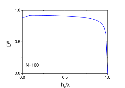
Figure 1: (Color online) $D^{H}$ of the ground state for $\gamma=1$ and $\lambda>0$ in LMG model.

As for $\lambda<0$, the minimal value of $E_{n}$ appears when $n=-\left[\tfrac{h_{z}}{|\lambda|}\tfrac{N}{2}\right]$. Then the ground state is $|N/2,N/2\rangle$ for $h_{z}>0$ and $|N/2,-N/2\rangle$ for $h_{z}<0$ in angular moment picture, which are Dicke states $|N,N\rangle_{\text{Dicke}}$ and $|N,0\rangle_{\text{Dicke}}$ respectively. Thus $D^{H}=0$.

-$\gamma\in[0,1)$- The ground state is cui06

$$|g\rangle = \frac{1}{c}\sum_{n=0}^{[N/2]}(-1)^{n}\sqrt{\tfrac{(2n-1)!!}{2n!!}}\tanh^{n}x|N,N-2n\rangle_{\text{Dicke}}$$

$$c^{2} = \sum_{n=0}^{[N/2]}(-1)^{n}\tfrac{(2n-1)!!}{2n!!}\tanh^{2n}x,$$ (79)

in which

$$\tanh 2x=\begin{cases}-\frac{1-\gamma}{2h_{z}-1-\gamma},&h_{z}>1\\ -\frac{h_{z}^{2}-\gamma}{2-h_{z}^{2}-\gamma},&0\leq h_{z}<1\end{cases}.$$ (80)

for $\lambda>0$ and

$$\tanh 2x=\frac{1-\gamma}{1+\gamma+2|h_{z}|}.$$ (81)

for $\lambda<0$.

In this case $\sigma$ has the same form as Eq.(V.1). In Fig.2, $D^{H}$ is plotted, in which the critical points can be identified, $h_{z}/\lambda=1$ for $\lambda>0$ and $h_{z}/\lambda=0$ for $\lambda<0$.

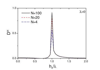
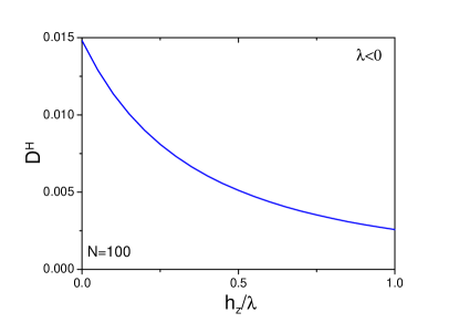
Figure 2: (Color online) $D^{H}$ of the ground state for $\gamma=1/2$ in LMG model.

A generalization of LMG is the so-called uniaxial model,

$$H=-\frac{1}{N}S^{2}_{x}-h_{x}S_{x}-h_{z}S_{z}.$$ (82)

The ground state has the same form to Eq.(V.1) with $\tanh 2x=\frac{2\Gamma(\lambda_{0})}{\Delta(\lambda_{0})}$, in which

$$\Gamma(\lambda_{0}) = -\frac{1-5\lambda_{0}^{2}}{4}+h_{x}\frac{\lambda_{0}(2-\lambda_{0}^{2})}{8(1-\lambda_{0}^{2})^{3/2}}$$

$$\Delta(\lambda_{0}) = h_{z}-\frac{1-7\lambda_{0}^{2}}{2}+h_{x}\frac{\lambda_{0}(4-3\lambda_{0}^{2})}{4(1-\lambda_{0}^{2})^{3/2}},$$ (83)

and $\lambda_{0}$ is determined by the equation

$$\lambda_{0}h_{z}-\frac{h_{x}(1-2\lambda_{0}^{2})}{2\sqrt{1-\lambda_{0}^{2}}}-\lambda_{0}(1-2\lambda_{0}^{2})=0.$$ (84)

There are two critical points, $h_{x}=0$ for $h_{z}=1$, which corresponds to a second order quantum phase transition and $h_{x}=0$ for $0<h_{z}<1$, a first order one. As shown in Fig. 3, $D^{H}$ can unambiguously manifest the appearance of critical points.

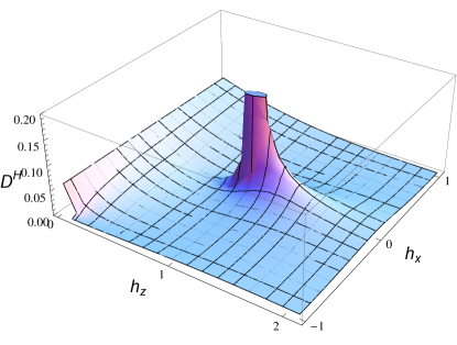
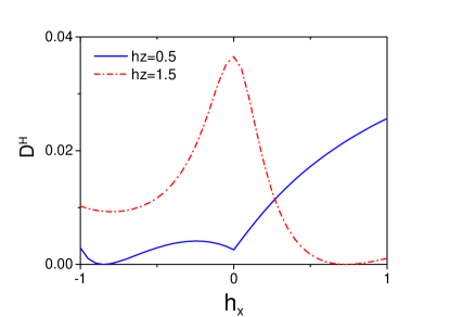
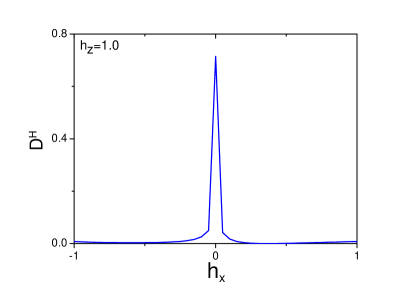
Figure 3: (Color online) $D^{H}$ of the ground state for uniaxial model when $N=20$.

V.2 Dicke model

Dicke model dicke is related to many fundamental issues in quantum optics, quantum mechanics and condensed matter physics, such as the coherent spontaneous radiationhh73 , the dissipation of quantum system leggett87 , quantum chaoshakee and atomic self-organization in a cavitybgbe09 . The multipartite entanglement in Dicke model has also been discussed multi-entanglement . The Hamiltonian for single-model Dicke model reads

$$H = \omega a^{\dagger}a+\frac{\omega_{0}}{2}\sum_{i=1}^{N}\sigma_{i}^{z}+\frac{\lambda}{\sqrt{N}}\sum_{i=1}^{N}(\sigma^{+}_{i}+\sigma^{-}_{i})(a^{\dagger}+a)$$ (85)

$$= \omega_{0}J_{z}+\omega a^{\dagger}a+\frac{\lambda}{\sqrt{N}}(a^{\dagger}+a)(J_{+}+J_{-}),$$

where $J_{z}=\sum_{i=1}^{N}\sigma_{i}^{z}/2$ and $J_{\pm}=\sum_{i=1}^{N}\sigma_{i}^{\pm}$ are the collective angular momentum operators. There are two distinct phases for ground state, normal phase and superradiant phase, separated by critical point $\lambda_{c}=\sqrt{\omega\omega_{0}}/2$.

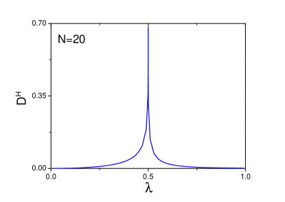
Figure 4: (Color online) $D^{H}$ of the ground state for Dicke model when $N=20$, in which we has set $\omega=\omega_{0}=1$ and the critical point $\lambda_{c}=0.5$.

By the method in Ref. eb03 , the reduce density operator of atom system for the ground state can be obtained analytically, which has the form

$$\rho=\sum_{k}\lambda_{k}|k\rangle\langle k|,$$ (86)

in which $|k\rangle=\sum_{n_{k}=0}^{N}C_{n_{k}}|N,n_{k}\rangle_{\text{Dicke}}$. It is obvious that $\rho$ is invariant under permutation. Then $\sigma$ is Eq. (V.1), and $D^{H}$ can be evaluated by numerical way, as shown in Fig. 4. Obviously it clearly marks the appearance of quantum phase transition.

VI Multilevel cases

The conjectures in this article can be generalized directly into multilevel case. In this section, we try to show the validity in comparison with two exactly solved examples in Ref. chang13 .

Example 1. $(m\times m)$-dimensional Werner state

$$\omega^{ab}=\tfrac{m-x}{m^{3}-m}\mathbf{I}^{ab}+\tfrac{mx-1}{m^{3}-m}F,$$ (87)

in which $x\in[-1,1]$ and $F=\sum_{k,l=1}^{m}|kl\rangle\langle lk|$. In matrix, $\omega^{ab}$ is the direct sum of the following sub-matrices

$$\omega_{1}^{ab} = \tfrac{1+x}{m^{2}+m}\sum_{k=1}^{m}|kk\rangle\langle kk|;$$

$$\omega_{2}^{ab} = \sum_{k\neq l}\omega_{kl}^{ab},$$ (88)

in which

$$\omega_{kl}^{ab} = \tfrac{m-x}{m^{3}-m}\left(|kl\rangle\langle kl|+|lk\rangle\langle lk|\right)$$ (89)

$$+\tfrac{mx-1}{m^{3}-m}\left(|kl\rangle\langle lk|+|lk\rangle\langle kl|\right).$$

Thus $\omega^{ab}$ is actually ”X” form, defined in Eq. (28).

It is easy to find

$$\sqrt{\omega^{ab}} = \sqrt{\tfrac{1+x}{m^{2}+m}}\sum_{k=1}^{m}|kk\rangle\langle kk|+\sqrt{\tfrac{1+x}{m^{2}+m}}\sum_{k\neq l}|1_{kl}\rangle\langle 1_{kl}|$$ (90)

$$+\sqrt{\tfrac{1-x}{m^{2}-m}}\sum_{k\neq l}|0_{kl}\rangle\langle 0_{kl}|,$$

in which $|1_{kl}\rangle=\tfrac{1}{\sqrt{2}}(|kl\rangle+|lk\rangle)$ and $|0_{kl}\rangle=\tfrac{1}{\sqrt{2}}(|kl\rangle-|lk\rangle)$. By Conjecture 2, the nearest neighbor $\sigma$ is

$$\sigma=\sum_{k}p_{k}|kk\rangle\langle kk|+\sum_{k\neq l}p_{kl}|kl\rangle\langle kl|,$$ (91)

in which $p_{k}$ and $p_{kl}$ is determined by Eq. (11). Thus by calculations,

$$\max\text{Tr}\left[\sqrt{\omega^{ab}}\sqrt{\sigma}\right]$$ (92)

$$= \left\{m\tfrac{1+x}{m+1}+\tfrac{m^{2}-m}{4}\left[\sqrt{\tfrac{1+x}{m^{2}+m}}\ +\sqrt{\tfrac{1-x}{m^{2}-m}}\ \right]^{2}\right\}^{1/2}$$

Thus one has

$$D^{H}(\omega^{ab})=1-\frac{1}{\sqrt{2}}\left[\frac{2+m+x}{m+1}+\sqrt{\frac{m-1}{m+1}}\sqrt{1-x^{2}}\right]^{1/2}.$$ (93)

Compared with the Eq. (15) in Ref. chang13

$$D_{H}(\omega^{ab})=1-\frac{1}{2}\left[\frac{2+m+x}{m+1}+\sqrt{\frac{m-1}{m+1}}\sqrt{1-x^{2}}\right],$$ (94)

it is not difficult to find that the two results are compatible and $D^{H}(\omega^{ab})<D_{H}(\omega^{ab})$.

Example 2. $(m\times m)$-dimensional isotropic state

$$\varsigma^{ab}=\frac{1-x}{m^{2}-1}\mathbf{I}^{ab}+\frac{mx^{2}-1}{m^{2}-1}|\Psi^{+}\rangle\langle\Psi^{+}|,$$ (95)

in which $|\Psi^{+}\rangle=\tfrac{1}{\sqrt{m}}\sum_{k=1}^{m}|kk\rangle$. In matrix, $\varsigma^{ab}$ is direct sum of two submatrices, spanned by the local orthonormal bases $\{|kk\rangle,k=1,2,\cdots,m\}$ and $\{|kl\rangle,k\neq l\}$ respectively. However $\varsigma^{ab}$ does not show a ”X” form so that an independent discussion is needed.

It should be pointed out that because of the isotropic feature, $|\Psi^{+}\rangle$ is already in the Schmidt decomposition. The other orthonormal states in the subspace spanned by $\{|kk\rangle,k=1,2,\cdots,m\}$ is written as

$$|\Psi_{n}^{+}\rangle=\tfrac{1}{\sqrt{m}}\sum_{k=1}^{m}e^{i2n\pi\tfrac{k-1}{m}}|kk\rangle,n=1,2,\cdots,(m-1).$$ (96)

Thus

$$\sqrt{\varsigma^{ab}} = \sqrt{x}|\Psi^{+}\rangle\langle\Psi^{+}|+\sqrt{\frac{1-x}{m^{2}-1}}\sum_{n=1}^{m-1}|\Psi_{n}^{+}\rangle\langle\Psi_{n}^{+}|$$ (97)

$$+\sqrt{\frac{1-x}{m^{2}-1}}\sum_{k\neq l}|kl\rangle\langle kl|.$$

Consequently the nearest neighbor $\sigma$ should be the following form

$$\sigma=\sum_{k=1}^{m}p_{k}|kk\rangle\langle kk|+\sum_{k\neq l}p_{kl}|kl\rangle\langle kl|,$$ (98)

in which $p_{k}$ and $p_{kl}$ can be decided by Eq. (11).

By calculation one can obtain

$$\max\text{Tr}\left[\sqrt{\varsigma^{ab}}\sqrt{\sigma}\right]$$ (99)

$$= \sqrt{m\left[\tfrac{\sqrt{x}}{m}+\tfrac{m-1}{m}\sqrt{\tfrac{1-x}{m^{2}-1}}\right]^{2}+(m^{2}-m)\tfrac{1-x}{m^{2}-1}}.$$

Thus

$$D^{H}(\varsigma^{ab})=1-\sqrt{\tfrac{(1-x)(m^{2}-1)+m}{m(m+1)}+\tfrac{2}{m}\sqrt{\tfrac{m-1}{m+1}}\sqrt{x(1-x)}},$$ (100)

which is obviously compatible with Eq. (17) in Ref. chang13

$$D_{H}(\varsigma^{ab})=1-\left\{\tfrac{(1-x)(m^{2}-1)+m}{m(m+1)}+\tfrac{2}{m}\sqrt{\tfrac{m-1}{m+1}}\sqrt{x(1-x)}\right\}.$$ (101)

In this section we demonstrate the generality and popularity of our conjectures by two examples. We also note that $D^{H}$ is always less than $D_{H}$, defined by Eq. (2) in Ref. chang13 .

VII Conclusion and Discussion

In conclusion, a generalization of the geometric measure of quantum discord is introduced in this article. Our definition can be generalized readily into multipartite case. Moreover since the adopted Hellinger distance and the uninvolved of local measurements, it does not suffered from the critiques raised recently in Refs. dakic ; pz ; gheorghiu14 . An important conclusin in this article is that in order to determine the optimal value of Eq. (1), it is necessary to find the Schmidt decomposition for the measured state. Then the optimal completely classical state $\sigma$ is a joint distribution of the corresponding Schmidt basis with the probability decided by Eqs. (8) and (11). In Section III we display the validity of the result by exactly solving several examples. Then two conjectures are presented. Up to our knowledge, it is the first general exact result for the geometric measure of quantum discord. For multipartite states, the geometric discord can also be evaluated exactly if the state possesses the invariance under permutation or translation, as shown in Section IV. Furthermore it is pointed out in Conjecture 3 that the optimal $\sigma$ necessarily have the same invariance. In Section V we show by two models that our new definition can be used to mark the quantum phase transitions in many-body systems. A discussion of multilevel case is also presented in Section VI. Two examples are worked out exactly, which also are studied in Ref. chang13 . The fact that our results are compatible with that in Ref. chang13 unambiguously shows the validity and generality of our conjectures in this article.

Finally we provide a further discussion on our conclusion. As claimed in this article that the optimal $\sigma$ is determined by the Schmidt decomposition of bipartite state, It seems a natural hypothesis that one could found the generalized Schmidt decomposition for multipartite state based on the ”nearest” $\sigma$. Then a geometric understanding of Schmidt decomposition can be constructed by this way, which is inevitably interesting, e.g., in the measure of quantum correlation. Although this approaching is instructive, there are some problems to answer at first. First as for pure bipartite state, the Schmidt decomposition can be used to quantify the quantum entanglement in the state. However it is unclear that this feature is preserved or not when generalized into multipartite. Second as for mixed state, what the meaning of Schmidt decomposition is. We do not know how to understand this point by now. However it is still an interesting way to found the geometric understanding of quantum correlation.

References

- (1) L. Herderson, and V. Vedral. J. Phys. A: Math. and Gen. 34, 6899 (2001); H. Olliver and W. H. Zurek, Phys. Rev. Lett. 88, 017901 (2001);
- (2) A. Datta, A. Shaji, and C.M. Caves, Phys. Rev. Lett. 100, 050502 (2008).
- (3) V. Giovannetti, S. Lloyd, and L. Maccone, Science, 306, 1330 (2004).
- (4) K. Modi, A. Brodutch, H. Cable, T. Paterek, and V. Vedral, Rev. Mod. Phys. 84, 1655 (2012); Special issue ”Classical Vs Quantum correlations in composite systems” edited by L. Amico, S. Bose, V. Korepin and V. Vedral, Int. J. Mod. Phys. B 27, Nos.1 and 3, 1345011-1345055 (2013).
- (5) Shunlong Luo, Phys. Rev. A 77, 042303 (2008).
- (6) M. Ali, A.P.R. Rau, and G. Alber, Phys. Rev. A 81, 042105 (2010).
- (7) Yicheng Huang, Phys. Rev. A 88, 014302 (2013)
- (8) Yicheng Huang, New J. Phys. 16, 033027 (2014).
- (9) B. Dakić, V. Vedral, and C̆. Brukner, Phys. Rev. Lett. 105, 190502 (2010).
- (10) Shunlong Luo and Shuangshuang Fu, Phys. Rev. A 82, 034302 (2010).
- (11) M. Ozawa, Phys. Lett. A 268, 158-160 (2000); X. Wang and S.G. Schirmer, Phys. Rev. A 79, 052326 (2009); M. Piani, Phys. Rev. A 86, 034101 (2012).
- (12) V. Gheorghiu, M C. de Oliveira, and B. C. Sanders, Phys. Rev. Lett. 115, 030403 (2015);
- (13) T. Tufarelli, T. MacLean, D. Girolami, R. vasile, and G. Adesso, J. Phys. A: Math. Theor. 46, 275308 (2013).
- (14) F.M. Paula,Thiago R. de Oliveira, and M.S. Sarandy, Phys. Rev. A 87, 064101 (2013); S.J. Akhtarshenas, H. Mohammadi, S. Karimi, and Z. Azmi, arXiv: 1303.5570; F. Ciccarello, T. Tufarelli, and V. Giovannetti, New J. Phys 16, 0103038 (2014).
- (15) D. Spehner and M. Orszag, New. J. Phys, 15, 103001 (2013); ibid, J. Phys. A: Math. Theor. 47, 035302 (2014).
- (16) Lina Chang and Shunlong Luo, Phys. Rev. A 87, 062303 (2013).
- (17) Shunlong Luo and Qiang Zhang, Phys. Rev. A 69, 032106 (2004).
- (18) J. Dajka, J. Łucaka and P. Hänggi, Phys. Rev. A 84, 032120 (2011).
- (19) G.L. Giorgi, B. Bellomo, F. Galve, and R. Zambrini, Phys. Rev. Lett. 107, 190501 (2011); I. Chakrabarty, P. Agrawal, and A.K. Pati. Eur. Phys. J. D 65, 605-612 (2011).
- (20) Y.K. Bai, N. Zhao, M.Y. Ye, and Z.D. Wang, Phys. Rev. A 88, 012123 (2013).
- (21) C.C. Rulli and M.S. Sarandy, Phys. Rev. A 84, 042109 (2011); M. Okrasa and Z. Walczak, EuroPhys. Lett. 96, 60003 (2011).
- (22) Jianwei Xu, J. Phys. A: Math. Theor. 45, 405304 (2012).
- (23) N. Li and S. Luo, Phys. Rev. A 78, 024303 (2008).
- (24) K. Modi, T. Paterek, W. Son, V. Vedral, and M. Williamson, Phys. Rev. Lett. 104, 080501 (2010).
- (25) H. T. Cui, D. Yuan and J.L. Tian, Phys. Rev. A 82, 062116 (2010); H.T. Cui, J.L. Tian, C.M. Wang and Y. C. Chen, Eur. Phys. J. D 67, 154 (2013).
- (26) H. J. Lipkin, N. Meshkov, A. J. Glick, Nucl. Phys. 62, 188 (1965); 62, 199 (1965); 62, 211(1965).
- (27) R.H. Dicke, Phys. Rev. 93, 99(1954).
- (28) J. Vidal. G. Palacios, R. Mosseri, Phys. Rev. A, 69, 022107(2004); J. Vidal, Phys. Rev. A 73, 062318(2006).
- (29) R. Botet, R. Jullien. P. Pfeuty, Phys. Rev. Lett. 49, 478 (1982); R. Botet, R. Jullien, Phys. Rev. B 28, 3955 (1983).
- (30) H.T. Cui, K. Li, X.X. Yi, Phys. Lett. A 360, 243(2006).
- (31) K. Hepp and E.H. Lieb, Ann. Phys. (N.Y.) 76, 360(1973); Y.K. Wang and F.T. Hioe, Phys. Rev. A 7, 831(1973);
- (32) A.J. Leggett, S. Chakravarty, A.T. Dorsey, M.P.A. Fisher, A. Garg, W. Zwerger, Rev. Mod. Phys. 59, 1(1987).
- (33) F. Haake, Quantum Signatures of Chaos(Springer, Berlin, Heidelberg, 2001).
- (34) K. Baumann, C. Guerlin, F. Brennecke, and T. Esslinger, Nature 464, 1301 (2010).
- (35) N. Lamber, C. Emary, and T. Brandes, Phys. Rev. Lett. 92, 073602(2004); Phys. Rev. A 71, 053804(2005); J. Vidal, S. Dusuel, T. Barthel, J. Stat. Mech. P01015(2007); S. Campbell, M. S. Tame, and M. Paternostro, New J. Phys. 11, 073039 (2009); H. T. Cui, Phys. Rev. A 81, 042112 (2010).
- (36) C. Emary and T. Brandes, Phys. Rev. E 67, 066203 (2003).