Symmetry and Dirac points in graphene spectrum

Abstract.

Existence and stability of Dirac points in the dispersion relation of operators periodic with respect to the hexagonal lattice is investigated for different sets of additional symmetries. The following symmetries are considered: rotation by $2\pi/3$ and inversion, rotation by $2\pi/3$ and horizontal reflection, inversion or reflection with weakly broken rotation symmetry, and the case where no Dirac points arise: rotation by $2\pi/3$ and vertical reflection.

All proofs are based on symmetry considerations. In particular, existence of degeneracies in the spectrum is deduced from the (co)representation of the relevant symmetry group. The conical shape of the dispersion relation is obtained from its invariance under rotation by $2\pi/3$. Persistence of conical points when the rotation symmetry is weakly broken is proved using a geometric phase in one case and parity of the eigenfunctions in the other.

1. Introduction

Many interesting physical properties of graphene [32, 9, 24, 16], are consequences of presence of special conical points in the dispersion relation, where its different sheets touch to form a conical singularity. These points are often referred to as Dirac points or as diabilical points.

Most mathematical analyses of the dispersion relation of graphene are performed in physics literature in the tight-binding approximation, starting from the work of Wallace [40] and Slonczewski and Weiss [37]. This is equivalent to modeling the material as a discrete graph with vertices at the carbon molecules’ locations and with edges indicating chemical bonds. A richer mathematical model for graphene was considered by Kuchment and Post in [27], who studied honeycomb quantum graphs with even potential on edges.

The Schrödinger operator $H_{\varepsilon}=-\Delta+\varepsilon q(\vec{x})$ in $\mathbb{R}^{2}$ with the real-valued potential $q(\vec{x})$ that has honeycomb symmetry was considered by Grushin [20]. A condition for a multiple eigenvalue to be a conical point was established and checked in the perturbative regime of a weak potential (small $\varepsilon$). The multiplicity two of the eigenvalue was proved from the symmetry point of view, an approach that we fully develop here.

The case of potential of arbitrary strength was studied by Fefferman and Weinstein [15] (see also [14] for further results). The results of [15] can be schematically broken into three parts: (a) establish that the dispersion relation has a double degeneracy at certain known values of quasi-momenta; (b) establish that for almost all $\varepsilon$ the dispersion relation is conical in the vicinity of the degeneracy; (c) prove that the conical singularities survive under weak perturbation which destroys some of the symmetries of the potential (namely, the rotational symmetry). These results are contained in [15, Thms 5.1(1), 4.1 and 9.1] with proofs which are rather technical.

The purpose of this article is to make explicit the role of symmetry in existence and stability of Dirac points and to give proofs that are at the same time simpler and more general. Our methods apply to many different settings: graphs (discrete or quantum) and Schrödinger and Dirac operators on $\mathbb{R}^{2}$. We use Schrödinger operator as our primary focus, and give numerical examples based on discrete graphs. We also consider the effect of different symmetries, substituting inversion symmetry, usually assumed in the literature, with horizontal reflection symmetry (the results are analogous or stronger, as explained below).

We will now briefly review our results and the methods employed. The Schrödinger operator is assumed to be shift-invariant with respect to the hexagonal lattice. We also consider the following symmetries (see Fig. 1 for an illustration): rotation by $2\pi/3$ (henceforth, “rotation”), inversion (reflection with respect to the point $(0,0)$), horizontal reflection and, to a lesser extent, vertical reflection. We remark that horizontal and vertical reflections are substantially different because the hexagonal lattice is not invariant with respect to rotation by $\pi/2$. We study the question of existence and stability of Dirac points when the operator has various subsets of the above symmetries.

We show that existence of the degeneracy is a direct consequence of symmetries of the operator. The natural tool for studying this is, of course, the representation theory. It is well known that existence of a two- (or higher-) dimensional irreducible representation suggests that some eigenvalues will be degenerate. However, rotation combined with inversion — the most usual choice of symmetries [20, 15] — is an abelian group, whose irreps are all one-dimensional. The resolution of this question lies in the fact that the relevant symmetry is the inversion combined with complex conjugation and one should look at representations combining unitary and antiunitary operators, the so-called corepresentations introduced and fully classified by Wigner [43, Chap. 26].

To prove the existence of the degeneracy in the spectrum (Lemma 4.3) we identify the 2-dimensional (co)representation responsible for it and describe the subspace of the Hilbert space that carries this representation. We also relate our results to the proofs of isospectrality, in particular the isospectrality condition of Band–Parzanchevski–Ben-Shach [5, 33].

The conical nature of the dispersion relation is known to be generic (see, for example, [2, Appendix 10]); to prove this in a particular case one uses perturbation theory, as done in [20] and, implicitly, in [15]. Again, we seek to make the effect of symmetry most explicit here. This is done on two levels. First, in Lemma 2.1 and Lemma 3.1 we show that the dispersion relation also has rotational symmetry and thus, by Hilbert-Weyl theory of invariant functions, is restricted to be a circular cone (which could be degenerate) plus higher order terms. Then, in Lemma 5.2, we show that the symmetries also enforce certain relations on the first order terms of the perturbative expansion of the operator, which restricts the possible form of the terms. In spirit, this conclusion parallels the Hilbert-Weyl theory, but is more powerful: for example, it allows us to conclude that at quasi-momentum $\vec{0}$, where we discover persistent degeneracies with only the rotational symmetry, the dispersion relation is locally flat.

Part (c) of the above classification, the survival of the Dirac points when a weak perturbation breaks the rotational symmetry, can be established by perturbation theory and implicit function theorem, as done in [15]. However, such resilience of singularities indicates that there are topological obstacles to their disappearance [30, 29, 31]. The method familiar to physicists is to use the Berry phase [6, 36], which works when the operator has inversion symmetry (Section 7.1). Interestingly, when instead of inversion symmetry we have horizontal reflection symmetry, Berry phase is not restricted to the integer multiples of $\pi$ and the topological obstacle has a different nature. The survival of the Dirac cone is shown to be a consequence of the structure of representation of the reflection symmetry (Section 7.2), which combines eigenfunctions of different parities at the degeneracy point. As a consequence of our proof we conclude that the perturbed cone, although shifted from the corner of the Brillouin zone, remains on a certain explicitly defined line. In particular, this restricts the location of points in the Brillouin zone where Dirac cones can be destroyed by merging with their symmetric counterparts. Naturally, this effect is also present when there is horizontal reflection symmetry in addition to the inversion symmetry. We remark that experimentally created potentials usually possess the reflection symmetry, [4, 38].

In connection with the survival of the Dirac points, we would like to mention the complementary result of by Colin de Verdière in [10], who considered the Schrödinger operator $H_{\varepsilon}=-\Delta+\varepsilon q(\vec{x})$ with $q(\vec{x})$ periodic, real and inversion-symmetric, but not $2\pi/3$-rotation invariant. In this case, for small $\varepsilon$, there are also conical singularities of the dispersion in the vicinity of the same special quasi-momenta. The proof uses the transversality condition of von Neumann–Wigner [39] and Arnold [1]. The method of [10] or, on a more basic level, the implicit function theorem, could also be used to prove our results, but we feel that the Berry phase technique is both beautiful and relatively unknown in the mathematics literature and thus deserves an appearance.

To summarize, in addition to providing simpler and shorter symmetry-based proofs to existing results, we discover some previously unknown consequences. In particular, we consider the case of rotational symmetry coupled with horizontal reflection symmetry; in this case, when the rotational symmetry is weakly destroyed, the conical points travel on a special line. We observe degeneracies at quasi-momentum $\vec{0}$ in presence of rotational symmetry only; the dispersion relation at this point is shown to be locally flat. Finally, we explain why the coupling of rotation and vertical reflection does not, in general, lead to the appearance of Dirac points. The tools developed in this article would be easily extensible to other lattice structures [11] and graphene superlattices [44, 34].

1.1. Symmetries

The periodicity lattice of the operators that we consider is the 2-dimensional hexagonal lattice $\Gamma$ with the basis vectors

(1) $$\vec{a_{1}}=\begin{pmatrix}\sqrt{3}/2\\ 1/2\end{pmatrix},\qquad\vec{a_{2}}=\begin{pmatrix}\sqrt{3}/{2}\\ -1/2\end{pmatrix},$$

see Fig. 1(a). The operator considered will always be assumed to be invariant with respect to the shifts by this lattice.

In addition to the shifts, the lattice $\Gamma$ has several other symmetries. We now describe some of them as operators acting on functions on $\mathbb{R}^{2}$ (or on a graph embedded into $\mathbb{R}^{2}$).

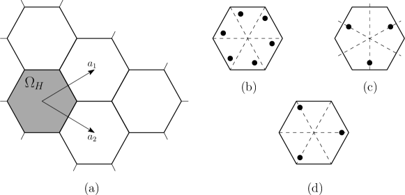
Figure 1. Hexagonal lattice (a) and examples of fundamental domains with symmetry $R$ and, additionally, (b) inversion symmetry $V$, (c) horizontal reflection symmetry $F$ and (d) vertical reflection symmetry $F_{V}$. Note that we do not expect conical points in operators with symmetries $R$ and $F_{V}$, see section 4.1.4.

• Rotation $R$ by $2\pi/3$ in the positive (counter-clockwise) direction:

  $$R:\psi(x_{1},x_{2})\mapsto\psi\left(-\frac{1}{2}x_{1}+\frac{\sqrt{3}}{2}x_{2},-\frac{\sqrt{3}}{2}x_{1}-\frac{1}{2}x_{2}\right)=\psi\left(M_{R}\vec{x}\right).$$

• Inversion $V$:

  $$V:\psi(x_{1},x_{2})\mapsto\psi(-x_{1},-x_{2}).$$

• Horizontal reflection $F$:

  $$F:\psi(x_{1},x_{2})\mapsto\psi(-x_{1},x_{2}).$$

Note that $R$ and $V$ together form the abelian group of rotations by multiples of $\pi/3$.

We denote by $C$ the antiunitary operation of taking complex conjugation (or “time-reversal” in physics terminology),

(2) $$C:\psi(x_{1},x_{2})\mapsto\overline{\psi(x_{1},x_{2})}.$$

In what follows, we will assume our operator has symmetries generated by a subset of the following: complex conjugation $C$, rotation $R$, reflection $F$, conjugate inversion $\overline{V}=VC$.

As the base operator (i.e. before we apply Floquet-Bloch analysis) we will always take an operator with real coefficients, thus it will be symmetric with respect to complex conjugation. As it turns out, an important role is played by the product of inversion and complex conjugation, known as the $\mathcal{PT}$ (parity-time) transformation:

Finally, we will also consider the vertical reflection symmetry:

• Vertical reflection $F_{V}$:

  $$F_{V}:\psi(x_{1},x_{2})\mapsto\psi(x_{1},-x_{2}).$$

Its effect is not the same as that of the horizontal reflection $F$ because the two symmetries are aligned differently with respect to the lattice $\Gamma$. In fact, in contrast to $F$, the presence of $F_{V}$ (in addition to symmetry $R$) does not generally lead to the appearance of conical points in the dispersion relation. This negative result is also important to understand; we explain it in section 4.1.4.

In Fig. 1(b-d) we show the fundamental domain of the lattice with defects that have symmetry $R$ in addition to $V$, $F$ or $F_{V}$, correspondingly.

1.2. Operators

As our primary motivational example we use the two-dimensional Schrödinger operator

(3) $$H=-\Delta+q(\vec{x}),\qquad\vec{x}\in\mathbb{R}^{2},$$

with the real-valued potential $q(\vec{x})$ assumed to be bounded and periodic with respect to the lattice $\Gamma$. For general properties of the dispersion relation of such operators we refer the reader to [3, 25, 26].

To generate simple numerical examples we use discrete Schrödinger operators with potentials crafted to break or retain some of the symmetries listed above. More precisely, denote by $G=(V,E)$ an infinite graph embedded in $\mathbb{R}^{2}$, with vertex set $V$ and edge set $E$. The embedding is realized by the mapping $\operatorname{loc}:V\to\mathbb{R}^{2}$ which gives the location in $\mathbb{R}^{2}$ of the given vertex. A transformation $T:\mathbb{R}^{2}\to\mathbb{R}^{2}$ preserves the graph structure if $u_{1},u_{2}\in V$ implies existence of $u_{1}^{\prime},u_{2}^{\prime}\in V$ such that $T\operatorname{loc}(u_{j})=\operatorname{loc}(u_{j}^{\prime})$ and $u_{1}^{\prime},u_{2}^{\prime}$ are connected by an edge if and only if $u_{1},u_{2}$ are connected.

The graph is $\Gamma$-periodic if the graph structure is preserved by the shifts defining the lattice. A graph with space symmetry $S$ is defined analogously.

The Schrödinger operator is defined on the functions from $\ell^{2}(\mathbb{C}^{V})$ by

(4) $$(Hf)_{v}=\sum_{(v,u)\in E}m_{v,u}(f_{v}-f_{u})+q_{v}f_{v},$$

where the sum is over all vertices $u$ adjacent to $v$, $m_{v,u}>0$ are weights associated to edges (often, they are taken inversely proportional to edge length) and $q:V\to\mathbb{R}$ is the discrete potential. In our examples, the graph structure will be compatible with all symmetries of the lattice $\Gamma$, while $m$ and $q$ will be breaking some of the point symmetries (however, they will always be periodic). The simplest $\Gamma$-periodic graph is shown in Fig. 8(a). This is the graph arising as the tight-binding approximation of graphene.

Note that the discrete Schrödinger operator on graphs with more than two atoms per unit cell is not a mere mathematical curiosity since it arises in studying the twisted graphene and graphene in a periodic potential (superlattice); see [28, 44, 41] and references therein.

Remark 1.1.

We will always assume that $H$ is time-reversal (TR) invariant, or, in other words, satisfies

$$CHC=H,$$

with $C$ the complex conjugation from (2). In particular, in the case (3), this means that $q$ is real-valued, while in the case (4) this means that both $q$ and $m$ are real-valued.

1.3. Floquet-Bloch reduction

Floquet theory can be thought of as a version of Fourier expansion, mapping the spectral problem on a non-compact manifold into a continuous sum of spectral problems on a compact manifold. The compact spectral problems are parametrized by the representations of the abelian group of periods (shifts).

Denote by $\mathcal{X}(\vec{k})$, $\vec{k}=(k_{1},k_{2})\in\mathbb{T}^{2}:=[0,2\pi)^{2}$ the space of Bloch functions, i.e. locally $L^{2}$ functions satisfying

(5) $$\psi(\vec{x}+n_{1}\vec{a_{1}}+n_{2}\vec{a_{2}})=e^{i(n_{1}k_{1}+n_{2}k_{2})}\psi(x),\qquad n_{1},n_{2}\in\mathbb{Z}.$$

For functions $\psi\in\mathcal{X}(\vec{k})$ which also belong to the domain of $H$ it can be immediately seen that

$$(H\psi)(x+n_{1}\vec{a_{1}}+n_{2}\vec{a_{2}})=e^{i(n_{1}k_{1}+n_{2}k_{2})}H\psi(x),$$

i.e. the space $\mathcal{X}(\vec{k})$ is invariant under $H$. By $H(\vec{k})$ we will denote the restriction of the operator $H$ to the space $\mathcal{X}(\vec{k})$. Its domain is $\mathcal{X}^{2}(\vec{k})$, the dense subspace of $\mathcal{X}(\vec{k})$ consisting of functions that locally belong to $L^{2}$ together with their derivatives up to the second order.

Figure 2. Floquet-Bloch reduction on the plane with hexagonal lattice generated by $\vec{a_{1}}$ and $\vec{a_{2}}$.

Choosing a fundamental domain of the action of the group of periods, we can reduce the problem to the fundamental domain with quasi-periodic boundary conditions. The result of the Floquet-Bloch reduction is shown in Fig. 2. In Fig. 1(a), the lattice generating vectors $\vec{a_{1}}$ and $\vec{a_{2}}$ were shown together with a convenient choice of the fundamental region (shaded) and its four translations, by $\vec{a}_{1}$, $\vec{a}_{2}$, $\vec{a}_{1}-\vec{a}_{2}$ and $\vec{a}_{1}+\vec{a}_{2}$. We will denote this choice of the fundamental domain by $\Omega_{H}$. The values of a Bloch function in surrounding regions, according to equation (5), are indicated in Fig. 2(a); we use the notation

(6) $$\omega_{j}=e^{ik_{j}},\qquad j=1,\,2.$$

The continuity of the function and its derivative across the boundaries of copies of the fundamental region impose boundary conditions shown schematically in Fig. 2(b). They should be understood as follows: taking the bottom and top boundaries as an example, and parametrizing them left to right, the conditions read

$$\psi\big{|}_{\mathrm{top}}=\overline{\omega_{2}}\omega_{1}\psi\big{|}_{\mathrm{bottom}},\qquad-\partial_{\vec{n}}\psi\big{|}_{\mathrm{top}}=\overline{\omega_{2}}\omega_{1}\partial_{\vec{n}}\psi\big{|}_{\mathrm{bottom}},$$

where the normal derivative is taken in the outward direction (this causes the minus sign to appear). We stress that in Fig. 2(c) we use letters $f$, $g$ and $h$ as placeholder labels, connecting the values of the function and its derivative on similarly labeled sides.

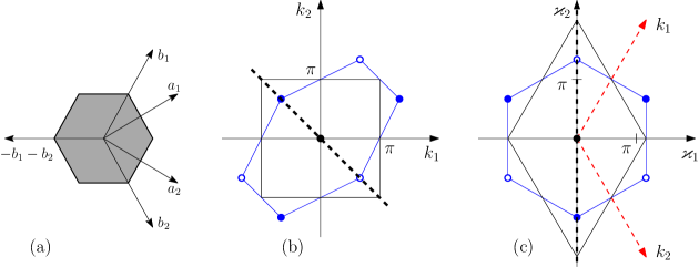
Figure 3. The dual basis (a) to the vectors $\vec{a_{1}}$ and $\vec{a_{2}}$ and two choices of the Brillouin zone in terms of (b) coordinates $k_{1},k_{2}$ (drawn as if they were Cartesian) and (c) coordinates $\varkappa_{1},\varkappa_{2}$ (which are Cartesian); part (c) also shows the correct position for the axes $k_{1}$ and $k_{2}$. The axis of symmetry of the operator $\hat{F}$ is shown in dashed line (the equation $k_{1}=-k_{2}$). Fixed points of the operator $\hat{R}$ are shown by circles (different fill styles correspond to different points of symmetry).

To represent the exponent of the Bloch phase $n_{1}k_{1}+n_{2}k_{2}$ as a scalar product, we introduce the vectors

(7) $$\vec{b_{1}}=\left(\frac{1}{\sqrt{3}},1\right)^{T},\qquad\vec{b_{2}}=\left(\frac{1}{\sqrt{3}},-1\right)^{T},$$

see Fig. 3(a). Then

(8) $$\left.\vec{b}_{i}\right.^{T}\cdot\vec{a}_{j}=\delta_{i,j}.$$

The vectors $\vec{b}_{1}$, $\vec{b}_{2}$ define a lattice which is known as the dual lattice. For a hexagonal lattice, the dual lattice is also hexagonal. The lattice spanned by the vectors $2\pi\vec{b}_{1}$, $2\pi\vec{b}_{2}$ will be denoted $\Gamma^{*}$.

Due to (8), one can write $n_{1}k_{1}+n_{2}k_{2}$ as the dot product

$$n_{1}k_{1}+n_{2}k_{2}=\big{(}k_{1}\vec{b_{1}}+k_{2}\vec{b_{2}}\big{)}\cdot\big{(}n_{1}\vec{a_{1}}+n_{2}\vec{a_{2}}\big{)}.$$

Let us comment on using coordinates $k_{1},k_{2}$ which are the coordinates with respect to the basis $\vec{b}_{1},\vec{b}_{2}$ versus the corresponding Cartesian coordinates $\varkappa_{1},\varkappa_{2}$ given by

(9) $$\vec{\varkappa}=\begin{pmatrix}\tfrac{1}{\sqrt{3}}&\tfrac{1}{\sqrt{3}}\\[3.0pt] 1&-1\end{pmatrix}\vec{k}=:B\vec{k}\quad\mbox{or, equivalently,}\quad\vec{k}=B^{-1}\vec{\varkappa}=\begin{pmatrix}\tfrac{\sqrt{3}}{2}&\tfrac{1}{2}\\[3.0pt] \tfrac{\sqrt{3}}{2}&-\tfrac{1}{2}\end{pmatrix}\vec{\varkappa}.$$

In Fig. 3(b) we show two choices of the Brillouin zone drawn in terms of coordinates $k_{1},k_{2}$ and coordinates $\varkappa_{1},\varkappa_{2}$. One arrives at the first picture if one uses $k_{1}$ and $k_{2}$ as parameters for the dispersion relation (which is natural) ranging from $-\pi$ to $\pi$ (black square) and then plots the result using $k_{1}$ and $k_{2}$ as Cartesian coordinates. The resulting plot of the dispersion relation will be skewed similarly to the blue hexagon in Fig. 3(b) (cf. Figures 5 and 6 of [27]). A more correct way of plotting is over a domain in Fig. 3(c), as it will highlight the symmetries of the result (see Figs. 4 and 5 and the explanations in the following section).

2. Formulation of results

For each value of the quasi-momentum $\vec{k}$, the operator $H(\vec{k})$ has discrete spectrum. Its eigenvalues as functions of $\vec{k}$ form what is known as the dispersion relation. Our results are concerned with the structure of the dispersion relation for the operators we described in Section 1.2. A typical example is shown in Fig. 4; it was computed for a discrete Laplacian described in detail in Example 4.5.

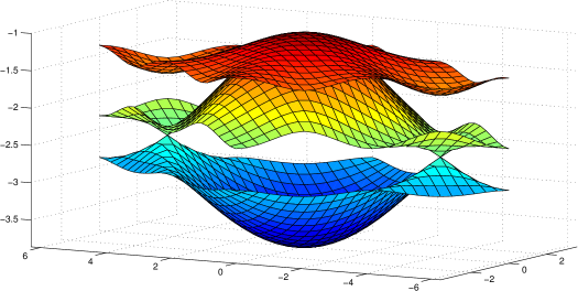
Figure 4. The lowest three bands of the dispersion relation of the graph from Example 4.5, which has reflection symmetry. The lower two bands touch conically at the points $\pm\vec{k}^{*}$. The Brillouin zone is parametrized by $\vec{\varkappa}$ coordinates.

In the figure, one can see two conical points where the lowest two sheets of the dispersion relation touch. In terms of $\vec{k}$ coordinates, they touch at $\pm\vec{k}^{*}$, where

$$\vec{k}^{*}=\left(\frac{2\pi}{3},-\frac{2\pi}{3}\right),\quad\mbox{or, correspondingly,}\quad\vec{\varkappa}^{*}=\left(0,\frac{4\pi}{3}\right).$$

The middle and the top sheets also touch, at the point $\vec{0}=(0,0)$; at the point of contact both surfaces are locally flat. We will show that these features are typical: conical singularities at the point $\vec{k}^{*}$ and flat contact at the point $\vec{0}$.

We start with formulating the following well-known result, summarizing the effects the different symmetries of $H$ have on the structure of the dispersion relation.

Lemma 2.1.

1. If the operator $H$ is $\Gamma$-periodic (i.e. invariant with respect to the shifts by the lattice $\Gamma$), then the dispersion relation $\lambda_{n}(\vec{\varkappa})$ is $\Gamma^{*}$-periodic, i.e. invariant with respect to the shifts

   (10) $$\vec{\varkappa}\mapsto\vec{\varkappa}+2\pi b_{1}\qquad\mbox{and}\qquad\vec{\varkappa}\mapsto\vec{\varkappa}+2\pi b_{2}.$$

2. If the operator $H$ is invariant with respect to complex conjugation $C$ or inversion $V$, then the dispersion relation $\lambda_{n}(\vec{\varkappa})$ is invariant with respect to the inversion $\varkappa\to-\varkappa$.

3. If the operator $H$ is invariant with respect to horizontal reflection $F$, then the dispersion relation $\lambda_{n}(\vec{\varkappa})$ is invariant with respect to the reflection $(\varkappa_{1},\varkappa_{2})\to(-\varkappa_{1},\varkappa_{2})$.

4. If the operator $H$ is invariant with respect to rotation $R$, then the dispersion relation $\lambda_{n}(\vec{\varkappa})$ is invariant with respect to rotation by $2\pi/3$ around the point $\vec{0}=(0,0)$.

   1. If, in addition to symmetry $R$, the operator $H$ is $\Gamma$-periodic, then the dispersion relation is also invariant with respect to rotation by $2\pi/3$ around the points $\pm\vec{\varkappa}^{*}:=\pm(0,4\pi/3)$.

   2. If, in addition to symmetry $R$, the operator $H$ has symmetry $V$ or $C$, the dispersion relation is invariant with respect to rotation by $\pi/3$ around the point $\vec{0}=(0,0)$.

For completeness, we provide the proof in Section 3.

Remark 2.2.

When $H$ is invariant with respect to complex conjugation, inversion symmetry of the operator does not result in any additional symmetries of the dispersion relation.

Example 2.3.

Figure 4 was produced for a $\Gamma$-periodic graph operator which has symmetries $R$, $C$ and $F$ (but not $V$). Its dispersion relation therefore has symmetry groups $D_{6}$ around the point $\vec{0}$, and $D_{3}$ around the points $\pm\vec{\varkappa}^{*}$ ($D_{3}$ and $D_{6}$ are the groups of symmetries of equilateral triangle and hexagon). This can be seen clearly if we plot the level curves of the dispersion surfaces, Fig. 5.

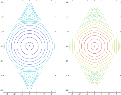
Figure 5. The contour plots of the two lowest bands from Fig. 4. Because of the symmetry of the operator (rotation, complex conjugation and reflection), the contours have the symmetry of an equilateral hexagon around $(0,0)$ and equilateral triangle around the points $\pm\vec{\varkappa}^{*}$.

Theorem 2.4.

Let the self-adjoint $\Gamma$-periodic operator $H$ be invariant under rotation $R$. Let $\vec{k}_{0}$ be one of the points $\vec{k}^{*}$, $-\vec{k}^{*}$ or $\vec{0}$. The space $\mathcal{X}(\vec{k}_{0})$ splits into the orthogonal sum

(11) $$\mathcal{X}(\vec{k}_{0})=\mathcal{X}_{0}(\vec{k}_{0})\oplus\mathcal{X}_{\perp}(\vec{k}_{0}),$$

where $\mathcal{X}_{0}(\vec{k}_{0})=\{\psi\in\mathcal{X}(\vec{k}_{0}):R\psi=\psi\}$. This splitting is $H$-invariant. Additionally,

1. if $H$ is also invariant with respect to at least one of the following: reflection $F$ or the conjugated inversion $\overline{V}$, then all eigenvalues of the operator $H$ restricted to $\mathcal{X}_{\perp}(\pm\vec{k}^{*})$ have even multiplicity. Hence, if $\mathcal{X}_{\perp}(\pm\vec{k}^{*})\neq 0$, $H(\pm\vec{k}^{*})$ has some eigenvalues with multiplicity at least 2. If, moreover, the multiplicity of an eigenvalue $\lambda_{0}\in\sigma(H(\pm\vec{k}^{*}))$ is exactly 2, the dispersion relation in coordinates $\vec{\varkappa}$ is, to the leading order, a circular cone:

   (12) $$(\lambda-\lambda_{0})^{2}=|\alpha|^{2}|\vec{\varkappa}-\vec{\varkappa}_{0}|^{2}+O\left(|\vec{\varkappa}-\vec{\varkappa}_{0}|^{3}\right),\qquad\alpha\in\mathbb{C}.$$

2. If $H$ is also invariant under the complex conjugation $C$, then all eigenvalues of the operator $H$ restricted to $\mathcal{X}_{\perp}(\pm\vec{0})$ have even multiplicity. Hence, if $\mathcal{X}_{\perp}(\pm\vec{0})\neq 0$, $H(\pm\vec{0})$ has some eigenvalues with multiplicity at least 2. If, moreover, the multiplicity of an eigenvalue $\lambda_{0}\in\sigma(H(\pm\vec{0}))$ is exactly 2, then the dispersion relation at this point is flat:

   (13) $$(\lambda-\lambda_{0})^{2}=O\left(|\vec{\varkappa}-\vec{\varkappa}_{0}|^{3}\right).$$

Theorem 2.4 will follow from Lemma 3.1, Lemma 4.3 (for the points $\vec{k}_{0}=\pm\vec{k}^{\ast}$) and Lemma 6.1 (for the point $\vec{k}_{0}=\vec{0}$). In addition, in Lemma 5.3 we will give a convenient expression for $\alpha$ of (12). We will also discuss a further splitting of the spaces $\mathcal{X}_{\perp}(\vec{k}_{0})$ and will give an explicit description of the restriction of $H(\vec{k}_{0})$ to the constituent subspaces.

By Theorem 2.4, we are guaranteed to have conical points (i.e. points where the dispersion relation is of the form (12)) whenever two conditions are satisfied: an eigenvalue of $H$ on $\mathcal{X}_{\perp}(\pm\vec{k}^{*})$ has minimal multiplicity (two) and is not in the spectrum of $H$ on $\mathcal{X}_{0}(\pm\vec{k}^{*})$, and the parameter $\alpha\neq 0$. Intuitively, it is clear that both conditions are “generic”: if either of them is broken, any typical small perturbation of the potential should restore it.

To make this intuition precise, we consider the operator $H=-\Delta+\varepsilon q(\vec{x})$, where we are able to say more about the parameter $\alpha$ and the exact multiplicity of eigenvalues.

Theorem 2.5.

Let $H=-\Delta+\varepsilon q(\vec{x})$ with bounded measurable real potential $q(\vec{x})$ which is invariant under the shifts by lattice $\Gamma$, rotation $R$, and at least one of the following: reflection $F$ or inversion $V$. Further, assume that the condition

(14) $$\int_{\Omega_{H}}e^{\frac{4\pi i}{\sqrt{3}}x_{1}}q(\vec{x})\,d\vec{x}\neq 0$$

is satisfied. Then the following conditions hold for all $\varepsilon\in\mathbb{R}$ except possibly on a discrete set:

1. there is an eigenvalue $\lambda_{0}(\varepsilon)$ of $H$ on $\mathcal{X}_{\perp}(\pm\vec{k}^{*})$ of multiplicity exactly two and it is the smallest eigenvalue of $H$ on $\mathcal{X}_{\perp}(\pm\vec{k}^{*})$ for small $\varepsilon$,

2. the eigenvalue $\lambda_{0}(\varepsilon)$ is not an eigenvalue of $H$ on $\mathcal{X}_{0}(\pm\vec{k}^{*})$,

3. the corresponding value of $\alpha$ in equation (12) is non-zero.

Theorem 2.5 will be proved in Section 5.4. We mention that condition (14) above is equivalent to condition (5.2) of [15] when one takes into account symmetries (such as (2.36) of [15]).

We now consider the fate of a conical point when the rotational symmetry is broken by a small perturbation. The following theorem is proved in Section 7.

Theorem 2.6.

Let $H$ be an operator satisfying the conditions of Theorem 2.4, part 1. Assume that its dispersion relation has a nondegenerate conical point at the point $\vec{k}_{0}=\pm\vec{k}^{*}$. Consider the perturbed operator $H_{\varepsilon}:=H+\varepsilon W$, where the relatively bounded perturbation $W$ has the same symmetries as $H$ (namely, $\Gamma$-invariance and either $\overline{V}$- or $F$-invariance) except the $R$-invariance.

Then, for small $\varepsilon$, the dispersion relation of $H_{\varepsilon}$ has a nondegenerate conical point in the neighborhood of $\vec{k}_{0}$. Furthermore, if $H_{\varepsilon}$ is invariant with respect to reflection $F$, the conical point remains on the line $k_{2}=-k_{1}$ modulo $2\pi$.

We remark that a complementary result in the case when $H$ is the pure Laplacian ($H=-\Delta$) and $W$ is a $\Gamma$ and $\overline{V}$-invariant (but not necessarily $R$-invariant) potential satisfying a Fourier condition akin to (14) was obtained by Colin de Verdière in [10]. This highlights the fact that conical singularities are very typical in 2-dimensional problems.

3. Symmetries in the dual space; proof of Lemma 2.1

We recall that the operator $H(\vec{k})$ is the restriction of the operator $H$ to the space $\mathcal{X}(\vec{k})$. Equivalently, it can be considered as an operator on the compact domain of Fig. 2(c) with the specified boundary conditions. It is immediate from the definition of $H(\vec{k})$ that the dispersion relation is invariant with respect to shifts by $2\pi$,

(15) $$\vec{k}\mapsto\vec{k}+(2\pi,0)\qquad\mbox{and}\qquad\vec{k}\mapsto\vec{k}+(0,2\pi).$$

In other words, the dispersion relation is periodic with respect to the lattice $\Gamma^{*}$. We will now study other symmetries of the dispersion relation.

For given values of $k_{1},k_{2}$ (or, equivalently, $\omega_{1},\omega_{2}$, where $\omega_{j}=e^{ik_{j}}$), the operator $H(\vec{k})$ may no longer have all the symmetries of the original operator $H$: while the differential expression defining the operator is still invariant, the domain of definition has been restricted and may not be invariant anymore.

We start with the rotation operator $R$. We first need to understand the effect of $R$ on the space $\mathcal{X}(\vec{k})$. This can be understood by rotating the picture in Fig. 2(b) by $2\pi/3$ and finding the “new $\omega_{1}$, $\omega_{2}$”:

$$\omega_{1}^{\prime}=\overline{\omega_{1}}\omega_{2},\qquad\omega_{2}^{\prime}=\overline{\omega_{1}},\qquad\overline{\omega_{2}^{\prime}}\omega_{1}^{\prime}=\omega_{2}.$$

The last equation clearly follows from the first two. For the exponents $k^{\prime}_{1}$, $k^{\prime}_{2}$, defined as in (6), we have

(16) $$\begin{pmatrix}k^{\prime}_{1}\\ k^{\prime}_{2}\end{pmatrix}=\begin{pmatrix}-1&1\\ -1&0\end{pmatrix}\begin{pmatrix}k_{1}\\ k_{2}\end{pmatrix}=:\hat{R}\begin{pmatrix}k_{1}\\ k_{2}\end{pmatrix}.$$

With respect to the dual basis $\vec{b_{1}},\vec{b_{2}}$, the matrix $\hat{R}$ is unitary: in terms of coordinates $\vec{\varkappa}=k_{1}\vec{b_{1}}+k_{2}\vec{b_{2}}=:B\vec{k}$ the action of $R$ is given by

$$B\hat{R}B^{-1}=M_{R}^{*}=\begin{pmatrix}-1/2&-\sqrt{3}/2\\ \sqrt{3}/2&-1/2\end{pmatrix}.$$

Therefore, the action of $\hat{R}$ is the rotation of coordinates by $2\pi/3$, see Fig. 3(a), and $R$ acts as a unitary operator from $\mathcal{X}(\vec{k})$ to $\mathcal{X}(\hat{R}\vec{k})$.

More formally, denote by $S_{\vec{n}}$ the operator of the shift $\psi(\vec{x})\mapsto\psi(\vec{x}+n_{1}\vec{a}_{1}+n_{2}\vec{a}_{2})=:\psi(\vec{x}+A\vec{n})$, with

(17) $$A:=(\vec{a}_{1},\vec{a}_{2})=\begin{pmatrix}\sqrt{3}/{2}&\sqrt{3}/{2}\\ {1}/{2}&-{1}/{2}\end{pmatrix}.$$

Then, for a function $\psi$ satisfying

$$\psi(\vec{x}+A\vec{n})=e^{i\vec{k}\cdot\vec{n}}\psi(\vec{x}),$$

we have

$$S_{\vec{n}}R\psi =\psi\left(M_{R}(\vec{x}+A\vec{n})\right)=\psi\left(M_{R}\vec{x}+A(A^{-1}M_{R}A)\vec{n}\right)$$

$$=e^{i\vec{k}\cdot(A^{-1}M_{R}A)\vec{n}}\psi(M_{R}\vec{x})=e^{i\left((A^{-1}M_{R}A)^{*}\vec{k}\right)\cdot\vec{n}}R\psi,$$

and therefore $R$ maps functions from $\mathcal{X}(\vec{k})$ to $\mathcal{X}(\hat{R}\vec{k})$ with $\hat{R}=(A^{-1}M_{R}A)^{*}$.

Since the operator $H(\vec{k})$ is the restriction of the operator $H$, which is invariant under the rotation $R$, to the space $\mathcal{X}(\vec{k})$, we get

(18) $$H(\vec{k})=R^{*}H(\hat{R}\vec{k})R,$$

i.e. $H(\hat{R}\vec{k})$ is unitarily equivalent to $H(\vec{k})$. As a consequence, the dispersion relation $\lambda_{n}(\vec{k})$ is invariant under the mapping

(19) $$\vec{k}\mapsto\hat{R}\vec{k}\mod 2\pi\mathbb{Z}^{2},$$

which maps a Brillouin zone to itself (here we assumed that $H$ is $\Gamma$-periodic). The fixed points of this mapping are the points

(20) $$\vec{k}^{*}:=(2\pi/3,-2\pi/3),\qquad-\vec{k}^{*}:=(-2\pi/3,2\pi/3),\qquad\vec{0}:=(0,0),$$

and their shifts by $2\pi$. In coordinates $\varkappa$, the fixed points are

(21) $$\vec{\varkappa}^{*}:=(0,4\pi/3),\qquad-\vec{\varkappa}^{*}:=(0,-4\pi/3),\qquad\vec{0}:=(0,0).$$

Analogous considerations for the horizontal reflection $F$ result in

$$\omega_{1}^{\prime}=\overline{\omega_{2}},\quad\omega_{2}^{\prime}=\overline{\omega_{1}},$$

and, eventually, in

(22) $$FH(\vec{k})F^{*}=H(\hat{F}\vec{k}),\quad\mbox{where}\quad\hat{F}=\begin{pmatrix}0&-1\\ -1&0\end{pmatrix}.$$

The matrix $\hat{F}$ is a reflection with respect to the line $k_{2}=-k_{1}$ and it leaves the points of this line invariant. In $\vec{\varkappa}$ coordinates the mapping $\hat{F}$ acts as $(\varkappa_{1},\varkappa_{2})\mapsto(-\varkappa_{1},\varkappa_{2})$.

Both complex conjugation and inversion result in

$$\omega_{1}^{\prime}=\overline{\omega_{1}},\qquad\omega_{2}^{\prime}=\overline{\omega_{2}},$$

and possess a unique fixed point $\vec{k}=\vec{0}$. However, their composition $\overline{V}$ preserves the space $\mathcal{X}(\vec{k})$ for all values of $\vec{k}$. To be more precise, using the antiunitary operation of taking complex conjugation $C$, we have

(23) $$CH(\vec{k})C^{-1}=H(-\vec{k})=VH(\vec{k})V^{*}.$$

Equations (18), (22) and (23) show that the symmetries of the operator result in the symmetries of the dispersion relation. These symmetries have been summarized in Lemma 2.1 above.

An important consequence of symmetry is a restriction on the possible local form of the dispersion relation. In particular, the dispersion relation must be a circular cone (which could be degenerate) around a symmetry point of multiplicity two.

Lemma 3.1.

Let $\vec{\varkappa}_{0}$ be one of the symmetry points, $\vec{0}$ or $\pm\vec{\varkappa}^{*}$.

1. If $\lambda_{n}(\vec{\varkappa}_{0})=:\lambda_{0}$ is a simple eigenvalue, the dispersion relation is given locally by

   (24) $$\lambda-\lambda_{0}=a|\vec{\varkappa}-\vec{\varkappa}_{0}|^{2}+O(|\vec{\varkappa}-\vec{\varkappa}_{0}|^{3}),\qquad a\in\mathbb{R}.$$

2. If $\lambda_{n}(\vec{\varkappa}_{0})=:\lambda_{0}$ is a double eigenvalue, the dispersion relation is given locally by

   (25) $$\lambda-\lambda_{0}=\pm|\alpha||\vec{\varkappa}-\vec{\varkappa}_{0}|+O(|\vec{\varkappa}-\vec{\varkappa}_{0}|^{2}),\qquad\alpha\in\mathbb{C}.$$

   Note that $\alpha$ may be equal to zero.

We note that using perturbation theory together with symmetry in Sections 5.3 and 6 below, it will be possible to make further conclusion about $\alpha$ appearing in equation (25)..

Proof.

We start by remarking that by standard perturbation theory the number of eigenvalues close to $\lambda_{0}$ in the vicinity of the point $\vec{\varkappa}_{0}$ remains equal to the multiplicity of $\lambda_{0}$ at $\vec{\varkappa}_{0}$.

We know from general theory of analytic Fredholm operators [45] that the dispersion relation is an analytic variety, i.e. given by an equation

(26) $$F(\lambda,\vec{\varkappa})=0,$$

where $F$ is a real-analytic function. Without loss of generality, consider the point $\vec{\varkappa}_{0}=0$. It is an easy special case of Hilbert-Weyl theorem on invariant functions [42] (see also [17, XII.4]), that if a real-analytic function $f(\varkappa_{1},\varkappa_{2})$ is symmetric with respect to rotations by $2\pi/3$ around the origin, it can be represented as $f(\varkappa_{1},\varkappa_{2})=g(\varkappa_{1}^{2}+\varkappa_{2}^{2},\,\varkappa_{1}^{3}-3\varkappa_{1}\varkappa_{2}^{2},\,\varkappa_{2}^{3}-3\varkappa_{2}\varkappa_{1}^{2})$, with some real-analytic $g$. Therefore, (26) takes the form

(27) $$G(\lambda,\varkappa_{1}^{2}+\varkappa_{2}^{2},\varkappa_{1}^{3}-3\varkappa_{1}\varkappa_{2}^{2},\,\varkappa_{2}^{3}-3\varkappa_{2}\varkappa_{1}^{2})=0,$$

with $G$ real-analytic in all the variables.

If $\lambda=\lambda_{0}$ is a simple root,

$$\partial_{\lambda}G|_{(\lambda_{0},0,0,0)}=\partial_{\lambda}F|_{(\lambda_{0},\vec{0})}\neq 0;$$

by the implicit function theorem, (27) defines $\lambda=\Lambda(\varkappa_{1}^{2}+\varkappa_{2}^{2},\varkappa_{1}^{3}-3\varkappa_{1}\varkappa_{2}^{2},\,\varkappa_{2}^{3}-3\varkappa_{2}\varkappa_{1}^{2})$, with $\Lambda$ analytic in all three variables, and (24) follows.

If $\lambda=\lambda_{0}$ is a double root, we have

$$\partial_{\lambda}G|_{(\lambda_{0},0,0,0)}=\partial_{\lambda}F|_{(\lambda_{0},\vec{0})}=0,\qquad\partial_{\lambda}^{2}G|_{(\lambda_{0},0,0,0)}=\partial_{\lambda}^{2}F|_{(\lambda_{0},\vec{0})}\neq 0.$$

Without loss of generality, we assume that $\partial_{\lambda}^{2}G|_{(\lambda_{0},0,0,0)}=2$. Then we have

$$F(\lambda,\vec{\varkappa})=G(\lambda,\varkappa_{1}^{2}+\varkappa_{2}^{2},\varkappa_{1}^{3}-3\varkappa_{1}\varkappa_{2}^{2},\,\varkappa_{2}^{3}-3\varkappa_{2}\varkappa_{1}^{2})$$

(28) $$=(\lambda-\lambda_{0})^{2}+a\left|\vec{\varkappa}\right|^{2}+O\left((\lambda-\lambda_{0})^{3}\right)+O\left((\lambda-\lambda_{0})\left|\vec{\varkappa}\right|^{2}\right)+O\left(\left|\vec{\varkappa}\right|^{3}\right).$$

Note that the coefficient at $\left|\vec{\varkappa}\right|^{2}$ satisfies $a\leq 0$ or else $F(\lambda,\vec{\varkappa})$ would be strictly positive for $(\lambda,\vec{\varkappa})$ close to $(0,\vec{0})$; thus, there would be no eigenvalues $\lambda$ for $\vec{\varkappa}$ arbitrarily close to $\vec{\varkappa}=\vec{0}$.

If $a<0$, there is $\delta>0$ small enough and $K>0$ large enough so that for $|\vec{\varkappa}|<\delta$ the function $F$ changes sign for $\lambda$ between $\lambda_{0}+|a|^{1/2}\left|\vec{\varkappa}\right|\pm K\left|\vec{\varkappa}\right|^{2}$ and also for $\lambda$ between $\lambda_{0}-|a|^{1/2}\left|\vec{\varkappa}\right|\pm K\left|\vec{\varkappa}\right|^{2}$. Thus, the eigenvalue $\lambda$ satisfies (25).

If $a=0$, then we need higher order terms in the expansion of (3):

$$G(\lambda,\varkappa_{1}^{2}+\varkappa_{2}^{2},\varkappa_{1}^{3}-3\varkappa_{1}\varkappa_{2}^{2},\,\varkappa_{2}^{3}-3\varkappa_{2}\varkappa_{1}^{2})$$

$$=(\lambda-\lambda_{0})^{2}+c_{0}(\lambda-\lambda_{0})\left|\vec{\varkappa}\right|^{2}+c_{1}(\varkappa_{1}^{3}-3\varkappa_{1}\varkappa_{2}^{2})+c_{2}(\varkappa_{2}^{3}-3\varkappa_{2}\varkappa_{1}^{2})$$

$$\qquad+O\left((\lambda-\lambda_{0})^{2}\left|\vec{\varkappa}\right|^{2}\right)+O\left((\lambda-\lambda_{0})^{3}\right)+O\left(\left|\vec{\varkappa}\right|^{4}\right)$$

$$=\mu^{2}+c_{1}(\varkappa_{1}^{3}-3\varkappa_{1}\varkappa_{2}^{2})+c_{2}(\varkappa_{2}^{3}-3\varkappa_{2}\varkappa_{1}^{2})+O\left(\mu^{3}\right)+O\left(\mu^{2}|\vec{\varkappa}|^{2}\right)+O\left(\left|\vec{\varkappa}\right|^{4}\right),$$

where $\mu=\lambda-\lambda_{0}+c_{0}\left|\vec{\varkappa}\right|^{2}/2$. We claim that $c_{1}=c_{2}=0$. For example, if we had $c_{1}>0$, then there would be $\delta>0$ such that $G$ is positive-definite for $|\mu|<\delta$, $\varkappa_{1}\in(0,\delta)$, and $\varkappa_{2}=0$; thus, there would be no eigenvalues $\lambda$ for particular $\vec{\varkappa}$ arbitrarily close to $\vec{\varkappa}=\vec{0}$, leading to a contradiction. Once $c_{1}=c_{2}=0$, the relation $\mu^{2}+O(\mu^{3})+O(\mu^{2}|\vec{\varkappa}|^{2})+O(|\vec{\varkappa}|^{4})=0$ allows us to conclude that $\mu=O(|\vec{\varkappa}|^{2})$, which results in (25) with $\alpha=0$. ∎

4. Degeneracies in the spectrum at the point $\pm\vec{k}^{*}$

We have seen in Section 3 that the points $\vec{k}=\pm\vec{k}^{*}$ are special in that the operator $H(\pm\vec{k}^{*})$ has a large symmetry group. In the next subsection we give a review of the mechanism due to which symmetries give rise to degeneracies in the spectrum.

4.1. A review of representation theory background

Let $H$ be a self-adjoint operator (“Hamiltonian”) acting on a separable Hilbert space $\mathcal{X}$. Let $\mathcal{S}=\{\mathrm{Id},S_{1},\ldots\}$ be a finite group of unitary operators on $\mathcal{X}$ (the “symmetries” of $H$) which commute with $H$.

Remark 4.1.

It is assumed implicitly that the domain of $H$ is invariant under the action of operators $S\in\mathcal{S}$. Such technical details will be omitted unless they have some importance to the task at hand.

It is well-known (see, e.g. [43, 18]) that in the circumstances described above, there is an isotypic decomposition of $\mathcal{X}$ into a finite orthogonal sum of subspaces each carrying copies of an irreducible representation $\rho$ of $\mathcal{S}$. More precisely,

$$\mathcal{X}=\bigoplus_{\rho}\mathcal{X}_{\rho},$$

where for any two vectors $v_{1},v_{2}\in\mathcal{X}_{\rho}$, there is an isomorphism between the spaces

$$[\mathcal{S}v_{1}]=\operatorname{span}\left\{Sv_{1}:S\in\mathcal{S}\right\}\qquad\mbox{and}\qquad[\mathcal{S}v_{2}]=\operatorname{span}\left\{Sv_{2}:S\in\mathcal{S}\right\},$$

which preserves the group action on the spaces (i.e. commutes with all $S\in\mathcal{S}$). The dimension of $[\mathcal{S}v]$ is coincides with the dimension of the representation $\rho$.

Example 4.2.

Let $\mathcal{X}=L^{2}(\mathbb{R})$ and $\mathcal{S}$ be the cyclic group of order 2 generated by the reflection $x\mapsto-x$ or, more precisely,

$$S:f(x)\mapsto f(-x).$$

Then $\mathcal{X}=\mathcal{X}_{\mathrm{even}}\oplus\mathcal{X}_{\mathrm{odd}}$, where

$$\mathcal{X}_{\mathrm{even}}=\left\{f\in\mathcal{X}:f(-x)=f(x)\right\},\qquad\mathcal{X}_{\mathrm{odd}}=\left\{f\in\mathcal{X}:f(-x)=-f(x)\right\}.$$

Then $\mathcal{X}_{\mathrm{even}}$ carries infinitely many copies of the trivial representation of $\mathcal{S}$:

$$\mathrm{Id}\mapsto(1),\qquad S\mapsto(1),$$

while $\mathcal{X}_{\mathrm{odd}}$ carries infinitely many copies of the alternating representation of $\mathcal{S}$:

$$\mathrm{Id}\mapsto(1),\qquad S\mapsto(-1).$$

Both representations are one-dimensional. Note that the decomposition of a $\mathcal{X}_{\rho}$ into irreducible copies is not unique.

Each isotypic component $\mathcal{X}_{\rho}$ is invariant with respect to $H$: either $Hv=0$ or $H$ provides an isomorphism between subspaces $[\mathcal{S}v]$ and $[\mathcal{S}Hv]$.

If $H$ has discrete spectrum then the restriction of $H$ to $\mathcal{X}_{\rho}$ has eigenvalues with multiplicities divisible by the dimension of $\rho$. Indeed, by commuting $\mathcal{S}$ and $H$ we see that if $v$ is an eigenvector of $H$, then the entire subspace $[\mathcal{S}v]$ is an eigenspace of $H$ with the same eigenvalue.

It is sometimes stated in the physics literature that if the group of symmetries of an operator has an irreducible representation $\rho$, the operator will have eigenspaces carrying this irreducible representation; in particular, the corresponding eigenvalue will have multiplicity equal to the dimension of $\rho$. This implicitly assumes that the isotypic component corresponding to this representation is present in the domain of operator (for examples to the contrary, see e.g. [5, Sec. 7.2] or Example 6.5 below). Thus the fundamental question in describing spectral degeneracies is finding the isotypic decomposition of the domain of the operator.

4.1.1. $R$ and $F$ symmetry

Suppose the operator $H$ on the whole space has $R$ and $F$ symmetry. The symmetries satisfy the relations $R^{3}=F^{2}=\mathrm{id}$ and $FR^{2}=RF$ and the symmetries group $\mathcal{S}$ is thus isomorphic to the symmetric group $S_{3}$. The representations are

(29) $$R\mapsto(1), F\mapsto(1) \mbox{``trivial''},$$

(30) $$R\mapsto(1), F\mapsto(-1) \mbox{``alternating''},$$

and

(31) $$R\mapsto\begin{pmatrix}\tau&0\\ 0&\overline{\tau}\end{pmatrix},\qquad F\mapsto\begin{pmatrix}0&1\\ 1&0\end{pmatrix}\qquad\mbox{"standard"},$$

where $\tau$ is the third root of unity,

(32) $$\tau:=e^{2\pi i/3}.$$

We thus expect that the two-dimensional representation will give rise to eigenvalues of $H$ of multiplicity at least 2.

4.1.2. $R$ and $V$ symmetry

On the face of it, the group generated by $R$ and $V$ is the group of rotations by $\pi/3$, which is abelian and therefore has one-dimensional representations only. This would normally suggest there are no persistent degeneracies in the spectrum. However, the symmetry relevant to us, as explained in section 3, is $V$ combined with complex conjugation. The representation $\rho(\overline{V})$ must be an antiunitary operator, i.e. an operator $A$ satisfying

(33) $$A(\alpha v)=\overline{\alpha}(Av),\qquad\langle Av,Au\rangle=\langle u,v\rangle,$$

which is a complex conjugation followed by the multiplication by a unitary matrix. Representations combining unitary and antiunitary operators have been fully classified by Wigner [43, Chap. 26] (see also [7] for a summary of the method), who called them “corepresentations”. In short, one looks at the representation of the maximal unitary subgroup (in our case, the cyclic group of rotations $R$) and, from them, follows a simple prescription to construct all corepresentations. This prescription is essentially constructing the induced representation à la Frobenius, although in the case when the induced representation decomposes into two copies of an irrep, one takes only one copy.

The group $\mathcal{S}$ has two corepresentations, given by

(34) $$R:z\mapsto z, \overline{V}:z\mapsto\overline{z},$$

(35) $$R:\begin{pmatrix}z_{1}\\ z_{2}\end{pmatrix}\mapsto\begin{pmatrix}\tau z_{1}\\ \overline{\tau}z_{2}\end{pmatrix}, \overline{V}:\begin{pmatrix}z_{1}\\ z_{2}\end{pmatrix}\mapsto\begin{pmatrix}\overline{z_{2}}\\ \overline{z_{1}}\end{pmatrix}.$$

To see how they arise, we start with the representation $\rho_{1}:\ R\mapsto(\tau)$ of the subgroup $\mathcal{R}=\{\mbox{id},R,R^{2}\}$, acting on a 1-dimensional space spanned by $\vec{v}_{1}$. We denote $\vec{v}_{2}=\overline{V}\vec{v}_{1}$ and calculate

(36) $$R\vec{v}_{1}=\tau\vec{v}_{1}, \overline{V}\vec{v}_{1}=\vec{v}_{2}$$

(37) $$R\vec{v}_{2}=R\overline{V}\vec{v}_{1}=\overline{V}R\vec{v}_{1}=\overline{V}\tau\vec{v}_{1}=\overline{\tau}\overline{V}\vec{v}_{1}=\overline{\tau}\vec{v}_{2}, \overline{V}\vec{v}_{2}=\overline{V}^{2}\vec{v}_{1}=\vec{v}_{1}.$$

This is the representation (35) shown above.

The induced representation of $\rho_{2}:\ R\mapsto(\tau^{2})$ is the same, after the change of basis $\vec{v_{1}}\leftrightarrow\vec{v}_{2}$.

The induced representation of the trivial representation $\rho_{0}:\ R\mapsto(1)$ of $\mathcal{R}$ turns out to be

(38) $$R\vec{v}_{1}=\vec{v}_{1}, \overline{V}\vec{v}_{1}=\vec{v}_{2}$$

(39) $$R\vec{v}_{2}=R\overline{V}\vec{v}_{1}=\overline{V}R\vec{v}_{1}=\overline{V}\vec{v}_{1}=\vec{v}_{2}, \overline{V}\vec{v}_{2}=\overline{V}^{2}\vec{v}_{1}=\vec{v}_{1}.$$

After the change of basis $\vec{u}_{1}=\vec{v}_{1}+\vec{v}_{2}$, $\vec{u}_{2}=i(\vec{v}_{1}-\vec{v}_{2})$, this representation factorizes into two copies of representation (34) above.

Since we considered every representation of the subgroup $\mathcal{R}$, this exhausts the list of corepresentations of $\mathcal{S}$. We remark that the bars over $z$ appear in (34)-(35) since $z$ are scalar coefficients in the expansion over $\{\vec{v}_{1},\vec{v}_{2}\}$ and $\overline{V}$ is antilinear, equation (33).

4.1.3. $R$ and $C$ symmetry

As seen in Section 3, at the point $\vec{k}=\vec{0}$ the operator $H(\vec{k})$ will retain the symmetry with respect to rotation $R$ and complex conjugation $C$. So it is important to consider the corresponding corepresentations.

Both the derivation and the answer are identical to the case of group generated by $R$ and $\overline{V}$: the symmetry group has two corepresentations, given by

(40) $$R:z\mapsto z, C:z\mapsto\overline{z},$$

(41) $$R:\begin{pmatrix}z_{1}\\ z_{2}\end{pmatrix}\mapsto\begin{pmatrix}\tau z_{1}\\ \overline{\tau}z_{2}\end{pmatrix}, C:\begin{pmatrix}z_{1}\\ z_{2}\end{pmatrix}\mapsto\begin{pmatrix}\overline{z_{2}}\\ \overline{z_{1}}\end{pmatrix}.$$

4.1.4. $R$ and $F_{V}$ symmetry

Finally, we investigate what happens if the operator is symmetric with respect to rotation $R$ and vertical reflection $F_{V}$. The dual action of $F_{V}$ is $(\varkappa_{1},\varkappa_{2})\mapsto(\varkappa_{1},-\varkappa_{2})$. To preserve the fixed points $\pm\vec{\varkappa}^{*}$, we need to pair $F_{V}$ with $C$, i.e. consider the group generated by $R$ and $\overline{F_{V}}$. This group is $S_{3}$, yet we should be looking at corepresentations, of which there are three, all one-dimensional,

(42) $$R:z\mapsto z, \overline{F_{V}}:z\mapsto\overline{z},$$

(43) $$R:z\mapsto\tau z, \overline{F_{V}}:z\mapsto\overline{z},$$

(44) $$R:z\mapsto\overline{\tau}z, \overline{F_{V}}:z\mapsto\overline{z}.$$

This suggests that a typical problem with these symmetries is not expected to have any conical points in its dispersion relation. According to Lemma 6.1, there will still be generic degeneracies at the point $\vec{0}$ but those are not conical.

4.2. Degeneracies in the spectrum of $H(\vec{k}^{*})$

The presence of degeneracies in the spectrum of the operator $H(\vec{k})$ at the points $\pm\vec{k}^{*}$, which forms a part of Theorem 2.4, follows directly from the representation theory.

Lemma 4.3.

Let the self-adjoint operator $H$ be $\Gamma$-periodic and invariant under rotation $R$. The space $\mathcal{X}(\vec{k}^{*})$, where $\vec{k}^{*}:=\left(2\pi/3,-2\pi/3\right)$, splits into the orthogonal sum

(45) $$\mathcal{X}(\vec{k}^{*})=\mathcal{X}_{0}(\vec{k}^{*})\oplus\mathcal{X}_{\perp}(\vec{k}^{*}),$$

where $\mathcal{X}_{0}(\vec{k}^{*})=\{\psi\in\mathcal{X}(\vec{k}^{*}):R\psi=\psi\}$. This splitting is $H$-invariant.

If $H$ is also invariant with respect to at least one of the following: reflection $F$ or the conjugated inversion $\overline{V}$, then all eigenvalues of the operator $H$ restricted to $\mathcal{X}_{\perp}(\vec{k}^{*})$ have even multiplicity. Moreover, each eigenspace has an orthonormal basis $\{f^{1}_{n},f^{2}_{n}\}$, such that

(46) $$Rf^{1}_{n}=\tau f^{1}_{n},\qquad Rf^{2}_{n}=\overline{\tau}f^{2}_{n},\qquad\mbox{and}\qquad f^{2}_{n}=Ff^{1}_{n}\quad\mbox{or}\quad f^{2}_{n}=\overline{V}f^{1}_{n},$$

correspondingly.

Proof.

Since $H$ commutes with $R$, the space $\mathcal{X}_{0}(\vec{k}^{*})$ is $H$-invariant and, by self-adjointness, so is its orthogonal complement $\mathcal{X}_{\perp}(\vec{k}^{*})$.

If $H$ is also invariant with respect to $\overline{V}$, the isotypic component corresponding to representation (34) is characterised by $R\vec{v}=\vec{v}$ and therefore coincides with $\mathcal{X}_{0}(\vec{k}^{*})$. Thus the space $\mathcal{X}_{\perp}(\vec{k}^{*})$ is the isotypic component of representation (35) and every eigenvalue of $H$ on this space is evenly degenerate. Moreover, each eigenspace of dimension $2N$ has an orthonormal basis $\{f^{1}_{n},f^{2}_{n}\}_{n=1}^{N}$, such that every pair $f^{1}_{n}$ and $f^{2}_{n}$ forms a basis of representation (35). Namely, for all $z_{1},z_{2}\in\mathbb{C}$,

(47) $$R\left(z_{1}f^{1}_{n}+z_{2}f^{2}_{n}\right)=\tau z_{1}f^{1}_{n}+\overline{\tau}z_{2}f^{2}_{n}\qquad\mbox{and}\qquad\overline{V}\left(z_{1}f^{1}_{n}+z_{2}f^{2}_{n}\right)=\overline{z_{2}}f^{1}_{n}+\overline{z_{1}}f^{2}_{n}$$

whence (46) follows.

By a similar reasoning, if the operator $H$ is $F$-invariant, the sum of isotypic components of (29) and (30) is characterised by $R\vec{v}=\vec{v}$ and therefore coincides with $\mathcal{X}_{0}(\vec{k}^{*})$. Again, the space $\mathcal{X}_{\perp}(\vec{k}^{*})$ is the isotypic component of the two-dimensional representation (31) and the same conclusion follows. ∎

4.3. Explicit splitting of $H(\vec{k}^{*})$ and connection to isospectrality

For computation, as well as for better understanding, it is instructive to split the operator $H(\vec{k}^{*})$ further. It is easy to show that the space $\mathcal{X}_{\perp}(\vec{k}^{*})$ splits further as

(48) $$\mathcal{X}_{\perp}(\vec{k}^{*})=\mathcal{X}_{1}(\vec{k}^{*})\oplus\mathcal{X}_{2}(\vec{k}^{*}):=\{\psi\in\mathcal{X}(\vec{k}^{*}):R\psi=\tau\psi\}\oplus\{\psi\in\mathcal{X}(\vec{k}^{*}):R\psi=\tau^{2}\psi\}.$$

It is clear that the spaces $\mathcal{X}_{j}(\vec{k}^{*})$, $j=0,1,2$ are the isotypic components of the full space with respect to the irreducible representation $\rho_{j}$, $j=0,1,2$ of the symmetry subgroup of rotations $\mathcal{R}=\{\mbox{id},R,R^{2}\}$. If $H$ is $R$-invariant, it preserves the spaces $\mathcal{X}_{j}(\vec{k}^{*})$, $j=0,1,2$.

Moreover, the spaces $\mathcal{X}_{1}(\vec{k}^{*})$ and $\mathcal{X}_{2}(\vec{k}^{*})$ are mapped isomorphically to each other by $F$ or by $\overline{V}$. Thus, if $H$ has appropriate symmetry, the restrictions of $H$ to these spaces are unitarily equivalent and therefore isospectral. The double degeneracy of the spectrum of $H$ on $\mathcal{X}_{\perp}(\vec{k}^{*})$ is a direct consequence of this fact.

Figure 6. Operators $Q_{0}$, $Q_{1}$ and $Q_{2}$. We use the notation $\tau=e^{2\pi i/3}$.

We can give an explicit description of the restrictions of $H$ to $\mathcal{X}_{j}(\vec{k}^{*})$, $j=0,1,2$. They are unitarily equivalent to the differential operators $Q_{j}$ defined as follows. Consider the rhombic subdomain $\Omega_{R}$ covering $1/3$ of the hexagonal fundamental domain, shown in Fig. 6. Denote by $Q_{j}$, $j=0,1,2$, the operators having the same differential expression as $H$ (see, for example, (3)) and with the boundary conditions specified in Fig. 6(a), (b) and (c), correspondingly. The equivalence of $Q_{j}$ to $H$ on the space $\mathcal{X}_{j}(\vec{k}^{*})$ is realized by embedding the functions from $L^{2}(\Omega_{R})$ into $L^{2}(\Omega_{H})$ by extending them by 0 and using the operator

(49) $$T_{j}=\frac{1}{\sqrt{3}}\left(I+\tau^{j}R+\tau^{2j}R^{2}\right).$$

The operators $Q_{1}$ and $Q_{2}$ are isospectral, as explained above. The isospectrality can also be proved by a simple “transplantation” argument, similar to the proofs of isospectrality of certain domains (such as the proof by Buser et al. [8] for the Gordon–Webb–Wolpert pair [19]). It can also be checked using an algebraic condition of Band, Parzanchevski and Ben-Shach, see [5, Cor. 4.4] or [33, Cor. 4]. Namely, if $\mathcal{S}$ is a symmetry group of the operator $A$ and $H_{1}$, $H_{2}$ are subgroups of $\mathcal{S}$ with the corresponding representations $\rho_{1}$ and $\rho_{2}$ such that the induced representations

(50) $$\operatorname{Ind}_{H_{1}}^{\mathcal{S}}\rho_{1}\simeq\operatorname{Ind}_{H_{2}}^{\mathcal{S}}\rho_{2}$$

are isomorphic, then the restrictions of $A$ to the isotypic components of $\rho_{1}$ and $\rho_{2}$ are isospectral. In our case, $H_{1}=H_{2}=\mathcal{R}$, the rotation subgroup, and the representations $\rho_{1}$ are $\rho_{2}$ act by multiplication by $\tau$ and $\tau^{2}$, respectively, with the induced representations being precisely the two-dimensional representations (31) and (35).

From the explicit description of the degenerate eigenstates of $H(\vec{k}^{*})$ as eigenvectors of $Q_{1}$ and $Q_{2}$, we get the following practical corollary.

Corollary 4.4.

For any potential, the degenerate eigenstates of $H(\vec{k}^{*})$ vanish (are suppressed) at the center of the hexagonal fundamental domain.

Proof.

At the top left corner of the rhombic subdomain, Fig. 6(a), the boundary conditions require $g=\tau g$. This point is fixed by either the reflection or the inversion, thus both eigenfunctions have a zero there. ∎

4.4. Graph examples

While the splitting of Section 4.3 was formulated for continuous differential operators in $\mathbb{R}^{2}$, the method applies to other models, such as graphs, with a little adjustment. Here we explain, by example, the construction of the operators $Q_{j}$.

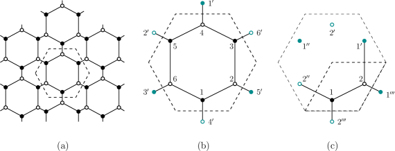
Figure 7. A discrete graph with symmetries $R$ and $F$.

Example 4.5.

It is easier to start with an example that has a richer structure, such as the periodic graph of Fig. 7(a). It is assumed that the black and white vertices have different potential, therefore $V$ symmetry is broken, while $R$ and $F$ symmetries are still present.

In part (b) the structure of the graph inside the dashed fundamental domain is magnified. Gray vertices outside of the fundamental domain are obtained by shifts from the corresponding vertices inside. For example, $f_{5^{\prime}}=\omega_{2}f_{5}$, therefore the operator $H(\vec{k})$ at site $2$ acts as

$$(H(\vec{k})f)_{2}=(f_{2}-f_{3})+(f_{2}-f_{1})+r(f_{2}-\omega_{2}f_{5})+q_{2}f_{2},$$

where we took the longer sides in the structure of Fig. 7(a) to have weight $1$ and the shorter sides weight $r$ (usually, the weight is taken to be inversely proportional to length). The entire operator $H(\vec{k})$ is

$$H(\vec{k})=\begin{pmatrix}q_{1}&-1&0&r\overline{\omega_{1}}\omega_{2}&0&-1\\ -1&q_{2}&-1&0&-r\omega_{2}&0\\ 0&-1&q_{1}&-1&0&-r\omega_{1}\\ r\omega_{1}\overline{\omega_{2}}&0&-1&q_{2}&-1&0\\ 0&-r\overline{\omega_{2}}&0&-1&q_{1}&-1\\ -1&0&r\overline{\omega_{1}}&0&-1&q_{2}\end{pmatrix},$$

with $\omega_{j}$ defined in (6); above, for simplicity, the potential $q$ was made to absorb the weighted degree of the corresponding vertex.

With $q_{1}=\sqrt{3}$, $q_{2}=0$ and $r=\sqrt{7}$, the eigenvalues of $H(\vec{k}^{*})$, calculated numerically, are

(51) $$-2.5097,\quad{-2.5097},\quad{-1.6753},\quad 3.4074,\quad 4.2418,\quad 4.2418.$$

To find the operator $Q_{1}$ acting on the two darker vertices in Fig. 7(c), we use the definition of the space $\mathcal{X}_{1}(\vec{k}^{*})$, equation (48): for the gray vertices we have

$$f_{1^{\prime}}=\tau f_{1},\quad f_{1^{\prime\prime}}=\overline{\tau}f_{1},\quad f_{2^{\prime}}=\tau f_{2}$$

by rotation and then

$$f_{1^{\prime\prime\prime}}=\overline{\tau}f_{1^{\prime\prime}}=\tau f_{1},\quad f_{2^{\prime\prime\prime}}=\tau f_{2^{\prime}}=\overline{\tau}f_{2}$$

by translation (see Fig. 2(c) with $\omega_{1}=\tau$ and $\omega_{2}=\overline{\tau}$). We thus get

$$Q_{1}=\begin{pmatrix}q_{1}&-1-\overline{\tau}-r\overline{\tau}\\ -1-\tau-r\tau&q_{2}\end{pmatrix}.$$

With the above choice of constants, the eigenvalues of $Q_{1}$ are

$$-2.5097\quad\mathrm{and}\quad 4.2418$$

which matches the double eigenvalues of $H(\vec{k}^{*})$ in (51). The matrices $Q_{0}$ and $Q_{2}$ can be similarly calculated as

$$Q_{0}=\begin{pmatrix}q_{1}&-2-\tau r\\ -2-\overline{\tau}r&q_{2}\end{pmatrix}\qquad\mbox{and}\qquad Q_{2}=\begin{pmatrix}q_{1}&-1-\tau-r\\ -1-\overline{\tau}-r&q_{2}\end{pmatrix}.$$

Example 4.6.

We will now explain the application of our theory to the most basic example: the tight-binding approximation of graphene structure, with vertices of a discrete graph representing carbon atoms, see Fig. 8(a).

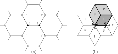
Figure 8. Graphene structure with two vertices per fundamental domain.

The operator $H(\vec{k})$ acts on a 2-dimensional space over vertices $1$ and $2$ (all other vertices of the graph are obtained by shifts). It acts as

$$(H(\vec{k})f)_{1} =-f_{2}-f_{2^{\prime}}-f_{2^{\prime\prime}}+qf_{1}$$

$$=-f_{2}-\omega_{1}f_{2}-\omega_{2}f_{2}+qf_{1},$$

and similarly for $(H(\vec{k})f)_{2}$. Note that the atoms are identical, hence $q_{1}=q_{2}=q$. When $\omega_{1}=\overline{\omega_{2}}=\tau$, the matrix $H$ is $q$ times identity.

The eigenproblem of the rhombic subdomain can be gleaned from Fig. 8(b). In particular, $f_{1}$ is forced to be zero: which can be seen from the equality $f_{1}=\tau f_{1}=\overline{\tau}f_{1}$ highlighted by the empty arrows in Fig. 8(b), or from the boundary conditions for the bottom right corner of Fig. 6(b). On the other hand, the value $f_{2}$ is unrestricted and $(Q_{1}f)_{2}=qf_{2}$. The complementary eigenfunction (eigenfunction of the operator $Q_{2}$) is localized on the vertex $1$.

5. Conical structure around a degeneracy

5.1. General perturbation theory

Here we list some general facts from the perturbation theory of operators depending on parameters, following [23, 45, 20]. Let

$$H(r)=H_{0}+(r-r_{0})H_{1}+O\left(|r-r_{0}|^{2}\right)$$

be an analytic family of self-adjoint operators depending on one parameter with an isolated doubly degenerate eigenvalue $\lambda_{0}$ at $r=r_{0}$. The eigenvalue then splits into two analytic branches

$$\lambda^{\pm}(r)=\lambda_{0}+\lambda_{1}^{\pm}(r-r_{0})+O\left(|r-r_{0}|^{2}\right).$$

The linear terms can be found as the eigenvalues of the $2\times 2$ matrix $PH_{1}P$, where $P$ is the projector onto the eigenspace of $\lambda_{0}$. The corresponding eigenvectors expand as

(52) $$\psi^{\pm}(r)=\psi^{\pm}_{0}+O\left(\frac{|r-r_{0}|}{|\lambda_{1}^{+}-\lambda_{1}^{-}|}\right),$$

where $\psi_{0}^{\pm}$ are the eigenvectors of $PH_{1}P$ (which are in the eigenspace of $H_{0}$). All eigenvectors are assumed to be normalized.

If $H=H(k_{1},k_{2})$ is an analytic function of two parameters and $\vec{k}_{0}$ is the point of double multiplicity of the eigenvalue $\lambda_{0}$, the one-parameter theory is still valid in every direction $\delta k_{1}=r\cos(\phi)$, $\delta k_{2}=r\sin(\phi)$. The parameters $\lambda_{1}^{\pm}$ now depend on the direction $\phi$.

We will say that a doubly degenerate eigenvalue is a conical point if $\lambda_{1}^{+}(\phi)\neq\lambda_{1}^{-}(\phi)$ in every direction; more precisely,

Definition 5.1.

Let $H(\vec{k})$ be an analytic family of self-adjoint operators. We will say that $H(\vec{k})$ has a nondegenerate conical point at $\vec{k}_{0}$ with an eigenvalue $\lambda_{0}$ if $\lambda_{0}\in\sigma_{d}(H(\vec{k}_{0}))$ is an isolated eigenvalue of geometric multiplicity $2$, and in an open neighborhood of $\vec{k}_{0}$ the eigenvalues are given by

(53) $$\lambda^{\pm}(\vec{k})=\lambda_{0}+\delta\vec{k}\cdot\vec{n}\pm\sqrt{Q(\delta\vec{k})}+O(|\delta\vec{k}|^{2}),\qquad\delta\vec{k}=\vec{k}-\vec{k}_{0},$$

where $\vec{n}\in\mathbb{R}^{2}$ and $Q(\vec{k})$ is a positive-definite quadratic form. The point $\vec{k}_{0}$ is a fully degenerate conical point if the same is true with $Q\equiv 0$.

From Lemma 3.1 we know that the points of double degeneracy at $\pm\vec{k}^{*}$ and $\vec{0}$ must either be nondegenerate circular cones (in $\varkappa$ coordinates) or fully degenerate cones. It turns out that the point $\vec{0}$ is always a fully degenerate cone; we will also derive a condition for nondegeneracy of the cone at $\pm\vec{k}^{*}$.

In the first order of perturbation theory (i.e. ignoring the $O(|\vec{\delta k}|^{2})$ term in (53)), the dispersion surface is given by the solution to

(54) $$\det\left(\delta k_{1}\,h_{1}+\delta k_{2}\,h_{2}-(\lambda-\lambda_{0})\right)=0,$$

where the $2\times 2$ Hermitian matrices $h_{1}$ and $h_{2}$ are given by

(55) $$h_{j}=\Phi^{*}\frac{\partial H}{\partial k_{j}}\Phi=\begin{bmatrix}\langle f_{1},\frac{\partial H}{\partial k_{j}}f_{1}\rangle&\langle f_{1},\frac{\partial H}{\partial k_{j}}f_{2}\rangle\\ \langle f_{2},\frac{\partial H}{\partial k_{j}}f_{1}\rangle&\langle f_{2},\frac{\partial H}{\partial k_{j}}f_{2}\rangle\end{bmatrix},\qquad j=1,\,2.$$

Here $\Phi=[f_{1},f_{2}]$ is a matrix whose columns are the orthonormal basis vectors of the degenerate eigenspace at $(0,0)$:

$$\Phi:\mathbb{C}^{2}\to\mathcal{X},\qquad\Phi:\begin{bmatrix}c_{1}\\ c_{2}\end{bmatrix}\mapsto c_{1}f_{1}+c_{2}f_{2}.$$

The projector $P$ onto the eigenspace is then given by $P=\Phi\Phi^{*}$.

5.2. Perturbation in the presence of symmetry

Naturally, the presence of symmetry imposes constraints on the form of the matrices $h_{1}$ and $h_{2}$. As we will see in Lemma XX and YY below, these constraints are often powerful enough to give an explicit form of the dispersion relation.

Lemma 5.2.

Let $H(\vec{k})$ be an analytic family of self-adjoint operators and the unitary operator $S$ satisfy

(56) $$SH(\vec{k})S^{*}=H(\hat{S}\vec{k}),$$

where the matrix $\hat{S}$ encodes the action of $S$ on the dual space. Let $\vec{k}_{0}$ be a fixed point of $\hat{S}$ and $[f_{1},\ldots,f_{m}]$ be an orthonormal basis of an eigenspace of $H(\vec{k}_{0})$. Let the unitary matrix $A_{S}$ encode the action of $S$ in this basis, namely

(57) $$S\Phi=\Phi A_{S},\qquad\mbox{where }\Phi:\mathbb{C}^{m}\to\mathcal{X},\ \Phi\vec{c}=c_{1}f_{1}+\ldots c_{m}f_{m}.$$

Then $h_{\vec{\delta k}}:=\delta k_{1}\,h_{1}+\delta k_{2}\,h_{2}$ satisfies

(58) $$A_{S}h_{\vec{\delta k}}A_{S}^{*}=h_{\hat{S}\vec{\delta k}}.$$

If $S$ is an antiunitary operator satisfying (56) and $S\Phi=\Phi A_{S}C$, then

(59) $$A_{S}h_{\vec{\delta k}}A_{S}^{*}=\overline{h_{\hat{S}\vec{\delta k}}}.$$

Proof.

From equation (56) we have

$$S\left(H(\vec{k}_{0}+\vec{\delta k})-H(\vec{k}_{0})\right)S^{*}=H\left(\hat{S}(\vec{k}_{0}+\vec{\delta k})\right)-H\left(\hat{S}\vec{k}_{0}\right)=H\left(\vec{k}_{0}+\hat{S}\vec{\delta k}\right)-H\left(\vec{k}_{0}\right),$$

where we used the fact that $\vec{k}_{0}$ is a fixed point of (19). Passing to the limit, we get

(60) $$S\left(\delta k_{1}\left.\frac{\partial H}{\partial k_{1}}\right|_{\vec{k}_{0}}+\delta k_{2}\left.\frac{\partial H}{\partial k_{2}}\right|_{\vec{k}_{0}}\right)S^{*}=:S\left(D_{\vec{\delta k}}H\right)S^{*}=D_{\hat{S}\vec{\delta k}}H,$$

where $D_{\vec{\delta k}}H$ is the directional derivative of $H$ in the direction $\vec{\delta k}$ at the point $\vec{k}_{0}$.

Note that $h_{\vec{\delta k}}=\Phi^{*}\left({D_{\vec{\delta k}}H}\right)\Phi$. Conjugating equation (60) by the matrix $\Phi$, we get (58) (note that $A_{S^{*}}=A_{S}^{*}$). The antiunitary case is analogous. ∎

5.3. Application to graphene operators

Lemma 5.3.

Let the self-adjoint operator $H$ be $\Gamma$-periodic and invariant under rotation $R$. If $H(\vec{k}^{*})$ has an eigenvalue $\lambda_{0}$ of multiplicity two with eigenvectors satisfying

(61) $$Rf_{1}=\tau f_{1},\qquad Rf_{2}=\overline{\tau}f_{2},\qquad\tau=e^{2\pi i/3},$$

the dispersion relation has the form $\lambda-\lambda_{0}=\pm|\alpha||\vec{\varkappa}-\vec{\varkappa}_{0}|+O(|\vec{\varkappa}-\vec{\varkappa}_{0}|^{2})$, with

(62) $$\alpha=\left\langle f_{1},\frac{\partial H}{\partial\varkappa_{1}}f_{2}\right\rangle.$$

Remark 5.4.

This calculation was performed for $\mathbb{R}^{2}$ Laplacian with any $R$-symmetric potential in [15, Prop 4.2], using explicit calculation of the derivatives ${\partial H}/{\partial\varkappa_{j}}$. We show that it is a direct corollary of Lemma 5.2.

Proof.

We use Lemma 5.2 with the symmetry $S=R$. From (61) we obtain

(63) $$A_{R}=\begin{pmatrix}\tau&0\\ 0&\overline{\tau}\end{pmatrix}.$$

Using the explicit form of the matrix $\hat{R}$ from (16), equation (58) can be written in components as

(64) $$\begin{pmatrix}\tau&0\\ 0&\overline{\tau}\end{pmatrix}h_{1}\begin{pmatrix}\overline{\tau}&0\\ 0&\tau\end{pmatrix}=-h_{1}-h_{2},\qquad\begin{pmatrix}\tau&0\\ 0&\overline{\tau}\end{pmatrix}h_{2}\begin{pmatrix}\overline{\tau}&0\\ 0&\tau\end{pmatrix}=h_{1}.$$

It is now straightforward to check that any $2\times 2$ Hermitian matrices satisfying (64) must be of the form

(65) $$h_{1}=\begin{pmatrix}0&\beta\\ \overline{\beta}&0\end{pmatrix},\qquad h_{2}=\begin{pmatrix}0&\tau\beta\\ \overline{\tau}\overline{\beta}&0\end{pmatrix},\qquad\mbox{where }\beta=\left\langle f_{1},\frac{\partial H}{\partial k_{1}}f_{2}\right\rangle.$$

We now calculate the shape of the dispersion relation in the first order of perturbation theory using (54). It is

(66) $$(\lambda-\lambda_{0})^{2}-|\beta|^{2}|\delta k_{1}+\tau\,\delta k_{2}|^{2}=(\lambda-\lambda_{0})^{2}-\frac{3}{4}|\beta|^{2}|\delta\varkappa|^{2}=0,$$

where we changed to the coordinates $\vec{\varkappa}=k_{1}\vec{b_{1}}+k_{2}\vec{b_{2}}$ in which the dispersion relation is the circular cone with no tilt. To relate the answer to (62), we observe that

$$\frac{\partial H}{\partial\varkappa_{1}}=\frac{\sqrt{3}}{2}\left(\frac{\partial H}{\partial k_{1}}+\frac{\partial H}{\partial k_{2}}\right),$$

and therefore, from (65), $\alpha=\frac{\sqrt{3}}{2}(1+\tau)\beta$. Since $|\alpha|^{2}=\frac{3}{4}|\beta|^{2}$, we get the promised answer. ∎

The cone becomes degenerate if $\alpha=0$ (this condition is equivalent to condition (4.1) of [15]). In [20], $\alpha$ was shown to be non-zero for small $\varepsilon$ in $H_{\varepsilon}=-\Delta+\varepsilon q(\vec{x})$; by analyticity, the cone can be degenerate only for isolated values of the parameter $\varepsilon$. We explore this in more detail in the next section.

5.4. Perturbation of the pure Laplacian

In this section we describe in more detail the case of Laplacian on $\mathbb{R}^{2}$ with the bounded potential $q(\vec{x})$ considered as a perturbation, $H_{\varepsilon}=-\Delta+\varepsilon q(\vec{x})$. Similar calculation appeared in [20] and [15] (see also [13]), therefore we concentrate on connections with the results presented above.

Proof of Theorem 2.5.

When $\varepsilon=0$, the lowest eigenvalue of $H_{0}(\vec{k}^{*})$ is triply degenerate. Indeed, the function

(67) $$\phi(\vec{x}):=\exp\left(i\vec{\varkappa}^{*}\cdot\vec{x}\right)=\exp\left(\frac{4\pi i}{3}x_{2}\right)$$

is an eigenfunction of the Laplacian and satisfies

$$\phi(\vec{x}+\vec{a}_{1})=\tau\phi(\vec{x}),\qquad\phi(\vec{x}+\vec{a}_{2})=\overline{\tau}\phi(\vec{x}),$$

therefore it is an eigenfunction of $H_{0}(\vec{k}^{*})$. Since $R$, the operator of rotation by $2\pi/3$, commutes with $H_{0}(\vec{k}^{*})$, the functions

(68) $$R\phi=\exp\left(\frac{4\pi i}{3}\left(-\frac{\sqrt{3}}{2}x_{1}-\frac{1}{2}x_{2}\right)\right),\qquad R^{2}\phi=\exp\left(\frac{4\pi i}{3}\left(\frac{\sqrt{3}}{2}x_{1}-\frac{1}{2}x_{2}\right)\right),$$

are also eigenfunctions. It can be verified directly that they are orthogonal. Their combinations

(69) $$\psi_{j}(\vec{x}):=\frac{1}{3}\left(\phi(\vec{x})+\tau^{j}R\phi(\vec{x})+\overline{\tau}^{j}R^{2}\phi(\vec{x})\right)=:P_{j}\phi,\quad j=0,1,2,$$

are simple eigenfunctions of the operator $H_{0}(\vec{k}^{*})$ restricted to $\mathcal{X}_{j}(\vec{k}^{*})$ for $j=0,1,2$ correspondingly.

We now need to show that the eigenvalues of $H$ in $\mathcal{X}_{0}(\vec{k}^{*})$ and $H$ in $\mathcal{X}_{1}(\vec{k}^{*})$ (or $\mathcal{X}_{2}(\vec{k}^{*})$) will separate for non-zero $\varepsilon$ as long as (14) is satisfied. In the first order perturbation theory, the condition for separation is

(70) $$\frac{\langle\psi_{0},q(\vec{x})\psi_{0}\rangle}{\langle\psi_{0},\psi_{0}\rangle}\neq\frac{\langle\psi_{1},q(\vec{x})\psi_{1}\rangle}{\langle\psi_{1},\psi_{1}\rangle}=\frac{\langle\psi_{2},q(\vec{x})\psi_{2}\rangle}{\langle\psi_{2},\psi_{2}\rangle}$$

where the scalar products are taken in $L^{2}(\Omega_{R})$. Since $\|\psi_{0}\|=\|\psi_{1}\|=\|\psi_{2}\|$ and $\tau+\overline{\tau}=-1$, condition (70) is equivalent to

(71) $$\left\langle P_{0}\phi,q(\vec{x})P_{0}\phi\right\rangle_{L^{2}(\Omega_{H})}+\tau\left\langle P_{1}\phi,q(\vec{x})P_{1}\phi\right\rangle_{L^{2}(\Omega_{H})}+\overline{\tau}\left\langle P_{2}\phi,q(\vec{x})P_{2}\phi\right\rangle_{L^{2}(\Omega_{H})}\neq 0.$$

Using that $P_{j}$ are projectors which commute with multiplication by the $R$-invariant function $q(x)$, we reduce the left-hand side to

(72) $$\left\langle(P_{0}+\overline{\tau}P_{1}+\tau P_{2})\phi,q(\vec{x})\phi\right\rangle=\langle R\phi,q\phi\rangle=\langle R^{2}\phi,qR\phi\rangle=\int_{\Omega_{H}}e^{\frac{4\pi i}{\sqrt{3}}x_{1}}q(\vec{x})\,d\vec{x},$$

in agreement with (14).

Two more facts are now needed to establish existence of non-degenerate conical points for almost all values of $\varepsilon>0$.

1. The parameter $\alpha$ describing the opening angle of the cone, see equations (62) and (66), is analytic as a function of $\varepsilon$.

2. $\alpha$ is nonzero when $\varepsilon=0$.

Analyticity of $\alpha=\alpha(\varepsilon)$ follows from the analyticity of the eigenfunction corresponding to a simple eigenvalue of the self-adjoint operator $H(\varepsilon)$ on the fixed space $\mathcal{X}_{1}(\vec{k}^{*})$ as a function of one parameter; this is a consequence of the results of Rellich and Kato, see [23, Sec. VII.3] and [35]. The corresponding eigenfunction $f_{1}$ is also analytic and so is $f_{2}$. The derivative $\partial H/\partial k_{1}=\partial H_{0}/\partial k_{1}$ does not depend on $\varepsilon$, therefore $\alpha$ defined by (62) is analytic.

Finally, we calculate the value of $\alpha(0)\neq 0$ explicitly. By the standard gauge transformation technique, $D_{\vec{\varkappa}}H=-2i\vec{\varkappa}\cdot\nabla$. Therefore, using (69) and orthogonality of $\phi$, $R\phi$ and $R^{2}\phi$, we get

$$\alpha =\frac{1}{\|\psi_{1}\|\|\psi_{2}\|}\left\langle\psi_{1},\frac{\partial H}{\partial\varkappa_{1}}\psi_{2}\right\rangle_{L^{2}(\Omega_{H})}=\frac{-2i}{\|\psi_{1}\|\|\psi_{2}\|}\left\langle\psi_{1},\frac{\partial}{\partial x_{1}}\psi_{2}\right\rangle$$

$$=\frac{-2i}{3\|\phi\|^{2}}\left\langle\phi+\tau R\phi+\tau^{2}R^{2}\phi,\frac{\partial}{\partial x_{1}}\left(\phi+\tau^{2}R\phi+\tau R^{2}\phi\right)\right\rangle$$

(73) $$=\frac{-2i}{3\|\phi\|^{2}}\left\langle\phi+\tau R\phi+\tau^{2}R^{2}\phi,-\frac{2\pi i}{\sqrt{3}}\tau^{2}R\phi+\frac{2\pi i}{\sqrt{3}}\tau R^{2}\phi\right\rangle=\frac{4\pi}{3\sqrt{3}}(-\tau+\tau^{2})=-\frac{4\pi i}{3}.$$

∎

Remark 5.5.

The assumption $q\in L^{\infty}(\mathbb{R}^{2})$ could be relaxed. The discreteness of spectrum and analyticity of eigenvalues of $H(\vec{k})$ (as functions of quasi-momenta $\vec{k}$) for periodic potentials $q\in L_{\mathrm{loc}}^{1+\varepsilon}(\mathbb{R}^{2})$, $\varepsilon>0$, follows from the argument in [3, Theorem 3.1] (where the corresponding result is obtained for the three-dimensional case when $q\in L_{\mathrm{loc}}^{3/2}(\mathbb{R}^{3})$). Under this assumption, the potential $q$ is a relatively bounded perturbation with relative bound zero and $H(\vec{k})$ is analytic family of type B in the sense of Kato [23].

Remark 5.6.

Consider a potential $q(\vec{x})$ which is $R$-invariant, but may not have $V$ or $F$ symmetry. It can be shown that the first order perturbation condition for the eigenvalues of $Q_{1}$ and $Q_{2}$ to not separate is precisely that the right hand side of equation (72) is real. The latter is of course satisfied if $q(\vec{x})$ does have $V$ or $F$ symmetry.

Example 5.7.

To continue with Example 4.5, it is interesting to investigate what happens when the parameter $r$ is equal to 1. At the special points $\pm\vec{k}^{*}$ there are now triple degeneracies as the spectrum of $Q_{0}$ coincides at this point with the spectra of $Q_{1}$ and $Q_{2}$. As a consequence there is no conical point there. Instead, the lower 3 sheets of the dispersion relation develop singularities along curves and touch each other to form an intricate picture, Figure 9. The picture can be resolved as three analytic surfaces crossing each other. Similar shape is assumed by the upper 3 sheets.

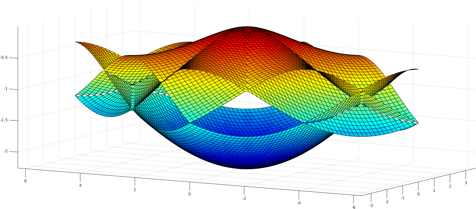
Figure 9. The lower three sheets of the dispersion relation for the graph in Example 4.5 with the parameter $r=1$.

The reason for such a complicated picture is that the system now has more symmetry and the three sheets can be obtained by (1) considering the smaller fundamental domain, (2) cutting up its dispersion relation and folding it back to Brillouin zone chosen in Figure 9. This is analogous to the situation with $H_{0}=-\Delta$ above which has more symmetry than the hexagonal lattice. It also illustrates the observation of [15] that the cones may degenerate at isolated values of a parameter ($r$, in the present example).

6. Degeneracy at $\vec{k}=\vec{0}$

The third fixed point of the rotation $\hat{R}$ in the momentum space (see Lemma 2.1) also leads to degeneracies in the spectrum. They are present even if both inversion and reflection symmetries are broken: rotation and complex conjugation are sufficient to retain degeneracies. However, the local structure of the dispersion relation is a degenerate cone, see Fig. 4 for an example.

Lemma 6.1.

Let the self-adjoint operator $H$ be $\Gamma$-periodic and invariant under rotation $R$. The space $\mathcal{X}(\vec{0})$ splits into the orthogonal sum

(74) $$\mathcal{X}(\vec{0})=\mathcal{X}_{0}(\vec{0})\oplus\mathcal{X}_{\perp}(\vec{0}),$$

where $\mathcal{X}_{0}(\vec{0})=\{\psi\in\mathcal{X}(\vec{0}):R\psi=\psi\}$. This splitting is $H$-invariant.

If $H$ is also invariant with respect to complex conjugation, then all eigenvalues of the operator $H$ restricted to $\mathcal{X}_{\perp}(\vec{k}^{*})$ have even multiplicity. Moreover, each eigenspace has an orthonormal basis $\{f^{1}_{n},f^{2}_{n}\}$, such that

(75) $$Rf^{1}_{n}=\tau f^{1}_{n},\qquad Rf^{2}_{n}=\overline{\tau}f^{2}_{n},\qquad\mbox{and}\qquad f^{2}_{n}=\overline{f^{1}_{n}}.$$

If $\lambda=\lambda_{0}$ is an eigenvalue of multiplicity two, then the dispersion relation is locally flat at $\vec{k}=\vec{0}$:

(76) $$\lambda-\lambda_{0}=O(|\vec{k}|^{2}).$$

Remark 6.2.

The eigenvalue $\lambda_{1}(\vec{0})$ is always non-degenerate, therefore first and second bands cannot touch at $\vec{k}=\vec{0}$.

Proof.

The proof of the first part is identical to the proof of Lemma 4.3 in the case of symmetries $R$ and $\overline{V}$.

To prove the estimate (76), we use the special basis satisfying (75). The proof of Lemma 5.3 still applies so the matrices $h_{1}$ and $h_{2}$ have the form given by (65). Applying Lemma 5.2 to the complex conjugation $C$ as an antiunitary symmetry of $H(\vec{k})$ at $\vec{k}=\vec{0}$, and using (75), we get

(77) $$\begin{pmatrix}0&1\\ 1&0\end{pmatrix}h_{\vec{k}}\begin{pmatrix}0&1\\ 1&0\end{pmatrix}=\overline{h_{-\vec{k}}}.$$

This is consistent with (65) only if $h_{\vec{k}}\equiv 0$. Then, according to (54), $\lambda-\lambda_{0}=O(|\vec{k}|^{2})$ yielding the conclusion. ∎

Remark 6.3.

More generally, one can get the following result. Suppose the operator $H(\vec{k})=H(k_{1},k_{2})$ has the following symmetry at the point $\vec{k}_{0}$:

$$H\left(\vec{k}_{0}-\vec{k}\right)=\overline{H\left(\vec{k}_{0}+\vec{k}\right)}:=CH\left(\vec{k}_{0}+\vec{k}\right)C^{-1}.$$

If $\lambda_{0}$ is an eigenvalue of $H(\vec{k}_{0})$ of multiplicity 2, it cannot be a nondegenerate conical point. In the leading order, it must have the form of two intersecting planes of which (76) is a degenerate example.

Figure 10. The operators $Q^{0}_{j}$ that together give the spectrum of $H(\vec{0})$.

Remark 6.4.

We can also obtain a more detailed splitting of $H(\vec{0})$ similar to Section 4.3, into a sum of three operators, $Q^{0}_{j}$, $j=0,1,2$, whose boundary conditions are described in Figure 10.

Example 6.5.

Revisiting Example 4.5 and calculating the eigenvalues of $H(\vec{0})$ numerically, we get

$$-3.8598,\quad{-0.9937},\quad{-0.9937},\quad 2.7257,\quad 2.7257,\quad 5.5918.$$

The corresponding operator $Q^{0}_{1}$ in this case can be shown to be

$$Q^{0}_{1}=\begin{pmatrix}q_{1}&-1-\overline{\tau}-r\tau\\ -1-\tau-r\overline{\tau}&q_{2}\end{pmatrix}.$$

with eigenvalues $-0.9937$ and $2.7257$.

Interestingly, in the case of Example 4.6, the graph structure is not rich enough to support the operators $Q^{0}_{1}$ or $Q^{0}_{2}$: it can be shown that in this case $\mathcal{X}_{\perp}(\vec{0})=\emptyset$.

In Appendix A we give a brief account of the case of pure Laplacian on $\mathbb{R}^{2}$ at the quasi-momentum point $\vec{k}=0$. It is largely parallel to Section 5.4, but requires delving deeper into representation theory of Section 4.1.

7. Persistence of conical points

We are now going to study the fate of the conical point when the rotational symmetry is broken by a small perturbation. We will consider two cases: when the perturbation retains the conjugate inversion symmetry $\overline{V}$ and when it retains the reflection symmetry $F$ (all other symmetries may or may not be broken). In both cases the conical point survives. Moreover, in the second case we are able to restrict the location of the surviving point to a line in $\vec{k}$ space. Of course, if the perturbation retains both symmetries, $\overline{V}$ and $F$, the stronger second result still applies.

7.1. Keeping $\overline{V}$ symmetry: Berry phase

Let us consider the weakly broken $R$ symmetry: we add to $H$ a perturbation which is $\overline{V}$-invariant but not $R$-invariant. The $F$ symmetry may or may not be preserved.

The tool for proving Theorem 2.6 in this case is the “Berry phase” [6, 36] (also known as “Pancharatnam–Berry phase” or “geometric phase”), of which we first give an informal description. Consider choosing a closed contour in the parameter space and tracking certain eigenvalue along this contour. The eigenvalue changes as we move along the contour, but we assume it remains simple. Now we choose the corresponding normalized eigenvector at every point of the contour. The eigenvector is defined up to a phase, and we choose it “in the most continuous fashion”. Once we completed the loop, the final eigenvector must equal the initial eigenvector up to a phase factor $e^{i\phi}$. The phase $\phi$ we call the Berry phase. The fact that it might be different from zero (modulo $2\pi$) in the simplest form of real operator $H$ and a contour encircling a conical point has been known for a while, see [22] and [2, Appendix 10.B].

We now argue that the Berry phase of the operator $H_{\varepsilon}(\vec{k})$ can only take values $0$ or $\pi$ (modulo $2\pi$). Because of the symmetry of the perturbation $W$, the perturbed operator $H_{\varepsilon}(\vec{k})$ will retain the symmetry $\overline{V}$ for all $\vec{k}$. The operator $\overline{V}$ is an antiunitary involution, i.e.

(78) $$\overline{V}(\alpha v)=\overline{\alpha}(\overline{V}v),\qquad\overline{V}^{2}=1,\qquad\langle\overline{V}v,\overline{V}u\rangle=\langle u,v\rangle.$$

If $\psi$ is a simple eigenfunction of $H(\vec{k})$, then, after multiplication by a suitable phase,

(79) $$\overline{V}\psi:=\overline{\psi(-\vec{x})}=\psi.$$

Indeed, because $\overline{V}$ commutes with the operator $H(\vec{k})$, $\overline{\psi(-\vec{x})}$ is an eigenvector with the same eigenvalue and thus equal to $e^{i\theta}\psi$ for some $\theta$. Multiplying $\psi$ by $e^{i\theta/2}$ makes it satisfy equation (79).

Condition (79) gives us a canonical way to choose the overall phase of the eigenvector, up to a sign. Now consider a closed path in the parameter $\vec{k}$ space. The phase acquired by a parallel section of the eigenspaces (the formal definition of the Berry phase) is restricted by condition (79): the factor must be either $+1$ or $-1$, so the phase is either $0$ or $\pi$ modulo $2\pi$.

On the other hand, the phase must change continuously upon a continuous deformation of the contour. Therefore, if the contour is homotopically equivalent to a point (i.e. encloses no parameter values where the eigenvalue becomes multiple), the phase must be equal to zero. But if the contour encloses a conical point, the phase is equal to $\pi$ modulo $2\pi$.

Lemma 7.1.

Let the self-adjoint operator $H(\vec{k})$, which analytically depends on the two parameters $\vec{k}=(k_{1},k_{2})$, have a nondegenerate conical point at $(0,0)$. Let $H(\vec{k})$ commute with an antiunitary involution $\overline{V}$. Then the Berry phase acquired on a contour enclosing the singularity $(0,0)$ is $\pi$.

Remark 7.2.

This result for a real-valued operator $H$ can be traced back at least to Herzberg and Longuet-Higgins [22]. Their proof is based on reducing the question using perturbation theory to a question about $2\times 2$ matrices and computing the eigenvectors explicitly. A more general formula is derived in [6, Sec. 3], from which Lemma 7.1 follows. In Appendix C we include an alternative derivation which avoids computing anything explicitly, opting instead for a more geometric explanation, which has interesting similarities to considerations of Section 7.2.

From this we immediately conclude that an isolated non-degenerate conical point cannot disappear under a perturbation which preserves the above symmetry.

Proof of Theorem 2.6 with $\overline{V}$ symmetry.

Surround the point with a small contour $\gamma$, such that inside this contour the eigenvalue $\lambda_{-}(\vec{k})$ of $H_{\varepsilon=0}(\vec{k})$, see (53), is simple except at $\vec{k}^{*}$. Then on contour $\gamma$ the Berry phase of the corresponding eigenfunction must be $\pi$.

For small values of $\varepsilon$, the eigenvalue on the contour $\gamma$ remains simple (as a continuous function on a compact set). Therefore, the phase must change continuously, so it must remain constant. Finally, if there were no multiplicity of $\lambda_{-,\varepsilon}(\vec{k})$ inside the contour, the Berry phase would be $0$. The multiplicity gives rise to a nondegenerate conical point by continuity. ∎

7.2. Keeping $F$ symmetry: parity exchange

Let us now consider the weakly broken $R$ symmetry: we add to $H$ a perturbation which is $F$-invariant but not $R$-invariant. The $V$ symmetry may or may not be preserved.

Proof of Theorem 2.6 with $F$ symmetry.

As explained in Section 3, $F$ remains a symmetry of the operator $H(\vec{k})$ when the quasi-momenta $\vec{k}$ satisfy $\omega_{2}=\overline{\omega_{1}}$ or, equivalently, $k_{2}=-k_{1}$ modulo $2\pi$.

Since the subgroup generated by $F$ has two representations, the space $\mathcal{X}(\vec{k})$ decomposes into two orthogonal subspaces, even and odd, defined by

(80) $$\mathcal{X}_{F}^{+}=\{\psi\in\mathcal{X}(\vec{k}):F\psi=\psi\} \mbox{``even''},$$

(81) $$\mathcal{X}_{F}^{-}=\{\psi\in\mathcal{X}(\vec{k}):F\psi=-\psi\} \mbox{``odd''}.$$

All simple eigenvectors of $H_{\varepsilon}(\vec{k})$ on the symmetry line belong to one or the other subspace. Multiple eigenspaces admit a basis consisting of vectors, each of which is either odd or even.

Now suppose we are at the special symmetry point $\vec{k}^{*}$ in the presence of rotational symmetry $R$ (i.e. $\varepsilon=0$). At the conical point we have a doubly degenerate eigenvalue with orthogonal eigenvectors which are mapped into each other by the transformation $F$ (see Lemma 4.3) and therefore the sum of these eigenvectors is even and the difference is odd with respect to $F$.

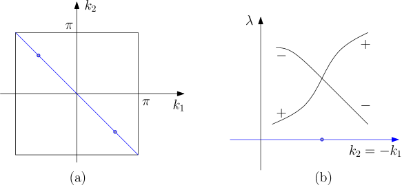
Figure 11. The line in the Brillouin zone where the symmetry $F$ is preserved (a). The form of the dispersion relation along the symmetry line (b).

Now consider the restrictions of the operator $H_{\varepsilon}$ with $\varepsilon=0$ onto the two subspaces $\mathcal{X}_{F}^{+}$ and $\mathcal{X}_{F}^{-}$. The above consideration shows that at the special point each restriction has a simple eigenvalue. As we go along the line $k_{2}=-k_{1}$, the eigenvalue of each restriction is an analytic function. These functions have an intersection at the point $k_{1}=-k_{2}=2\pi/3$. Since the two functions form a section of a non-degenerate cone, the intersection is transversal, see Fig. 11(b). Such intersection is stable under perturbation, and therefore, when we consider small $\varepsilon\neq 0$ (keeping the symmetry $F$), the intersection survives. Moreover, we know it remains on the line $k_{2}=-k_{1}$ and the only way it can disappear is by colliding with another degenerate eigenvalue on this line.

The intersection corresponds to a degenerate eigenvalue of the operator $H_{\varepsilon}(k)$ which, for small perturbations of the original potential, must still be a non-degenerate conical point. ∎

7.3. Destroying all symmetries

When a perturbation breaks all of the symmetries $R$, $V$ and $F$, the conical point normally separates into two surfaces, locally a two-sheet hyperboloid. This was discussed in detail in [15, Remark 9.2]. We merely remark here that the tips of the sheets of the hyperboloid give rise to the edges of the band spectrum. This provides an example for the band edges coming from a point in the bulk of the Brillouin zone, with no additional symmetries (since they have been broken), a subject first addressed on the mathematical level in [21, 12].

Appendix A Perturbation of pure Laplacian and degeneracy at $\vec{k}=0$

In this section we briefly outline the situation at the quasi-momentum point $\vec{k}=0$ when the operator is $H_{0}=-\Delta$. This should be compared with the discussion of Section 5.4.

The lowest eigenvalue of $H_{0}(0)$ is zero, its only eigenfunction is the constant function. The next eigenvalue is six-fold degenerate. The eigenfunctions are constructed out of the base function

(82) $$\phi(\vec{x}):=\exp\big{(}2\pi i(\vec{b}_{1}+\vec{b}_{2})\cdot\vec{x}\big{)}=\exp\left(\frac{4\pi i}{\sqrt{3}}x_{1}\right),$$

by rotations. The symmetries of this problem are the rotation $R$, inversion $V$, reflection $F$, and complex conjugation $C$. The group generated by $R$ and $V$ is the abelian group of rotations by $2\pi/6$, we denote this rotation by $R_{6}$. Then the six orthogonal eigenvectors are

(83) $$\psi_{j}(\vec{x}):=\sum_{k=0}^{6}\sigma^{jk}R_{6}^{k}\phi(\vec{x}),$$

where $\sigma=\exp(2\pi i/6)$ is the principal 6-th root of unity.

The six-fold degenerate eigenspace can be decomposed into four subspaces which correspond to the irreducible representations of the group of symmetries. Namely, $\xi=\psi_{0}(\vec{x})$ satisfies

$$R_{6}\xi=\xi,\qquad F\xi=\xi,\qquad C\xi=\xi,$$

eigenfunctions $\xi=\psi_{1}(\vec{x})$ and $\eta=-\psi_{5}(\vec{x})$ satisfy

$$R_{6}\begin{pmatrix}\xi\\ \eta\end{pmatrix}=\begin{pmatrix}\sigma\eta\\ \sigma^{5}\xi\end{pmatrix},\qquad F\begin{pmatrix}\xi\\ \eta\end{pmatrix}=\begin{pmatrix}\eta\\ \xi\end{pmatrix},\qquad C\begin{pmatrix}\xi\\ \eta\end{pmatrix}=\begin{pmatrix}\eta\\ \xi\end{pmatrix};$$

eigenfunctions $\xi=\psi_{2}(\vec{x})$ and $\eta=\psi_{4}(\vec{x})$ satisfy

$$R_{6}\begin{pmatrix}\xi\\ \eta\end{pmatrix}=\begin{pmatrix}\sigma^{2}\eta\\ \sigma^{4}\xi\end{pmatrix},\qquad F\begin{pmatrix}\xi\\ \eta\end{pmatrix}=\begin{pmatrix}\eta\\ \xi\end{pmatrix},\qquad C\begin{pmatrix}\xi\\ \eta\end{pmatrix}=\begin{pmatrix}\eta\\ \xi\end{pmatrix};$$

finally, $\xi=i\psi_{3}(\vec{x})$ satisfies

$$R_{6}\xi=-\xi,\qquad F\xi=-\xi,\qquad C\xi=\xi.$$

Perturbing the operator $H_{0}$ by a weak potential $\varepsilon q(\vec{x})$ which has all the symmetries $\{R,\,V,\,F,\,C\}$ will split this group of 6 eigenvalues into 4 groups corresponding to the above representations.

Appendix B Perturbation around a degenerate point with $F$ symmetry

It is interesting to calculate the matrices $h_{1},h_{2}$ if the degenerate eigenspace has $F$ symmetry. Suppose the basis is chosen such that

$$Ff_{1}=f_{1},\qquad Ff_{2}=-f_{2}.$$

This can be done at the special point $K$ if the operator has $R$ symmetry; in section 7.2 we showed that this situation survives even if we weakly break the symmetry $R$.

In this case, Lemma 5.2 yields

(84) $$\begin{pmatrix}1&0\\ 0&-1\end{pmatrix}h_{\vec{k}}\begin{pmatrix}1&0\\ 0&-1\end{pmatrix}=h_{\hat{F}\vec{k}},\qquad\hat{F}=\begin{pmatrix}0&-1\\ -1&0\end{pmatrix}.$$

It is easiest to evaluate $h_{\vec{k}}$ in the direction $\vec{k}_{e}=(1,-1)^{T}$, which is an eigenvector of $\hat{F}$ with eigenvalue 1, and in the direction $\vec{k}_{o}=(1,1)^{T}$, which is an eigenvector of $\hat{F}$ with eigenvalue $-1$. Remembering that $h_{-\vec{k}}=-h_{\vec{k}}$, we get

(85) $$h_{\vec{k}_{e}}=\begin{pmatrix}a&0\\ 0&c\end{pmatrix},\qquad h_{\vec{k}_{o}}=\begin{pmatrix}0&b\\ \overline{b}&0\end{pmatrix},$$

In particular, the trace of the derivative matrix in the direction perpendicular to the symmetry line $k_{2}=-k_{1}$ is zero and thus the cone can only be tilted in the direction of the symmetry line. If $R$ symmetry is present, there is no tilt, as mentioned above.

Appendix C Berry phase around a conical point

Here, for completeness, we give a proof of the fact that the Berry phase around a nondegenerate conical point is $\pi$, which has been formulated as Lemma 7.1. The proof is geometrical in nature and avoids the direct computation used in the original articles [22, 6].

Presence of the antiunitary symmetry $\overline{V}$ which squares to $-1$ allows us to choose special bases for eigenspaces. We will be using the following lemma.

Lemma C.1.

Let $A$ be an antiunitary involution on a separable Hilbert space $X$. Then

1. there is an orthonormal basis $\{f_{j}\}$ of vectors such that

   (86) $$Af_{j}=f_{j}.$$

2. if $\dim(X)=2$, there exists a basis $\{\psi,A\psi\}$.

Proof.

To prove the first part, we start with an arbitrary basis $\{\psi_{j}\}$. Then the vectors

$$f_{j}^{+}=\psi_{j}+A\psi_{j},\qquad\mbox{and}\qquad f_{j}^{-}=i(\psi_{j}-A\psi_{j})$$

both satisfy $Af=f$ and have the vector $\psi_{j}$ in their span. Therefore, the set $\{f_{j}^{+},f_{j}^{-}\}$ spans the whole space and can be made into a orthonormal basis by applying the Gram-Schmidt process. This preserves property (86) since all coefficients arising in the process are real:

$$\langle f,f^{\prime}\rangle=\langle Af,Af^{\prime}\rangle=\overline{\langle f,f^{\prime}\rangle}\in\mathbb{R}.$$

To get the second part from the first we start with the orthonormal basis $\{f_{1},f_{2}\}$ satisfying (86) and then take

$$\psi=(f_{1}+if_{2})/\sqrt{2},\qquad A\psi=(f_{1}-if_{2})/\sqrt{2},$$

which can be checked to be orthonormal. ∎

Now we are in the position to prove Lemma 7.1.

Proof of Lemma 7.1.

Representing the parameters around the location of the conical point in polar form we will study the limiting eigenvectors

(87) $$\psi_{0}^{\pm}(\theta)=\lim_{r\to 0}\psi^{\pm}(r,\theta),$$

where $\psi^{-}$ and $\psi^{+}$ are the eigenvectors of the lower and upper branches of the cone, correspondingly. We normalize these eigenvectors and fix the phase to have

(88) $$\overline{V}\psi^{\pm}=\psi^{\pm}.$$

Because the cone is nondegenerate (and thus $\left|\lambda_{1}^{+}(\theta)-\lambda_{1}^{-}(\theta)\right|>0$), the limit exists and is continuous in $\theta$, see equation (52).

Figure 12. Cone with a schematic representation of a circular contour (left); a cross-section of the cone by a plane through $\lambda$ axis in the direction $\phi$ (right).

The functions $\psi_{0}^{\pm}(\theta)$ have a curious property: since the section of the cone by a vertical plane is two intersecting lines, Fig. 12, the vector $\psi_{0}^{+}(\theta+\pi)$ is the same as $s_{1}\psi_{0}^{-}(\theta)$, where $s_{1}=\pm 1$.

We expand $\psi_{0}^{\pm}$ in a fixed basis of eigenvectors at the conical point, which we can choose to be of the form $\{\phi,\overline{V}\phi\}$,

$$\psi_{0}^{\pm}=\alpha^{\pm}(\theta)\phi+\beta^{\pm}(\theta)\overline{V}\phi.$$

From condition (88) we immediately get $\beta^{\pm}=\overline{\alpha^{\pm}}$. On the other hand, the vectors $\psi_{0}^{+}$ and $\psi_{0}^{-}$ are orthogonal, leading to the condition

$$\overline{\alpha^{+}}\alpha^{-}+\alpha^{+}\overline{\alpha^{-}}=0\qquad\mbox{or}\qquad\overline{\alpha^{+}}\alpha^{-}\in i\mathbb{R}.$$

From normalization of $\psi_{0}^{\pm}$, we conclude that $\alpha^{-}=i\alpha^{+}s_{2}$, where $s_{2}=\pm 1$. We therefore get

$$\alpha^{+}(\theta+\pi)=\alpha^{-}(\theta)s_{1}=i\alpha^{+}(\theta)s_{1}s_{2},$$

and, therefore,

$$\alpha^{+}(\theta+2\pi)=(is_{1}s_{2})^{2}\alpha^{+}(\theta)=-\alpha^{+}(\theta).$$

∎

We remark that in the proof above, the overall sign $s_{1}s_{2}$ determines the direction of rotation of the vectors $\psi_{0}^{\pm}(\theta)$ in the two-dimensional space.

References

- [1] V. I. Arnold. Modes and quasimodes. Funkcional. Anal. i Priložen., 6(2):12–20, 1972.
- [2] V. I. Arnold. Mathematical methods of classical mechanics, volume 60 of Graduate Texts in Mathematics. Springer-Verlag, New York, second edition, 1989. Translated from the 1974 Russian original by K. Vogtmann and A. Weinstein.
- [3] J. E. Avron and B. Simon. Analytic properties of band functions. Ann. Physics, 110(1):85–101, 1978.
- [4] O. Bahat-Treidel, O. Peleg, and M. Segev. Symmetry breaking in honeycomb photonic lattices. Opt. Lett., 33(19):2251–2253, 2008.
- [5] R. Band, O. Parzanchevski, and G. Ben-Shach. The isospectral fruits of representation theory: quantum graphs and drums. J. Phys. A, 42(17):175202, 42, 2009.
- [6] M. V. Berry. Quantal phase factors accompanying adiabatic changes. Proc. Roy. Soc. London Ser. A, 392(1802):45–57, 1984.
- [7] C. J. Bradley and B. L. Davies. Magnetic groups and their corepresentations. Rev. Modern Phys., 40:359–379, 1968.
- [8] P. Buser, J. Conway, P. Doyle, and K.-D. Semmler. Some planar isospectral domains. Internat. Math. Res. Notices, 1994(9):391–400, 1994.
- [9] A. Castro Neto, F. Guinea, N. Peres, K. Novoselov, and A. Geim. The electronic properties of graphene. Rev. Mod. Phys., 81:109–162, 2009.
- [10] Y. Colin de Verdière. Sur les singularités de van Hove génériques. Mém. Soc. Math. France (N.S.), 46:99–110, 1991. Analyse globale et physique mathématique (Lyon, 1989).
- [11] N. T. Do and P. Kuchment. Quantum graph spectra of a graphyne structure. Nanoscale Systems: Mathematical Modeling, Theory and Applications, 2:107–123, 2013.
- [12] P. Exner, P. Kuchment, and B. Winn. On the location of spectral edges in -periodic media. J. Phys. A, 43(47):474022, 8, 2010.
- [13] C. L. Fefferman, J. P. Lee-Thorp, and M. I. Weinstein. Topologically protected states in one-dimensional systems. preprint arXiv:1405.4569 [math-ph], 2014.
- [14] C. L. Fefferman, J. P. Lee-Thorp, and M. I. Weinstein. Honeycomb Schrödinger operators in the strong binding regime. preprint arXiv:1610.04930, 2016.
- [15] C. L. Fefferman and M. I. Weinstein. Honeycomb lattice potentials and Dirac points. J. Amer. Math. Soc., 25(4):1169–1220, 2012.
- [16] C. L. Fefferman and M. I. Weinstein. Wave packets in honeycomb structures and two-dimensional Dirac equations. Comm. Math. Phys., 326(1):251–286, 2014.
- [17] M. Golubitsky, I. Stewart, and D. G. Schaeffer. Singularities and groups in bifurcation theory. Vol. II, volume 69 of Applied Mathematical Sciences. Springer-Verlag, New York, 1988.
- [18] R. Goodman and N. R. Wallach. Symmetry, Representations, and Invariants, volume 255 of Graduate Texts in Mathematics. Springer New York, 2009.
- [19] C. Gordon, D. Webb, and S. Wolpert. Isospectral plane domains and surfaces via Riemannian orbifolds. Invent. Math., 110(1):1–22, 1992.
- [20] V. Grushin. Multiparameter perturbation theory of Fredholm operators applied to Bloch functions. Math. Notes, 86(5-6):767–774, 2009.
- [21] J. M. Harrison, P. Kuchment, A. Sobolev, and B. Winn. On occurrence of spectral edges for periodic operators inside the Brillouin zone. J. Phys. A, 40(27):7597–7618, 2007.
- [22] G. Herzberg and H. C. Longuet-Higgins. Intersection of potential energy surfaces in poluatomic molecules. Discuss. Faraday Soc., 35:77–82, 1963.
- [23] T. Kato. Perturbation theory for linear operators. Springer-Verlag, Berlin, second edition, 1976. Grundlehren der Mathematischen Wissenschaften, Band 132.
- [24] M. I. Katsnelson. Graphene: Carbon in Two Dimensions. Cambridge University Press, 2012.
- [25] P. Kuchment. Floquet theory for partial differential equations, volume 60 of Operator Theory: Advances and Applications. Birkhäuser Verlag, Basel, 1993.
- [26] P. Kuchment. An overview of periodic elliptic operators. Bull. Amer. Math. Soc. (N.S.), 53(3):343–414, 2016.
- [27] P. Kuchment and O. Post. On the spectra of carbon nano-structures. Comm. Math. Phys., 275(3):805–826, 2007.
- [28] A. Luican, G. Li, A. Reina, J. Kong, R. R. Nair, K. S. Novoselov, A. K. Geim, and E. Y. Andrei. Single-layer behavior and its breakdown in twisted graphene layers. Phys. Rev. Lett., 106:126802, Mar 2011.
- [29] J. L. Mañes. Existence of bulk chiral fermions and crystal symmetry. Phys. Rev. B, 85:155118, 2012.
- [30] J. L. Mañes, F. Guinea, and M. A. H. Vozmediano. Existence and topological stability of fermi points in multilayered graphene. Phys. Rev. B, 75:155424, 2007.
- [31] D. Monaco and G. Panati. Topological invariants of eigenvalue intersections and decrease of Wannier functions in graphene. J. Stat. Phys., 155(6):1027–1071, 2014.
- [32] K. Novoselov. Nobel lecture: Graphene: Materials in the flatland. Rev. Mod.Phys., 83:837–849, 2011.
- [33] O. Parzanchevski and R. Band. Linear representations and isospectrality with boundary conditions. J. Geom. Anal., 20(2):439–471, 2010.
- [34] L. A. Ponomarenko, R. V. Gorbachev, G. L. Yu, D. C. Elias, R. Jalil, A. A. Patel, A. Mishchenko, A. S. Mayorov, C. R. Woods, J. R. Wallbank, M. Mucha-Kruczynski, B. A. Piot, M. Potemski, I. V. Grigorieva, K. S. Novoselov, F. Guinea, V. I. Fal’ko, and A. K. Geim. Cloning of Dirac fermions in graphene superlattices. Nature, 497(7451):594–597, 2013.
- [35] F. Rellich. Störungstheorie der Spektralzerlegung, III. Math. Ann., 116(1):555–570, 1939.
- [36] B. Simon. Holonomy, the quantum adiabatic theorem, and Berry’s phase. Phys. Rev. Lett., 51(24):2167–2170, 1983.
- [37] J. C. Slonczewski and P. R. Weiss. Band structure of graphite. Phys. Rev., 109(2):272–279, 1958.
- [38] L. Tarruell, D. Greif, T. Uehlinger, G. Jotzu, and T. Esslinger. Creating, moving and merging Dirac points with a Fermi gas in a tunable honeycomb lattice. Nature, 483(7389):302–305, 2012.
- [39] J. von Neumann and E. Wigner. Ueber das verhalten von eigenwerten bei adiabatischen prozessen. Physik. Zeitschr., 30:467–470, 1929.
- [40] P. R. Wallace. The band theory of graphite. Phys. Rev., 71:622–634, May 1947.
- [41] J. R. Wallbank, A. A. Patel, M. Mucha-Kruczyński, A. K. Geim, and V. I. Fal’ko. Generic miniband structure of graphene on a hexagonal substrate. Phys. Rev. B, 87:245408, 2013.
- [42] H. Weyl. The Classical Groups. Their Invariants and Representations. Princeton University Press, Princeton, N.J., 1939.
- [43] E. P. Wigner. Group theory and its applications to the quantum mechanics of atomic spectra. Academic Press, New York, 1959.
- [44] M. Yankowitz, J. Xue, D. Cormode, J. D. Sanchez-Yamagishi, K. Watanabe, T. Taniguchi, P. Jarillo-Herrero, P. Jacquod, and B. J. LeRoy. Emergence of superlattice Dirac points in graphene on hexagonal boron nitride. Nat. Phys., 8:382–386, 2012.
- [45] M. G. Zaidenberg, S. Krein, P. A. Kuchment, and A. A. Pankov. Banach bundles and linear operators. Russian Math. Surveys, 30(5):115, 1975.
- [46] S. Zelditch. On the generic spectrum of a Riemannian cover. Ann. Inst. Fourier (Grenoble), 40(2):407–442, 1990.