Ion-specific colloidal aggregation:
population balance equations and potential of mean force

Abstract

Recently reported colloidal aggregation data obtained for different monovalent salts (NaCl, NaNO₃, and NaSCN) and at high electrolyte concentrations are matched with the stochastic solutions of the master equation to obtain bond average lifetimes and bond formation probabilities. This was done for a cationic and an anionic system of similar particle size and absolute charge. Following the series Cl^-, NO${}_{3}^{-}$, SCN^-, the parameters obtained from the fitting procedure to the kinetic data suggest: i) The existence of a potential of mean force (PMF) barrier and an increasing trend for it for both latices. ii) An increasing trend for the PMF at contact, for the cationic system, and a practically constant value for the anionic system. iii) A decreasing trend for the depth of the secondary minimum. This complex behavior is in general supported by Monte Carlo simulations, which are implemented to obtain the PMF of a pair of colloidal particles immersed in the corresponding electrolyte solution. All these findings contrast the Derjaguin, Landau, Verwey, and Overbeek theory predictions.

I Introduction

An extremely brief view of the well established colloidal aggregation picture under high electrolyte concentrations could be as follows Hunter : At sufficiently high electrolyte concentrations the repulsive electrostatic contribution to the Derjaguin, Landau, Verwey, and Overbeek (DLVO) potential turns negligible, and so, the colloid-colloid Hamaker attractive contribution dominates the effective interaction. Thus, all colloid-colloid (and cluster-cluster) collisions lead to the formation of irreversible and rigid bonds producing the so called diffusion limited cluster aggregation (DLCA) regime. The minimum electrolyte concentration needed to produce DLCA (in practice, to produce the maximum overall aggregation kinetics) is called critical coagulation concentration. Since this concentration corresponds to the total screening of the electrostatic contribution of the DLVO potential, larger amounts of electrolyte do not change the obtained DLCA kinetics.

In the above described view, valence and hydrated ionic size are considered (without taking into account the ion-ion short range correlations), while the nature of the employed electrolyte is completely disregarded. This contrasts a very large number of experimental observations which point out the specificity of some effective ion-surface interactions. Indeed, it has been clear for over a century the existence of systematic ion effects (widely known as Hofmeister effects Collins85 ; Cacace97 ; Boinovich10 ), which are strongly dependent on the ionic nature. These effects refer to the specificity manifested by certain ions on a plethora of phenomena, including surface tension at the air-water interface, heats of hydrations, stability and solubility of proteins, etc. A full and precise description of these effects must consider ion-surface, ion-ion, ion-water, water-surface, water-water, and direct surface-surface interactions Tavares04 ; Manciu05 ; Bostrom05 ; Quesada-Perez10 ; Kalcher10 ; Boinovich10 . All these contributions are not additive and so, mathematical treatments should not consider them independently.

In recent work, more evidence was found pointing out the specificity of ion effects Lopez-Leon10 . In this case it was shown that colloidal aggregation kinetics of hydrophobic colloidal particles at high monovalent electrolyte concentrations is extremely sensitive to the nature of the anion. That is, Cl^- was found to produce the expected DLCA-like regime, whereas SCN^- at the same concentration produced a steady-state cluster size distribution (CSD). In this paper these experimental data are matched with the stochastic solutions of the master equation to gain further insight into the process kinetics. The produced parameters, bond average lifetimes and primary bond formation probabilities, point out to the existence of a colloid-colloid potential of mean force (PMF) barrier for all employed monovalent electrolytes (NaCl, NaNO₃, and NaSCN) and systems (positive and negative colloids). Furthermore, also for positive and negative colloidal particles, they suggest a shallowing trend for the PMF well depth and an increasing trend for the PMF barrier following the series Cl^-, NO3^-, SCN^-. Thus, Monte Carlo simulations were implemented to see whether or not these trends can be captured. For this purpose, the potentials of mean force of a pair of colloidal particles immersed in the corresponding electrolyte solutions are calculated by including colloid-ion and ion-ion dispersion contributions. As shown in the results section, the general trends suggested by the population balance analysis agree with those obtained from simulations.

The paper is structured as follows: Section II summarizes the employed methodology to extract bond average lifetimes and primary bond formation probabilities from the experimental CSDs. This section also presents the obtained fitted values. Section III gives details on the employed MC method to obtain the PMF of two colloidal particles immersed in an electrolyte solution, in correspondence with the experimental conditions. Sec. IV presents the MC results and links them with the obtained bond average lifetimes and primary bond formation probabilities. Conclusions are drawn in Sec. V.

II Population Balance Fitting

II.1 Theoretical background

In order to gain physical information from the experimental time evolutions of the CSD, the stochastic master equation gillespie77 ; thorn94 ; thorn95 corresponding to a reversible aggregation model, including both aggregation and fragmentation kernels elminyawi91 ; pefferkorn98 ; Feng08 , is solved to match them. This master equation is the stochastic analogous to the deterministic population balance equations smol16 ; smol17 (a detailed description of the model and the algorithm employed to stochastically produce the CSDs is given in reference Odriozola03 section 4.3). The model behind the mathematical treatment assumes that two kinds of bonds, primary and secondary, can be formed. Primary bonds occur in an energy minimum that is very close to the particle surface, and then, is associated to interactions between bare particles. Secondary bonds occur at a certain distance from the particle surface, and thus, refer to situations where an energetic barrier prevents particles from completely approaching. These two kinds of bonds have different breakup probabilities and are treated separately. The energetic barrier enters as the probability, $P_{1}$, to form a primary bond given that a bond is formed (thus, the probability for producing a secondary bond given that a bond is formed is $1-P_{1}$). Furthermore, since the model assumes no barrier to form the secondary bonds, all collisions are effective, i. e., collisions always lead to either primary or secondary bond formation. Therefore, the Brownian kernel can be used to model the aggregation kinetics of the system. This kernel is given by

$$k^{Brow}_{ij}=\frac{1}{4}k_{11}(i^{1/d_{f}}+j^{1/d_{f}})(i^{-1/d_{f}}+j^{-1/d_{f}})$$ (1)

where $k_{11}$ is the dimmer formation rate constant, and $d_{f}$ is the clusters’ fractal dimension. The fragmentation kernel $f_{ij}$ is given by

$$f_{ij}=e_{ij}(1\!+\delta_{ij})(1\!-\!P_{c})\left(\frac{E_{1}}{\tau_{1}(E_{1}\!+\!E_{2})}\!+\!\frac{E_{2}}{\tau_{2}(E_{1}\!+\!E_{2})}\right)$$ (2)

where $E_{1}$ and $E_{2}$ are the number of primary and secondary bonds in the system, $\tau_{1}$ is the average lifetime of primary bonds, $\tau_{2}$ is the average lifetime of secondary bonds, and $\delta_{ij}$ is the Kronecker delta function. $e_{ij}$ is the average number of bonds that, after breaking-up, leads to $i-$ and $j-$size fragments. This function was approached by averaging over all fragmentation possibilities of a vast collection of simulated cluster structures and is given in reference ruptura01 . Finally, $P_{c}=1-0.164(ij)^{-0.35}$ is the probability for two just produced clusters to collide and re-aggregate europhysics01 ; Lattuada03 ; Lattuada04 ; Lattuada06 . Both kernels are used to obtain the time evolution of the CSD by stochastically solving the population balance equations as explained in reference ruptura03 . As mentioned, $P_{1}$ is introduced in order to discern whether a primary or secondary bond is formed when a cluster-cluster collision occurs. The values of the parameters $k_{11}$, $P_{1}$, $\tau_{1}$, and $\tau_{2}$ result from fitting the solutions of the population balance equations to the experimental CSDs. However, $k_{11}$ must have a fixed value independently of the employed anion (since the model states that every collision leads to bond formation and the viscosity variations are negligible). The best overall fits are obtained for $k_{11}=9.0\times 10^{-18}$ m${}^{3}/$s, which is a value within the boundaries of the $k_{11}$ range generally accepted for diffusion limited cluster aggregation sonntag87 , $k_{11}=(6.0\pm 3.0)\times 10^{-18}$ m${}^{3}/$s. The parameter $d_{f}$ was fixed to the typical value of DLCA, $d_{f}=1.8$ meakin98 , for the Cl^- ion, and to $d_{f}=2.0$ in the other cases. $P_{1}$, $\tau_{1}$, and $\tau_{2}$ were considered as free parameters. It should be noted that, by handling these parameters, the two classical aggregation regimes can be reproduced: i) DLCA lin90pcm when $P_{1}=1$ and $\tau_{1}\rightarrow\infty$, for all $\tau_{2}$ values; or $\tau_{1}\rightarrow\infty$, and $\tau_{2}\rightarrow\infty$ for all $P_{1}$; or $P_{1}=0$ and $\tau_{2}\rightarrow\infty$, for all $\tau_{1}$ and ii) Reaction limited cluster aggregation (RLCA) lin90pra when $\tau_{2}=0$ and $\tau_{1}\rightarrow\infty$, being $P_{1}$ the sticking probability. Therefore, this reversible model contains DLCA and RLCA as limiting cases. These limiting cases were tested to make sure the correctness of the implemented algorithm.

II.2 Fitted curves and parameters ($P_{1}$, $\tau_{1}$, and $\tau_{2}$)

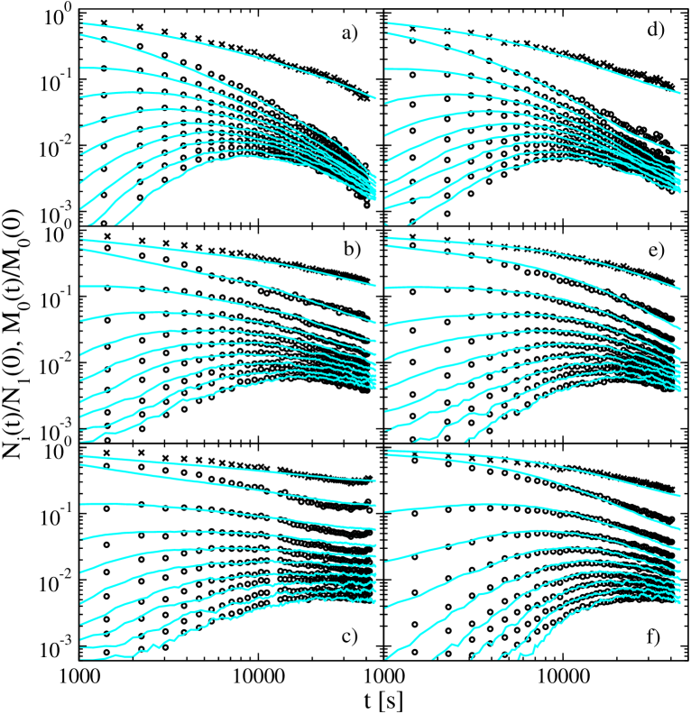
Figure 1: Time evolutions of the normalized CSDs, $N_{i}(t)/N_{1}(t\!=\!0)$, for the aggregation induced by a) NaCl, b) NaNO₃, and c) NaSCN and positive colloidal particles. Panels d), e), and f) correspond to the aggregation of negative colloidal particles under the same electrolytes, respectively. Open circles are the experimental CSDs (from monomers up to clusters having nine particles) whereas crosses correspond to the normalized total number of clusters, $M_{0}(t)/M_{0}(t\!=\!0)$ (data taken from Lopez-Leon10 ). Lines are the theoretical fits.

Table 1: $P_{1}$, $\tau_{1}$, and $\tau_{2}$ values of both latices when aggregation is induced by different electrolytes. Fitting errors are less than 20$\%$ in all cases. Mobility data, $\mu_{e}$, are also included (taken from Lopez-Leon10 ).

	Cationic				Anionic
	$\mu_{e}$ $10^{8}$ [m${}^{2}/$Vs]	$\tau_{1}$ [s]	$\tau_{2}$ [s]	$P_{1}$	$\mu_{e}$ $10^{8}$ [m${}^{2}/$Vs]	$\tau_{1}$ [s]	$\tau_{2}$ [s]	$P_{1}$
NaCl	$0.79\pm 0.18$	$>1\times 10^{6}$	2000	0.33	$-1.17\pm 0.10$	200000	400	0.30
NaNO3	$-0.03\pm 0.19$	100000	600	0.07	$-1.27\pm 0.10$	200000	150	0.06
NaSCN	$-0.90\pm 0.09$	25000	370	0.04	$-1.37\pm 0.10$	200000	100	0.04

As mentioned, the probability of forming a primary bond given a particle-particle collision, $P_{1}$, and the average lifetime of primary and secondary bonds, $\tau_{1}$, and $\tau_{2}$, are taken as free parameters to fit the experimental CSDs. The resulting curves ($N_{i}(t)/N_{1}(t\!=\!0)$, being $N_{i}(t)$ the number of $i$-size clusters at time $t$) are plotted in panels a)-c) of Fig. 1 for the positively charged particles and in panels d)-f) of the same figure for the negatively charged ones, where the points refer to the experimental data and the lines to the stochastic solutions of the master equation. In this figure, panels a) and d), b) and e), and c) and f) show the data obtained under NaCl, NaNO₃, and NaSCN, respectively. Additionally, all panels show the normalized total number of clusters, $M_{0}(t)/M_{0}(t\!=\!0)$ ($M_{0}(t)=\sum_{i=1}^{i=\inf}N_{i}(t)$), as crosses (experimental) and cyan lines (fits). The obtained values of the fitted parameters are listed in Table 1. The obtained agreement between experimental results and theoretical fits is good for all cases.

It is common saying that three parameters are enough to fit practically any well behaved curve. So, the question -how much can we trust the values of the fitted parameters?- naturally arises. To answer it one should take into account that not only a single curve, but a very important part of the whole CSD is being fitted with the employed parameters (oligomers evolution plus the total number of clusters). This adds much difficulty to the fitting procedure. Furthermore, the parameters have physical meaning and consequently cannot take any value. That is, $P_{1}$ is restricted to $0\leq P_{1}\leq 1$, and $0\leq\tau_{2}\leq\tau_{1}$. Once that is said, it should be pointed out some limitations of the employed model. The construction of function $e_{ij}$ is based on loop-less aggregates hiving a fixed fractal dimension, $d_{f}\approxeq 2.0$. On the one hand, loop-less aggregates imply that all bond breaking events lead to cluster fragmentation. On the other hand, $e_{ij}$ is expected to increase with $d_{f}$. Both assumptions (loop-less aggregates and $d_{f}=2.0$) may not correspond to reality when bonds allow for the relative movement among the particles of a cluster (restructuring) Tirado-Miranda99 ; Babu08 . In this case, the clusters fractal dimension raises probably reaching values over 2.0. This in turn enters in equation 1, for which its solutions are luckily not very sensitive to this parameter Babu08 (a larger $d_{f}$ produce smaller cross sections which practically compensates the larger diffusion coefficients, although the small-large aggregation turns relatively less favorable). Notwithstanding, the fitted parameter values surely shift when restructuring occurs. Finally, it should also be mentioned that the employed method of hydrodynamic focusing of clusters, needed for obtaining the detailed experimental data, probably enhances breakup. For all these reasons, it is safer to consider trends to be reliable only.

When Cl^- acts as the counter-ion, i. e., for positive particles, a DLCA model with $k_{11}=6.0\times 10^{-18}$ m³/s ($P_{1}=1$ and $\tau_{1}>1\times 10^{6}$ s) provides a relatively good agreement with the experimental data (not shown). Nevertheless, the best fit is obtained for $k_{11}=9.0\times 10^{-18}$ m³/s, $P_{1}$ = 0.33, $\tau_{1}>1\times 10^{6}$, and $\tau_{2}=2000$ s, suggesting that, even for the fastest aggregation kinetics, there is always a small potential barrier that avoids reaching total effectiveness in the collisions between particles. Something similar occurs for the negative system when Na⁺ acts as the counterion (see Table 1). Although introducing extra fitting parameters is not an absolute requisite to fit the CSD induced by NaCl for both systems, it becomes imperative when NO${}_{3}^{-}$ or SCN^- act as the counter-ions. The CSDs induced by these anions cannot be explained without considering the formation of reversible bonds.

For positive particles and when NO${}_{3}^{-}$ is the counter-ion (Fig. 1 b)), the values of $P_{1}$, $\tau_{1}$, and $\tau_{2}$ importantly drop off: $P_{1}=0.07$, $\tau_{1}=100000$ s, and $\tau_{2}=600$ s. The pronounced decrease of $P_{1}$ signals an increase in the number of secondary bonds, whose lifetimes become also shorter. This would translate into a higher mean force potential barrier and a shallower secondary minimum. This trend is confirmed by the analysis of the anion having the larger dispersion contribution, SCN^-. In this case the rate between secondary and primary bonds induced by SCN^- increases with respect to NO${}_{3}^{-}$, and the lifetime of the bonds decreases, revealing the existence of weaker bonds between particles: $P_{1}=0.04$, $\tau_{1}=25000$ s, and $\tau_{2}=370$ s. Actually, in the regime induced by SCN^-, a balance between the number of new formed bonds and broken bonds is established Babu06 ; Babu07 ; Kovalchuk09a ; Kovalchuk09b . This produces a quasi-steady-state for $t\gtrsim 25000$s, where the average cluster size equals 2.45 particles/cluster. It should be noted that the evolution of the small species slightly increases at long times. This effect is produced by gravity Odriozola04 and is followed by an increase of the average cluster size (not captured) and a final depletion of the colloidal particles which accumulate at the flask bottom Wu03 ; Agustin06a ; Agustin06b .

When the particles are negatively charged, electrostatic forces are expected to hamper the specific accumulation of anions, which now act as co-ions, at the particle surface. For this reason, the average lifetime of primary bonds is expected to be less influenced by the anions nature. This is in agreement with the large and constant $\tau_{1}$ values shown in Table 1 for all electrolytes. Since we use sodium salts for all cases, the cation in solution is always the same independently of the salt employed, while the anions change. It hence follows that only counter-ions have an effect on $\tau_{1}$. From this result, it seems that anions are easily removed from the bonding area when the particles are negatively charged (note that this area is the co-ions less favorable electrostatic region to be placed). Conversely, $P_{1}$ and $\tau_{2}$ highly depends on the co-ion in solution, indicating that co-ions play an important role at slightly larger interparticle distances. The value of $\tau_{2}$ gradually decreases by increasing the dispersion contribution of the anions, suggesting that the secondary potential minimum is progressively shifted away from the particle surface, where the Hamaker force is smaller. This result emphasizes the important role of non-DLVO contributions on the PMF, even when the anions (the ions expected to specifically adsorb at the colloid surfaces) act as co-ions. Interestingly, $\tau_{2}$ attains smaller values in the anionic latex than in the cationic one. This could be due to the fact that a higher number of sodium ions are necessary to screen the more important effective charge of the anionic particles (the effective charge is expected to increase due to the specific anion adsorption). As a result, all secondary minima would shift away from the particle surface. Finally, $P_{1}$ is practically independent of the sign of the particles although strongly depend on the anion nature.

In brief, following the series Cl^-, NO${}_{3}^{-}$, SCN^-, the parameters obtained from the fitting procedure to the CSD suggest: i) An increasing trend for the PMF barrier for both, the cationic and the anionic system, according to the $P_{1}$ decreasing trend. ii) An increasing trend for the potential of mean force at contact, for the cationic system, and a practically invariant value for the anionic system. This is in correspondence with the obtained decrease of $\tau_{1}$ for the cationic system and the constant value of $\tau_{1}$ for the anionic colloidal particles. iii) A decreasing trend for the depth of the secondary minimum, in agreement with the decreasing values of $\tau_{2}$ for both latices. Additionally, the depth of the secondary minima for all electrolytes and for the anionic case should be smaller than those corresponding to the cationic case. iv) Finally, an increasing trend for the adsorption of anions for both systems. This is to agree with the increase of the mobility values obtained for the anionic system, as well as with the mobility reversal of the cationic particles (see the mobility data included in Table 1). The PMF from Monte Carlo simulations should capture these trends.

III Simulation details

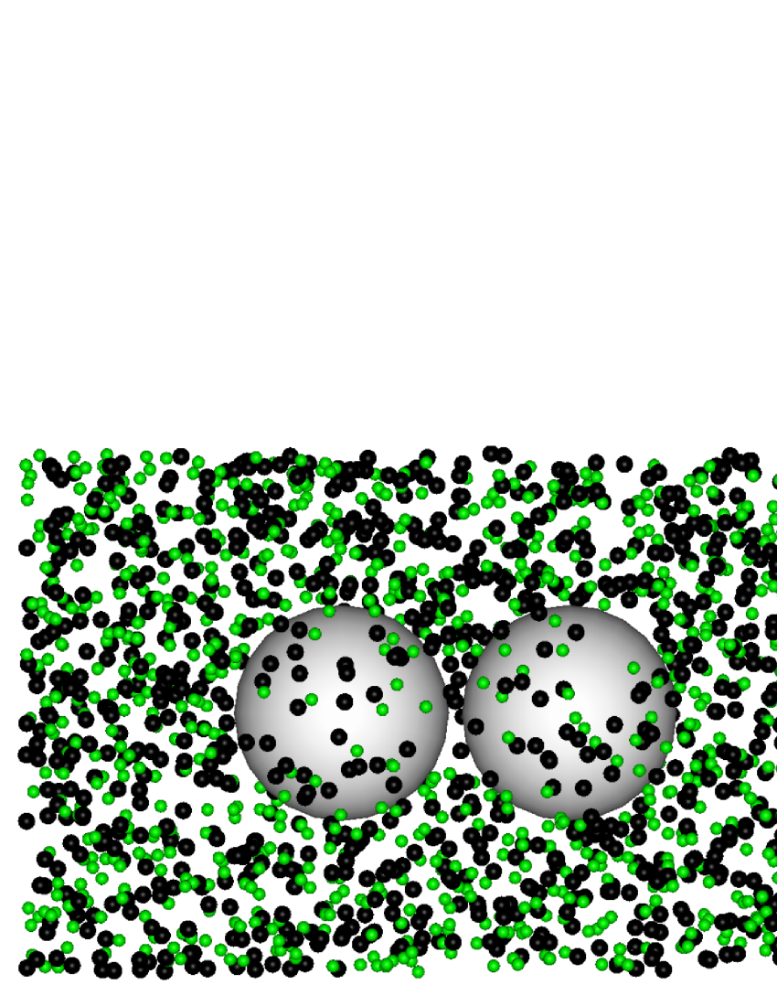
Figure 2: Snapshot of an equilibrated configuration of the system. Colloidal particles are white, light green particles are coions, and black particles are counterions.

Canonical Monte Carlo (MC) simulations are implemented for obtaining the PMF between two like-charged colloidal particles immersed in a 1-1 electrolyte. The macroparticles (colloidal particles) radius is $a_{M}=25\mbox{\AA}$ and carry the charge which corresponds to $\sigma=\pm 50$ mC/m² at their center. Two colloidal particles are fixed in the simulation box at a surface-surface distance $h$ from one another. These particles remain fixed during a simulation run (only ions are allowed to explore the configuration space). Several surface-surface distances, $h$, are independently set as different runs to build the PMF. The simulation box is a prism having $L_{x}=L_{y}=120\mbox{\AA}$, and $L_{z}=250\mbox{\AA}$, sides much larger than the Debye-Hückel screening length for all studied cases. This condition is important to avoid size effects. The origin of coordinates is set at the prism center and periodic boundary conditions are set for the three directions. The 1-1 electrolyte is modeled by hard spheres of radius $a_{c}$ (cation) and $a_{a}$ (anion) with a centered point charge. As for the real experiment, an electrolyte concentration of $0.6$M is set. Additional ions are added to make the system electroneutral. Initially, these electrolyte particles are randomly placed avoiding overlaps. Similar system setups were employed elsewhere to study forces between fixed colloidal particles Felipe05 ; Odriozola06 . The rout for obtaining the PMF is that described in references Felipe05 ; Odriozola06 ; Tavares04 ; Bostrom06 . This type of simulations is frequently employed to compare the resulting PMF with those obtained by integral equations and density functional theories Felipe05 ; Lima07 ; Jin11 .

All excluded volume interactions are modeled by hard interactions. That is, overlaps are always rejected and non overlapping configurations are given a null excluded volume contribution to the configuration energy. On the other hand, the electrostatic contribution between any pair of sites $ij$, where $i$ and $j$ are either charged sites of the colloidal particles or ions, is given by

$$U_{el}=k_{B}Tl_{B}\frac{z_{i}z_{j}}{r_{ij}}$$ (3)

where $r_{ij}$ is the distance between sites $i$ and $j$, and $z_{i}$ and $z_{j}$ are the valences of sites $i$ and $j$, respectively. The electrostatic strength is given by the Bjerrum length, i. e., by

$$l_{B}=\frac{e^{2}}{\varepsilon k_{B}T}$$ (4)

where $\varepsilon$ is the dielectric constant. $l_{B}=7.14\mbox{\AA}$ is set for water at $T=298$K. Finally, dispersion contributions are added to the configuration energy for the ion-macroparticle and for the ion-ion interaction. They read

$$\begin{array}[]{ll}U^{im}_{disp}=-\frac{B_{im}}{r^{3}_{im}}\\ U^{ij}_{disp}=-\frac{B_{ij}}{r^{6}_{ij}}\end{array}$$ (5)

being $B_{im}$ the dispersion parameter for the $i$-ion and the macroparticle (cation-macroparticle, anion-macroparticle) and $B_{ij}$ the dispersion parameter for the $ij$ ion-ion contribution (cation-cation, anion-anion, anion-cation). The values for these parameters are taken from Tavares et al. and Boström et al. Tavares04 ; Bostrom06 . Electrostatic interactions are treated using the Ewald summation formalism. The convergence factor was fixed to 5.6/$L_{x}$. There were set five reciprocal lattice vectors for $x$ and $y$ directions and six for the $z$ direction. A snapshot of an equilibrated configuration for positive colloidal particles and NaCl, (with $a_{c}=1.5\mbox{\AA}$, $a_{a}=2\mbox{\AA}$) is shown in Fig. 2.

The effective electrostatic force acting on colloidal particle $m$ is obtained by simply accounting for all sites contributions, i. e., by computing

$$F_{el}=<\sum_{i}-\nabla U_{el}(r_{im})>$$ (6)

where $i$ runs over all sites except the corresponding colloidal particle site. The same procedure applies to the dispersion contribution, leading to

$$F_{disp}=<\sum_{i}-\nabla U^{im}_{disp}(r_{im})>.$$ (7)

On the other hand, the contact force contribution (also called collision contribution Tavares04 ; Bostrom06 ) is obtained by integrating the ions contact density at the colloidal particle surface, $\rho_{c}$, i. e., by means of

$$F_{c}=-\int_{S}\rho_{c}k_{B}T\hat{\mathbf{n}}ds$$ (8)

In this case we approach $\rho_{c}$ at $ds$ by extrapolating the density of each species close to the surfaces. Finally, it should be mentioned that all these contributions to the net force are interdependent.

IV Results

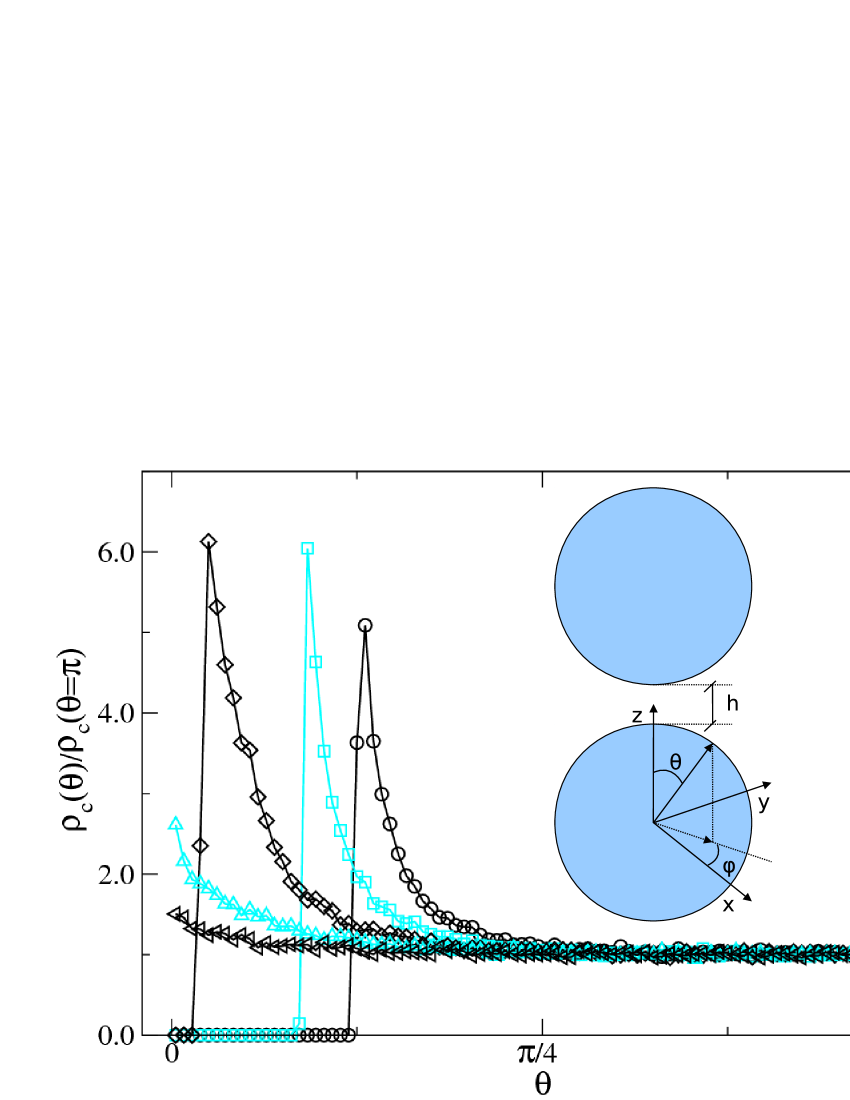
Figure 3: Normalized counterion surface density, $\rho_{c}(\theta)/\rho_{c}(\theta\!=\!\pi)$, as a function of the polar angle $\theta$ for the positive system under NaCl. Dark circles, light squares, dark diamonds, light triangles, and dark triangles correspond to $h=$0, 2, 4, 6, and 10Å, respectively. The inset shows the employed spherical coordinate system.

Simulations are performed to gain insight into the mechanisms through which different monovalent anions lead to different overall aggregation kinetics. Nonetheless, even without taking into account many details such as water structure, surface charge distribution, and roughness, among others, we can only study much smaller particles than the ones employed in the real experiments (100 times smaller). Thus, only trends are expected to be comparable with the data obtained from experiments.

As mentioned in section III, the PMF acting on both colloidal particles at a fixed distance can be accessed by ensemble averaging all its contributions. To understand their behavior it is convenient to first take a look at the ionic density profile on the surface of the colloidal particles. This profile is shown for the counterions (Cl^-) and for the cationic system in Fig. 3. Different symbols correspond to different surface-surface separation distances, $h$. The inset of the same figure shows the definitions of angles $\theta$ and $\varphi$ (in spherical coordinates). By symmetry, surface ionic densities do not depend on $\varphi$. For $h=0$, there is an excluded region for $\theta\lesssim\pi/8$. That is, anions cannot enter in-between the colloidal particles. For slightly larger $\theta$, a large peak is produced, pointing out a strong counterion accumulation occurring at the surfaces of both colloidal particles (these peaks are absent for coions, Na⁺, as expected). The reason for this to occur is twofold. On the one hand, in that region counterions are attracted by the electrostatic and dispersion forces of both particles (counterions are placed in contact to both macroparticles surfaces). In fact, this peak is placed where counterions minimize their electrostatic energy. On the other, the large surface/volume relationship of the region favors entropic adsorption (by increasing the accessible volume of other ions). For larger $\theta$ the counterion surface density monotonically decreases reaching a constant value for $\theta\gtrsim\pi/4$. The inhomogeneous distribution of ions around the dumbbell is responsible for the appearance of indirect forces between the macroparticles (see equations 6-8). There is no net force acting on $x$ and $y$, as the ionic distribution is symmetric around the $z$ axis (independent of $\varphi$). The inhomogeneity in $\theta$ produces forces in the $z$ direction only. Hence, the large accumulation of counterions at both macroparticles surfaces should produce a large repulsive contact contribution to the overall interaction force, since these ions are pushing the colloidal surfaces away in order to enter the low-energy interparticle region, but, in turn, they should also attract the colloidal particles by electrostatic and dispersion forces (bridging). Conversely, the counterions adsorbed at large $\theta$ are producing contributions to the force in the opposite direction, and so, they may counterbalance the peak effect since they act on a larger surface area (there is no excluded region at large $\theta$). The net force is the sum of these intricate contributions to the direct colloid-colloid interaction.

As the macroparticles separation distance $h$ increases, the surface density peak grows and shifts to smaller values of $\theta$. These two facts would yield larger contributions of the forces in the $z$ direction. For $h=2a_{a}$ (the counterion diameter), the height of the peak reaches a maximum, decreasing for larger values of $h$. The peak is now placed in the inter-particle region, i. e., at the point of zero electric field (center of the simulation box) where counterions minimize their electrostatic energy. Thus, for $h=2a_{a}$, the counterions can access all macroparticles surfaces and the in-between excluded region disappears. For $h>2a_{a}$ the peak’s height rapidly decreases as $h$ increases. However, it completely vanishes at large $h$ where the double layers become totally independent of each other and the net colloidal forces fade out.

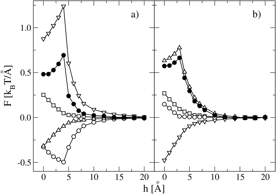
Figure 4: Forces acting on the colloidal particles as a function of their surface-surface separation distance, $h$. a) For positive colloidal particles. b) For negative colloidal particles. Squares, circles, triangles up, and triangles down correspond to the electrostatic, dispersive, Na⁺-contact, and Cl^--contact, force contributions. Bullets correspond to the net force.

For NaCl with $a_{c}=1.5\mbox{\AA}$ and $a_{a}=2.0\mbox{\AA}$, the force contributions are shown in Fig. 4 a) for cationic colloidal particles, and in Fig. 4 b) for anionic colloidal particles. Let’s focus first in Fig. 4 a). A positive (repulsive) electrostatic contribution for all distances is seen. This contribution is monotonously decreasing and reaches values close to zero for $h\simeq 10\mbox{\AA}$. In other words, the direct macroparticle-macroparticle electrostatic contribution is fully screened for distances larger than a few ion diameters. For the given conditions, i. e., for large electrolyte concentrations (0.6 M), this contribution is the smallest. The dispersion contribution to the net force is mostly related to the anion-colloidal particle interaction, since cations have a small dispersion parameter (see equation 5) and they poorly adsorb onto the positive colloidal particle surface. This contribution is always negative (attractive), and, as explained in the previous paragraphs, is related to the large anion concentration located in-between the colloidal surfaces (as shown in Fig. 3). When the peak of the counterion surface density profile is at its maximum, i. e., at $h=2a_{a}$, the dispersion force yields a minimum. This points out that those anions in-between the particles attract them towards the simulation box center, producing the effect of a bridge. However, the contact contribution produced by this high local anion concentration has exactly the opposite behavior. That is, it yields a positive contact contribution which also peaks at $h=2a_{a}$. This contribution is larger than the bridging effect caused by the dispersion force. Finally, the contact cation contribution is positive since cations preferably locate at the outside of the interparticle region. For a large enough $h$ the ionic surface distributions become homogeneous and all contributions disappear. The sum of all contributions to the force is seen in Fig. 4 as bullets, which turns out to be repulsive, peaking at $h=2a_{a}$. As can be seen, the dominant contribution is the contact repulsive force that counterions exert on the macroparticle surface. All contributions are, however, interdependent.

Fig. 4 b) shows the data obtained for the anionic colloidal particles at the same electrolyte conditions. The electrostatic contribution to the net force is very similar to the cationic case. That is, the contribution is always repulsive, shows a monotonously decreasing behavior, is fully screened for distances larger than two ion diameters, and, in general, shows similar values than the cationic system. Conversely, the dispersion component behaves very differently than for the positive macroparticles. This component is repulsive and monotonously decreasing for the anionic case, contrasting the attractive dispersion contribution obtained for the positive system. This is due to the fact that anions, which produce the largest dispersion contribution, are now far from the interparticle region, and are mostly adsorbed on the external surface of both particles. Hence, they pull the particles away from each other, yielding a repulsive contribution. This is the most important difference between both cases. In fact, the counterions contact contribution is positive and the coions contribution is negative, both showing similar trends than for the cationic system. However, for the anionic system the counterion contact repulsion is smaller and the coion contact attraction larger. This is due to the smaller adsorption of Na⁺ than Cl^-, which in turn is explained by the larger dispersion parameter of chloride. These differences in the strength of the contact contributions counterbalance the sign change of the dispersion component in such a way that the net force of both systems turns out to be very similar. This does occur for $a_{c}=1.5\mbox{\AA}$, and $a_{a}=2\mbox{\AA}$, but it is not general. In fact, we tuned $a_{c}$ for a fixed $a_{a}$ to obtain similar potentials of mean force. This was done since the experimental overall aggregation rate is practically equal for both systems (anionic and cationic) under 0.6 M of NaCl, and so, similar potentials of mean force are expected. Probably, larger $a_{c}$ and $a_{a}$ values also yield similar potentials of mean force (note that $a_{c}$ is smaller than the generally accepted value $a_{c}\approx 2\mbox{\AA}$).

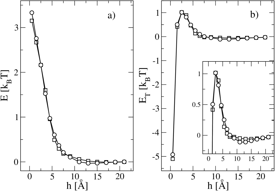
Figure 5: a) Potential of mean force, $E(h)$, as obtained by integration of the total force as a function of $h$. b) The same data plus the macroparticle-macroparticle Hamaker contribution of polystyrene in water, $E_{T}(h)$. The inset zooms in the data of panel b).

Forces are easily translated into potentials of mean force by means of

$$E(h)=\int_{\infty}^{h}F_{t}(x)dx.$$ (9)

$E(h)$ is plotted in Fig. 5 a) as a function of the separation distance $h$ for both systems. As mentioned, $E(h)$ is similar for the cationic and anionic systems for all $h$. In Fig. 5 b) it is plotted the same data plus the Hamaker contribution, $E_{T}(h)=E(h)+E_{H}(h)$, which reads Hunter

$$\!E_{H}(h)\!=\!\frac{-A_{H}}{6}\!\!\left[\!\frac{2a_{M}^{2}}{h(4a_{M}\!+\!h)}\!+\!\frac{2a_{M}^{2}}{(2a_{M}\!+\!h)^{2}}\!+\!\ln\!\left(\!\frac{h(4a_{M}\!+\!h)}{(2a_{M}\!+\!h)^{2}}\!\right)\right]$$ (10)

being $A_{H}=0.95\times 10^{-20}$J the Hamaker constant for polystyrene in water and $a_{M}=25\mbox{\AA}$ the colloidal particle (macroparticle) radius. Panel b) of Fig. 5 shows the existence of a potential barrier peaking at $h=2.5\mbox{\AA}$ even for a 0.6 M electrolyte concentration. This contrasts the DLVO theory predictions (no barrier for this salt concentration). As was pointed out, the potential barrier is related to the accumulation of counterions around the surface-surface contact region. That is, work must be done by or on the system in order to release the counterions from the very low energy region in-between the particles surfaces to relocate them in a less favorable place. According to the simulation data this work is not compensated by the gain of the Hamaker contribution. This result agrees with the experimental values found for the probability of forming a primary bond, $P_{1}$, which are for all cases smaller than one. If this were true, the dimmer formation rate constant $k_{11}$ would approach better the theoretical Smoluchowsky value, $k^{Smol}_{11}=11.1\times 10^{-18}$ m³/s (water at 293 K), and the overall effect of hydrodynamic interactions would be less important than generally accepted (hydrodynamic interactions are said to decrease the Smoluchowsky value in a factor of two spielman70 ; honig71 ).

It should also be noted that the secondary minima shown in Fig. 5 b) are not deep enough to produce relatively stable secondary bonds. This is expected for small particles as the ones considered for the simulations. For much larger particles, as these employed to obtain the experimental data shown in Fig. 1, the Hamaker contribution enlarges producing the well known secondary minimum. Additionally, according to the fitted $\tau_{2}$ parameter, the secondary minimum for the cationic case should be deeper than the one corresponding to the anionic particles. This is not captured by the simulations. Finally, the obtained primary minima are too deep to allow for bond breakup. Note that equation 10 diverges for $h\rightarrow 0$ and thus it surely overestimates the real Hamaker contribution for very short distances (first point of panel b) of Fig. 5 is evaluated at $h=0.1\mbox{\AA}$). Additionally, other contributions are expected to be relevant at these very short distances (for instance, water molecules hydrating surface charges must also be released from the in-between region to produce a bare-bare bond).

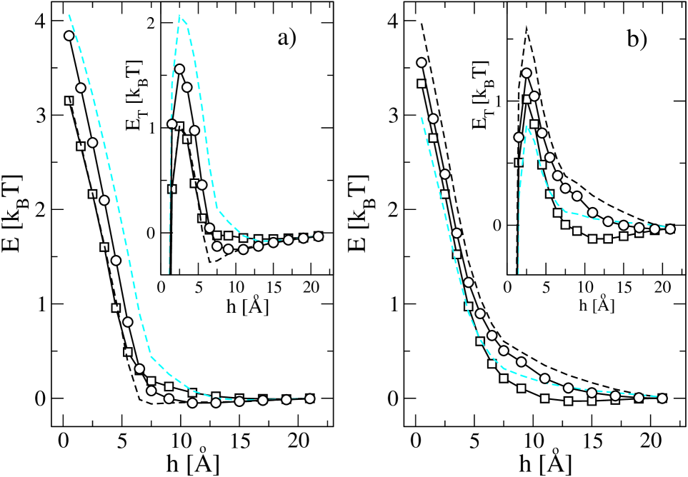
Figure 6: Potential of mean force, $E(h)$, as a function of the separation distance, $h$, for a) the cationic system, and b) the anionic system. The insets show the same data plus the Hamaker contribution, $E_{T}(h)$. Squares correspond to NaCl, whereas circles correspond to NaSCN with $a_{a}=2.75\mbox{\AA}$. Dark dashed and light dashed lines correspond to NaSCN with $a_{a}=2.50\mbox{\AA}$ and $3.00\mbox{\AA}$, respectively.

Up to this point the calculations only considered NaCl as the dissolved salt. From here on we focus on the results for NaSCN for different SCN^- hydrated radius, $a_{a}$, keeping constant the fitted Na⁺ radius (NO${}_{3}^{-}$ is expected to show an intermediate behavior between Cl^- and SCN^- and so, it is not considered for the simulations). As mentioned at the end of section II, the parameters obtained from the fitting procedure to the aggregation data suggest the following changes of $E_{T}(h)$ when comparing the NaCl with the NaSCN cases: i) An increase of the $E_{T}(h)$ peak for both, the cationic and the anionic system, in correspondence with the $P_{1}$ decrease when aggregation is induced by NaSCN. This increase should be similar for both systems ($P_{1}$ decreases similarly in both systems). ii) An increase of the potential contact value, $E_{T}(h=0)$, for the cationic system, and a similar value of $E_{T}(h=0)$ for the anionic system. This is in correspondence with the obtained decrease of $\tau_{1}$ for the cationic system and the constant value of $\tau_{1}$ for the anionic colloidal particles. iii) Next, the smaller values of $\tau_{2}$ found for NaSCN would translate in a decrease of the depth of the secondary minimum for NaSCN. This would also apply for both latices. In addition, the depth of the secondary minima for all electrolytes and for the anionic case should be smaller than those corresponding to the cationic case. iv) Finally, the simulations should also produce a greater adsorption of the SCN^- ion for both systems. This is to agree with the increase of the mobility values obtained for the anionic system when changing from NaCl to NaSCN electrolyte, as well as with the mobility reversal of the cationic particles (see the mobility data included in Table 1).

The results of the calculations involving the NaSCN are given in Fig. 6. For an easy comparison, the data obtained for the NaCl are also included as squares. Fig. 6 a) corresponds to the cationic system and Fig. 6 b) to the anionic one. The insets show the same energy data plus the Hamaker contribution. From Fig. 6 a) it is seen that the anionic radius, $a_{a}$, must be larger than $2.5\mbox{\AA}$ to obtain a higher repulsive barrier and a higher $E_{T}(h=0)$ for NaSCN than for NaCl. This is so since the PMF of the positive colloidal particles increases with the anion size. On the contrary, Fig. 6 b) shows that the PMF of the anionic system decreases with the SCN^- size, producing a smaller energetic barrier than the NaCl reference for $a_{a}<2.5\mbox{\AA}$. Thus, according to the model, SCN^- should have a hydrated size ranging in [2.5; 3.0]Å to match the $P_{1}$ decrease found for both latices from the master equation fits. This is a reasonable range for the hydrated size of SCN^-. Fig. 6 includes the calculations for $a_{a}=2.75\mbox{\AA}$ (open circles). For this anionic size both panels of Fig. 6 show energetic barriers larger than those obtained with NaCl (insets of Fig. 6), in agreement with point i) of previous paragraph. Additionally, for the cationic system (panel a)) $E_{T}(h=0)$ is clearly larger for SCN^- than for Cl^-, whereas the increase is less pronounced for the anionic system (panel b)). So, point ii) of previous paragraph is qualitatively matched. Point iii) is partially matched. That is, for the cationic system, the depth of the secondary minima decreases only for NaSCN with $a_{a}=3.00\mbox{\AA}$, but not for $a_{a}=2.75\mbox{\AA}$ as it should. On the other hand, the secondary minima for the cationic system are deeper than for the anionic system for NaSCN, which is right. In fact, the secondary minimum disappears for the anionic system and the broadness of the energetic barrier turns significantly larger. This longer range of the PMF barrier suggests that pairs of counter and coions must be released from the in-between surface-surface region to produce a stable bond. Summarizing, in general and up to this point, the qualitative agreement between the suggested trends from the fitted parameters and the simulation results is good. This enhances confidence in both treatments.

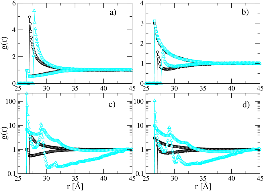
Figure 7: Radial distribution functions, $g(r)$, for Na⁺ (squares), Cl^- (circles), and SCN^- ions (triangles), with respect to an isolated positive a) and negative b) macroparticle. Black lines and symbols correspond to NaCl runs and light (cyan) lines and symbols correspond to NaSCN runs with $a_{a}=2.75\mbox{\AA}$. Panels c) and d) show the data corresponding to a SCN^- hydrated radius of $a_{a}=1.5\mbox{\AA}$. As reference, these panels also include the NaCl data shown in panels a) and b).

Unfortunately, point iv) is not fulfilled. The radial distribution functions obtained for an isolated colloidal particle immersed in NaCl electrolyte solution and in a NaSCN electrolyte solution (with $a_{a}=2.75\mbox{\AA}$) show no practical differences for the adsorption of SCN^- and Cl^-. This is shown in panels a) and b) of Fig. 7 for the positive and negative systems, respectively. This suggests that some SCN^- anions should be partially losing their water shells in order to attach the colloidal particles surfaces. To confirm this solvent mediated mechanism simulations explicitly accounting for the solvent molecules are needed (recently, potentials of mean force were build up directly from force fields Kalcher10 ; Fyta10 ). Nonetheless, with the employed model we can explore the effect of the SCN^- hydrated size on their adsorption on the colloidal particles surfaces. For this purpose an extra calculation is made for an isolated colloidal particle immersed in SCN^- with $a_{a}=1.5\mbox{\AA}$. This would represent the size of a partially hydrated SCN^- ion. Results are shown in panels c) and d) of Fig. 7. These panels show a very large adsorption of SCN^- for both cases (positive, a), and negative, b), colloidal particles). Furthermore, both, counterions and coions radial distribution profiles show several peaks which reveals the appearance of charge reversal Felipe08 ; Martin-Molina09a (for the positive chase) and overcharging Mesina09 ; Boinovich10 (for the negative case) phenomena. Indeed, the contact peak of the radial distribution function for the positive system is produced by the adsorption of approximately 90 anions. For the anionic system, the number of absorbed SCN^- ions average 55. This leads to an effective surface charge density at $3\mbox{\AA}$ from the surface close to -100 mC/m² (accounting for both, the adsorbed anions and cations) for the cationic system and -108 mC/m² for the anionic one. That is, the effective surface charge density of the anionic system double (overcharging), and the cationic system not only change sign (charge reversal), but also double its original absolute value. Thus, the adsorption is strongly overestimated by these calculations which signal the extreme sensitivity to the considered hydrated radius of the ions Martin-Molina09a ; Martin-Molina09b ; Quesada-Perez10 (sensitivity to this parameter is strongly enhanced when including the dispersion contribution). However, since the dehydrating process is energetically demanding, not all the SCN^- ions placed close to the colloidal particle surface are expected to follow this rout. Consequently, a significant but not very large amount of ions should dehydrate while adsorbing, explaining the mobility measurements, whereas at larger separations from the colloidal particles surfaces, anions would be fully hydrated to produce forces such as those obtained for a SCN^- radius of $2.75\mbox{\AA}$. These adsorbed and partially dehydrated ions should also increase the potential energy at very short distances, which aids explaining the full reversibility of the primary bonds for the cationic system. Probably these ions are not being totally removed from the surfaces while forming a primary bond leading to their occlusion. This phenomenon was recently proposed (for hydronium ions) to explain the observed reduction of surface charges during the aggregation and coalescence of elastomer particles Gauer10 .

V Conclusions

Population balance fitting of experimental aggregation data and potentials of mean force from simulations support the existence of an energetic barrier for the potential of mean force between hydrophobic colloidal particles at high electrolyte concentrations. This is found not only for NaSCN but even for NaCl, although the barrier is smaller in this last case. Furthermore, positive and negative colloids show the same increasing trend for the height of the energetic barrier following the series NaCl, NaNO₃, NaSCN. These findings contrast the DLVO predictions. For positive particles, the energetic barrier would be produced by the work needed for releasing the adsorbed counterions from the in-between surface-surface region and relocating them in a not so energetically favorable place. Thus, the barrier would be located at very short surface-surface distances. In the case of negative colloids, the barrier extends to larger distances suggesting that pairs of counter and coions must be released from the in-between surface-surface region to produce a stable bond. According to simulations and population balance fitting, ions like SCN^-, which show a natural tendency to adsorb onto hydrophobic surfaces, produce a larger energetic barrier for positive and negative surfaces. In the case of the positive colloidal particles, SCN^- produces weaker primary bonds yielding a clear reversibility of the aggregation processes.

VI Acknowledgements

The author thanks fruitful and enrichment discussions with Drs. Teresa López-León, Juan Manuel López-López, Delfi Bastos-González, Juan Luis Ortega-Vinuesa, and Manuel Quesada-Perez.

References

- (1) R. J. Hunter, Foundations of Colloid Science, 2nd ed. (Oxford University Press, New York, 2001).
- (2) K. D. Collins and M. W. Washabaugh, Q. Rev. Biophys. 18, 323 (1985).
- (3) M. G. Cacace, E. M. Landau, and J. J. Ramsden, Q. Rev. Biophys. 30, 241 (1997).
- (4) L. Boinovich, Curr. Opin. Colloid Interface Sci. 15, 297 (2010).
- (5) F. Tavares, D. Bratko, H. W. Blanch, and J. M. Prausnitz, J. Phys. Chem. B 108, 9228 (2004).
- (6) M. Manciu and E. Ruckenstein, Langmuir 21, 11312 (2005).
- (7) M. Boström, W. Kunz, and B. Ninham, Langmuir 21, 2619 (2005).
- (8) M. Quesada-Perez, R. Hidalgo-Alvarez, and A. Martin-Molina, Colloid Polym. Sci. 288, 151 (2010).
- (9) I. Kalcher, J. Schulz, and J. Dzubiella, J. Chem. Phys. 133, 164511 (2010).
- (10) T. Lopez-Leon, J. Lopez-Lopez, G. Odriozola, D. Bastos-Gonzalez, and J. Ortega-Vinuesa, Soft Matter 6, 1114 (2010).
- (11) D. T. Gillespie, J. Phys. Chem. 81, 2340 (1977).
- (12) M. Thorn and M. Seesselberg, Phys. Rev. Lett. 72, 3622 (1994).
- (13) M. Thorn, M. L. Broide, and M. Seesselberg, Phys. Rev. E. 51, 4089 (1995).
- (14) I. M. Elminyawi, S. Gangopadhyay, and C. M. Sorensen, J. Colloid Interface Sci. 144, 315 (1991).
- (15) E. Pefferkorn and J. Widmaier, Colloids Surf. 145, 25 (1998).
- (16) X. Feng and L. Xiao-Yan, Water Sci. Technol. 57, 151 (2008).
- (17) M. von Smoluchowski, Phys. Z. 17, 557 (1916).
- (18) M. von Smoluchowski, Z. Phys. Chem. 92, 129 (1917).
- (19) G. Odriozola, A. Schmitt, J. Callejas-Fernández, R. Martínez-García, R. Leone, and R. Hidalgo-Álvarez, J. Phys. Chem. B 107, 2180 (2003).
- (20) G. Odriozola, A. Schmitt, Moncho-Jordá, J. Callejas-Fernández, R. Martínez-García, R. Leone, and R. Hidalgo-Álvarez, Phys. Rev. E. 65, 031405 (2002).
- (21) G. Odriozola, A. Moncho-Jordá, A. Schmitt, J. Callejas-Fernández, R. Martínez-García, and R. Hidalgo-Álvarez, Europhys. Lett. 53, 797 (2001).
- (22) M. Lattuada, P. Sandkuhler, H. Wu, J. Sefcik, and M. Morbidelli, Adv. Colloid Interface Sci. 103, 33 (2003).
- (23) M. Lattuada, H. Wu, P. Sandkuhler, J. Sefcik, and M. Morbidelli, Chem. Eng. Sci. 59, 1783 (2004).
- (24) M. Lattuada, H. Wu, J. Sefcik, and M. Morbidelli, J. Phys. Chem. B 110, 6574 (2006).
- (25) G. Odriozola, R. Leone, A. Schmitt, J. Callejas-Fernández, R. Martínez-García, and R. Hidalgo-Álvarez, J. Chem. Phys. 121, 5468 (2004).
- (26) H. Sonntag and K. Strenge, Coagulation Kinetics and Structure Formation (Plenum Press, New York, 1987).
- (27) P. Meakin, Fractals, scaling and growth far from equilibrium (Springer, Cambridge, 1998).
- (28) M. Y. Lin, H. M. Lindsay, D. A. Weitz, R. Klein, R. C. Ball, and P. Meakin, Phys. Condens. Matter 2, 3093 (1990).
- (29) M. Y. Lin, H. M. Lindsay, D. A. Weitz, R. C. Ball, R. Klein, and P. Meakin, Phys. Rev. A 41, 2005 (1990).
- (30) M. Tirado-Miranda, A. Schmitt, J. Callejas-Fernandez, and A. Fernandez-Barbero, Langmuir 15, 3437 (1999).
- (31) S. Babu, J. Gimel, and T. Nicolai, Eur. Phys. J. E 27, 297 (2008).
- (32) S. Babu, J. Gimel, and T. Nicolai, J. Chem. Phys. 125, 184512 (2006).
- (33) S. Babu, J. Gimel, and T. Nicolai, J. Chem. Phys. 127, 054503 (2007).
- (34) N. Kovalchuk, V. Starov, P. Langston, and N. Hilal, Colloid J. 71, 503 (2009).
- (35) N. Kovalchuk, V. Starov, P. Langston, and N. Hilal, Adv. Colloid Interface Sci. 147, 144 (2009).
- (36) G. Odriozola, R. Leone, A. Moncho-Jorda, A. Schmitt, and R. Hidalgo-Alvarez, Physica A 335, 35 (2004).
- (37) H. Wu, M. Lattuada, P. Sandkuhler, J. Sefcik, and M. Morbidelli, Langmuir 19, 10710 (2003).
- (38) A. E. Gonzalez, Phys. Rev. E. 74, 061403 (2006).
- (39) A. E. Gonzalez, Europhys. Lett. 73, 878 (2006).
- (40) F. Jiménez-Ángeles, G. Odriozola, and M. Lozada-Cassou, J. Chem. Phys. 124, 134902 (2006).
- (41) G. Odriozola, F. Jiménez-Ángeles, and M. Lozada-Cassou, Phys. Rev. Lett. 97, 018102 (2006).
- (42) M. Boström, F. Tavares, B. Ninham, and J. M. Prausnitz, J. Phys. Chem. B 110, 24757 (2006).
- (43) E. Lima, F. Tavares, and E. Biscaia, Phys. Chem. Chem. Phys. 9, 3174 (2007).
- (44) Z. Jin and J. Wu, J. Phys. Chem. B 115, 1450 (2011).
- (45) L. A. Spielman, J. Colloid Interface Sci. 33, 562 (1970).
- (46) E. P. Honig, G. J. Roebersen, and P. H. Wiersema, J. Colloid Interface Sci. 36, 97 (1971).
- (47) M. Fyta, I. Kalcher, J. Dzubiella, L. Vrbka, and R. Netz, J. Chem. Phys. 132, 024911 (2010).
- (48) F. Jiménez-Ángeles and M. Lozada-Cassou, J. Chem. Phys. 128, 174701 (2008).
- (49) A. Martin-Molina, R. Hidalgo-Alvarez, and M. Quesada-Perez, J. Phys.: Condens. Matter 21, 424105 (2009).
- (50) R. Mesina, J. Phys.: Condens. Matter 21, 113102 (2005).
- (51) A. Martin-Molina, J. G. Ibarra-Armenta, and M. Quesada-Perez, J. Phys. Chem. B 113, 2414 (2009).
- (52) C. Gauer, H. Wu, and M. Morbidelli, J. Phys. Chem. B 114, 8838 (2010).